Spatial Stimuli Gradient Sketch Model

Abstract

The inability of automated edge detection methods inspired from primal sketch models to accurately calculate object edges under the influence of pixel noise is an open problem. Extending the principles of image perception i.e. Weber- Fechner law, and Sheperd similarity law, we propose a new edge detection method and formulation that use perceived brightness and neighbourhood similarity calculations in the determination of robust object edges. The robustness of the detected edges is benchmark against Sobel, SIS, Kirsch, and Prewitt edge detection methods in an example face recognition problem showing statistically significant improvement in recognition accuracy and pixel noise tolerance.

I Introduction

The concept of spatial change detection is interrelated to the primal sketch theory [1, 2, 3] where the change in the intensities over a visual field is taken as feature than pixel intensities themselves. The primal sketch relates the geometry of the image intensity changes in the images to the early psychophysical mechanism of human eye. These edge models reflect to the general idea of spatial change detection [4] from the neighbourhood of the pixel under consideration that find application as a feature preprocessing stage in general image bases pattern recognition problems [5, 6].

This paper presents a noise robust edge detection method using the local stimuli computed from the amount perceived brightness at each image location for enhancing the quality of image inherent structural and intensity edge information. The proposed method computes a relative numerical quantification of the physical stimuli contributed to the image formation. Such computed local stimuli helps to extract and preserve underlying structural edge details. The quality of the detected edges are demonstrated through examples of simulations with hypothetical edges and through standard face recognition problem.

II Background

In digital images, object details are analyzed with the help of responses computed for intensity changes at its boundaries that are referred to as the edges [7]. This primary idea is inspired by the biological vision processing of human eye and in its early form is formulated by primal sketch model [2] describes an image using the image inherent structures based on the response computed with respect to edge formations using optimal smoothing filters and detection of intensity changes.

The primary criteria of any edge detection technique include its ability to provide best response to edges, good localization, continuity of edges and tolerance to image noise cum natural variance within the same regions. A comprehensive description of an image inevitably requires a robust retrieval of edge information by satisfying the criteria for edge detection. The quality of image description based on primal sketch model can be mathematically modeled with help of sketchable and unsketchable edge responses [2]. The term sketchability is meant for useable edges and unsketchable edge responses are referred to the false edges formed due the intra-region variability together with the image noise. Primal structures retrieved comprising of all sketchable edges can be described as the ideal edge detection technique. In real world images, it is not possible to perform an ideal detection, but to optimize for minimal trade-off between sketchable and unsketchable edges the best efforts are made by applying smoothing as the first stage of edge detection. Unfortunately, this will contribute to reduction of many of the fine details due to the averaging operations used to implement the smoothing. This effect can be controlled up to certain degrees, by using specialized structure preserved denoising techniques such as non-local means filter [8], noise suppression filters [9, 10], and anisotropic diffusion filtering [11]. On the other hand, hypothetically, an edge response computation with inherent intra-region variability suppression can lead to more robust edge detection approaches. In this paper, the focus is on the suppression of intensity variability other than edges in order to minimizes the unsketchable primitives.

III Proposed Method

We propose to make use of Weber-Fechner’ law [12] to mathematically compute the amount of perceived brightness and the corresponding local stimuli. The aim is to enhance the inherent image features by weighting the original image using the magnitude of local stimuli resulting in the image formation. This magnitude of local stimuli is computed by finding the local variation in perceived brightness at the respective locations. Fechner law states that the amount of perceived brightness/loudness is equal to the logarithm the measured intensity of the physical stimulus. Thus, the perceived brightness, $B_{p}$ for a given image $I$, is expressed as

$$B_{p}=k\log_{10}(I)$$ (1)

where $k$ is a constant.

The gradients of the perceived brightness would represent the edge information in the image. Since the gradient itself is a linear operator the noisy pixel will not be suppressed by this operation. In addition, the gradient is a form of distance measure in context of measuring the localised inter-pixel variability. While there exists several of distance measures that are suitable to be used for detecting the spatial change [4], we propose to use Shepherd’s similarity measure [13] that would give a measure of perceived similarity on the measured distance. In addition to the psychological dimension of the Shepherd’s similarity, this measure has the ability to suppress the outliers in the distance calculations due to the exponential nature of the transform. Applying this theory to practise, localized spatial stimuli magnitude is numerically quantified as the net variation of perceived brightness along $x$ and $y$ directions. The variation of $B$ along $x$ ($V_{x}$) and $y$ ($V_{y}$) directions is computed as a function of respective gradients ($g_{x}$ and $g_{y}$) and is expressed as:

$$V_{x}=g_{x}.\exp(-|g_{x}|)~{};~{}V_{y}=g_{y}.\exp(-|g_{y}|)$$ (2)

The magnitude of local stimuli ($V$) can be computed using Eq. 3.

$$V=\sqrt{V_{x}^{2}+V_{y}^{2}}$$ (3)

The inherent image features by pixel wise weighting of original image (Fig. 1a) is computed using Eq. 3 to obtain the local stimuli magnitude map ($V$) (Fig. 1b).

Figure 1: (a) Original image $I$, (b) Local stimuli magnitude map $V$

Algorithm 1 Local Stimuli Template

1:procedure LST($I$)

2:     Read image, $I$.

3:     $B\leftarrow k\log(I)$ // Perceived brightness

4:     $[g_{x},g_{y}]\leftarrow gradient(B)$. // Gradient operation, using central differencing scheme.

5:     $V_{x}\leftarrow g_{x}\exp(-|g_{x}|)$ // Local change in brightness (stimuli) along x axis.

6:     $V_{y}\leftarrow g_{y}\exp(-|g_{y}|)$ //Local change in brightness (stimuli) along y axis.

7:     $V\leftarrow\sqrt{V_{x}^{2}+V_{y}^{2}}$ //Local stimuli map.

8:end procedure

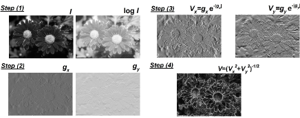
Algorithm 1 provides the formal summary of the proposed feature enhancement process based on local stimuli weighting. Figure 2 shows a step wise graphical illustration of algorithm 1 and indicates the proposed methods ability to detect and amplify edge signals in step 3-4. The proposed method retrieve edges by computing the local stimuli experienced at each pixel location with the help of the amount of brightness perceived to form the image. The local stimuli is computed as the two dimensional variations in perceived brightness. The natural variability in computed brightness is observed to be less; at the same time edge information is sufficient to compute the responses. Also exponential weights are introduced to the filtering scheme, which further helps in the suppression of intra-region intensity variability.

Figure 2: A graphical illustration on the working of the proposed edge detection method.  

Figure 3 illustrates the comparison of the proposed method for the amount of underlying structural information extracted with that of the existing methods such as Sobel, SIS, Kirsch, and Prewitt [14] for a sample face image. The images visually illustrate that the proposed method produces meaningful edge features compared to other methods, where the binary edges are obtained using the adaptive Ostu’s threshold technique[15]. Proposed method shows least spurious structures with much better distinction from corresponding background. Edge responses computed for a set of images with diverse imaging conditions from Berkeley Segmentation Dataset is displayed in Fig. 4.

(a) Sobel

(b) SIS

(c) Kirsch

(d) Prewitt

(e) Proposed

(f) Sobel

(g) SIS

(h) Kirsch

(i) Prewitt

(j) Proposed

Figure 3: Detected edges and binary maps computed for visualizing edge response (a-e) and the underlying structural details (f-j) of original image extracted using various methods namely Sobel, SIS, Kirsch and Prewitt, in comparison to the proposed method

Figure 4: Edge responses computed for natural scenes shared by Berkeley Segmentation Dataset, with original images (a-e) and corresponding edge responses (f-j).

IV Experimental Results

For better understanding, the responses to edge computed for classical primal sketch model and proposed scheme for various shapes are shown in Table I,II,III. Table I illustrates the edges computed for varying gaussian noise ($\sigma_{nv}^{2}$) in the order of 0%, 5%, 10%, and 20% of the maximum of image intensities for step-edge. From results, primal sketch model based scheme fails to detect edges beyond 5% increase in variability, whereas the proposed method is proves to be capable of detecting edges even at 20% intensity variability. This indicates the proposed method”s capability in extracting maximum number of sketchable edges with minimal unsketchable details.

Table II illustrates the response on Gaussian shaped intensity changes with increasing intensity variability. Results depicts that the primal sketch model without smoothing fails even with slight increase in variability. Whereas, the proposed method shows a good tolerance against increasing intensity variability with a comparable edge localization. Table III depicts spatial edge response for a ramp shape, where it can be observed that variability tolerance for method schemes are very poor, whereas the proposed method is shown to be more robust to pixel noise.

TABLE I: Comparison of Edge Responses computed using a step shape for varying percentile standard deviations in reference to the maximum intensity value

$\sigma_{nv}^{2}$(%)	Original	Primal Sketch Model	Proposed
0
5
10
20

TABLE II: Comparison of Edge Responses computed using a Gaussian shape for varying percentile standard deviations in reference to the maximum intensity value

$\sigma_{nv}^{2}$(%)	Original	Primal Sketch Model	Proposed
0
5
10
20

TABLE III: Comparison of Edge Responses computed using a ramp shape for varying percentile standard deviations in reference to the maximum intensity value

$\sigma_{nv}^{2}$(%)	Original	Primal Sketch Model	Proposed
0
5
10
20

Face images are used to study the quality of the edges detected by our proposed method in a realistic imaging condition. Performance evaluation of the proposed method is quantified using percentage correctness, with the test data sets selected from face databases namely, ORL, AR, GeorgiaTech (GTech), and Japanese Female Facial Expression (JAFFE), These databases cover a wide range of imaging conditions. Unless otherwise specified, the proposed method is evaluated against other commonly used edge detection methods such as Prewitt, Kirsch, SIS and Sobel using a minimum distance nearest neighbour classifier.

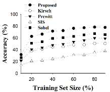
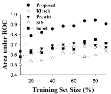
The recognition accuracy and area under receiver operator characteristics curve, for varying size of the training set is illustrated with the help of Fig. 5 using average performances from databases ORL, AR, GTech, and JAFFE. In a general, the proposed method shows a consistent improvement in robustness over the other methods.

Figure 5: Average variation in accuracy (%) (a), and area under ROC (b) for varying sizes of training set (%) computed for ORL, AR, Georgia Tech, and JAFFE face databases calculated using a lazy classifier.

The comparisons of average recognition accuracy on different classifiers are tabulated for proposed method benchmark against Kirsch, Prewitt, SIS, and Sobel edge detection methods in Tables IV using databases ORL, AR, GTech, and JAFFE. The classification experiments are conducted by dividing the database into equal sized sets of training and test images. The classifiers used in the recognition experiments are IB-k[16], NNge[17], random forest[18], and SMO[19]. The results indicate statistically significant improvement in robustness of the proposed edge features over the existing edge models.

TABLE IV: Average recognition accuracy (%) for different classifiers using face databases ORL, AR, Georgia Tech, and JAFFE

Method	Database
	IBk	NNge	RandomForest	SMO
Proposed	76.1$\pm$6.4	67.0$\pm$9.2	41.4$\pm$9.3	80.9$\pm$6.1
Kirsch	46.8$\pm$8.5	41.6$\pm$9.7	32.2$\pm$8.4	62.02$\pm$8.9
Prewitt	54.3$\pm$8.2	44.9$\pm$7.8	34.4$\pm$7.2	61.6$\pm$8.1
SIS	31.2$\pm$8.2	25.6$\pm$7.2	20.1$\pm$8.9	39.5$\pm$8.8
Sobel	63.6$\pm$7.5	50.1$\pm$11.1	40.7$\pm$10.5	77.1$\pm$8.5

Figure 6: Average accuracy computed from example AR face database illustrating the impact of percentage intensity variability in pixels. Here, x axis represents the maximum additive noise variance per pixel.

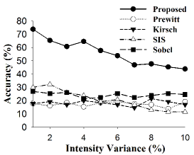
The proposed edge model contribute to reducing intra-regional intensity variance that in turn reflects improvements in the recognition accuracy. For illustrating the effect, face databases are added with additive noise variance in increasing order. Figure 6 show significantly better tolerance towards intensity variance in comparison to other methods. The proposed theory preserves the edge information using fundamental principles from the psychology of vision processing. While the noise itself is not substantially removed as seen from Table I, II, III, and Fig 5, 6, while it does indicate that edges are preserved and that it can be processed further using filtering schemes to retrieve edges close to its non-noisy state.

V Conclusion

In this paper, we presented the idea of spatial stimuli gradient sketch model inspired from the Fechner and Weber law, and Sheperd similarity measure that enables relationships between the image intensity and psychological measurement space. The use of these concepts results in edges that are robust to noise in pixels intensity along the edges of different nature and overcome the limitations of edges based on primal sketch models. The robustness of the method is illustrated with the help of face recognition experiments on some of the standard benchmark databases that cover the wide range of possible edges in the digital images. The use of proposed method showed a statistically significant improvement in the recognition accuracies over the benchmark edge detection methods. The comparison shown in Fig 6 indicate that while almost every benchmark edge detection methods fail to work as useful features in a face recognition problem, the proposed edges show a higher level of tolerance to pixel noise levels. In future, the proposed spatial stimuli gradient sketch model can be used to extract more useful features for a wide range of problems such as image registration, image recognition, and image segmentation, where the use of edges is proven to be useful and higher levels of abstraction shown to improve the performances.

References

- [1] C.-e. Guo, S. C. Zhu, and Y. N. Wu, “Towards a mathematical theory of primal sketch and sketchability,” in Computer Vision, 2003. Proceedings. Ninth IEEE International Conference on. IEEE, 2003, pp. 1228–1235.
- [2] D. Marr and E. Hildreth, “Theory of edge detection,” Proceedings of the Royal Society of London. Series B. Biological Sciences, vol. 207, no. 1167, pp. 187–217, 1980.
- [3] E. C. Hildreth, “Implementation of a theory of edge detection,” AI Technical Reports, MIT, 1980.
- [4] A. P. James and S. Dimitrijev, “Face recognition using local binary decisions,” Signal Processing Letters, IEEE, vol. 15, pp. 821–824, 2008.
- [5] N. McLaughlin, J. Ming, and D. Crookes, “Robust multimodal person identification with limited training data,” Human-Machine Systems, IEEE Transactions on, vol. 43, no. 2, pp. 214–224, 2013.
- [6] A. Pappachen James and S. Dimitrijev, “Inter-image outliers and their application to image classification,” Pattern recognition, vol. 43, no. 12, pp. 4101–4112, 2010.
- [7] L. S. Davis, “A survey of edge detection techniques,” Computer graphics and image processing, vol. 4, no. 3, pp. 248–270, 1975.
- [8] A. Buades, B. Coll, and J.-M. Morel, “A non-local algorithm for image denoising,” in Computer Vision and Pattern Recognition, 2005. CVPR 2005. IEEE Computer Society Conference on, vol. 2. IEEE, 2005, pp. 60–65.
- [9] D. H. Lim, “Robust edge detection in noisy images,” Computational Statistics & Data Analysis, vol. 50, no. 3, pp. 803–812, 2006.
- [10] G. Sun, Q. Liu, Q. Liu, C. Ji, and X. Li, “A novel approach for edge detection based on the theory of universal gravity,” Pattern Recognition, vol. 40, no. 10, pp. 2766–2775, 2007.
- [11] P. Perona and J. Malik, “Scale-space and edge detection using anisotropic diffusion,” Pattern Analysis and Machine Intelligence, IEEE Transactions on, vol. 12, no. 7, pp. 629–639, 1990.
- [12] S. Hecht, “The visual discrimination of intensity and the weber-fechner law,” The Journal of general physiology, vol. 7, no. 2, pp. 235–267, 1924.
- [13] R. N. Shepard, “Toward a universal law of generalization for psychological science,” Science, vol. 237, no. 4820, pp. 1317–1323, 1987.
- [14] M. Kunt, “Edge detection: A tuttorial review,” in Acoustics, Speech, and Signal Processing, IEEE International Conference on ICASSP’82., vol. 7. IEEE, 1982, pp. 1172–1175.
- [15] N. Otsu, “A threshold selection method from gray-level histograms,” Automatica, vol. 11, no. 285-296, pp. 23–27, 1975.
- [16] D. Aha and D. Kibler, “Instance-based learning algorithms,” Machine Learning, vol. 6, pp. 37–66, 1991.
- [17] B. Martin, “Instance-based learning: Nearest neighbor with generalization,” Master’s thesis, University of Waikato, Hamilton, New Zealand, 1995.
- [18] L. Breiman, “Random forests,” Machine Learning, vol. 45, no. 1, pp. 5–32, 2001.
- [19] T. Hastie and R. Tibshirani, “Classification by pairwise coupling,” in Advances in Neural Information Processing Systems, M. I. Jordan, M. J. Kearns, and S. A. Solla, Eds., vol. 10. MIT Press, 1998.