A Row-parallel 8$\times$8 2-D DCT Architecture Using Algebraic Integer Based Exact Computation

Abstract

An algebraic integer (AI) based time-multiplexed row-parallel architecture and two final-reconstruction step (FRS) algorithms are proposed for the implementation of bivariate AI-encoded 2-D discrete cosine transform (DCT). The architecture directly realizes an error-free 2-D DCT without using FRSs between row-column transforms, leading to an 8$\times$8 2-D DCT which is entirely free of quantization errors in AI basis. As a result, the user-selectable accuracy for each of the coefficients in the FRS facilitates each of the 64 coefficients to have its precision set independently of others, avoiding the leakage of quantization noise between channels as is the case for published DCT designs. The proposed FRS uses two approaches based on (i) optimized Dempster-Macleod multipliers and (ii) expansion factor scaling. This architecture enables low-noise high-dynamic range applications in digital video processing that requires full control of the finite-precision computation of the 2-D DCT. The proposed architectures and FRS techniques are experimentally verified and validated using hardware implementations that are physically realized and verified on FPGA chip. Six designs, for 4- and 8-bit input word sizes, using the two proposed FRS schemes, have been designed, simulated, physically implemented and measured. The maximum clock rate and block-rate achieved among 8-bit input designs are 307.787 MHz and 38.47 MHz, respectively, implying a pixel rate of 8$\times$307.787$\approx$2.462 GHz if eventually embedded in a real-time video-processing system. The equivalent frame rate is about 1187.35 Hz for the image size of 1920$\times$1080. All implementations are functional on a Xilinx Virtex-6 XC6VLX240T FPGA device.

Keywords
DCT, Algebraic Integer Quantization, FPGA design

1 Introduction

High-quality digital video in multimedia devices and video-over-IP networks connected to the Internet are under exponential growth and therefore the demand for applications capable of high dynamic range (HDR) video is accordingly increasing. Some HDR imaging applications include automatic surveillance [1, 2, 3, 4], geospatial remote sensing [5], traffic cameras [6], homeland security [4], satellite based imaging [7, 8, 9], unmanned aerial vehicles [10, 11, 12], automotive industry [13], and multimedia wireless sensor networks [14]. Such HDR video systems operating at high resolutions require an associate hardware capable of significant throughput at allowable area-power complexity.

Efficient codec circuits capable of both high-speeds of operation and high numerical accuracy are needed for next-generation systems. Such systems may process massive amounts of video feeds, each at high resolution, with minimal noise and distortion while consuming as little energy as possible [15].

The two-dimensional (2-D) discrete cosine transform (DCT) operation is fundamental to almost all real-time video compression systems. The circuit realization of the DCT directly relates to noise, distortion, circuit area, and power consumption of the related video devices [15]. Usually, the 2-D DCT is computed by successive calls of the one-dimensional (1-D) DCT applied to the columns of an 8$\times$8 sub-image; then to the rows of the transposed resulting intermediate calculation [16]. The VLSI implementation of trigonometric transforms such as DCT and DFT is indeed an active research area [17, 18, 19, 20, 21, 22, 23, 24, 25, 26, 27, 28, 29, 30, 31, 32, 33].

An ideal 8-point 1-D DCT requires multiplications by numbers in the form $c[n]=\cos(n\pi/16)$, $n=0,1,\ldots,7$. These constants impose computational difficulties in terms of number binary representation since they are not rational. Usual DCT implementations adopt a compromise solution to this problem employing truncation or rounding off [34, 35] to approximate such quantities. Thus, instead of employing the exact value $c[n]$, a quantized value is considered. Clearly, this operation introduces errors.

One way of addressing this problem is to employ algebraic integer (AI) encoding [36, 37]. AI-encoding philosophy consists of mapping possibly irrational numbers to array of integers, which can be arithmetically manipulated without errors. Also, depending on the numbers to be encoded, this mapping can be exact. For example, all 8-point DCT multipliers can be given an exact AI representation [38]. Eventually, after computation is performed, AI-based algorithms require a final reconstruction step (FRS) in order to map the resulting encoded integer arrays back into usual fixed-point representation at a given precision [36].

Besides the numerical representation issues, error propagation also plays a role. In particular, when considering the fixed-point realization of the multiplication operation, quantization errors are prone to be amplified in the DCT computation [39, 40]. Quantization noise at a particular 2-D DCT coefficient can have significant correlation with noise in other coefficients depending on the statistics of the video signal of interest [39, 40, 31, 33]. Combating noise injection, noise coupling, and noise amplification is a concern in a practical DCT implementation [39, 40, 34, 35, 31, 33].

In [41, 42], AI-based procedures for the 2-D DCT are proposed. Their architecture was based on the low-complexity Arai algorithm [43], which formed the building-block of each 1-D DCT using AI number representation. The Arai algorithm is a popular algorithm for video and image processing applications because of its relatively low computational complexity. It is noted that the 8-point Arai algorithm only needs five multiplications to generate the eight output coefficients. Thus, we naturally choose this low complexity algorithm as a foundation for proposing optimized architectures having lower complexity and lower-noise. However, such design required the algebraically encoded numbers to be reconstructed to their fixed-point format by the end of column-wise DCT calculation by means of an intermediate reconstruction step. Then data are re-coded to enter into the row-wise DCT calculation block [41, 42]. This approach is not ideal because it introduces both numerical representation errors and error propagation from the intermediate FSR to subsequent blocks.

We propose a digital hardware architecture for the $8\times 8$ 2-D DCT capable of (i) arbitrarily high numeric accuracy and (ii) high-throughput. To achieve these goals our design maintains the signal flow free of quantization errors in all its intermediate computational steps by means of a novel doubly AI encoding concept. No intermediate reconstruction step is introduced and the entire computation truly occurs over the AI structure. This prevents error propagation throughout intermediate computation, which would otherwise result in error correlation among the final DCT coefficients. Thus errors are totally confined to a single FRS that maps the resulting doubly AI encoded DCT coefficients into fixed-point representations [36]. This procedure allows the selection of individual levels of precision for each of the 64 DCT spectral components at the FRS. At the same time, such flexibility does not affect noise levels or speed of other sections of the 2-D DCT.

This works extends the 8-point 1-D AI-based DCT architecture [41, 42, 37] into a fully-parallel time-multiplexed 2-D architecture for 8$\times$8 data blocks. The fundamental differences are (i) the absence of any intermediate reconstruction step; (ii) a new doubly AI encoding scheme; and (iii) the utilization of a single FRS. The proposed 2-D $8\times 8$ architecture has the following characteristics: (i) independently selectable precision levels for the 2-D DCT coefficients; (ii) total absence of multiplication operations; and (iii) absence of leakage of quantization noise between coefficient channels. The proposed architectures aim at performing the FRS operation directly in the bi-variate encoded 2-D AI basis. We introduce designs based on (i) optimized Dempster-Macleod multipliers and on (ii) the expansion factor approach [44]. All hardware implementations are designed to be realized on field programmable gate arrays (FPGAs) from Xilinx [45].

This paper unfolds as follows. In Section 2 we review existing designs and the main theoretical points of number representation based on AI. We keep our focus on the core results needed for our design. Section 3 brings a description of the proposed circuitry and hardware architecture in block level detail. In Section 4 strategies for obtaining the FRS block are proposed and described. Simulation results and actual test measurements are reported in Section 5. Concluding remarks are drawn in Section 6.

2 Review

The AI encoding was originally proposed for digital signal processing systems by Cozzens and Finkelstein [46]. Since then it has been adapted for the VLSI implementation of the 1-D DCT and other trigonometric transforms by Julien et al. in [47, 48, 49, 50, 51], leading to a 1-D bivariate encoded Arai DCT algorithm by Wahid and Dimitrov [41, 42, 52, 37]. Recently, subsequent contributions by Wahid et al. (using bivariate encoded 1-D Arai DCT blocks for row and column transforms of the 2-D DCT) has led to practical area-efficient VLSI video processing circuits with low-power consumption [53, 54, 55]. We now briefly summarize the state-of-the-art in both 1-D and 2-D DCT VLSI cores based on conventional fixed-point arithmetic as well as on AI encoding.

2.1 Summary and Comparison with Literature

2.1.1 Fixed-Point DCT VLSI Circuits

A unified distributed-arithmetic parallel architecture for the computation of DCT and the DST was proposed in [24]. A direct-connected 3-D VLSI architecture for the 2-D prime-factor DCT that does not need a transpose memory (buffer) is available in [25]. A pioneering implementation at a clock of 100 MHz on 0.8 $\mu$m CMOS technology for the 2-D DCT with block-size $8\times 8$ which is suitable for HDTV applications is available in [17].

An efficient VLSI linear-array for both $N$-point DCT and IDCT using a subband decomposition algorithm that results in computational- and hardware-complexity of $\mathcal{O}(5N/8)$ with FPGA realization is reported in [20]. Recently, VLSI linear-array 2-D architectures and FPGA realizations having computation complexity $\mathcal{O}(5N/8)$ (for forward DCT) was reported in [21].

An efficient adder-based 2-D DCT core on 0.35 $\mu$m CMOS using cyclic convolution is described in [29]. A high-performance video transform engine employing a space-time scheduling scheme for computing the 2-D DCT in real-time has been proposed and implemented in 0.18 $\mu$m CMOS [22]. A systolic-array algorithm using a memory based design for both the DCT and the discrete sine transform which is suitable for real-time VLSI realization was proposed in [18]. An FPGA-based system-on-chip realization of the 2-D DCT for $8\times 8$ block size that operates at 107 MHz with a latency of 80 cycles is available in [28]. A low-complexity IP core for quantized $8\times 8/4\times 4$ DCT combined with MPEG4 codecs and FPGA synthesis is available in [30]. “New distributed-arithmetic (NEDA)” based low-power $8\times 8$ 2-D DCT is reported in [31]. A reconfigurable processor on TSMC 0.13 $\mu$m CMOS technology operating at 100 MHz is described in [32] for the calculation of the fast Fourier transform and the 2-D DCT. A high-speed 2-D transform architecture based on NEDA technique and having unique kernel for multi-standard video processing is described in [33].

2.1.2 AI-based DCT VLSI Circuits

The following AI-based realizations of 2-D DCT computation relies on the row- and column-wise application of 1-D DCT cores that employ AI quantization [47, 48, 49, 50, 51]. The architectures proposed by Wahid et al. rely on the low-complexity Arai Algorithm and lead to low-power realizations [41, 42, 53, 54, 52]. However, these realizations also are based on repeated application along row and columns of an fundamental 1-D DCT building block having an FRS section at the output stage. Here, $8\times 8$ 2-D DCT refers to the use of bivariate encoding in the AI basis and not to the a true AI-based 2-D DCT operation.

A $4\times 4$ approximate 2-D-DCT using AI quantization is reported in [56]. Both FPGA implementation and ASIC synthesis on 90 nm CMOS results are provided. Although [56] employs AI encoding, it is not an error-free architecture. The low complexity of this architecture makes it suitable for H.264 realizations.

2.2 Preliminaries for Algebraic Integer Encoding and Decoding

In order to prevent quantization noise, we adopt the AI representation. Such representation is based on a mapping function that links input numbers to integer arrays.

This topic is a major and classic field in number theory. A famous exposition is due to Hardy and Wright [57, Chap. XI and XIV], which is widely regarded as masterpiece on this subject for its clarity and depth. Pohst also brings a didactic explanation in [58] with emphasis on computational realization. In [59, p. 79], Pollard and Diamond devote an entire chapter to the connections between algebraic integers and integral basis. In the following, we furnish an overview focused on the practical aspects of AI, which may be useful for circuit designers.

Definition 1

A real or complex number is called an algebraic integer if it is a root of a monic polynomial with integer coefficients [57, 38].

The set of algebraic integers have useful mathematical properties. For instance, they form a commutative ring, which means that addition and multiplication operations are commutative and also satisfies distribution over addition.

A general AI encoding mapping has the following format

$$f_{\text{enc}}(x;\mathbf{z})=\mathbf{a},$$

where $\mathbf{a}$ is a multidimensional array of integers and $\mathbf{z}$ is a fixed multidimensional array of algebraic integers. It can be shown that there always exist integers such that any real number can be represented with arbitrary precision [46]. Also there are real numbers that can be represented without error.

Decoding operation is furnished by

$$f_{\text{dec}}(\mathbf{a};\mathbf{z})=\mathbf{a}\bullet\mathbf{z},$$

where the binary operation $\bullet$ is the generalized inner product — a component-wise inner product of multidimensional arrays. The elements of $\mathbf{z}$ constitute the AI basis. In hardware, decoding is often performed by an FRS block, where the AI basis $\mathbf{z}$ is represented as precisely as required.

As an example, let the AI basis be such that $\mathbf{z}=\begin{bmatrix}1&z_{1}\end{bmatrix}^{T}$, where $z_{1}$ is the algebraic integer $\sqrt{2}$ and the superscript ^T denotes the transposition operation. Thus, a possible AI encoding mapping is $f_{\text{enc}}(x;\mathbf{z})=\mathbf{a}=\begin{bmatrix}a_{0}&a_{1}\end{bmatrix}^{T}$, where $a_{0}$ and $a_{1}$ are integers. Encoded numbers are then represented by a 2-point vector of integers. Decoding operation is simply given by the usual inner product: $x=\mathbf{a}\bullet\mathbf{z}=a_{0}+a_{1}z_{1}$. For example, the number $1-2\sqrt{2}$ has the following encoding:

$$f_{\text{enc}}\left(1-2\sqrt{2};\begin{bmatrix}1\\ \sqrt{2}\end{bmatrix}\right)=\begin{bmatrix}1\\ -2\end{bmatrix},$$

which is an exact representation.

In principle, any number can be represented in an arbitrarily high precision [46, 60]. However, within a limited dynamic range for the employed integers, not all numbers can be exactly encoded. For instance, considering the real number $\sqrt{3}$, we have $f_{\text{enc}}(\sqrt{3};\begin{bmatrix}1&\sqrt{2}\end{bmatrix}^{T})=\begin{bmatrix}88&-61\end{bmatrix}^{T}$, where integers were limited to be 8-bit long. Although very close, the representation is not exact:

$$f_{\text{dec}}\left(\begin{bmatrix}88\\ -61\end{bmatrix};\begin{bmatrix}1\\ \sqrt{2}\end{bmatrix}\right)-\sqrt{3}\approx 9.21\times 10^{-4}.$$

In a similar way, the multipliers required by the DCT could be encoded into 2-point integer vectors: $f_{\text{enc}}(c[n];\mathbf{z})=\begin{bmatrix}a_{0}[n]&a_{1}[n]\end{bmatrix}^{T}$. Given that the DCT constants are algebraic integers [38], an exact AI representation can be derived [61]. Thus, the integer sequences $a_{0}[n]$ and $a_{1}[n]$ can be easily realized in VLSI hardware.

The multiplication between two numbers represented over an AI basis may be interpreted as a modular polynomial multiplication with respect to the monic polynomial that defines the AI basis. In the above particular illustrative example, consider the multiplication of the following pair of numbers $a_{0}+a_{1}z_{1}$ with $b_{0}+b_{1}z_{1}$, where $b_{0}$ and $b_{1}$ are integers. This operation is equivalent to the computation of the following expression:

$$(a_{0}+a_{1}x)\cdot(b_{0}+b_{1}x)\pmod{x^{2}-2}.$$

Thus, existing algorithms for fast polynomial multiplication may be of consideration [62, p. 311].

In practical terms, a good AI representation possesses a basis such that: (i) the required constants can be represented without error; (ii) the integer elements provided by the representation are sufficiently small to allow a simple architecture design and fast signal processing; and (iii) the basis itself contains few elements to facilitate simple encoding-decoding operations.

Other AI procedures allow the constants to be approximated, yielding much better options for encoding, at the cost of introducing error within the transform (before the FRS) [38].

2.3 Bivariate AI Encoding

Depending on the DCT algorithm employed, only the cosine of a few arcs are in fact required. We adopted the Arai DCT algorithm [43]; and the required elements for this particular 1-D DCT method are only [41, 42, 37]:

$$c[4] =\cos\frac{4\pi}{16},\quad c[6]=\cos\frac{6\pi}{16},$$

$$c[2]-c[6] =\cos\frac{2\pi}{16}-\cos\frac{6\pi}{16},$$

$$c[2]+c[6] =\cos\frac{2\pi}{16}+\cos\frac{6\pi}{16}.$$

These particular values can be conveniently encoded as follows. Considering $z_{1}=\sqrt{2+\sqrt{2}}+\sqrt{2-\sqrt{2}}$ and $z_{2}=\sqrt{2+\sqrt{2}}-\sqrt{2-\sqrt{2}}$, we adopt the following 2-D array for AI encoding:

$$\mathbf{z}=\begin{bmatrix}1&z_{1}\\ z_{2}&z_{1}z_{2}\end{bmatrix}.$$

This leads to a 2-D encoded coefficients of the form (scaled by 4):

$$f_{\text{enc}}(x;\mathbf{z})=\mathbf{a}=\begin{bmatrix}a_{0,0}&a_{1,0}\\ a_{0,1}&a_{1,1}\end{bmatrix}.$$

Such encoding is referred to as bivariate. For this specific AI basis, the required cosine values possess an error-free and sparse representation as given in Table 1 [42, 41, 37]. Also we note that this representation utilizes very small integers and therefore is suitable for fast arithmetic computation. Moreover, these employed integers are powers of two, which require no hardware components other than wired-shifts, being cost-free.

Table 1: 2-D AI encoding of Arai DCT constants

$c[4]$	$c[6]$	$c[2]-c[6]$	$c[2]+c[6]$
$\begin{bmatrix}0&0\\ 0&1\end{bmatrix}$	$\begin{bmatrix}0&1\\ -1&0\end{bmatrix}$	$\begin{bmatrix}0&0\\ 2&0\end{bmatrix}$	$\begin{bmatrix}0&2\\ 0&0\end{bmatrix}$

Encoding an arbitrary real number can be a sophisticated operation requiring the usage of look-up tables and greedy algorithms [63]. Essentially, an exhaustive search is required to obtain the most accurate representation. However, integer numbers can be encoded effortlessly:

$$f_{\text{enc}}(m;\mathbf{z})=\begin{bmatrix}m&0\\ 0&0\end{bmatrix},$$ (1)

where $m$ is an integer. In this case, the encoding step is unnecessary. Our proposed design takes advantage of this property.

For a given encoded number $\mathbf{a}$, the decoding operation is simply expressed by:

$$f_{\text{dec}}(\mathbf{a};\mathbf{z})=\mathbf{a}\bullet\mathbf{z}=a_{0,0}+a_{1,0}z_{1}+a_{0,1}z_{2}+a_{1,1}z_{1}z_{2}.$$

In terms of circuitry design, this operation is usually performed by the FRS.

In order to reduce and simplify the employed notation, hereafter a superscript notation is used for identifying the bivariate AI encoded coefficients. For a given real $x$, we have the following representation

$$\begin{bmatrix}{x}^{(a)}&{x}^{(b)}\\ {x}^{(c)}&{x}^{(d)}\end{bmatrix}\equiv x={x}^{(a)}+{x}^{(b)}z_{1}+{x}^{(c)}z_{2}+{x}^{(d)}z_{1}z_{2},$$ (2)

where superscripts ^(a), ^(b), ^(c), and ^(d) indicate the encoded integers associated to basis elements 1, $z_{1}$, $z_{2}$, and $z_{1}z_{2}$, respectively. We denote this basis as $\mathbf{z}_{4}=\{1,z_{1},z_{2},z_{1}z_{2}\}$.

It is worth to emphasize that in the 2-D AI encoding the equivalence between the algebraic integer multiplication and the polynomial modular multiplication does not hold true. Thus, a tailored computational technique to handle this operation must be developed.

3 2-D AI DCT Architecture

An 8$\times$8 image block $\mathbf{A}$ has its 2-D DCT transform mathematically expressed by [16]:

$$\left(\mathbf{C}\cdot(\mathbf{C}\cdot\mathbf{A})^{T}\right)^{T},$$ (3)

where $\mathbf{C}$ is the usual DCT matrix [44]. It is straightforward to notice that this operation corresponds to the column-wise application of the 1-D DCT to the input image $\mathbf{A}$, followed by a transposition, and then the row-wise application of the 1-D DCT to the resulted matrix.

The 2-D DCT realizations in [64, 65, 42, 41] use the AI encoding scheme with decoding sections placed in between the row- and column-wise 1-D DCT operations. This intermediate reconstruction step leads to the introduction of quantization noise and cross-coupling of correlated noise components. In contrast, we employ a bivariate AI encoding, maintaining the computation over AI arithmetic to completely avoid arithmetic errors within the algorithm  [61].

Figure 1: 1-D AI Arai DCT block used in Fig. 3[41].

Figure 2: 1-D AI transpose buffer used in Fig. 3.

Figure 3: The 2-D AI-DCT consists of an input section having a decimation structure, 1-D 8-point AI-DCT block for column-wise DCTs, a real-time AI-TB, four parallel 1-D 8-point AI-DCT blocks for row-wise DCTs, and an FRS  [61].

The proposed architecture consists of five sub-circuits [61]: (i) an input decimator circuit; (ii) an 8-point AI-encoded 1-D DCT block shown in Fig. 1 which performs column-wise computation based on the Arai algorithm [43] and furnishes the intermediate result $\mathbf{C}\cdot\mathbf{A}$ in the AI domain; (iii) an AI-based transposition buffer shown in Fig. 2 with a wired cross-connection block for obtaining $(\mathbf{C}\cdot\mathbf{A})^{T}$; (iv) four parallel instantiations of the same 8-point AI-based Arai DCT block in Fig. 1 for row-wise computation of eight 1-D DCTs, which results in $\mathbf{C}\cdot(\mathbf{C}\cdot\mathbf{A})^{T}$; and (v) an FRS circuit for mapping the AI-encoded 2-D DCT coefficients to 2’s complement format. The last transposition (3) is obtained via wired cross-connections. The proposed architecture is shown in Fig. 3.

Our implementation covers items (ii)–(v) listed above. We now describe in detail each of the system blocks.

3.1 Bit Serial Data Input, SerDes, and Decimation

We assume that the input video data, in raster-scanned format, has already been split into 8$\times$8 pixel blocks. We further assume that these blocks can be stacked to form an 8-column and ($8\times(\text{number of blocks})$)-row data structure. This leads to so-called “blocked” video frames, each of size 8$\times$8 pixels. The blocking procedure leads to a raster-scanned sequence of pixel intensity (or color) values $x_{i,n}$, $i=0,1,\ldots,7$, $n=0,1,\ldots,8\times(\text{number of blocks})-1$, from an 8$\times$8 blocked image. Notice that we use column-row order for the indexes, instead of row-column. Due to the 8$\times$8 size of the 2-D DCT computation, we find it quite convenient to consider the time index $n$ after a modular operation $k\equiv n\pmod{8}$. Hereafter, we will refer to the time index as a modular quantity $k=0,1,\ldots,7,0,1,\ldots,7,0,1\ldots,7,\ldots$.

The video signal is serially streamed through the input port of the architecture at a rate of $F_{\text{s}}$. A bit serial port connected to a serializer/deserializer (SerDes) is required to be fed using a bit rate of $8\times F_{\text{s}}$ without considering overheads. As an aside, we note that this input bit stream may be typically derived from optical fiber transmission or high throughput Ethernet ports driven at 9.6 Gbps. Following the SerDes, a decimation block converts the input byte sequence into a row structure by means of delaying and downsampling by eight as shown in Fig. 3.

Therefore, the raster-scanned input is decimated in time into eight parallel streams operating rate of $F_{\text{clock}}=F_{\text{s}}/8$; resulting in eight columns of the input block. It is important to emphasize that such input data consist of integer values. Thus, they are AI coded without any computation as shown in (1). The obtained column data is submitted to the column-wise application of the AI-based 1-D DCT.

3.2 An 8-point AI-Encoded Arai DCT Core

The column-wise transform operation is performed according to the 8-point AI-based Arai DCT hardware cores as designed in [41, 42] shown in Fig. 1. Here, this scheme is employed with the removal of its original FRS. The proposed 2-D architecture employs an integer arithmetic entirely defined over the AI basis $\mathbf{z}_{4}$. This transformation step operates at the reduced clock rate of $F_{\text{clock}}$.

Indeed, the resulting AI encoded data components are split in four channels according to their $\mathbf{z}_{4}$ basis representation  [61]. Such outputs are time-multiplexed mixed-domain partially computed spectral components. We denote them as ${X_{i,k}}^{(a)}$, ${X_{i,k}}^{(b)}$, ${X_{i,k}}^{(c)}$, ${X_{i,k}}^{(d)}$, where $i=0,1,\ldots,7$ is the column index and $k$ is the modular time index containing the information of the row number.

In hardware, this means that the AI representation is contained in at most four parallel integer channels  [61]. Some quantities are known beforehand to require less than four AI encoded integers (cf. (2)). Thus, in some cases, less than four connections are required. These channels are routed to the proposed AI-based transpose buffer (AI-TB) shown in Fig. 2, as a necessary pre-processing for the subsequent row-wise DCT calculation.

3.3 Real-time AI-based Transpose Buffer

Each partially computed transform component ${X_{i,k}}^{(q)}$, $q\in\{a,b,c,d\}$, from the column-wise DCT block is represented in $\mathbf{z}_{4}$. Such encoded components are stored in the proposed AI-TB (shown in Fig. 2 only for channel ^(a)), which computes an 8$\times$8 matrix transposition operation in real-time every eight clock cycles.

The proposed AI-TB consists of a chain of clocked first-in-first-out (FIFO) buffers for each AI-based channel of each component of the column-wise transformation [61]. For each parallel integer channel $q$, there are eight FIFO taps clocked at rate $F_{\text{clock}}$. Therefore, the set of FIFO buffers leads to $22\times 8=176$ output ports from the FIFO buffer section.

Hard wired cross-connections are used that physically realize the required transpose matrix for the next row-wise DCT section. These physical connections are encapsulated in the cross-connection block in Fig. 3 for brevity. The AI-TB is clocked at a rate of $F_{\text{clock}}$ and yields a new 8$\times$8 block of transposed data every 64 clock periods of the master clock $F_{\text{s}}$. Subsequently, the transposed AI-encoded elements are submitted to four 1-D AI DCT cores operating in parallel.

3.4 Row-wise DCT Computation

After route cross-connection, the output taps from the transposition operation are connected to 32 parallel 8:1 multiplexers. Each multiplexer commutes continuously and routes each partially computed DCT component by cycling through its 3-bit control codes such that the $q$ channel inputs of each of the four row-wise AI-based DCT cores are provided with a new set of valid input vectors at rate $F_{\text{clock}}$.

Figure 4: Row-wise DCT block that leads to the 2-D DCT of the 8$\times$8 input blocks.

The cores are set in parallel being able to compute an 8-point DCT every eight clock cycles of the master clock signal. This operation performs the required row-wise DCT computation in order to complete the 2-D DCT evaluation, resulting in a doubly encoded AI representation ${{X_{i,k}}^{(q)}}^{(p)}$, $p,q\in\{a,b,c,d\}$. Fig. 4 shows the above described block.

3.5 Final Reconstruction Step

The output channels for the 64 2-D DCT coefficients are passed through the proposed FRS for decoding the AI-encoded numbers back into their fixed-point, binary representation, in 2’s complement format. Two different architectures are proposed for the FRS.

4 Final Reconstruction Step

The proposed FRS architectures differ from the one in [64] by having individualized circuits to compute each output value at possibly different precisions.

Indeed, no FRS circuits are employed in any intermediate 1-D DCT block. This prevents quantization noise cross-coupling between DCT channels. Any quantization noise is injected only at the final output. Therefore noise signals are uncorrelated, which further allows the noise for each output to be independently adjustable and made as low as required.

4.1 FRS based on Dempster-Macleod method

In this method the doubly encoded elements can be decoded according to:

$$\begin{split}{X_{i,k}}^{(q)}=&{{X_{i,k}}^{(q)}}^{(a)}+{{X_{i,k}}^{(q)}}^{(b)}z_{1}+{{X_{i,k}}^{(q)}}^{(c)}z_{2}+\\ &{{X_{i,k}}^{(q)}}^{(d)}z_{1}z_{2},\quad q\in\{a,b,c,d\},\end{split}$$ (4)

which are then submitted to (2). The result is the $k$th row of the final 2-D DCT data $X_{i,k}$, $i=0,1,\ldots,7$.

Therefore, for each $q$, (4) unfolds into a particular mathematical expression as shown below:

$$\begin{split}{X_{i,k}}^{(a)}=&{{X_{i,k}}^{(a)}}^{(a)}+{{X_{i,k}}^{(a)}}^{(b)}z_{1}+\\ &{{X_{i,k}}^{(a)}}^{(c)}z_{2}+{{X_{i,k}}^{(a)}}^{(d)}z_{1}z_{2},\end{split}$$ (5)

$$\begin{split}{X_{i,k}}^{(b)}z_{1}=&{{X_{i,k}}^{(b)}}^{(a)}z_{1}+{{X_{i,k}}^{(b)}}^{(b)}z_{1}^{2}+\\ &{{X_{i,k}}^{(b)}}^{(c)}z_{1}z_{2}+{{X_{i,k}}^{(b)}}^{(d)}z_{1}^{2}z_{2},\end{split}$$ (6)

$$\begin{split}{X_{i,k}}^{(c)}z_{2}=&{{X_{i,k}}^{(c)}}^{(a)}z_{2}+{{X_{i,k}}^{(c)}}^{(b)}z_{1}z_{2}+\\ &{{X_{i,k}}^{(c)}}^{(c)}z_{2}^{2}+{{X_{i,k}}^{(c)}}^{(d)}z_{1}z_{2}^{2},\end{split}$$ (7)

$$\begin{split}{X_{i,k}}^{(d)}z_{1}z_{2}=&{{X_{i,k}}^{(d)}}^{(a)}z_{1}z_{2}+{{X_{i,k}}^{(d)}}^{(b)}z_{1}^{2}z_{2}+\\ &{{X_{i,k}}^{(d)}}^{(c)}z_{1}z_{2}^{2}+{{X_{i,k}}^{(d)}}^{(d)}z_{1}^{2}z_{2}^{2}.\end{split}$$ (8)

The summation of above quantities returns $X_{i,k}$ (cf. (2)). Terms depending on $z_{1}$ and $z_{2}$ may not be rational numbers. Indeed, they are given by

$$\begin{split}z_{1}&=\sqrt{2+\sqrt{2}}+\sqrt{2-\sqrt{2}}=2.613125929752\ldots\\ z_{2}&=\sqrt{2+\sqrt{2}}-\sqrt{2-\sqrt{2}}=1.082392200292\ldots\\ z_{1}^{2}&=4+2\sqrt{2}=6.828427124746\ldots\\ z_{2}^{2}&=4-2\sqrt{2}=1.171572875253\ldots\\ z_{1}z_{2}&=2\sqrt{2}=2.82842712474619\ldots\\ z_{1}z_{2}^{2}&=4\sqrt{2-\sqrt{2}}=3.061467458920\ldots\\ z_{1}^{2}z_{2}&=4\sqrt{2+\sqrt{2}}=7.391036260090\ldots\\ z_{1}^{2}z_{2}^{2}&=8.\end{split}$$ (9)

Multiplier $z_{1}^{2}z_{2}^{2}=8$ is a power of two and can be represented exactly. Remaining constants require a binary approximation.

Closest signed 12-bit approximations can be employed to approximate the above listed numbers. Such approach furnished the quantities below:

$$\widetilde{z_{1}} =\frac{669}{2^{8}}=2.61328125, \widetilde{z_{2}} =\frac{2217}{2^{11}}=1.08251953125,$$

$$\widetilde{z_{1}^{2}} =\frac{437}{2^{6}}=6.828125, \widetilde{z_{2}^{2}} =\frac{2399}{2^{11}}=1.17138671875,$$

$$\widetilde{z_{1}z_{2}} =\frac{181}{2^{6}}=2.828125, \widetilde{z_{1}z_{2}^{2}} =\frac{3135}{2^{10}}=3.0615234375,$$

$$\widetilde{z_{1}^{2}z_{2}} =\frac{473}{2^{6}}=7.390625.$$

Consequently, the 12-bit approximation expressions related to ${X_{i,k}}^{(q)}$ are given by:

$$\begin{split}{X_{i,k}}^{(a)}\approx&{{X_{i,k}}^{(a)}}^{(a)}+\frac{669}{2^{8}}\cdot{{X_{i,k}}^{(a)}}^{(b)}+\\ &\frac{2217}{2^{11}}\cdot{{X_{i,k}}^{(a)}}^{(c)}+\frac{181}{2^{6}}\cdot{{X_{i,k}}^{(a)}}^{(d)},\end{split}$$ (10)

$$\begin{split}{X_{i,k}}^{(b)}z_{1}\approx&\frac{669}{2^{8}}\cdot{{X_{i,k}}^{(b)}}^{(a)}+\frac{437}{2^{6}}\cdot{{X_{i,k}}^{(b)}}^{(b)}+\\ &\frac{181}{2^{6}}\cdot{{X_{i,k}}^{(b)}}^{(c)}+\frac{473}{2^{6}}\cdot{{X_{i,k}}^{(b)}}^{(d)},\end{split}$$ (11)

$$\begin{split}{X_{i,k}}^{(c)}z_{2}\approx&\frac{2217}{2^{11}}\cdot{{X_{i,k}}^{(c)}}^{(a)}+\frac{181}{2^{6}}\cdot{{X_{i,k}}^{(c)}}^{(b)}+\\ &\frac{2399}{2^{11}}\cdot{{X_{i,k}}^{(c)}}^{(c)}+\frac{3135}{2^{10}}\cdot{{X_{i,k}}^{(c)}}^{(d)},\end{split}$$ (12)

$$\begin{split}{X_{i,k}}^{(d)}z_{1}z_{2}\approx&\frac{181}{2^{6}}\cdot{{X_{i,k}}^{(d)}}^{(a)}+\frac{473}{2^{6}}\cdot{{X_{i,k}}^{(d)}}^{(b)}+\\ &\frac{3135}{2^{10}}\cdot{{X_{i,k}}^{(d)}}^{(c)}+8\cdot{{X_{i,k}}^{(d)}}^{(d)}.\end{split}$$ (13)

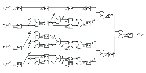
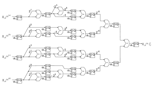
Figure 5: Final reconstruction step blocks with multi-level pipelining, for (10) and (11), respectively.

Figure 6: Final reconstruction step blocks with multi-level pipelining, for (12) and (13), respectively.

Table 2: Fast algorithms for required integer multipliers

$m$	Input: $x$; Output: $y$, where $y=m\cdot x$
669	$v_{1}=(1+2)\cdot x$ ; $v_{2}=(1-2^{3})\cdot v_{1}$ ; $y=-v_{1}-2^{5}\cdot v_{2}$
2217	$v_{1}=(1+2^{4})\cdot x$ ; $v_{2}=(1+2)\cdot x$ ; $v_{3}=v_{1}+2^{3}\cdot v_{2}$ ;
	$y=2^{7}\cdot v_{1}+v_{3}$
181	$v_{1}=(1+2)\cdot x$ ; $v_{2}=2^{3}\cdot x+v_{1}$ ; $y=2^{6}\cdot v_{1}-v_{2}$
3135	$v_{1}=(1+2)\cdot x$ ; $v_{2}=(1-2^{6})\cdot x$ ; $y=2^{10}\cdot v_{1}-v_{2}$
473	$v_{1}=(1+2^{2})\cdot x$ ; $v_{2}=x-2^{3}\cdot v_{1}$ ; $y=2^{9}\cdot x+v_{2}$
437	$v_{1}=(1+2^{2})\cdot x$ ; $v_{2}=2^{5}\cdot x-v_{1}$ ; $y=v_{1}+2^{4}\cdot v_{2}$
2399	$v_{1}=(1+2^{2})\cdot x$ ; $v_{2}=x+2^{5}\cdot v_{1}$ ; $y=2^{9}\cdot v_{1}-v_{2}$
8	$y=2^{3}\cdot x$

Finally, considering the above quantities and applying (2), the sought fixed-point representations are fully recovered. Hardware implementation of the multiplier circuits, required by the 12-bit approximations above, is accomplished by using the method of Dempster and Macleod [66, 67]. This method is known to be optimal for constant integer multiplier circuits.

In this multiplierless method, the minimum number of 2-input adders are used for each constant integer multiplier. Wired shifts that perform “costless” multiplications by powers of two are used in each constant integer multiplier. Here, an enhancement to the Dempster-Macleod method is made for the constant integer multiplier circuits: the number of adder-bits is minimized, rather than the number of 2-input adders, yielding a smaller overall design.

Accordingly, the multiplications by non powers of two shown in expressions (10)-(13) can be algorithmically implemented as described in Table 2. Fig. 5 and 6 depict the corresponding pipeline implementation. Here, the various stages of the pipelined FRS architectures are shown by having FIFO registers (consisting of parallel delay flip-flops (D-FFs)) vertically aligned in the figures. Vertically aligned D-FFs indicate the same computation point in a pipelined constant coefficient multiplication within the FRS.

4.2 FRS based on expansion factor scaling

The set of exact values given in (9) suggests further relations among those quantities. Indeed, it may be established the following relations:

$$z_{1}^{2} =4+z_{1}z_{2}, z_{2}^{2} =4-z_{1}z_{2},$$

$$z_{1}^{2}z_{2} =2\cdot(z_{1}+z_{2}), z_{1}z_{2}^{2} =2\cdot(z_{1}-z_{2}),$$

$$z_{1}^{2}z_{2}^{2} =8.$$

These identities indicate that a new design can be fostered. In fact, by substituting the above relations into (5)–(8), we have the following expressions:

$$\begin{split}{X_{i,k}}^{(a)}=&{{X_{i,k}}^{(a)}}^{(a)}+{{X_{i,k}}^{(a)}}^{(b)}z_{1}+\\ &{{X_{i,k}}^{(a)}}^{(c)}z_{2}+{{X_{i,k}}^{(a)}}^{(d)}z_{1}z_{2},\end{split}$$

$$\begin{split}{X_{i,k}}^{(b)}z_{1}=&4\cdot{{X_{i,k}}^{(b)}}^{(b)}+\left(2\cdot{{X_{i,k}}^{(b)}}^{(d)}+{{X_{i,k}}^{(b)}}^{(a)}\right)z_{1}+\\ &2\cdot{{X_{i,k}}^{(b)}}^{(d)}z_{2}+\left({{X_{i,k}}^{(b)}}^{(b)}+{{X_{i,k}}^{(b)}}^{(c)}\right)z_{1}z_{2},\end{split}$$

$$\begin{split}{X_{i,k}}^{(c)}z_{2}=&4\cdot{{X_{i,k}}^{(c)}}^{(c)}+2\cdot{{X_{i,k}}^{(c)}}^{(d)}z_{1}+\\ &\left({{X_{i,k}}^{(c)}}^{(a)}-2\cdot{{X_{i,k}}^{(c)}}^{(d)}\right)z_{2}+\\ &\left({{X_{i,k}}^{(c)}}^{(b)}-{{X_{i,k}}^{(c)}}^{(c)}\right)z_{1}z_{2},\end{split}$$

$$\begin{split}{X_{i,k}}^{(d)}z_{1}z_{2}=&8\cdot{{X_{i,k}}^{(d)}}^{(d)}+2\cdot\left({{X_{i,k}}^{(d)}}^{(b)}+{{X_{i,k}}^{(d)}}^{(c)}\right)z_{1}+\\ &2\cdot\left({{X_{i,k}}^{(d)}}^{(b)}-{{X_{i,k}}^{(d)}}^{(c)}\right)z_{2}+{{X_{i,k}}^{(d)}}^{(a)}z_{1}z_{2}.\end{split}$$

Notice that the output value $X_{i,k}$ is the summation of the above quantities. Therefore, by grouping the terms on $\{1,z_{1},z_{2},z_{1}z_{2}\}$, we can express $X_{i,k}$ by the following summation:

$$X_{i,k}={Y_{i,k}}^{(a)}+{Y_{i,k}}^{(b)}z_{1}+{Y_{i,k}}^{(c)}z_{2}+{Y_{i,k}}^{(d)}z_{1}z_{2},$$ (14)

where

$$\begin{split}{Y_{i,k}}^{(a)}=&{{X_{i,k}}^{(a)}}^{(a)}+4\cdot\left({{X_{i,k}}^{(b)}}^{(b)}+{{X_{i,k}}^{(c)}}^{(c)}\right)+\\ &8\cdot{{X_{i,k}}^{(d)}}^{(d)},\end{split}$$ (15)

$$\begin{split}{Y_{i,k}}^{(b)}=&{{X_{i,k}}^{(a)}}^{(b)}+{{X_{i,k}}^{(b)}}^{(a)}+2\cdot\left({{X_{i,k}}^{(b)}}^{(d)}+\right.\\ &\left.{{X_{i,k}}^{(c)}}^{(d)}+{{X_{i,k}}^{(d)}}^{(b)}+{{X_{i,k}}^{(d)}}^{(c)}\right),\end{split}$$ (16)

$$\begin{split}{Y_{i,k}}^{(c)}=&{{X_{i,k}}^{(a)}}^{(c)}+{{X_{i,k}}^{(c)}}^{(a)}+2\cdot\left({{X_{i,k}}^{(b)}}^{(d)}-\right.\\ &\left.{{X_{i,k}}^{(c)}}^{(d)}+{{X_{i,k}}^{(d)}}^{(b)}-{{X_{i,k}}^{(d)}}^{(c)}\right),\end{split}$$ (17)

$$\begin{split}{Y_{i,k}}^{(d)}=&{{X_{i,k}}^{(a)}}^{(d)}+{{X_{i,k}}^{(b)}}^{(b)}+{{X_{i,k}}^{(b)}}^{(c)}+\\ &{{X_{i,k}}^{(c)}}^{(b)}-{{X_{i,k}}^{(c)}}^{(c)}+{{X_{i,k}}^{(d)}}^{(a)}.\end{split}$$ (18)

Quantities ${Y_{i,k}}^{(q)}$, $q\in\{a,b,c,d\}$, require extremely simple arithmetic to be computed. These operations are represented by the combinational block in Fig. 7. We now turn to the problem of efficiently evaluate (14), which depends on $z_{1}$, $z_{2}$, and $z_{1}z_{2}$.

A possibility is to employ an expansion factor that could simultaneously scale the quantities $z_{1}$, $z_{2}$, and $z_{1}z_{2}$ into integer values. This would facilitate the usage of integer arithmetic. Such approach has been often employed by integer transform designers [68, 69]. A good exposition on this method and related schemes is found in [44, Ch. 5].

In mathematical terms, we have the following problem. Let the quantities $z_{1}$, $z_{2}$, and $z_{1}z_{2}$ form a vector $\bm{\zeta}=\begin{bmatrix}z_{1}&z_{2}&z_{1}z_{2}\end{bmatrix}^{T}$. An expansion factor [44, p. 274] is the real number $\alpha^{\ast}>1$ that satisfies the following minimization problem:

$$\alpha^{\ast}=\arg\min_{\alpha>1}\|\alpha\cdot\bm{\zeta}-\operatorname{round}(\alpha\cdot\bm{\zeta})\|,$$ (19)

where $\|\cdot\|$ is a given error measure and $\operatorname{round}(\cdot)$ is the rounding function. We adopt the Euclidean norm as the error measure. The presence of the rounding function introduces several algebraic difficulties. A closed-form solution for (19) is a non-trivial manipulation. Thus, we may resort to computational search. Clearly, additional restrictions must be imposed: a limited search space and a given precision for $\alpha$.

In the range $\alpha\in[1,256]$ with a precision of $10^{-4}$, we could find the optimal value $\alpha^{\ast}=167.2309$. Thus, we have the following scaling:

$$\alpha^{\ast}\cdot\begin{bmatrix}z_{1}\\ z_{2}\\ z_{1}z_{2}\end{bmatrix}=\begin{bmatrix}436.995521744185\ldots\\ 181.009471802748\ldots\\ 473.00054429861\ldots\end{bmatrix}\approx\begin{bmatrix}437\\ 181\\ 473\end{bmatrix}.$$

The error norm is approximately $10^{-2}$, which is very low for this type of problem.

However, notice that small values of $\alpha$ are desirable, since they could scale $\bm{\zeta}$ into small integers, which require a simple hardware design. An analysis on the sub-optimal solutions for (19) shows that $\alpha^{\prime}=4.5961$ furnishes the following scaling:

$$\alpha^{\prime}\cdot\begin{bmatrix}z_{1}\\ z_{2}\\ z_{1}z_{2}\end{bmatrix}=\begin{bmatrix}12.01031370924931\ldots\\ 4.97483482672658\ldots\\ 12.99986988195626\ldots\end{bmatrix}\approx\begin{bmatrix}12\\ 5\\ 13\end{bmatrix}.$$

In this case, the resulting integers are relatively small and the error norm is in the order of $10^{-2}$.

Now we are in position to address the computation of (14). Considering a given expansion factor $\alpha$, we can write:

$$\begin{split}X_{i,k}=\frac{1}{\alpha}&\left(\alpha\cdot{X_{i,k}}^{(a)}+m_{1}\cdot{X_{i,k}}^{(b)}+\right.\\ &\left.m_{2}\cdot{X_{i,k}}^{(c)}+m_{3}\cdot{X_{i,k}}^{(d)}\right),\end{split}$$ (20)

where $m_{1}$, $m_{2}$, and $m_{3}$ are the integer constants implied by the expansion factor $\alpha$. In particular, these constants are $\{437,181,473\}$, for $\alpha=\alpha^{\ast}$, and $\{12,5,13\}$, for $\alpha=\alpha^{\prime}$. Notice that (20) consists of a linear combination.

Because constants $m_{1}$, $m_{2}$, and $m_{3}$ are integers, associate multiplications can be efficiently implemented in hardware. Considering common subexpression elimination (CSE), these multiplications are reduced to additions and shift operations, requiring minimal amount of hardware resources. For the set $\{437,181,473\}$, we have the following CSE manipulation:

$$437\cdot{Y_{i,k}}^{(b)}+ 181\cdot{Y_{i,k}}^{(c)}+473\cdot{Y_{i,k}}^{(d)}=$$

$$473\cdot\left({Y_{i,k}}^{(b)}+{Y_{i,k}}^{(c)}+{Y_{i,k}}^{(d)}\right)-$$

$$36\cdot\left({Y_{i,k}}^{(b)}+{Y_{i,k}}^{(c)}\right)-$$

$$256\cdot{Y_{i,k}}^{(c)}.$$

This computation requires only eight additions. Analogously, for the set $\{12,5,13\}$, CSE yields:

$$12\cdot{Y_{i,k}}^{(b)}+ 5\cdot{Y_{i,k}}^{(c)}+13\cdot{Y_{i,k}}^{(d)}=$$

$$8\cdot\left({Y_{i,k}}^{(b)}+{Y_{i,k}}^{(d)}\right)+$$

$$4\cdot\left({Y_{i,k}}^{(b)}+{Y_{i,k}}^{(c)}+{Y_{i,k}}^{(d)}\right)+$$

$${Y_{i,k}}^{(d)}+{Y_{i,k}}^{(c)}.$$

Five additions are necessary. Above calculations are represented by the integer coefficient block in Fig. 7.

The remaining multiplication in (20) is the one by $\alpha$, which can be implemented according to the Booth encoding representation. Table 3 brings the required Booth encoding for $\alpha^{\ast}=167.2309$ and $\alpha^{\prime}=4.5961$.

Table 3: Booth encoding of the expansion factors $\alpha$

$\alpha$	Representation
4.5961	$2^{2}+2^{-1}+2^{-4}+2^{-5}+2^{-9}$
167.2309	$2^{7}+2^{5}+2^{3}-2^{0}+2^{-2}-2^{-6}-2^{-8}$

The global multiplication by $1/\alpha$ is not problematic. Indeed, it can be embedded into subsequent signal processing stages after the DCT operation. Typically, it is absorbed into the quantizer. This approach has been employed in several DCT architectures [70, 71, 69].

Fig. 7 depicts the full block diagram of the discussed computing scheme. Eight separate instances of this block are necessary to compute coefficients $X_{i,0}$ to $X_{i,7}$, for each $i$.

Figure 7: Block diagram of the proposed AI decoding based on expansion factors.

5 On-FPGA Test and Measurement

Table 4: Success rates of the DCT coefficient computation for various fixed-point bus widths $L$ and tolerance levels

				Percentage Tolerance
Design	FRS Method		$L$	10%	5%	1%	0.1%	0.05%	0.01%	0.005%
1	Dempster-Macleod		4	99.9672	99.9203	99.6422	96.3563	92.7109	64.8406	42.1719
2			8	99.9719	99.9344	99.6047	96.3250	92.7031	64.7313	41.9016
3	Expansion factor	$\{12,5,13\}$	4	99.1844	98.2944	91.6822	55.1811	45.0667	30.6922	22.8633
4			8	99.1289	98.2944	91.4978	55.0900	45.0289	30.7122	22.8844
5		$\{437,181,473\}$	4	99.9900	99.9822	99.9178	99.1111	98.2000	91.0667	83.1244
6			8	99.9589	99.9511	99.8733	99.0389	98.1278	90.9867	83.1767

Figure 8: Resource utilization, speed of operation, and power consumption of the DCT designs given in Table 4 on Xilinx Virtex-6 XC6VLX240T FPGA for input fixed-point wordlength $L=4$.

Figure 9: Resource utilization, speed of operation, and power consumption of the DCT designs given in Table 4 on Xilinx Virtex-6 XC6VLX240T FPGA for input fixed-point wordlength $L=8$.

Six designs were implemented on Xilinx ML605 evaluation kit which is populated with a a Xilinx Virtex-6 XC6VLX240T device. The designs included the three implementations of the 2D 8$\times$8 Arai AI DCT architecture with the two types of FRS described in Section 4 for fixed-point 4- and 8-bit wordlengths. Two versions of the expansion factor FRSs are provided, corresponding to expansion factors $\alpha^{\prime}=4.5941$ and $\alpha^{*}=167.2309$, resulting in 6 designs in total. The proposed designs are listed in Table 4.

The JTAG interface was used to input the test 8$\times$8 2-D DCT arrays to the device from the Matlab workspace. Then the measured outputs were returned to the Matlab workspace via the same interface. Hardware computed coefficients were compared to its numerical evaluation furnished by Matlab signal processing toolbox.

5.1 On-chip Verification using Success Rates

As a figure of merit, we considered the success rate defined as the percentage of coefficients which are within the error limit of $\pm e\,\%$. For $e=\{0.005,0.01,0.05,0.1,1,5,10\}$, the success rates were measured as given in the Table 4. Input wordlengths $L$ was set to 4 or 8 bits. The 8-bit size is the typical video processing configuration. The proposed AI architectures enjoy overflow-free bit-growth at each stage throughout the AI encoded structure thereby ensuring that all sources of error are at the FRS and there only. Results show that the FRS based on the expansion factor approach for $\{437,181,473\}$ (Designs 5 and 6) offers a significant improvement in accuracy when compared to remaining FRS architectures.

5.2 FPGA Resource Consumption

The resource consumption of the proposed architectures on Xilinx Virtex-6 XC6VLX240T device are shown in Fig. 8 for $L=4~{}\text{bits}$. Fig. 9 brings analogous information for $L=8~{}\text{bits}$. Here, FPGA resources are measured in terms of slices, slice registers, and slice look-up-tables (LUTs). Designs 3 and 4, which use the FRS based on the expansion factor approach for $\{12,5,13\}$, consumed the least resources in the device and has the worst accuracy of the three designs (Table 4). Moreover, even though Designs 5 and 6 (FRS based on expansion factor approach for $\{437,181,473\}$) possesses superior accuracy when compared to Designs 1 and 2 (FRS based on Dempster-Macleod method), they consume less hardware resources. Overall the FRS step of the proposed architectures require a considerable amount of area when compared to the AI steps of the architecture.

5.3 Clock Speed, Block Rate, Frame Rate

Table 5: Frame rates and block rates achieved by the implemented designs for a video of resolution 1920$\times$1080

Design	Freq. (MHz)	Block rate (MHz)	Frame rate (Hz)
1	130.410	16.30	503.08
2	123.120	15.39	475.00
3	309.855	38.73	1195.37
4	300.391	37.55	1158.95
5	312.402	39.05	1205.25
6	307.787	38.47	1187.35

Frame rates and block rates achieved by the implemented designs for video at resolution 1920$\times$1080 is shown in Table 5. The design having the best throughput was Design 5, which operates on 4-bit inputs. In Design 5, the maximum 8$\times$8 2-D DCT block rate is 39.05 MHz for a 312.402 MHz clock. Assuming an input video resolution of 1920$\times$ 1080 pixels per frame, we obtained a real-time computation of the 2-D 8$\times$8 DCT at 1205.25 frames per second. In Design 6, we describe the common 8-bit input case, where the clock is now slightly reduced to 307.787 MHz, yielding an $8\times 8$ block rate of 38.787 MHz, and a frame rate of 1187.35 frames per second for the same image size as above. In all cases, if the 2-D DCT core is eventually embedded in a real-time video processor, the pixel rate is eight fold the clock frequency of the DCT core (due to the downsampling by eight in the signal flow graph). For example, a potential pixel rate of $\approx$2.499 GHz and $\approx$2.462 GHz, for Designs 5 and 6, may be possible.

5.4 Xilinx Power Consumption and Critical Path

The total power consumption of FPGA circuits consist of the sum of dynamic and quiescent power consumptions. Both estimated dynamic and quiescent power consumptions obtained from the design tools for the Xilinx Virtex-6 XC6VLX240T device are provided in Fig. 8 and Fig. 9.

5.5 Area-Time Complexity Metrics

Estimates for VLSI area-time complexity metrics are provided for all designs are given in Fig. 8 ($L=4$) and Fig. 9 ($L=8$), respectively. In general, the area-time metric measures complexity of VLSI circuits where chip real-estate is important over speed, while metric area-time² is used often for VLSI circuits where speed is of paramount concern. We provide both metrics to offer a broad overview of the area-time complexity levels present in the proposed architectures as a function of input size and choice of FRS algorithm.

The architectures are free of general purpose multipliers.

5.6 Overall Comparison with Existing Architectures

Fixed point VLSI implementations that are directly comparable to the proposed architecture are compared in detail in Table 5.6. Table 5.6 brings comparisons to AI-based architectures. For brevity and without loss of generality, we chose designs 2 and 6 for the purpose of comparison. These are aimed at 8-bit input signals and are examples of the Dempster-Macleod and expansion factor FRS algorithms. A synopsis of both fixed-point and AI-based 2D-DCT circuits under comparison in Tables  5.6 and  5.6 was provided in Section 2.

[b]

Table 6: Comparison of the proposed implementation with published fixed point implementations

	Lin et al. [32]	Shams et al. [31]	Madisetti et al. [17]	Guo et al. [29]	Tumeo et al. [28]	Sun et al. [30]	Chen et al. [22]	Proposed architectures
								Design 2	Design 6
Measured results	No	No	No	No	No	No	No	Yes	Yes
Structure	Single 2-D DCT	Two 1-D DCT +TMEM$\dagger$	Single 1-D DCT +TMEM$\dagger$	Single 1-D DCT +TMEM$\dagger$	Single 1-D DCT +TMEM$\dagger$	Two 1-D DCT +TMEM$\dagger$	Single 1-D DCT +TMEM$\dagger$	See Fig. 3	See Fig. 3
Multipliers	1	0	7	0	4	0	0	0	0
Operating frequency (MHz)	100	N/A	100	110	107	149	167	123.12	307.79
8$\times$8 Block rate
$\times 10^{6}\mathrm{s}^{-1}$	1.5625	N/A	1.562	3.4375	1.3375	2.328	2.609	15.39$\ast$	38.625$\ast$
Pixel rate
$\times 10^{6}\mathrm{s}^{-1}$	100	N/A	100	220	85.6	149	167	984.96$\ddagger$	2462.32$\ddagger$
Implementation technology	0.13$\mu$m CMOS	N/A	0.8$\mu$m CMOS	0.35$\mu$m CMOS	Xilinx XC2VP30	Xilinx XC2VP30	0.18$\mu$m CMOS	Xilinx XC6VLX240T	Xilinx XC6VLX240T
Coupled quantization noise	Yes	Yes	Yes	Yes	Yes	Yes	Yes	No	No
Independently adjustable precision	No	No	No	No	No	No	No	Yes	Yes

• Row column transpose buffer.

• Block rate$=F_{clock}/8$.

• Pixel rate $=F_{s}$.

[b]

Table 7: Comparison of the proposed implementation with published algebraic integer implementations

	Nandi et al. [56]	Jullien et al. [50]	Wahid et al. [55]	Proposed architectures
				Design 2	Design 6
Measured
results	No	No	No	Yes	Yes
Structure	Single 1-D DCT +Mem. bank	Two 1-D DCT +Dual port RAM	Two 1-D DCT +TMEM$\dagger$	See Fig. 3	See Fig. 3
Multipliers	0	0	0	0	0
Exact 2D AI computation	No	No	No	Yes	Yes
Operating
frequency
(MHz)	N/A	75	194.7	123.12	307.79
8$\times$8 Block rate $\times 10^{6}\mathrm{s}^{-1}$	7.8125	1.171	3.042	15.39$\ast$	38.625$\ast$
Pixel rate
$\times 10^{6}\mathrm{s}^{-1}$	125	75	194.7	984.96$\ddagger$	2462.32$\ddagger$
Implementation technology	Xilinx XC5VLX30	0.18$\mu$m
CMOS	0.18$\mu$m
CMOS	Xilinx XC6VLX240T	Xilinx XC6VLX240T
Coupled quantization
noise	Yes	Yes	Yes	No	No
Independently adjustable
precision	No	No	No	Yes	Yes
FRS between row-column stages	No	Yes	Yes	No	No

• Row column transpose buffer.

• Block rate$=F_{clock}/8$.

• Pixel rate $=F_{s}$.

6 Conclusions

A time-multiplexed systolic-array hardware architecture is proposed for the real-time computation of the bivariate AI encoded 2-D Arai DCT. The architecture is the first 2-D AI encoded DCT hardware that operates completely in the AI domain. This not only makes the proposed system completely multiplier-free, but also quantization free up to the final output channels.

Our architecture employs a novel AI-TB, which facilitates real-time data transposition. The 2-D separable DCT operation is entirely performed in the AI domain. Indeed, the architecture does not have intermediate FRS sections between the column- and row-wise AI-based Arai DCT operations. This makes the quantization noise only appear at the final output stage of the architecture: the single FRS section.

The location of the FRS at the final output stage results in the complete decoupling of quantization noise between the 64 parallel coefficient channels of the 2-D DCT. This fact is noteworthy because it enables the independent selection of precision for each of the 64 channels without having any effect on the speed, power, complexity, or noise level of the remaining channels.

Two algorithms for the FRS are proposed, numerically optimized, analyzed, hardware implemented, and tested with the proposed 2-D AI encoded section. The architectures are physically implemented for input precision of 4 and 8 bits, and fully verified on-chip. Of particular relevance is the commonly required 8-bit realization, which is operational at a clock frequency of 307.787 MHz on a Xilinx Virtex-6 XC6VLX240T FPGA device (see Design 6). This implies a $8\times 8$ block rate of 38.47 MHz and a potential pixel rate of $\approx$2.462 GHz if the proposed 2-D DCT core is embedded in a real-time video processing system. The frame rate for standard HD video at $1920\times 1080$ resolution is $\approx$1187.35 Hz assuming 8-bit input words and core clock frequency of 307.787 MHz.

The proposed architecture achieves complete elimination of quantization noise coupling between DCT coefficients, which is present in published 2-D DCT architectures based on both fixed-point arithmetic as well as row-column 8-point Arai DCT cores that have FRS sections between row- and column-wise transforms. The proposed designs allows each of the 64 coefficients to be computed at 64 different precision levels, where each choice of precision only affects that particular coefficient. This allows full control of the 2-D DCT computation to any degree of precision desired by the designer.

Acknowledgments

This work was partially supported by CNPq and FACEPE.

References

- [1] H.-Y. Lin and W.-Z. Chang, “High dynamic range imaging for stereoscopic scene representation,” in Proceedings of the 16th IEEE International Conference on Image Processing (ICIP), Nov. 2009, pp. 4305–4308.
- [2] W.-C. Kao, “High dynamic range imaging by fusing multiple raw images and tone reproduction,” IEEE Transactions on Consumer Electronics, vol. 54, no. 1, pp. 10–15, Feb. 2008.
- [3] P. Carrillo, H. Kalva, and S. Magliveras, “Compression independent reversible encryption for privacy in video surveillance,” EURASIP Journal on Information Security, vol. 2009, pp. 1–13, 2009.
- [4] C.-F. Chiasserini and E. Magli, “Energy consumption and image quality in wireless video-surveillance networks,” in Proceedings of the 13th IEEE International Symposium on Personal, Indoor and Mobile Radio Communications, vol. 5, Sep. 2002, pp. 2357–2361.
- [5] E. Magli and D. Taubman, “Image compression practices and standards for geospatial information systems,” in Proceedings of the 2003 IEEE International Geoscience and Remote Sensing Symposium, vol. 1, Jul. 2003, pp. 654–656.
- [6] M. Bramberger, J. Brunner, B. Rinner, and H. Schwabach, “Real-time video analysis on an embedded smart camera for traffic surveillance,” in Proceedings of the 10th IEEE Real-Time and Embedded Technology and Applications Symposium, May 2004, pp. 174–181.
- [7] T. Tada, K. Cho, H. Shimoda, T. Sakata, and S. Sobue, “An evaluation of JPEG compression for on-line satellite images transmission,” in Proceedings of the International Geoscience and Remote Sensing Symposium (IGARSS), Aug. 1993, pp. 1515–1518.
- [8] A. S. Dawood, J. A. Williams, and S. J. Visser, “On-board satellite image compression using reconfigurable FPGAs,” in Proceedings of the IEEE International Conference on Field-Programmable Technology, Dec. 2002, pp. 306–310.
- [9] J. Schiewe, “Effect of lossy data compression techniqes on geometry and information content of satellite imagery,” in Proceedings of the ISPRS Commission IV Symposium on GIS - Between isions and Applications, D. Fritsch, M. Englich, and M. Sester, Eds., vol. 32, Stuttgart, Germany, 1998.
- [10] B. Bennett, C. Dee, and C. Meyer, “Emerging methodologies in encoding airborne sensor video and metadata,” in Proceedings of the 2009 IEEE Military Communications Conference, Oct. 2009, pp. 1–6.
- [11] J. Wang and Y. Song, “Hardware design of video compression system in the UAV based on the ARM technology,” in Proceedings of the 2009 International Symposium on Computer Network and Multimedia Technology, Jan. 2009, pp. 1–4.
- [12] B. Bennett, C. Dee, M.-H. Nguyen, and B. Hamilton, “Operational concepts of MPEG-4 H.264 for tactical DoD applications,” in Proceedings of the IEEE Military Communications Conference, vol. 1, Oct. 2005, pp. 155–161.
- [13] S. Marsi, G. Impoco, A. Ukovich, S. Carrato, and G. Ramponi, “Video enhancement and dynamic range control of HDR sequences for automotive applications,” EURASIP Journal on Advances in Signal Processing, vol. 2007, pp. 1–9, 2007.
- [14] I. F. Akyildiz, T. Melodia, and K. R. Chowdhury, “A survey on wireless multimedia sensor networks,” Computer Networks, vol. 51, no. 4, pp. 921–960, 2007.
- [15] R. Westwater and B. Furht, Real-time video compression: techniques and algorithms, ser. Kluwer international series in engineering and computer science. Kluwer, 1997.
- [16] T. Suzuki and M. Ikehara, “Integer DCT based on direct-lifting of DCT-IDCT for lossless-to-lossy image coding,” IEEE Transactions on Image Processing, vol. 19, no. 11, pp. 2958–2965, Nov. 2010.
- [17] A. Madisetti and A. N. Willson, “A 100 MHz 2-D DCT-IDCT processor for HDTV applications,” IEEE Transactions on Circuits and Systems for Video Technology, vol. 5, no. 2, pp. 158–165, Apr. 1995.
- [18] D. F. Chiper, M. Swamy, M. O. Ahmad, and T. Stouraitis, “Systolic algorithms and a memory-based design approach for a unified architecture for the computation of DCT-DST-IDCT-IDST,” IEEE Transactions on Circuits and Systems I: Regular Papers, vol. 52, no. 6, pp. 1125–1137, Jun. 2005.
- [19] P. K. Meher and M. N. S. Swamy, “New systolic algorithm and array architecture for prime-length discrete Fourier transform,” IEEE Transactions on Circuits and Systems II: Express Briefs, vol. 54, no. 3, pp. 262–266, Mar. 2007.
- [20] T.-Y. Sung, Y.-S. Shieh, and H.-C. Hsin, “An efficient VLSI linear array for DCT/IDCT using subband decomposition algorithm,” Mathematical Problems in Engineering, vol. 2010, pp. 1–21, 2010.
- [21] H. Huang, T.-Y. Sung, and Y.-S. Shieh, “A novel VLSI linear array for 2-D DCT-IDCT,” in Proceedings of 2010 3rd International Congress on Image and Signal Processing (CISP’2010). IEEE, 2010, pp. 3686–3690.
- [22] Y.-H. Chen and T.-Y. Chang, “A high performance video transform engine by using space-time scheduling stratergy,” IEEE Transactions on Very Large Scale Integration (VLSI) Systems, Forthcoming in 2011.
- [23] P. K. Meher, J. C. Patra, and A. P. Vinod, “A 2-D systolic array for high-throughput computation of 2-D discrete Fourier transform,” in Proceedings of IEEE Asia Pacific Conference on Circuits and Systems (APCCAS’2006), 2006.
- [24] P. K. Meher, “Unified DA-based parallel architecture for compting the DCT and the DST,” in Proceedings of the 5th IEEE International Conference on Information, Communications, and Signal Processing, 2005, pp. 1278–1282.
- [25] S. Nayak and P. Meher, “3-dimensional systolic architecture for parallel VLSI implementation of the discrete cosine transform,” IEE Proc.- Circuits Devices and Syst., vol. 143, no. 5, pp. 255–258, Oct. 1996.
- [26] P. K. Meher, “Highly concurrent reduced-complexity 2-D systolic array for discrete Fourier transform,” IEEE Signal Processing Letters, vol. 13, no. 8, pp. 481–484, Aug. 2006.
- [27] P. K. Meher and J. Patra, “A new convolutional formulation of discrete cosine transform for systolic implementation,” in Proceedings of IEEE International Conference on Information, Communications, and Systolic Implementation, 2007, pp. 1–4.
- [28] A. Tumeo, M. Monchiero, G. Palermo, F. Ferrandi, and D. Sciuto, “A pipelined fast 2D-DCT accelerator for FPGA-based SoCs,” in Proceedings of IEEE Computer Society Annual Symposium on VLSI (ISVLSI’07), 2007.
- [29] J.-I. Guo, R.-C. Ju, and J.-W. Chen, “An efficient 2-D DCT/IDCT core design using cyclic convolution and adder-based realization,” IEEE Transactions on Circuits and Systems for Video Technology, vol. 14, no. 4, pp. 416–428, Apr. 2004.
- [30] C.-C. Sun, P. Donner, and J. Gotze, “Low-complexity multi-purpose IP core for quantized discrete cosin and integer transform,” in In Proceedings of 2009 IEEE Intl. Symp. on Circuits and Systems (ISCAS’09), 2009, pp. 3014–3017.
- [31] A. M. Shams, A. Chidanandan, W. Pan, and M. A. Bayoumi, “NEDA: A low-power high-performance DCT architecture,” IEEE Trans on Signal Processing, vol. 3, no. 3, pp. 955–964, Mar. 2006.
- [32] C.-T. Lin, Y.-C. Yu, and L.-D. Van, “Cost-effective triple-mode reconfigurable pipeline FFT/IFFT/2-D DCT processor,” IEEE Transactions on Very Large Scale Integration (VLSI) Systems, vol. 16, no. 8, pp. 1058–1071, Aug. 2008.
- [33] C.-Y. Huang, L.-F. Chen, and Y.-K. Lai, “A high-speed 2-D transform architecture with unique kernel for multi-standard video applications,” in Proceedings of IEEE 2008 Intlernational Symposium on Circuits and Systems (ISCAS’2008), 2008, pp. 21–24.
- [34] A. V. Oppenheim and C. J. Weinstein, “Effects of finite register length in digital filtering and the fast Fourier transform,” Proceedings of the IEEE, vol. 60, no. 8, pp. 957–976, Aug. 1972.
- [35] K. Ihsberner, “Roundoff error analysis of fast DCT algorithms in fixed point arithmetic,” Numerical Algorithms, vol. 46, pp. 1–22, 2007. [Online]. Available: http://dx.doi.org/10.1007/s11075-007-9123-1
- [36] V. S. Dimitrov, G. A. Jullien, and W. C. Miller, “A new DCT algorithm based on encoding algebraic integers,” in Proceedings of the 1998 IEEE International Conference on Acoustics, Speech and Signal Processing, vol. 3, May 1998, pp. 1377–1380.
- [37] K. Wahid, “Error-free implementation of the discrete cosine transform,” Ph.D. dissertation, University of Calgary, 2010.
- [38] R. Baghaie and V. Dimitrov, “Systolic implementation of real-valued discrete transforms via algebraic integer quantization,” Computers and Mathematics with Applications, vol. 41, pp. 1403–1416, 2001.
- [39] H. A. Peterson, A. J. Ahumada, and A. B. Watson, “The visibility of DCT quantization noise,” SID International Symposium Digest Of Technical Papers, vol. 24, p. 942, 1993.
- [40] M. A. Robertson and R. L. Stevenson, “DCT quantization noise in compressed images,” IEEE Transactions on Circuits and Systems for Video Technology, vol. 15, no. 1, pp. 27– 38, Jan. 2005.
- [41] V. Dimitrov, K. Wahid, and G. Jullien, “Multiplication-free 88 2D DCT architecture using algebraic integer encoding,” IEE Electronics Letters, vol. 40, no. 20, pp. 1310–1311, 2004.
- [42] V. Dimitrov and K. Wahid, “On the error-free computation of fast cosine transform,” International Journal: Information Theories and Applications, vol. 12, no. 4, pp. 321–327, 2005.
- [43] Y. Arai, T. Agui, and M. Nakajima, “A fast DCT-SQ scheme for images,” IEICE Transactions, vol. E71-E, no. 11, pp. 1095–1097, 1988.
- [44] V. Britanak, P. Yip, and K. R. Rao, Discrete Cosine and Sine Transforms. Academic Press, 2007.
- [45] “Xilinx, inc. corporate website,” 2011. [Online]. Available: http://www.xilinx.com/
- [46] J. H. Cozzens and L. A. Finkelstein, “Range and error analysis for a fast Fourier transform computed over ,” IEEE Transactions on Information Theory, vol. IT-33, no. 4, pp. 582–590, Jul. 1987.
- [47] M. Fu, V. S. Dimitrov, and G. Jullien, “An efficient technique for error-free algebraic-integer encoding for high performance implementation of the DCT and IDCT,” in Proceedings of the IEEE 2001 International Symposium on Circuits and Systems (ISCAS’01), 2001.
- [48] M. Fu, G. Jullien, V. S. Dimitrov, M. Ahmadi, and W. Miller, “Implementation of an error-free DCT using algebraic integers,” in Proceedings of the Micronet Annual Workshop, 2002.
- [49] ——, “The application of 2D algebraic integer encoding to a DCT IP core,” in Proceedings of the 3rd IEEE International Workshop on System-on-Chip for Real-Time Applications, Calgary, AB, CA, 2002, pp. 66–69.
- [50] M. Fu, G. A. Jullien, V. S. Dimitrov, and M. Ahmadi, “A Low-Power DCT IP Core based on 2D Algebraic Integer Encoding,” in Proceedings of the 2004 International Symposium on Circuits and Systems, 2004 (ISCAS ’04), vol. 2, May 2004, pp. 765–768.
- [51] M. Fu, G. Jullien, and M. Ahmadi. (2004, Feb.) Algebraic integer encoding and applications in discrete cosine transform. Online. Gennum Presentation by Dept. ECE, University of Windsor, Canada. [Online]. Available: http://www.docstoc.com/docs/74259941/Algebraic-Integer-Encoding-and-Applications-in-Discrete-Cosine
- [52] K. Wahid, S. B. Ko, and V. S. Dimitrov, “Area and power efficient video compressor for endoscopic capsules,” in Proceedings of 4th International Conference on Biomedical Engineering, Kuala Lumpur, Jun. 2008.
- [53] K. Wahid, “An efficient IEEE-compliant 88 Inv-DCT architecture with 24 adders,” IEEE Transactions on Electronics, Information and Systems, vol. 131, pp. 1081–1082, 2011.
- [54] T. H. Khan and K. A. Wahid, “Lossless and low-power image compressor for wireless capsule endoscopy,” VLSI Design, vol. 2011, p. 12, 2011.
- [55] K. A. Wahid, M. Martuza, M. Das, and C. McCrosky, “Efficient hardware implementation of integer cosine transforms for multiple video codecs,” Journal of Real-Time Processing, pp. 1–8, Jul. 2011.
- [56] S. Nandi, K. Rajan, and P. Biswas, “Hardware implementation of DCT quantization block using multiplication and error-free algorithm,” in 2009 IEEE TENCON Region 10, 2009, pp. 1–5.
- [57] G. H. Hardy and E. M. Wright, An Introduction to the Theory of Numbers, 4th ed. London: Oxford University Press, 1975.
- [58] M. E. Pohst, Computational Algebraic Number Theory. Basel, Switzerland: Birkhäuser Verlag, 1993.
- [59] H. Pollard and H. G. Diamond, The Theory of Algebraic Numbers, 2nd ed., ser. The Carus Mathematical Monographs. The Mathematical Association of America, 1975, no. 9.
- [60] J. H. Cozzens and L. A. Finkelstein, “Computing the discrete Fourier transform using residue number systems in a ring of algebraic integer,” IEEE Transactions on Information Theory, vol. IT-31, no. 5, pp. 580–588, Sep. 1985.
- [61] A. Madanayake, R. J. Cintra, D. Onen, V. S. Dimitrov, and L. T. Bruton, “Algebraic integer based 88 2-D DCT architecture for digital video processing,” in Proceedings of the IEEE 2011 International Symposium on Circuits and Systems (ISCAS’2011), May 2011.
- [62] R. E. Blahut, Fast Algorithms for Signal Processing, Cambridge, UK, 2010.
- [63] V. Dimitrov, G. A. Jullien, and W. C. Miller, “Eisenstein residue number system with applications to DSP,” in Proceedings of the 40th Midwest Symposium on Circuits and Systems, 1997.
- [64] K. Wahid, V. Dimitrov, and G. Jullien, “Error-free computation of 88 2D DCT and IDCT using two-dimensional algebraic integer quantization,” in Proceedings of the 17th IEEE Symposium on Computer Arithmetic. IEEE Computer Society, Jun. 2005, pp. 214–221.
- [65] U. Meyer-Base and F. Taylor, “Optimal algebraic integer implementation with application to complex frequency sampling filters,” IEEE Transactions on Circuits and Systems II: Analog and Digital Signal Processing, vol. 48, no. 11, pp. 1078–1082, 2001.
- [66] A. G. Dempster and M. D. Macleod, “Constant integer multiplication using minimum adders,” IEE Proceedings - Circuits, Devices and Systems, vol. 141, no. 5, pp. 407–413, Oct. 1994.
- [67] O. Gustafsson, A. G. Dempster, K. Johansson, M. D. Macleod, and L. Wanhammar, “Simplified design of constant coefficient multipliers,” Circuits, Systems, and Signal Processing, vol. 25, no. 2, pp. 225–251, Apr. 2006.
- [68] G. Plonka, “A global method for invertible integer DCT and integer wavelet algorithms,” Applied and Computational Harmonic Analysis, vol. 16, no. 2, pp. 79–110, Mar. 2004.
- [69] R. J. Cintra and F. M. Bayer, “A DCT approximation for image compression,” IEEE Signal Procesing Letters, vol. 18, no. 10, pp. 579–583, Oct. 2011.
- [70] S. Bouguezel, M. O. Ahmad, and M. N. S. Swamy, “Low-complexity 88 transform for image compression,” Electronics Letters, vol. 44, no. 21, pp. 1249–1250, Sep. 2008.
- [71] ——, “A low-complexity parametric transform for image compression,” in Proceedings of the 2011 IEEE International Symposium on Circuits and Systems, 2011.