Nonconforming finite element method applied to the driven cavity problem

Abstract

A cheapest stable nonconforming finite element method is presented for solving the incompressible flow in a square cavity without smoothing the corner singularities. The stable cheapest nonconforming finite element pair based on $P_{1}\times P_{0}$ on rectangular meshes [28] is employed with a minimal modification of the discontinuous Dirichlet data on the top boundary, where $\widetilde{{\mathscr{P}}_{0}^{h}}$ is the finite element space of piecewise constant pressures with the globally one-dimensional checker-board pattern subspace eliminated. The proposed Stokes elements have the least number of degrees of freedom compared to those of known stable Stokes elements. Three accuracy indications for our elements are analyzed and numerically verified. Also, various numerous computational results obtained by using our proposed element show excellent accuracy.

1 Introduction

The lid driven square cavity has been one of the most popular benchmark problems for new numerical methods for the incompressible Navier-Stokes equations in terms of accuracy, numerical efficiency and so on. To refer only few see [4, 8, 18, 17], for instance, and the references therein. The presence of singularities at the upper corners of the cavity is the source of numerical difficulties for solving the cavity flow problem. It is usually erroneous to use high-order methods without handling the corner singularities due to the Gibbs phenomenon. Many studies have been carried out to overcome this difficulty. Barragy and Carey [6] used a $p$-version finite element formulation ($p\geq 6$) combined with a strongly graded and refined mesh to handle the corner singularities. Other studies change the boundary condition to overcome this difficulty: see, for instance, [20, 33, 32, 21], and the references therein. The latter approach are coined as the so-called regularized lid driven cavity problem. The constant boundary condition for velocity is replaced by a function that vanishes at the upper corners of cavity [20, 33]. Botella and Peyret [8] solved a regularized cavity problem by using a subtraction method of the leading terms from the asymptotic expansion of the solution of the Navier-Stokes equations in the vicinity of the corners, where the velocity is discontinuous. Sahin and Owens [32] inserted leaks across the heights of the finite volumes at the corners between the lid and the vertical walls to handle the corner singularities. Many studies reported that in the critical Reynolds number range $[7000,8500]$ Hopf bifurcations occur for the lid driven square cavity problem [4, 18, 20, 33]. Bruneau and Saad [9] revisited the issue of bifurcation using third–order time discretization schemes with the $5000\times 5000$ finite difference spatial discretizations. They observed the first bifurcation occurs between $Re=8000$ and $Re=8050.$ Guermond and Minev [24] reported three–dimensional benchmark solutions using a direction splitting method introduced in [23, 22]. They also provided two–dimensional solutions, which are correct up to at least three digits, for $Re=1000$ using the uniform $5000\times 5000$ MAC stencil. Instead of the square domain, Glowinski et al. [21] considered a semi-circular cavity-driven flow with a special time-dependent regularization on the Dirichlet data at the two corners: they observed Hopf bifurcations around $Re=6600$, which is smaller than the case of square domain, using an iso-parametric variant of the Bercovier-Pironneau element [7] introduced in [20].

The purpose of the current paper is to try to solve the lid driven square cavity problem without any regularization at the corners, employing nonconforming finite element pairs whose degrees of freedom and implementation are as cheap as possible. As the nonconforming elements use the values at the midpoints of edges as DOFs, instead of those at the vertices, the discontinuity singularities at the corners are naturally treated without any regularization. Our nonconforming finite element pairs are based on the two stable nonconforming finite element pairs on uniform square meshes [28] introduced for the stationary incompressible Stokes problem. The two pairs are briefly described as follows: The first of them uses the $P_{1}$-nonconforming quadrilateral element [30] for the approximation of the velocity field, componentwise, while the pressure is approximated by a subspace of the piecewise constant functions whose dimension is two less than the number of squares in the mesh. The second of them is a one-dimensional modification of the above finite element pairs to both velocity and pressure spaces: the velocity space is enriched by a globally one-dimensional DSSY(Douglas-Santos-Sheen-Ye)-type bubble function [15, 11, 26] while the pressure space is the subspace of the piecewise constant functions whose dimension is one less than the number of squares in the mesh in order to fulfill the mean-zero property. The stability and optimal convergence results for these element pairs applied to the stationary Stokes equations with the homogeneous Dirichlet boundary condition can be found in [28].

In order to treat the inhomogeneous lid-driven Dirichlet boundary condition, we modified the above elements [28] as follows. The boundary condition on the interior of the top boundary is handled as usual, but the corner boundary condition is specially treated at the two end elements on the top by adding two local DSSY-type bubble functions whose values at the midpoints of top boundary parts to be $(1,0)^{t}$ and at the midpoint of the other boundary parts to be $(0,0)^{t}$. Indeed, since nonconforming finite element methods can avoid vertex values degrees of freedom, the boundary values at the top left and right corners are not required. Thus, one can solve the driven cavity problem without any regularization of the boundary condition (3).

We note that the above modified finite elements have the smallest DOFs and are easiest to implement among the finite element space pairs that fetch all non-spurious piecewise constant pressure fields. Moreover, our finite element methods yield nearly divergence free velocity fields. Indeed, $\int_{\Omega}|\nabla\cdot\,{\mathbf{v}}_{h}|\,d\mathbf{x}=\mathscr{O}(h^{3})$, which is good indication of numerical solver. The $\mathscr{O}(h^{3})$ factor arises from the inhomogeneous boundary data (the finite element pairs introduced in [28] for the homogeneous boundary condition yield exactly divergence free velocity approximation.) Another indication of superiority of our element is that our methods gives substantially smaller volumetric flow rates across horizontal and vertical line sections [5] than other methods by a factor of two. They are reported in §5.

The plan of our presentation of this paper is as follows. In the next section the lid-driven cavity problem is briefly described. With a brief review on the $P_{1}$-nonconforming quadrilateral element, a detailed description and implementation of our finite element methods are given in §3. Three accuracy indications of our numerical solutions are analyzed in §4. Some numerical results are presented §5 with comparison to the results of other methods. The last section concludes our presentation.

2 Problem formulation

Let $\Omega=(0,1)^{2}$ be the square cavity. Consider the steady-state incompressible Navier-Stokes equations in dimensionless form:

$$-\nu\triangle\mathbf{u}+(\mathbf{u}\cdot\nabla)\mathbf{u}+\nabla p =\mathbf{0}\qquad\text{in}\;\Omega,$$ (1)

$$\nabla\cdot\,\mathbf{u} =0\qquad\text{in}\;\Omega,$$

with the Dirichlet boundary condition

$$\mathbf{u}=\mathbf{g}\quad\text{on}\;\Gamma\quad\text{with}\;\int_{\Gamma}{\boldsymbol{\nu}}\cdot\mathbf{g}\operatorname{\,d{s}}=0.$$ (2)

Here, $\mathbf{u}$ and $p$ denote the flow velocity and pressure, $\nu$ the fluid kinetic viscosity, $\Gamma$ the boundary of $\Omega$, and ${\boldsymbol{\nu}}$ the unit outward normal vector to $\Omega$. Here, and in what follows, bold faces will denote the two-dimensional vectors, functions, and function spaces. For the driven cavity problem, suppose that the Dirichlet data is given by

$$\mathbf{g}(x,y)=\left\{\begin{aligned} &(1,0)^{t}\;\text{ if }0<x<1\;\text{ and }\;y=1,\\ &\text{arbitrary }\;\text{ if }x=0,1\;\text{ and }\;y=1,\\ &\mathbf{0}\;\text{ elsewhere on }\partial\Omega.\end{aligned}\right.$$ (3)

Notice that the regularity of the boundary value of velocity field: $\mathbf{g}\in\mathbf{H}^{\frac{1}{2}-\epsilon}(\Gamma)$ for arbitrary $\epsilon>0,$ which limits the regularity of the solution $\mathbf{u}\in\mathbf{H}^{1-\epsilon}(\Omega)$ at best. The possible highest regularity of the solutions is

$$(\mathbf{u},p)\in\mathbf{W}^{1,r}(\Omega)\times W^{0,r}(\Omega)/{\mathbb{R}}\quad\text{ for all }r\in(1,2).$$

The Sobolev embedding theorem implies $(\mathbf{u},p)\notin\mathbf{H}^{1}(\Omega)\times L^{2}(\Omega)/{\mathbb{R}},$ but $(\mathbf{u},p)\in\mathbf{H}^{1-\epsilon}(\Omega)\times H^{-\epsilon}(\Omega)/{\mathbb{R}}$ for arbitrary small $\epsilon>0.$ See [12] for more details of analysis in the case of driven cavity Stokes equations.

3 A cheapest nonconforming finite element method

In this section we will begin with a brief review on the $P_{1}$-nonconforming quadrilateral element [30, 29, 2, 3] Then the stable cheapest finite element pairs [28] for the incompressible Stokes equations with homogeneous boundary condition will be described. In the third part of this section describes the treatment of nonhomogeneous boundary condition for the lid-driven cavity problem. Especially the corner singularities will be taken care of.

3.1 The $P_{1}$-nonconforming quadrilateral element space

In this paper, we consider the unit square domain $\Omega=(0,1)^{2}$ with uniform square meshes. Let $(\mathscr{T}_{h})_{0<h<1}$ be a family of partitions of $\Omega$ into $N_{Q}=N^{2}$ disjoint squares $Q_{jk}$ of size $h\times h$, $h=1/N,$ with barycenter $\left((j-\frac{1}{2})h,(k-\frac{1}{2})h\right),$ for $j,k=1,\cdots,N.$ We assume that $N$ is an even integer. By $N_{v}^{i}$ denote the number of interior vertices $V_{jk}=(jh,kh)$ in $\mathscr{T}_{h}$ so that $N_{v}^{i}=(N-1)^{2}.$ Set

$${\mathscr{P}}_{1,0}^{nc,h}=\{ v\in L^{2}(\Omega)\;|\;v|_{Q_{jk}}\in P_{1}(Q_{jk})\;\forall Q_{jk}\in\mathscr{T}_{h},\;v\text{ is continuous at}$$

$$\text{the mid point of each interior edge in }\mathscr{T}_{h}\text{ and }v\text{ vanishes at}$$

$$\text{the mid point of each boundary edge in }\mathscr{T}_{h}\},$$

The global basis functions of ${\mathscr{P}}_{1,0}^{nc,h}$ can be defined vertex-wise: for each interior vertex $V_{jk}$ in $\mathscr{T}_{h},$ define $\phi_{jk}\in{\mathscr{P}}_{1,0}^{nc,h}$ such that it has value $1$ at the midpoint of each interior edge whose end points contains the vertex $V_{jk}$ and value $0$ at the midpoint of every other edge in $\mathscr{T}_{h}$. Then the $P_{1}$-nonconforming quadrilateral element space [30, 29] is given by

$${\mathscr{P}}_{1,0}^{nc,h}=\left\{v_{h}=\sum_{j,k=1}^{N-1}\alpha_{jk}\phi_{jk}\,\mid\alpha_{jk}\in\mathbb{R}\quad\forall j,k\right\},\quad\dim({\mathscr{P}}_{1,0}^{nc,h})=N_{v}^{i}.$$

3.2 The DSSY-type finite element space

The $DSSY$ nonconforming element space on a reference domain $\widehat{Q}:=[-1,1]^{2},$ with vertices $\widehat{\mathbf{x}}_{1}=(1,0),\widehat{\mathbf{x}}_{2}=(0,1),\widehat{\mathbf{x}}_{3}=(-1,0),\widehat{\mathbf{x}}_{4}=(0,-1),$ is defined by

$$DSSY(\widehat{Q})=\operatorname{Span}\{1,\widehat{x},\widehat{y},\theta_{k}(\widehat{x})-\theta_{k}(\widehat{y})\},$$

where

$$\theta_{\ell}(t)=\begin{cases}t^{2},\quad&\ell=0,\\ t^{2}-\frac{5}{3}t^{4},\quad&\ell=1,\\ t^{2}-\frac{25}{6}t^{4}+\frac{7}{2}t^{6},\quad&\ell=2.\end{cases}$$

The reference DSSY basis functions have the form

$$\widehat{\psi}_{\widehat{\mathbf{x}}_{1}}^{\text{DSSY}}(\widehat{\mathbf{x}})=\frac{1}{4}+\frac{1}{2}\widehat{x}-\frac{3}{8}(\theta_{\ell}(\widehat{x})-\theta_{\ell}(\widehat{y})),$$

$$\widehat{\psi}_{\widehat{\mathbf{x}}_{2}}^{\text{DSSY}}(\widehat{\mathbf{x}})=\frac{1}{4}+\frac{1}{2}\widehat{y}+\frac{3}{8}(\theta_{\ell}(\widehat{x})-\theta_{\ell}(\widehat{y})),$$

$$\widehat{\psi}_{\widehat{\mathbf{x}}_{3}}^{\text{DSSY}}(\widehat{\mathbf{x}})=\frac{1}{4}-\frac{1}{2}\widehat{x}-\frac{3}{8}(\theta_{\ell}(\widehat{x})-\theta_{\ell}(\widehat{y})),$$

$$\widehat{\psi}_{\widehat{\mathbf{x}}_{4}}^{\text{DSSY}}(\widehat{\mathbf{x}})=\frac{1}{4}-\frac{1}{2}\widehat{y}+\frac{3}{8}(\theta_{\ell}(\widehat{x})-\theta_{\ell}(\widehat{y})),$$

such that $\widehat{\psi}_{\widehat{\mathbf{x}}_{j}}^{\text{DSSY}}(\widehat{\mathbf{x}}_{k})=\delta_{jk},$ the Kronecker delta. In what follows, we fix $\ell=1.$

Let $F_{Q}:\widehat{Q}\rightarrow Q$ be a bijective affine transformation from the reference domain onto a rectangle $Q$. Then $DSSY(Q)$ is defined by

$$DSSY(Q)=\left\{\widehat{v}~{}\circ~{}F_{Q}^{-1}~{}\middle|~{}\widehat{v}\in DSSY(\widehat{Q})\right\}.$$ (4)

Then the DSSY-type finite element space [10, 11, 15, 26] is defined by

$${DSSY^{h}_{0}}=\{v\in L^{2}(\Omega)~{}|~{}v|_{Q}\in DSSY(Q)~{}\forall Q\in\mathscr{T}_{h};$$

$$\qquad\qquad\qquad v\text{ is continuous at the midpoint of each interior edge }$$

$$\qquad\qquad\qquad~{}~{}\text{ and vanishes at the midpoint of each boundary edge in }\mathscr{T}_{h}\}.$$

Remark 3.1.

For $\ell=0,$ the DSSY-type nonconforming element, or the velocity components in the CDY(Cai-Douglas-Ye) Stokes element, is identical to the rotated $Q_{1}$ element of Rannacher and Turek [31]. The difference between and the DSSY-type nonconforming elements (with $\ell=2,3$) and the rotated $Q_{1}$ element is that the former satisfies the mean value property $\frac{1}{|e|}\int_{e}v\operatorname{\,d{s}}=v(m_{e})$ on each edge $e$ in $\mathscr{T}_{h},$ where $m_{e}$ denotes the midpoint of $e.$ See [26] for more details.

3.3 The stable cheapest finite element pairs: homogeneous Dirichlet boundary case

Set

$${\mathscr{P}}_{0}^{h}=\left\{p_{h}=\sum_{j,k=1}^{N}\gamma_{jk}\chi_{Q_{jk}}\,\mid\,\gamma_{jk}\in\mathbb{R};\,\int_{\Omega}p_{h}\,\operatorname{\,d\mathbf{x}}=0\right\}\subset L^{2}_{0}(\Omega),$$

where $\chi_{Q_{jk}}$ denotes the usual characteristic function. Denote by $\widetilde{{\mathscr{P}}_{0}^{h}}$ the subspace of ${\mathscr{P}}_{0}^{h}$ by removing the globally one-dimensional global checkerboard pattern from ${\mathscr{P}}_{0}^{h}.$ One way of forming the basis for the $(N_{Q}-2)$–dimensional space $\widetilde{{\mathscr{P}}_{0}^{h}}$ can be described as follows. Let $\Omega=\Omega^{R}\cup\Omega^{B}$ be a decomposition of $\Omega$ into the disjoint unions of red and black rectangles $\Omega^{R}=\cup_{Q\in\mathscr{T}_{h}^{R}}Q$ and $\Omega^{B}=\cup_{Q\in\mathscr{T}_{h}^{B}}Q,$ where

$$\mathscr{T}_{h}^{R} = \{Q_{jk}\in\mathscr{T}_{h}\,\mid\quad j+k\text{ is an even integer}\},$$

$$\mathscr{T}_{h}^{B} = \{Q_{jk}\in\mathscr{T}_{h}\,\mid\quad j+k\text{ is an odd integer}\}.$$

We are now in a position to form the two $\left(\frac{N_{Q}}{2}-1\right)$–dimensional subspaces of ${\mathscr{P}}_{0}^{h}$ as follows:

$${\mathscr{P}}_{R,0}^{h} = \left\{p_{h}=\sum_{j,k=1}^{N}\gamma_{jk}\chi_{Q_{jk}\cap\Omega^{R}}\,\mid\,\gamma_{jk}\in\mathbb{R};\,\int_{\Omega}p_{h}\,\operatorname{\,d\mathbf{x}}=0\right\}\subset L^{2}_{0}(\Omega),$$

$${\mathscr{P}}_{B,0}^{h} = \left\{p_{h}=\sum_{j,k=1}^{N}\gamma_{jk}\chi_{Q_{jk}\cap\Omega^{B}}\,\mid\,\gamma_{jk}\in\mathbb{R};\,\int_{\Omega}p_{h}\,\operatorname{\,d\mathbf{x}}=0\right\}\subset L^{2}_{0}(\Omega).$$

Then it turns out that $\widetilde{{\mathscr{P}}_{0}^{h}}={\mathscr{P}}_{R,0}^{h}\oplus{\mathscr{P}}_{B,0}^{h},$ from which the basis functions for $\widetilde{{\mathscr{P}}_{0}^{h}}$ is built in a standard way by taking the union of the basis functions of ${\mathscr{P}}_{R,0}^{h}$ and ${\mathscr{P}}_{B,0}^{h}.$ Henceforth the first pair of stable cheapest finite element pair for the incompressible Stokes flows is given as

$$\boldsymbol{\mathscr{P}}_{1,0}^{nc,h}\times\widetilde{{\mathscr{P}}_{0}^{h}}\quad\text{with dimension }2N^{i}_{v}+N_{Q}-2.$$ (5)

A second pair of stable cheapest finite element pair is obtained by enriching the velocity space by a globally one-dimensional Assume that $N$ is an even integer. Denote by $\mathscr{T}^{h}_{M}$ the macro mesh such that each macro rectangle $Q_{JK}^{M}$ consists of $2\times 2$ rectangles $Q_{jk},Q_{j,k+1},Q_{j+1,k},Q_{j+1,k+1},$ with $(J,K)=(j,k).$ from $\mathscr{T}^{h}$ with $J,K=1,3,\cdots,N-1.$ For each macro-element $Q_{JK}^{M}\in\mathscr{T}^{h}_{M}$, define ${\boldsymbol{\psi}}_{Q_{JK}^{M}}\in\mathbf{DSSY}_{0}^{h}$ such that

$$\operatorname{supp}({\boldsymbol{\psi}}_{Q_{JK}^{M}})\subset\overline{Q}_{JK}^{M},$$

and the integral averages over the edges in $\mathscr{T}_{h}$ vanish except

$$\oint_{\partial Q_{j,k}\cap\partial Q_{j+1,k}}{\boldsymbol{\psi}}_{Q_{JK}^{M}}~{}ds={\boldsymbol{\nu}},\qquad\oint_{\partial Q_{j,k+1}\cap\partial Q_{j+1,k+1}}{\boldsymbol{\psi}}_{Q_{JK}^{M}}~{}ds=-{\boldsymbol{\nu}}.$$

where ${\boldsymbol{\nu}}$ denotes the unit outward normal vector to $Q_{j\ell}$ on the edge $\partial Q_{j\ell}\cap\partial Q_{j+1\ell}$, $\ell=k,k+1$. Introduce the following vector space of macro bubble functions: ${\boldsymbol{\mathscr{B}}}^{h}=\operatorname{Span}\left\{\displaystyle\sum_{Q_{JK}^{M}\in\mathscr{T}^{M}}{\boldsymbol{\psi}}_{Q_{JK}^{M}}\right\}$ which is a one-dimensional subspace of $\mathbf{DSSY}^{h}_{0}.$ Then $\boldsymbol{\mathscr{P}}_{1,0}^{nc,h}$ in enriched by adding ${\boldsymbol{\mathscr{B}}}^{h},$ denoted by $\widetilde{\widetilde{\boldsymbol{\mathscr{P}}_{1,0}^{nc,h}}}=\boldsymbol{\mathscr{P}}_{1,0}^{nc,h}\oplus{\boldsymbol{\mathscr{B}}}^{h}$, and hence, the second stable Stokes finite element pair is defined as follows:

$$\widetilde{\widetilde{\boldsymbol{\mathscr{P}}_{1,0}^{nc,h}}}\times{\mathscr{P}}_{0}^{h}\quad\text{with dimension }2N^{i}_{v}+N_{Q}.$$ (6)

The stability and optimal convergence properties of the two pairs of Stokes elements (5) and (6) are shown for the stationary Stokes equations in [28].

Comparing several other stable quadrilateral finite element pairs satisfying the inf-sup condition [13, 25, 31], the nonconforming element pairs (5) and (6) have the lowest degrees of freedom. Table 2 illustrates the degrees of freedom for different pairs, whose notations will be used throughout the paper.

Table 1: Number of degrees of freedom for different pairs (velocity/pressure)

$N$	$\boldsymbol{\mathscr{Q}}_{2,0}^{c,h}\times{\mathscr{Q}}_{1,0}^{dc,h}$	$\boldsymbol{\mathscr{Q}}_{2,0}^{c,h}\times{\mathscr{P}}_{0}^{h}$	$\text{\bf rot}\mathbf{Q}_{1}\times{\mathscr{P}}_{0}^{h}$	$\boldsymbol{\mathscr{P}}_{1,0}^{nc,h}\times\widetilde{{\mathscr{P}}_{0}^{h}}$
$2^{4}$	2178/289	2178/255	1088/255	450/254
$2^{5}$	8450/1089	8450/1023	4224/1023	1922/1022
$2^{6}$	33282/4225	33282/4095	16640/4095	7938/4094
$2^{7}$	132098/16641	132098/16383	66048/16383	32256/16382

Table 2: $\boldsymbol{\mathscr{Q}}_{2,0}^{c,h}\times{\mathscr{Q}}_{1,0}^{dc,h}$, $\boldsymbol{\mathscr{Q}}_{2,0}^{c,h}\times{\mathscr{P}}_{0}^{h}$, $\text{\bf rot}\mathbf{Q}_{1}\times{\mathscr{P}}_{0}^{h}$, and $\boldsymbol{\mathscr{P}}_{1,0}^{nc,h}\times\widetilde{{\mathscr{P}}_{0}^{h}}$ stand for the two Taylor–Hood elements of type $Q_{2}\times Q_{1}$ and $Q_{2}\times P_{1}$, the Rannacher–Turek nonconforming quadrilateral rotated $Q_{1}\times P_{0}$ element, and the nonconforming quadrilateral $P_{1}\times P_{0}$ element [28], respectively.

It is shown that both nonconforming finite element spaces (5) and (6) give exactly identical solutions for velocity fields but slight different pressure solutions whose differences in $L^{2}(\Omega)$-norm are of order $\mathscr{O}(h)$, and thus both velocity and pressure are approximated with optimal convergence for Stokes flows. See [28, §4] for details. Due to this observation, we concentrate on the finite element pair (5) for approximating the cavity flow.

3.4 Treatment of nonhomogeneous boundary condition

In order to deal with the Dirichlet boundary values of cavity flows, the open boundary part (top boundary) is modified with two additional DSSY-type elements located at the two top corners, ${Q_{1N}}$ and ${Q_{NN}}.$ Notice that for $j=1,\cdots,N-1,$ $\phi_{j,N}$ has value 1 at the midpoints $((j-\frac{1}{2})h,1)$ and $((j+\frac{1}{2})h,1)$ and 0 at the other midpoints on the top boundary, one sees that

$$\binom{\frac{1}{2}}{0}\sum_{j}^{N-1}\phi_{j,N}$$

assigns the vector value $(1,0)^{t}$ at the midpoints $((1+\frac{1}{2})h,1),\cdots,((N-1-\frac{1}{2})h,1)$ and $(\frac{1}{2},0)^{t}$ at the midpoints $(\frac{1}{2}h,1)$ and $(1-\frac{1}{2}h,1),$ respectively. Denote the DSSY basis functions whose supports are the top corner elements as follows:

$$\psi_{2,TL}=\left(\widehat{\phi}_{\widehat{\mathbf{x}}_{2}}^{\text{DSSY}}\circ F_{Q_{1N}}^{-1}\right)\quad\text{and }\psi_{2,TR}=\left(\widehat{\phi}_{\widehat{\mathbf{x}}_{2}}^{\text{DSSY}}\circ F_{Q_{NN}}^{-1}\right),$$

both of which have values 1 at the top midpoints $(\frac{1}{2}h,1)$ and $(1-\frac{1}{2}h,1),$ respectively, and 0 at the other midpoints of the two elements. Summarizing the above, the approximate nonconforming finite element solution with the Dirichlet boundary data for the lid-driven cavity flow is approximated by $\mathbf{u}_{h}$ of the form

$$\mathbf{u}_{h} = \mathbf{u}_{0,h}+\mathbf{u}_{b,h},\qquad\text{where}$$ (7)

$$\mathbf{u}_{0,h} = \sum_{j,k=1}^{N-1}\binom{\xi_{jk}}{\eta_{jk}}\phi_{jk},\quad\mathbf{u}_{b,h}=\binom{\frac{1}{2}}{0}\left[\sum_{j=1}^{N-1}\phi_{j,N}+\psi_{2,TL}+\psi_{2,TR}\right].$$

We are now in a position to define a discrete weak formulation of (1) to find $(\mathbf{u}_{0,h},p_{h})\in\boldsymbol{\mathscr{P}}_{1,0}^{nc,h}\times\widetilde{{\mathscr{P}}_{0}^{h}}$ such that

$$a_{h}(\mathbf{u}_{0,h},\mathbf{v}_{h})&+c_{h}(\mathbf{u}_{0,h};\mathbf{u}_{0,h},\mathbf{v}_{h})+c_{h}(\mathbf{u}_{0,h};\mathbf{u}_{b,h},\mathbf{v}_{h})+c_{h}(\mathbf{u}_{b,h};\mathbf{u}_{0,h},\mathbf{v}_{h})\\ +b_{h}(\mathbf{v}_{h},p_{h})=-a_{h}(\mathbf{u}_{b,h},\mathbf{v}_{h})-c_{h}(\mathbf{u}_{b,h};\mathbf{u}_{b,h},\mathbf{v}_{h})\qquad\forall\mathbf{v}_{h}\in[{\mathscr{P}}_{1,0}^{nc,h}]^{2},\\ b_{h}(\mathbf{u}_{0,h},q_{h})=-b_{h}(\mathbf{u}_{b,h},q_{h})\qquad\forall q_{h}\in\widetilde{{\mathscr{P}}_{0}^{h}},$$ (8)

where

$$a_{h}(\mathbf{u}_{h},\mathbf{v}_{h})=\nu\sum_{Q\in\mathscr{T}_{h}}\int_{Q}\nabla\mathbf{u}_{h}:\nabla\mathbf{v}_{h}\operatorname{\,d\mathbf{x}},\qquad b_{h}(\mathbf{v}_{h},q_{h})=-\sum_{Q\in\mathscr{T}_{h}}\int_{Q}(\nabla\cdot\mathbf{v}_{h})q_{h}\operatorname{\,d\mathbf{x}},$$

$$c_{h}(\mathbf{w}_{h};\mathbf{u}_{h},\mathbf{v}_{h})=\sum_{Q\in\mathscr{T}_{h}}\int_{Q}(\mathbf{w}_{h}\cdot\nabla)\mathbf{u}_{h}\cdot\mathbf{v}_{h}\operatorname{\,d\mathbf{x}}.$$

The nonlinear equations (8) can be approximated by the Picard iteration method [14, 16, 27]. With an initial guess $(\mathbf{u}^{(0)}_{0,h},p^{(0)}_{h})\in\boldsymbol{\mathscr{P}}_{1,0}^{nc,h}\times\widetilde{{\mathscr{P}}_{0}^{h}}$, define the Picard iterates $(\mathbf{u}^{(k)}_{0,h},p^{(k)}_{h})\in\boldsymbol{\mathscr{P}}_{1,0}^{nc,h}\times\widetilde{{\mathscr{P}}_{0}^{h}}$ for $k=1,2,\cdots,$ solving the following Oseen problem:

$$&a_{h}(\mathbf{u}_{0,h}^{(k)},\mathbf{v}_{h})+c_{h}(\mathbf{u}_{0,h}^{(k-1)}+\mathbf{u}_{b,h};\mathbf{u}_{0,h}^{(k)},\mathbf{v}_{h})+b_{h}(\mathbf{v}_{h},p_{h}^{(k)})\\ \quad=-a_{h}(\mathbf{u}_{b,h},\mathbf{v}_{h})-c_{h}(\mathbf{u}_{0,h}^{(k-1)}+\mathbf{u}_{b,h};\mathbf{u}_{b,h},\mathbf{v}_{h})\quad\forall\mathbf{v}_{h}\in\boldsymbol{\mathscr{P}}_{1,0}^{nc,h},\\ b_{h}(\mathbf{u}_{0,h}^{(k)},q_{h})=-b_{h}(\mathbf{u}_{b,h},q_{h})\quad\forall q_{h}\in\widetilde{{\mathscr{P}}_{0}^{h}}.$$ (9)

The Picard iterates $(\mathbf{u}^{(k)}_{0,h},p^{(k)}_{h})_{k\geq 1}$ are shown to converge at a linear order to the solution $(\mathbf{u}_{0,h},p_{h})$ of (8) in [27]. One may of course use the Newton iterates which converge quadratically with sufficiently close initial guesses to the exact solution as described in [14, 16, 27].

4 Accuracy of solutions

Previous studies validated their numerical solutions by comparing their numerical results with benchmark solutions in the literature, for example, [6] and [19]. According to Erturk et al. [18], there are many different numerical procedures for the lid-driven cavity flow problem which yield very similar numerical results in the case of $\text{Re}\leq 1000$, however, their numerical solutions start to deviate from each other as the Reynolds number increases.

Hence, in order to claim some sort of superiority of our nonconforming method over the other existing methods, we will not only compare our numerical results with those in the literature, but also show some other assessments for the accuracy of the numerical solution.

4.1 Volumetric flow rate

Aydin and Fenner [5] suggested a measurement of the accuracy of numerical solutions. They computed the net volumetric flow rate, $Q$, passing through a vertical line and a horizontal line to check the continuity of the fluid. Denote $\mathbf{u}=(u,v)$, and let $Q_{u,c}$ and $Q_{v,c}$ be the volumetric flow rate passing through a vertical line $x=c$ and a horizontal line $y=c$, respectively. The volumetric flow rate values, $Q_{u,c}$ and $Q_{v,c}$ can be computed by

$$Q_{u,c}=\left|\int_{0}^{1}u(c,y)\;dy\right|,\qquad Q_{v,c}=\left|\int_{0}^{1}v(x,c)\;dx\right|.$$ (10)

4.2 Compatibility condition for the stream function $\psi$

We can also use the compatibility condition for the stream function $\psi$ for the assessment of the accuracy of numerical solutions. Using the expressions of the vorticity $\omega$ as the two-dimensional curl of the velocity: $\omega=\nabla\times\mathbf{u},$ and the velocity field as the two-dimensional curl of the stream function $\mathbf{u}=\nabla\times\psi,$ one has the Neumann boundary value problem for $\psi$ as follows:

$$-\triangle\psi=\omega\quad\text{ in }\Omega,$$ (11)

with

$$\frac{\partial\psi}{\partial n}=\begin{cases}-u&\text{ for }y=0,0<x<1,\\ u&\text{ for }y=1,0<x<1,\\ v&\text{ for }x=0,0<y<1,\\ -v&\text{ for }x=1,0<y<1.\end{cases}$$

A compatibility condition, combined with (2), yields

$$\int_{\Omega}\omega\;\operatorname{\,d\mathbf{x}}=-\int_{\partial\Omega}\frac{\partial\psi}{\partial n}\;\operatorname{\,d{s}}=-\int_{0}^{1}1\;\operatorname{\,d\mathbf{x}}=-1.$$ (12)

One can compute $\int_{\Omega}\omega\;\operatorname{\,d\mathbf{x}}$ by using the numerical solution $\mathbf{u}_{h}$, and compare to check the accuracy of the numerical approximation.

4.3 Incompressibility condition

Since the pointwise incompressible condition $\nabla\cdot\,\mathbf{u}=0$ should hold pointwise, the smallness of

$$\max_{Q_{jk}\in\mathscr{T}_{h}}\left|\int_{Q_{jk}}\nabla\cdot\,\mathbf{u}_{h}\operatorname{\,d\mathbf{x}}\right|$$ (13)

is a good indicator to check numerical accuracy. This implies that (13) of the numerical solution $\mathbf{u}_{h}$ should be close to zero.

Invoking (7), and observing that

$$\sum_{Q\in\mathscr{T}_{h}}\int_{Q}\nabla\cdot\,\binom{\psi_{2,TL}}{0}\operatorname{\,d\mathbf{x}}&=\int_{\partial Q_{1N}}{\boldsymbol{\nu}}\cdot\binom{\psi_{2,TL}}{0}\operatorname{\,d{s}}=0,\\ \sum_{Q\in\mathscr{T}_{h}}\int_{Q}\nabla\cdot\,\binom{\psi_{2,TR}}{0}\operatorname{\,d\mathbf{x}}=\int_{\partial Q_{NN}}{\boldsymbol{\nu}}\cdot\binom{\psi_{2,TR}}{0}\operatorname{\,d{s}}=0,$$ (14)

one sees the following simplification:

$$\sum_{Q\in\mathscr{T}_{h}}\int_{Q}\nabla\cdot\,\mathbf{u}_{h}\operatorname{\,d\mathbf{x}}=\sum_{j,k=1}^{N-1}\int_{\Omega}\xi_{jk}\frac{\partial\phi_{jk}}{\partial x}+\eta_{jk}\frac{\partial\phi_{jk}}{\partial y}\operatorname{\,d\mathbf{x}}+\frac{1}{2}\sum_{j=1}^{N-1}\int_{\Omega}\frac{\partial\phi_{j,N}}{\partial x}\operatorname{\,d\mathbf{x}}.$$ (15)

Recall that $\phi_{jk}$ is piecewise linear, and hence its derivative is constant on each $Q_{\ell m}$: indeed,

$$\nabla\phi_{jk}=\begin{cases}\frac{1}{h}\left(1,1\right)^{t}&\text{on}\;Q_{jk},\\ \frac{1}{h}\left(-1,1\right)^{t}&\text{on}\;Q_{j+1,k},\\ \frac{1}{h}\left(-1,-1\right)^{t}&\text{on}\;Q_{j+1,k+1},\\ \frac{1}{h}\left(1,-1\right)^{t}&\text{on}\;Q_{j,k+1},\\ \end{cases}$$ (16)

for $j=1,\cdots,N-1,k=1,\cdots,N.$ Set $q_{h}=\sum_{j,k=1}^{N}\zeta_{jk}\chi_{Q_{jk}}\in\widetilde{{\mathscr{P}}_{0}^{h}}$ for a general piecewise constant element. By exploiting $|Q_{\ell m}|=h^{2},$ from (8), (14), and (16) it then follows that

$$\int_{\Omega}(\nabla\cdot\,\mathbf{u}_{h})q_{h}\operatorname{\,d\mathbf{x}}=h\sum_{j,k=1}^{N-1}\left[\xi_{jk}(\zeta_{jk}-\zeta_{j+1,k+1})+\eta_{jk}(\zeta_{j+1,k}-\zeta_{j,k+1})\right]+\frac{h}{2}\sum_{j=1}^{N-1}\zeta_{jN}$$

As a basis for $\widetilde{{\mathscr{P}}_{0}^{h}}$, choose the union of the basis functions of ${\mathscr{P}}_{R,0}^{h}$ and ${\mathscr{P}}_{B,0}^{h}.$ For each $j,k=1,3,5,\cdots,N-1,$ with $q_{h}=\chi_{Q_{jk}}-\chi_{Q_{N,N}}\in{\mathscr{P}}_{R,0}^{h}$ and $q_{h}=\chi_{Q_{j+1,k+1}}-\chi_{Q_{N,N}}\in{\mathscr{P}}_{R,0}^{h}$ one sees from (8), (14) that

$$\int_{Q_{jk}}\nabla\cdot\,\mathbf{u}_{h}\operatorname{\,d\mathbf{x}}=\int_{Q_{j+1,k+1}}\nabla\cdot\,\mathbf{u}_{h}\operatorname{\,d\mathbf{x}}=\int_{Q_{NN}}\nabla\cdot\,\mathbf{u}_{h}\operatorname{\,d\mathbf{x}}.$$ (17)

Similarly, for $j,k=1,3,5,\cdots,N-1,$ with $q_{h}=\chi_{Q_{j+1,k}}-\chi_{Q_{N-1,N}}\in{\mathscr{P}}_{B,0}^{h}$ and $q_{h}=\chi_{Q_{j,k+1}}-\chi_{Q_{N-1,N}}\in{\mathscr{P}}_{B,0}^{h}$ one concludes from (8), (14) that

$$\int_{Q_{j+1,k}}\nabla\cdot\,\mathbf{u}_{h}\operatorname{\,d\mathbf{x}}=\int_{Q_{j,k+1}}\nabla\cdot\,\mathbf{u}_{h}\operatorname{\,d\mathbf{x}}=\int_{Q_{N-1,N}}\nabla\cdot\,\mathbf{u}_{h}\operatorname{\,d\mathbf{x}}.$$ (18)

Setting $\gamma_{1}=\int_{Q_{NN}}\nabla\cdot\,\mathbf{u}_{h}\operatorname{\,d\mathbf{x}}$ and $\gamma_{2}=\int_{Q_{N-1,N}}\nabla\cdot\,\mathbf{u}_{h}\operatorname{\,d\mathbf{x}},$ one obtains from (17) and (18) that

$$\sum_{Q\in\mathscr{T}_{h}^{R}}\int_{Q}\nabla\cdot\,\mathbf{u}_{h}\operatorname{\,d\mathbf{x}}=\frac{N_{Q}}{2}\gamma_{1},\quad\text{and}\;\sum_{Q\in\mathscr{T}_{h}^{B}}\int_{Q}\nabla\cdot\,\mathbf{u}_{h}\operatorname{\,d\mathbf{x}}=\frac{N_{Q}}{2}\gamma_{2}.$$ (19)

Consequently,

$$\sum_{Q\in\mathscr{T}_{h}}\int_{Q}\nabla\cdot\,\mathbf{u}_{h}\operatorname{\,d\mathbf{x}}=\sum_{Q\in\mathscr{T}_{h}^{R}}\int_{Q}\nabla\cdot\,\mathbf{u}_{h}\operatorname{\,d\mathbf{x}}+\sum_{Q\in\mathscr{T}_{h}^{B}}\int_{Q}\nabla\cdot\,\mathbf{u}_{h}\operatorname{\,d\mathbf{x}}=\frac{N_{Q}}{2}(\gamma_{1}+\gamma_{2}).$$

However, using the Divergence Theorem piecewise for each $Q\in\mathscr{T}_{h}$, we have

$$\sum_{Q\in\mathscr{T}_{h}}\int_{Q}\nabla\cdot\,\mathbf{u}_{h}\operatorname{\,d\mathbf{x}}=\sum_{Q\in\mathscr{T}_{h}}\int_{\partial Q}{\boldsymbol{\nu}}\cdot\mathbf{u}_{h}\operatorname{\,d{s}}=\sum_{j=1}^{N}\int_{\partial Q_{jN}\cap\{y=1\}}{\boldsymbol{\nu}}\cdot\mathbf{u}_{h}\operatorname{\,d{s}}=0.$$

Hence, $\frac{N_{Q}}{2}(\gamma_{1}+\gamma_{2})=0$ and therefore

$$\int_{Q_{jk}}\nabla\cdot\,\mathbf{u}_{h}\operatorname{\,d\mathbf{x}}&=\gamma_{1}\quad\forall Q_{jk}\in\mathscr{T}_{h}^{R},\\ \int_{Q_{jk}}\nabla\cdot\,\mathbf{u}_{h}\operatorname{\,d\mathbf{x}}=-\gamma_{1}\quad\forall Q_{jk}\in\mathscr{T}_{h}^{B}.$$ (20)

In order to compute $\gamma_{1}$ exactly, we sum $\int_{Q_{jk}}\nabla\cdot\,\mathbf{u}_{h}\operatorname{\,d\mathbf{x}}$ over all the red-type rectangles $Q_{jk}\in\mathscr{T}_{h}^{R}$ invoking the form of $\mathbf{u}_{h}$ given in (7). Observing that for each interior vertex $V_{jk}$ there are two rectangles in $\mathscr{T}_{h}^{R}$ which share only the vertex: these two rectangles can be either the pair $(Q_{jk},Q_{j+1,k+1})$ or the pair $(Q_{j+1,k},Q_{j,k+1}).$ Then the integrals $\int\nabla\cdot\,{\xi_{jk}\choose\eta_{jk}}\phi_{jk}\operatorname{\,d\mathbf{x}}$ over those pairs cancel each other due to the Divergence Theorem or direct integrations. Recalling that the DSSY-type basis function parts on the two top corners do not contribute anything for the integration of divergence, we see that

$$\sum_{Q_{jk}\in\mathscr{T}_{h}^{R}}\int_{Q_{jk}}\nabla\cdot\,\mathbf{u}_{h}\operatorname{\,d\mathbf{x}} = \sum_{Q_{jk}\in\mathscr{T}_{h}^{R}}\int_{Q_{jk}}\nabla\cdot\,(\mathbf{u}_{0,h}+\mathbf{u}_{b,h})\operatorname{\,d\mathbf{x}}$$ (21)

$$= \sum_{Q_{jk}\in\mathscr{T}_{h}^{R}}\int_{Q_{jk}}\nabla\cdot\,\mathbf{u}_{b,h}\operatorname{\,d\mathbf{x}}$$

$$= \sum_{Q_{jN}\in\mathscr{T}_{h}^{R}}\int_{Q_{jN}}\nabla\cdot\,\binom{\frac{1}{2}}{0}\sum_{j=1}^{N-1}\phi_{j,N}\operatorname{\,d\mathbf{x}}$$

$$= \sum_{j=1}^{N/2}\int_{Q_{2j,N}}\nabla\cdot\,\binom{\frac{1}{2}}{0}(\phi_{2j-1,N}+\phi_{2j,N})\operatorname{\,d\mathbf{x}}$$

$$= \sum_{j=1}^{N/2}\int_{\partial Q_{2j,N}}{\boldsymbol{\nu}}\cdot\binom{\frac{1}{2}}{0}(\phi_{2j-1,N}+\phi_{2j,N})\operatorname{\,d{s}}$$

$$= h\sum_{j=1}^{N-1}\left(-\frac{1}{2}\right)^{j}=-\frac{h}{2}.$$

A combination of (20) and (21) shows that

$$\left|\int_{Q_{jk}}\nabla\cdot\,\mathbf{u}_{h}\operatorname{\,d\mathbf{x}}\right|=h^{3}\quad\forall Q_{jk}\in\mathscr{T}_{h}.$$ (22)

We summarize the above results as in the following theorem:

Theorem 4.1.

Let $\mathbf{u}_{h}$ be in the form (7) and $(\mathbf{u}_{0,h},p_{h})\in\boldsymbol{\mathscr{P}}_{1,0}^{nc,h}\times\widetilde{{\mathscr{P}}_{0}^{h}}$ fulfills (8). Then (22) holds. Moreover, the signature of the integral over $Q_{jk}$’s are alternating.

5 Numerical results

We have computed the steady state solutions of lid driven cavity flow from $\text{Re}=100$ to $\text{Re}=5000$ by using the Picard iteration method with the termination condition:

$$\left\|\begin{pmatrix}\mathbf{f}-\nu A\mathbf{u}^{(k)}-N\mathbf{u}^{(k)}-B^{T}\overline{p}_{h}^{(k)}\\ \mathbf{g}-B\mathbf{u}^{(k)}\end{pmatrix}\right\|\leq 10^{-10}\begin{pmatrix}\mathbf{f}\\ \mathbf{g}\end{pmatrix}$$ (23)

where $A,B,$ and $N$ denotes the matrices for the discrete Laplacian, divergence, and convection, respectively. First, notice that our proposed nonconforming finite element method for finding $(\mathbf{u}_{0,h},p_{h})\in\boldsymbol{\mathscr{P}}_{1,0}^{nc,h}\times\widetilde{{\mathscr{P}}_{0}^{h}}$ fulfilling (8) does not modify the discontinuities at the top corners. However, the usual conforming finite element methods require suitable modifications. For instance, for the $\boldsymbol{\mathscr{Q}}_{2,0}^{c,h}\times{\mathscr{Q}}_{1,0}^{dc,h}$ element method, the two popular cavity boundary conditions are used: the watertight cavity boundary condition

$$\mathbf{g}=\left\{\begin{aligned} &(1,0)^{t},\;\text{ if }0<x<1\;\text{ and }\;y=1,\\ &\mathbf{0},\;\text{ elsewhere on }\partial\Omega,\end{aligned}\right.$$ (24)

and the leaky cavity boundary condition

$$\mathbf{g}=\left\{\begin{aligned} &(1,0)^{t},\;\text{ if }0\leq x\leq 1\;\text{ and }\;y=1,\\ &\mathbf{0},\;\text{ elsewhere on }\partial\Omega,\end{aligned}\right.$$ (25)

respectively. Notice that both conditions (24) and (25) satisfy (12). Our own FORTRAN and MATLAB codes were developed to implement the $\boldsymbol{\mathscr{P}}_{1,0}^{nc,h}\times\widetilde{{\mathscr{P}}_{0}^{h}}$ element method while the IFISS S/W[1] was used to implement the $\boldsymbol{\mathscr{Q}}_{2,0}^{c,h}\times{\mathscr{Q}}_{1,0}^{dc,h}$ element method.

Table 3: Values used to plot the contours of the stream function and the vorticity

Contours	Values
Stream function	-0.1175, -0.1150, -0.11, -0.1, -0.09, -0.07, -0.05, -0.03, -0.01,
	-1.0E-04, -1.0E-05, -1.0E-07, -1.0E-10, 1.0E-08, 1.0E-07,
	1.0E-06, 1.0E-05, 5.0E-05, 1.0E-04, 2.5E-04, 5.0E-04,
	1.0E-03, 1.5E-03, 3.0E-03
Vorticity	-5.0, -4.0, -3.0, -2.0, -1.0, -0.5, 0.0, 0.5, 1.0, 2.0, 3.0, 4.0, 5.0

For the case of $Re=1000$, we present in Fig. 1 the $u$-velocity profiles along the line $x=0.5$ and the $v$-velocity profiles along the line $y=0.5$ computed by using the $\boldsymbol{\mathscr{P}}_{1,0}^{nc,h}\times\widetilde{{\mathscr{P}}_{0}^{h}}$ element with the boundary condition (3) and compare our results with those by Botella and Peyret [8], by Bruneau and Saad [9], and by Guermond and Minev [24]. In each case, our velocity profiles show a good agreement with the reference solutions. Recall that the solutions obtained Botella and Peyret used a spectral method on $160\times 160$ spectral nodes, and Bruneau and Saad used a second–order finite difference schemes on the uniform $1024\times 1024$ nodes, while Guermond and Minev used a massively parallel computation combining their new direction splitting algorithm and the MAC central finite difference scheme on $5000\times 5000$ nodes.

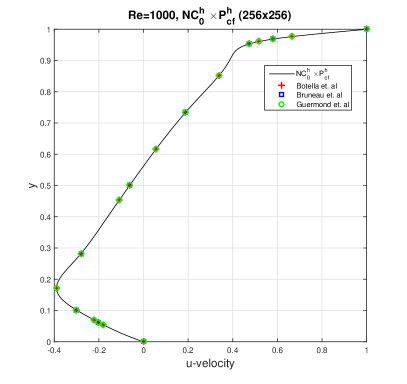
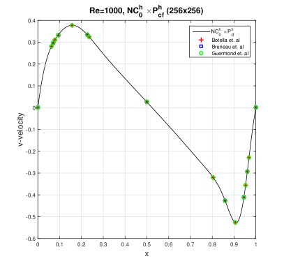
Figure 1: Comparison of the vertical components of the $u$-velocity along the segment $x\in[0,1]$, $y=1/2$ and the horizontal components of the $v$-velocity along the segment $x\in[0,1]$, $y=1/2$ with $Re=1000$

For the range of $Re=100,400,1000,2500,3200,$ and 5000, Figs. 2 and 3 show the $u$-velocity profiles along the line $x=0.5$ and the $v$-velocity profiles along the line $y=0.5$ computed by using the $\boldsymbol{\mathscr{P}}_{1,0}^{nc,h}\times\widetilde{{\mathscr{P}}_{0}^{h}}$ element with the boundary condition (3) and comparison results with those by Erturk et al. [18] and Ghia et al. [19]. In each case, our velocity profiles show a good agreement with their results.

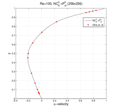
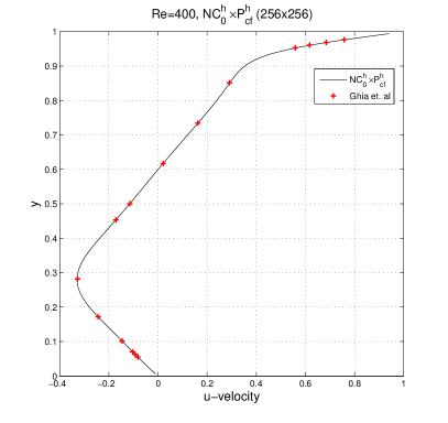
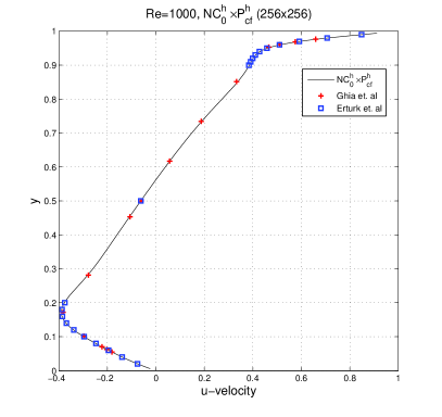
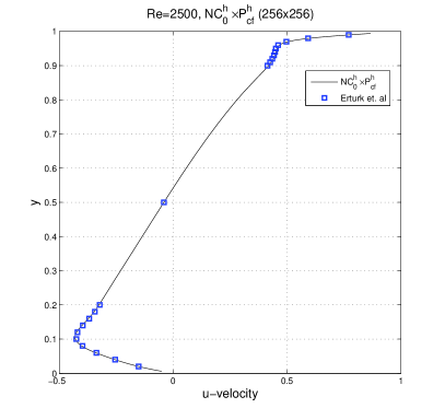
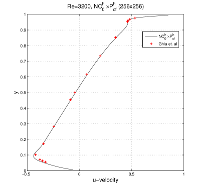
Figure 2: Profiles of $u$-velocity along the line $x=0.5$ computed by using the stable $\boldsymbol{\mathscr{P}}_{1,0}^{nc,h}\times\widetilde{{\mathscr{P}}_{0}^{h}}$ with unregularized boundary condition

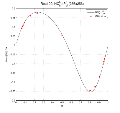
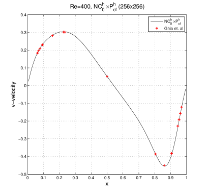
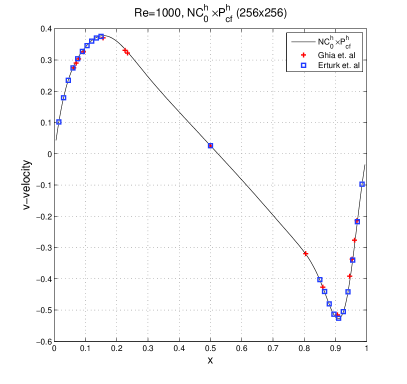
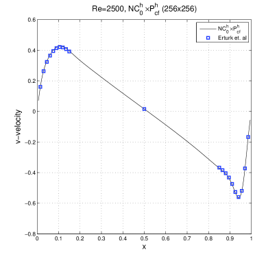
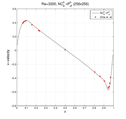
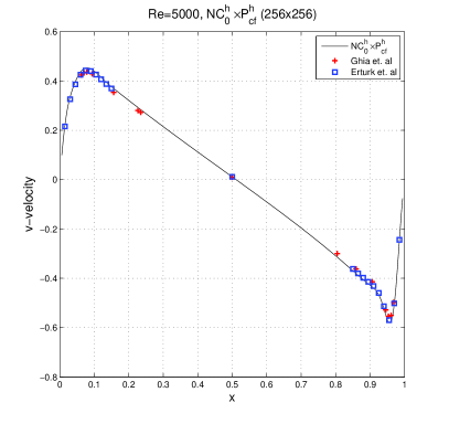
Figure 3: Profiles of $v$-velocity along the line $y=0.5$ computed by using the $\boldsymbol{\mathscr{P}}_{1,0}^{nc,h}\times\widetilde{{\mathscr{P}}_{0}^{h}}$ with unregularized boundary condition

Although the velocity profiles in Fig. 1 and Figs. 2 and 3 seem to match quite well for $Re=1000$, some of the actual numerical values differ in digits compared to those reported in [8, 9, 24]. Hence, we compare the numerical values of the horizontal and vertical components of the velocity in Tables 4 and 5 with the reference solutions from [8, 9, 24]. Our numerical values, which were computed with $256\times 256$ meshes with the lowest possible finite element $\boldsymbol{\mathscr{P}}_{1,0}^{nc,h}\times\widetilde{{\mathscr{P}}_{0}^{h}}$, match with the reference values mostly up to two digits, or with less than 1% errors; the numerical solutions, computed $512\times 512$ meshes match with the reference values mostly up to three digits, or with less than 0.1% errors.

Table 4: Comparison of the horizontal components of the velocity along the segment $y\in[0,1]$, $x=1/2$ at $Re=1000$

$y$	[8]	[9]	[24]	$\boldsymbol{\mathscr{P}}_{1,0}^{nc,h}\times\widetilde{{\mathscr{P}}_{0}^{h}}(256\times 256)$	$\boldsymbol{\mathscr{P}}_{1,0}^{nc,h}\times\widetilde{{\mathscr{P}}_{0}^{h}}(512\times 512)$
0.0000	0.0000000	0.00000	0.0000000	0.0000000	0.0000000
0.0312	-0.2279225	NA	-0.2279177	-0.2274204	-0.2276650
0.0391	-0.2936869	-0.29330	-0.2936814	-0.2930076	-0.2933552
0.0469	-0.3553213	NA	-0.3553154	-0.3545665	-0.3549485
0.0547	-0.4103754	-0.41018	-0.4103691	-0.4096654	-0.4100002
0.0937	-0.5264392	NA	-0.5264320	-0.5271749	-0.5264518
0.1406	-0.4264545	-0.42645	-0.4264492	-0.4276315	-0.4265356
0.1953	-0.3202137	NA	-0.3202068	-0.3209943	-0.3200577
0.5000	0.0257995	0.02580	0.0257987	0.0256839	0.0257175
0.7656	0.3253592	NA	0.3253529	0.3259697	0.3252217
0.7734	0.3339924	0.33398	0.3339860	0.3346373	0.3338694
0.8437	0.3769189	NA	0.3769119	0.3778450	0.3769140
0.9062	0.3330442	0.33290	0.3330381	0.3339829	0.3331021
0.9219	0.3099097	NA	0.3099041	0.3108006	0.3099725
0.9297	0.2962703	0.29622	0.2962650	0.2971221	0.2963312
0.9375	0.2807056	NA	0.2807005	0.2815029	0.2807605
1.0000	0.0000000	0.00000	0.0000000	0.0000000	0.0000000

Table 5: Comparison of the vertical components of the velocity along the segment $x\in[0,1]$, $y=1/2$ at $Re=1000$

$x$	[8]	[9]	[24]	$\boldsymbol{\mathscr{P}}_{1,0}^{nc,h}\times\widetilde{{\mathscr{P}}_{0}^{h}}(256\times 256)$	$\boldsymbol{\mathscr{P}}_{1,0}^{nc,h}\times\widetilde{{\mathscr{P}}_{0}^{h}}(512\times 512)$
1.0000	-1.0000000	-1.00000	-1.0000000	-1.0000000	-1.0000000
0.9766	-0.6644227	NA	-0.6644194	-0.6666343	-0.6648562
0.9688	-0.5808359	-0.58031	-0.5808318	-0.5831751	-0.5812660
0.9609	-0.5169277	NA	-0.5169214	-0.5190905	-0.5172781
0.9531	-0.4723329	-0.47239	-0.4723260	-0.4741970	-0.4725743
0.8516	-0.3372212	NA	-0.3372128	-0.3380993	-0.3370508
0.7344	-0.1886747	-0.18861	-0.1886680	-0.1890994	-0.1884232
0.6172	-0.0570178	NA	-0.0570151	-0.0570951	-0.0569011
0.5000	0.0620561	0.06205	0.0620535	0.0622962	-0.0619466
0.4531	0.1081999	NA	0.1081955	0.1085611	0.1080176
0.2813	0.2803696	0.28040	0.2803632	0.2811184	0.2802013
0.1719	0.3885691	NA	0.3885624	0.3894565	0.3885914
0.1016	0.3004561	0.30029	0.3004504	0.3006758	0.3004357
0.0703	0.2228955	NA	0.2228928	0.2228075	0.2228534
0.0625	0.2023300	0.20227	0.2023277	0.2021815	0.2022834
0.0547	0.1812881	NA	0.1812863	0.1810885	0.1812376
0.0000	0.0000000	0.00000	0.0000000	0.0000000	0.0000000

The computed streamlines are presented in Fig. 4. One can observe count-rotating secondary vortices at the bottom left and right corners of the square cavity. Bottom left and right vortices grow in size as Reynolds number increases and the secondary vortex at the top left corner of the square cavity develops as Reynolds number increases.

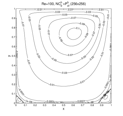
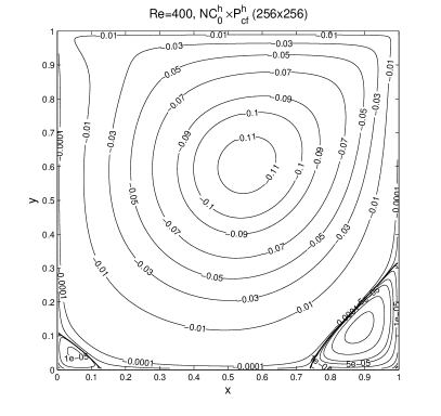
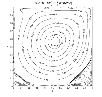
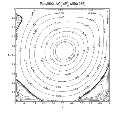
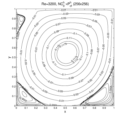
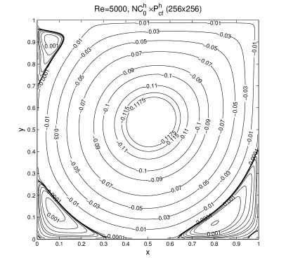
Figure 4: Streamline computed by using the $\boldsymbol{\mathscr{P}}_{1,0}^{nc,h}\times\widetilde{{\mathscr{P}}_{0}^{h}}$ element.

The vorticity contours are presented in Fig. 5. We observe that the gradient in vorticity is negligible in the center of cavity and the region of very low gradient in vorticity grows as Reynolds number increases.

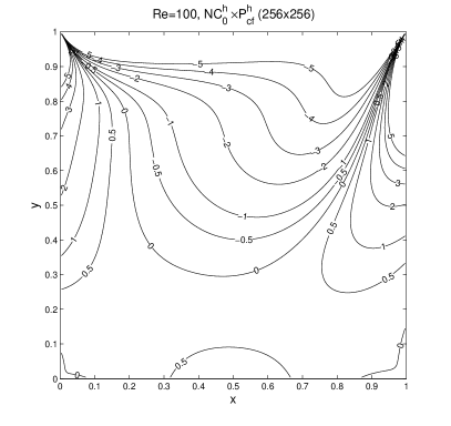
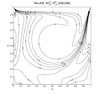
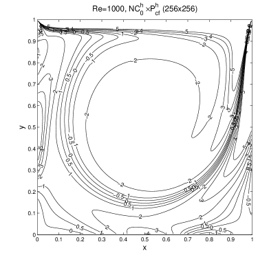
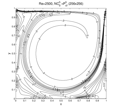
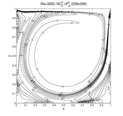
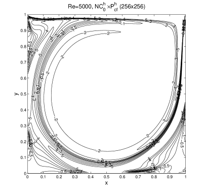
Figure 5: Contours of vorticity computed by using the $\boldsymbol{\mathscr{P}}_{1,0}^{nc,h}\times\widetilde{{\mathscr{P}}_{0}^{h}}$ element.

In Table 6, we present the location of the center of the primary vortex, the stream function $\psi$, and vorticity $\omega$ at vortex center. These data are calculated for $100\leq\text{Re}\leq 5000$; for comparison, available data from the literatures are also given. The values of the stream function $\psi$ and vorticity $\omega$ are recorded at the center of meshes. The locations of primary vortices computed by using the $\boldsymbol{\mathscr{P}}_{1,0}^{nc,h}\times\widetilde{{\mathscr{P}}_{0}^{h}}$ element differ from the other results by about $0.002$ which is half the mesh size $1/h\approx 0.0039$, Our numerical solutions computed by using both $\boldsymbol{\mathscr{P}}_{1,0}^{nc,h}\times\widetilde{{\mathscr{P}}_{0}^{h}}$ and $\boldsymbol{\mathscr{Q}}_{2,0}^{c,h}\times{\mathscr{Q}}_{1,0}^{dc,h}$ elements exhibit a good agreement with the literature data except in the case of the $\boldsymbol{\mathscr{Q}}_{2,0}^{c,h}\times{\mathscr{Q}}_{1,0}^{dc,h}$ element with leaky cavity boundary condition (25) applied. $\psi$ and $\omega$ for the $\boldsymbol{\mathscr{P}}_{1,0}^{nc,h}\times\widetilde{{\mathscr{P}}_{0}^{h}}$ element with (3) are similar to those in the literature [18, 19, 20, 32]. In addition, Table 7 summarizes data on the strengths and the locations of secondary vortices in the bottom left and right corners, and in the top left corner. We observe that secondary vortices appear stronger as the Reynolds number increases.

Table 6: Computed primary vortex; the values of stream function ($\psi$), vorticity ($\omega$), and location $(x,y)$.

Re	FEM	Grid	$\psi_{\min}$	$\omega$	$(x,y)$	BC
	$\boldsymbol{\mathscr{P}}_{1,0}^{nc,h}\times\widetilde{{\mathscr{P}}_{0}^{h}}$	$256\times 256$	-0.103531	3.16206	(0.6152,0.7363)	(3)
	$\boldsymbol{\mathscr{Q}}_{2,0}^{c,h}\times{\mathscr{Q}}_{1,0}^{dc,h}$	$128\times 128$	-0.103519	3.18101	(0.6172,0.7383)	(24)
	$\boldsymbol{\mathscr{Q}}_{2,0}^{c,h}\times{\mathscr{Q}}_{1,0}^{dc,h}$	$128\times 128$	-0.102872	3.15485	(0.6172,0.7383)	(25)
100	[19]	$129\times 129$	-0.103423	3.16646	(0.6172,0.7344)	-
	[20]	$128\times 128$	-0.103435	-	(0.6172,0.7344)	[20]
	[32]	$257\times 257$	-0.103471	3.1655	(0.6189,0.7400)	[32]
	$\boldsymbol{\mathscr{P}}_{1,0}^{nc,h}\times\widetilde{{\mathscr{P}}_{0}^{h}}$	$256\times 256$	-0.114071	2.29821	(0.5527,0.6035)	(3)
	$\boldsymbol{\mathscr{Q}}_{2,0}^{c,h}\times{\mathscr{Q}}_{1,0}^{dc,h}$	$128\times 128$	-0.113990	2.29476	(0.5547,0.6055)	(24)
	$\boldsymbol{\mathscr{Q}}_{2,0}^{c,h}\times{\mathscr{Q}}_{1,0}^{dc,h}$	$128\times 128$	-0.111900	2.26041	(0.5547,0.6055)	(25)
400	[19]	$257\times 257$	-0.113909	2.29469	(0.5547,0.6055)	-
	[20]	$128\times 128$	-0.113909	-	(0.5547,0.6094)	[20]
	[32]	$257\times 257$	-0.113897	2.2950	(0.5536,0.6075)	[32]
	$\boldsymbol{\mathscr{P}}_{1,0}^{nc,h}\times\widetilde{{\mathscr{P}}_{0}^{h}}$	$256\times 256$	-0.119186	2.07216	(0.5293,0.5645)	(3)
	$\boldsymbol{\mathscr{Q}}_{2,0}^{c,h}\times{\mathscr{Q}}_{1,0}^{dc,h}$	$128\times 128$	-0.118941	2.06779	(0.5313,0.5664)	(24)
	$\boldsymbol{\mathscr{Q}}_{2,0}^{c,h}\times{\mathscr{Q}}_{1,0}^{dc,h}$	$128\times 128$	-0.115376	2.00941	(0.5313,0.5664)	(25)
1000	[18]	$601\times 601$	-0.118781	2.06553	(0.5300,0.5650)	-
	[19]	$257\times 257$	-0.117929	2.04968	(0.5313,0.5625)	-
	[20]	$128\times 128$	-0.119173	-	(0.5313,0.5625)	[20]
	[32]	$257\times 257$	-0.118800	2.0664	(0.5335,0.5639)	[32]
	$\boldsymbol{\mathscr{P}}_{1,0}^{nc,h}\times\widetilde{{\mathscr{P}}_{0}^{h}}$	$256\times 256$	-0.122151	1.98912	(0.5215,0.5449)	(3)
	$\boldsymbol{\mathscr{Q}}_{2,0}^{c,h}\times{\mathscr{Q}}_{1,0}^{dc,h}$	$128\times 128$	-0.121492	1.97645	(0.5195,0.5430)	(24)
2500	$\boldsymbol{\mathscr{Q}}_{2,0}^{c,h}\times{\mathscr{Q}}_{1,0}^{dc,h}$	$128\times 128$	-0.115717	1.88476	(0.5195,0.5430)	(25)
	[18]	$601\times 601$	-0.121035	1.96968	(0.5200,0.5433)	-
	$\boldsymbol{\mathscr{P}}_{1,0}^{nc,h}\times\widetilde{{\mathscr{P}}_{0}^{h}}$	$256\times 256$	-0.122713	1.97778	(0.5176,0.5410)	(3)
	$\boldsymbol{\mathscr{Q}}_{2,0}^{c,h}\times{\mathscr{Q}}_{1,0}^{dc,h}$	$128\times 128$	-0.121860	1.96186	(0.5195,0.5391)	(24)
	$\boldsymbol{\mathscr{Q}}_{2,0}^{c,h}\times{\mathscr{Q}}_{1,0}^{dc,h}$	$128\times 128$	-0.115310	1.85833	(0.5195,0.5430)	(25)
3200	[19]	$257\times 257$	-0.120377	1.98860	(0.5165,0.5469)	-
	[20]	$128\times 128$	-0.121768	-	(0.5165,0.5352)	[20]
	[32]	$257\times 257$	-0.121628	1.9593	(0.5201,0.5376)	[32]
	$\boldsymbol{\mathscr{P}}_{1,0}^{nc,h}\times\widetilde{{\mathscr{P}}_{0}^{h}}$	$256\times 256$	-0.123658	1.96650	(0.5137,0.5371)	(3)
	$\boldsymbol{\mathscr{Q}}_{2,0}^{c,h}\times{\mathscr{Q}}_{1,0}^{dc,h}$	$128\times 128$	-0.122368	1.94277	(0.5156,0.5352)	(24)
	$\boldsymbol{\mathscr{Q}}_{2,0}^{c,h}\times{\mathscr{Q}}_{1,0}^{dc,h}$	$128\times 128$	-0.114120	1.81321	(0.5156,0.5352)	(25)
5000	[18]	$601\times 601$	-0.121289	1.92660	(0.5150,0.5350)	-
	[19]	$257\times 257$	-0.118966	1.86016	(0.5117,0.5352)	-
	[20]	$128\times 128$	-0.121218	-	(0.5156,0.5352)	[20]
	[32]	$257\times 257$	-0.122050	1.9392	(0.5134,0.5376)	[32]

Table 7: Computed secondary vortices; the values of stream function ($\psi$) and location $(x,y)$ for the $\boldsymbol{\mathscr{P}}_{1,0}^{nc,h}\times\widetilde{{\mathscr{P}}_{0}^{h}}$ element.

	Bottom left		Bottom Right		Top left
Re	$\psi_{\max}$	$(x,y)$	$\psi_{\max}$	$(x,y)$	$\psi_{\max}$	$(x,y)$
100	1.7368E-06	(0.0332,0.0332)	1.2597E-05	(0.9434,0.0605)	-	-
400	1.4100E-05	(0.0488,0.0488)	6.4495E-04	(0.8848,0.1230)	-	-
1000	2.3223E-04	(0.0840,0.0762)	1.7319E-03	(0.8652,0.1113)	-	-
2500	9.2779E-04	(0.0840,0.1113)	2.6661E-03	(0.8340,0.0918)	3.3918E-04	(0.0410,0.8887)
3200	1.1104E-03	(0.0801,0.1191)	2.8323E-03	(0.8223,0.0840)	7.0750E-04	(0.0527,0.8965)
5000	1.3660E-03	(0.0723,0.1387)	3.0641E-03	(0.8027,0.0723)	1.4566e-03	(0.0645,0.9082)

In §4, we introduced the indicators for the accuracy of the numerical solution. First, the volumetric flow rate values $Q_{u,x_{c}}$ and $Q_{v,y_{c}}$ defined by (10) are shown in Table 8. for the $\boldsymbol{\mathscr{P}}_{1,0}^{nc,h}\times\widetilde{{\mathscr{P}}_{0}^{h}}$ element The values of $Q_{u,x_{c}}$ and $Q_{v,y_{c}}$ for the $\boldsymbol{\mathscr{Q}}_{2,0}^{c,h}\times{\mathscr{Q}}_{1,0}^{dc,h}$ element are much larger than those values at $Q_{u,x_{c}-h/2}$, $Q_{u,x_{c}+h/2}$, $Q_{v,y_{c}-h/2}$, and $Q_{v,y_{c}+h/2}$ for the $\boldsymbol{\mathscr{P}}_{1,0}^{nc,h}\times\widetilde{{\mathscr{P}}_{0}^{h}}$ element. Erturk et al. [18] calculated $Q_{u,x_{c}}$and $Q_{v,y_{c}}$ by using their solutions. The smallest values of $Q_{u,x_{c}}=4.5\text{E-8}$ and $Q_{v,y_{c}}=1.34\text{E-7}$ in [18] are lager than the largest values of $Q_{u}$ and $Q_{v}$ for the $\boldsymbol{\mathscr{P}}_{1,0}^{nc,h}\times\widetilde{{\mathscr{P}}_{0}^{h}}$ element.

Table 9 shows the values of (12) and (13) for the $\boldsymbol{\mathscr{P}}_{1,0}^{nc,h}\times\widetilde{{\mathscr{P}}_{0}^{h}}$ and the $\boldsymbol{\mathscr{Q}}_{2,0}^{c,h}\times{\mathscr{Q}}_{1,0}^{dc,h}$ elements. Concerning the compatibility condition (12), the $\boldsymbol{\mathscr{P}}_{1,0}^{nc,h}\times\widetilde{{\mathscr{P}}_{0}^{h}}$ element and the Taylor-Hood element with the leaky cavity boundary condition (25) give precise values, while the Taylor-Hood element with the watertight cavity boundary condition (24) generates about 0.3% errors. An investigation of (13) shows that the numerical results obtained by using the $\boldsymbol{\mathscr{P}}_{1,0}^{nc,h}\times\widetilde{{\mathscr{P}}_{0}^{h}}$ element are more accurate than those by the Taylor-Hood element. Moreover, the absolute values (13) for the $\boldsymbol{\mathscr{P}}_{1,0}^{nc,h}\times\widetilde{{\mathscr{P}}_{0}^{h}}$ element are independent of Reynolds number and element $Q_{jk}$ due to Theorem 4.1. With the grid size $256\times 256$, the absolute values (13) for the $\boldsymbol{\mathscr{P}}_{1,0}^{nc,h}\times\widetilde{{\mathscr{P}}_{0}^{h}}$ element is given by

$$\max_{Q_{jk}\in\mathscr{T}_{h}}\left|\int_{Q_{jk}}\nabla\cdot\,\mathbf{u}_{h}\operatorname{\,d\mathbf{x}}\right|=\frac{1}{256^{3}}\approx 5.9605\text{E-8},$$ (26)

while such values for the Taylor-Hood element with watertight and leaky cavity boundary conditions are given in Table 9. It should be stressed that the values obtained by the $\boldsymbol{\mathscr{P}}_{1,0}^{nc,h}\times\widetilde{{\mathscr{P}}_{0}^{h}}$ element are smaller by a factor of four than those obtained by the Taylor-Hood element.

At least judged by the three accuracy indicators, (10), (12), and (13), the numerical solutions by using the $\boldsymbol{\mathscr{P}}_{1,0}^{nc,h}\times\widetilde{{\mathscr{P}}_{0}^{h}}$ element without any modification at the top corners are more accurate than those by using the Taylor-Hood element with modified boundary conditions (24) and (25).

Table 8: Volumetric flow rates along the vertical and horizontal lines through the geometric center of the cavity, $(x_{c},y_{c})$, by using the $\boldsymbol{\mathscr{P}}_{1,0}^{nc,h}\times\widetilde{{\mathscr{P}}_{0}^{h}}$ and $\boldsymbol{\mathscr{Q}}_{2,0}^{c,h}\times{\mathscr{Q}}_{1,0}^{dc,h}$ element

Re	FEM	Grid	$Q_{u,x_{c}}$	$Q_{v,y_{c}}$	BC
	$\boldsymbol{\mathscr{P}}_{1,0}^{nc,h}\times\widetilde{{\mathscr{P}}_{0}^{h}}$	$256\times 256$	1.9039e-16	1.2514e-13	(3)
100	$\boldsymbol{\mathscr{Q}}_{2,0}^{c,h}\times{\mathscr{Q}}_{1,0}^{dc,h}$	$128\times 128$	9.3009E-06	6.5662E-08	(24)
	$\boldsymbol{\mathscr{Q}}_{2,0}^{c,h}\times{\mathscr{Q}}_{1,0}^{dc,h}$	$128\times 128$	1.3114E-03	9.7804E-08	(25)
	$\boldsymbol{\mathscr{P}}_{1,0}^{nc,h}\times\widetilde{{\mathscr{P}}_{0}^{h}}$	$256\times 256$	2.1554e-16	1.3347e-13	(3)
400	$\boldsymbol{\mathscr{Q}}_{2,0}^{c,h}\times{\mathscr{Q}}_{1,0}^{dc,h}$	$128\times 128$	1.4876E-05	1.2495E-06	(24)
	$\boldsymbol{\mathscr{Q}}_{2,0}^{c,h}\times{\mathscr{Q}}_{1,0}^{dc,h}$	$128\times 128$	1.3170E-03	1.1132E-06	(25)
	$\boldsymbol{\mathscr{P}}_{1,0}^{nc,h}\times\widetilde{{\mathscr{P}}_{0}^{h}}$	$256\times 256$	3.5996e-17	1.1037e-14	(3)
1000	$\boldsymbol{\mathscr{Q}}_{2,0}^{c,h}\times{\mathscr{Q}}_{1,0}^{dc,h}$	$128\times 128$	2.4097E-05	2.8794E-06	(24)
	$\boldsymbol{\mathscr{Q}}_{2,0}^{c,h}\times{\mathscr{Q}}_{1,0}^{dc,h}$	$128\times 128$	1.3264E-03	2.5407E-06	(25)
	$\boldsymbol{\mathscr{P}}_{1,0}^{nc,h}\times\widetilde{{\mathscr{P}}_{0}^{h}}$	$256\times 256$	2.4373e-16	1.5280e-13	(3)
2500	$\boldsymbol{\mathscr{Q}}_{2,0}^{c,h}\times{\mathscr{Q}}_{1,0}^{dc,h}$	$128\times 128$	4.0694E-05	5.7553E-06	(24)
	$\boldsymbol{\mathscr{Q}}_{2,0}^{c,h}\times{\mathscr{Q}}_{1,0}^{dc,h}$	$128\times 128$	1.3431E-03	4.8544E-06	(25)
	$\boldsymbol{\mathscr{P}}_{1,0}^{nc,h}\times\widetilde{{\mathscr{P}}_{0}^{h}}$	$256\times 256$	2.1814e-16	5.1092e-14	(3)
3200	$\boldsymbol{\mathscr{Q}}_{2,0}^{c,h}\times{\mathscr{Q}}_{1,0}^{dc,h}$	$128\times 128$	4.6986E-05	7.0223E-06	(24)
	$\boldsymbol{\mathscr{Q}}_{2,0}^{c,h}\times{\mathscr{Q}}_{1,0}^{dc,h}$	$128\times 128$	1.3494E-03	5.8405E-06	(25)
	$\boldsymbol{\mathscr{P}}_{1,0}^{nc,h}\times\widetilde{{\mathscr{P}}_{0}^{h}}$	$256\times 256$	3.5562e-16	1.2311e-13	(3)
5000	$\boldsymbol{\mathscr{Q}}_{2,0}^{c,h}\times{\mathscr{Q}}_{1,0}^{dc,h}$	$128\times 128$	6.1055E-05	1.0206E-05	(24)
	$\boldsymbol{\mathscr{Q}}_{2,0}^{c,h}\times{\mathscr{Q}}_{1,0}^{dc,h}$	$128\times 128$	1.3634E-03	8.2691E-06	(25)

Table 9: Compatibility (12) and incompressibility conditions (13) for the $\boldsymbol{\mathscr{P}}_{1,0}^{nc,h}\times\widetilde{{\mathscr{P}}_{0}^{h}}$ and $\boldsymbol{\mathscr{Q}}_{2,0}^{c,h}\times{\mathscr{Q}}_{1,0}^{dc,h}$ elements.

Re	FEM	Grid	$|\int_{\Omega}\omega\;\operatorname{\,d\mathbf{x}}+1|$	(13)	BC
	$\boldsymbol{\mathscr{P}}_{1,0}^{nc,h}\times\widetilde{{\mathscr{P}}_{0}^{h}}$	$256\times 256$	2.8866e-15	5.9605E-08	(3)
100	$\boldsymbol{\mathscr{Q}}_{2,0}^{c,h}\times{\mathscr{Q}}_{1,0}^{dc,h}$	$128\times 128$	2.6042e-03	6.1596E-04	(24)
	$\boldsymbol{\mathscr{Q}}_{2,0}^{c,h}\times{\mathscr{Q}}_{1,0}^{dc,h}$	$128\times 128$	1.1102e-15	3.3407E-04	(25)
	$\boldsymbol{\mathscr{P}}_{1,0}^{nc,h}\times\widetilde{{\mathscr{P}}_{0}^{h}}$	$256\times 256$	2.2204e-16	5.9605E-08	(3)
400	$\boldsymbol{\mathscr{Q}}_{2,0}^{c,h}\times{\mathscr{Q}}_{1,0}^{dc,h}$	$128\times 128$	2.6042e-03	6.6730E-04	(24)
	$\boldsymbol{\mathscr{Q}}_{2,0}^{c,h}\times{\mathscr{Q}}_{1,0}^{dc,h}$	$128\times 128$	4.7740e-15	3.9730E-04	(25)
	$\boldsymbol{\mathscr{P}}_{1,0}^{nc,h}\times\widetilde{{\mathscr{P}}_{0}^{h}}$	$256\times 256$	2.6645e-15	5.9605E-08	(3)
1000	$\boldsymbol{\mathscr{Q}}_{2,0}^{c,h}\times{\mathscr{Q}}_{1,0}^{dc,h}$	$128\times 128$	2.6042e-03	7.2274E-04	(24)
	$\boldsymbol{\mathscr{Q}}_{2,0}^{c,h}\times{\mathscr{Q}}_{1,0}^{dc,h}$	$128\times 128$	1.5543e-15	5.0746E-04	(25)
	$\boldsymbol{\mathscr{P}}_{1,0}^{nc,h}\times\widetilde{{\mathscr{P}}_{0}^{h}}$	$256\times 256$	1.1102e-15	5.9605E-08	(3)
2500	$\boldsymbol{\mathscr{Q}}_{2,0}^{c,h}\times{\mathscr{Q}}_{1,0}^{dc,h}$	$128\times 128$	2.6042e-03	1.1836E-03	(24)
	$\boldsymbol{\mathscr{Q}}_{2,0}^{c,h}\times{\mathscr{Q}}_{1,0}^{dc,h}$	$128\times 128$	7.7716e-15	5.9441E-04	(25)
	$\boldsymbol{\mathscr{P}}_{1,0}^{nc,h}\times\widetilde{{\mathscr{P}}_{0}^{h}}$	$256\times 256$	3.9968e-15	5.9605E-08	(3)
3200	$\boldsymbol{\mathscr{Q}}_{2,0}^{c,h}\times{\mathscr{Q}}_{1,0}^{dc,h}$	$128\times 128$	2.6042e-03	1.3685E-03	(24)
	$\boldsymbol{\mathscr{Q}}_{2,0}^{c,h}\times{\mathscr{Q}}_{1,0}^{dc,h}$	$128\times 128$	1.5543e-15	6.0657E-04	(25)
	$\boldsymbol{\mathscr{P}}_{1,0}^{nc,h}\times\widetilde{{\mathscr{P}}_{0}^{h}}$	$256\times 256$	1.4433e-15	5.9605E-08	(3)
5000	$\boldsymbol{\mathscr{Q}}_{2,0}^{c,h}\times{\mathscr{Q}}_{1,0}^{dc,h}$	$128\times 128$	2.6042e-03	1.6240E-03	(24)
	$\boldsymbol{\mathscr{Q}}_{2,0}^{c,h}\times{\mathscr{Q}}_{1,0}^{dc,h}$	$128\times 128$	4.2188e-15	6.7909E-04	(25)

6 Conclusions

The $\boldsymbol{\mathscr{P}}_{1,0}^{nc,h}\times\widetilde{{\mathscr{P}}_{0}^{h}}$ element is applied to solve the lid driven cavity problem with least modification at the two top corner element to deal with the jump discontinuities there using the DSSY element (of CDY element).

The numerical solutions using $\boldsymbol{\mathscr{P}}_{1,0}^{nc,h}\times\widetilde{{\mathscr{P}}_{0}^{h}}$ element are compared with bench mark solutions and the horizontal and vertical components of the velocity at the center are correct up to mostly two and three digits if the mesh sizes are $256\times 256$ and $512\times 512,$ respectively.

Numerical solutions were compared with those the conforming $\boldsymbol{\mathscr{Q}}_{2,0}^{c,h}\times{\mathscr{Q}}_{1,0}^{dc,h}$ element (Taylor-Hood element) with leaky and watertight cavity boundary conditions. Three indicators for accuracy of the numerical solution have been compared. (1) The incompressibility condition (2) The compatibility condition (3) with the Neumann boundary condition are used to check the accuracy of the numerical solutions.

Our numerical solutions satisfy the incompressibility and compatibility condition precisely. Numerical results computed by using the $\boldsymbol{\mathscr{P}}_{1,0}^{nc,h}\times\widetilde{{\mathscr{P}}_{0}^{h}}$ element show the best results in terms of satisfying incompressibility and compatibility conditions, and volumetric flow rates.

References

- [1] Incompressible Flow & Iterative Solver Software. http://www.maths.manchester.ac.uk/ djs/ifiss.
- [2] R. Altmann and C. Carstensen. -nonconforming finite elements on triangulations into triangles and quadrilaterals. SIAM J. Numer. Anal., 50(2):418–438, 2011.
- [3] R. Altmann and C. Carstensen. -nonconforming finite elements on triangulations into triangles and quadrilaterals. SIAM Journal on Numerical Analysis, 50(2):418–438, 2012.
- [4] F. Auteri, N. Parolini, and L. Quartapelle. Numerical investigation on the stability of singular driven cavity flow. Journal of Computational Physics, 183(1):1–25, 2002.
- [5] M. Aydin and R. Fenner. Boundary element analysis of driven cavity flow for low and moderate Reynolds number. Int. J. Numer. Meth. Fluids., 37:45–64, 2001.
- [6] E. Barragy and G. Carey. Stream function-vorticity driven cavity solution using finite elements. Computers & Fluids, 26:453–468, 1997.
- [7] M. Bercovier and O. Pironneau. Error estimates for finite element method solution of the Stokes problem in the primitive variables. Numer. Math., 33(2):211–224, 1979.
- [8] O. Botella and R. Peyret. Benchmark spectral results on the lid-driven cavity flow. Computers & Fluids, 27(4):421–433, 1998.
- [9] C.-H. Bruneau and M. Saad. The 2D lid–driven cavity problem revisited. Computers & Fluids, 35(3):326–348, 2006.
- [10] Z. Cai, J. Douglas, Jr., J. E. Santos, D. Sheen, and X. Ye. Nonconforming quadrilateral finite elements: A correction. Calcolo, 37(4):253–254, 2000.
- [11] Z. Cai, J. Douglas, Jr., and X. Ye. A stable nonconforming quadrilateral finite element method for the stationary Stokes and Navier-Stokes equations. Calcolo, 36:215–232, 1999.
- [12] Z. Cai and Y. Wang. An error estimate for two-dimensional Stokes driven cavity flow. Math. Comp., 78:771–787, 2008.
- [13] M. Crouzeix and P.-A. Raviart. Conforming and nonconforming finite element methods for solving the stationary Stokes equations. R.A.I.R.O.– Math. Model. Anal. Numer., 7:33–75, 1973.
- [14] C. Cuvelier, A. Segal, and A. A. Van Steenhoven. Finite element methods and Navier–Stokes equations, volume 22. Springer, 1986.
- [15] J. Douglas, Jr., J. E. Santos, D. Sheen, and X. Ye. Nonconforming Galerkin methods based on quadrilateral elements for second order elliptic problems. ESAIM–Math. Model. Numer. Anal., 33(4):747–770, 1999.
- [16] H. Elman, D. Silvester, and A. Wathen. Finite elements and fast iterative solvers: with applications in incompressible fluid dynamics. Oxford University Press, 2014.
- [17] E. Erturk. Discussions on driven cavity flow. International Journal for Numerical Methods in Fluids, 60(3):275–294, 2009.
- [18] E. Erturk, T. C. Corke, and C. Gökçöl. Numerical solutions of 2-D steady incompressible driven cavity flow at high Reynolds numbers. International Journal for Numerical Methods in Fluids, 48(7):747–774, 2005.
- [19] U. Ghia, K. N. Ghia, and C. T. Shin. High-Re solutions for incompressible flow using the Navier-Stokes equations and a multigrid method. J. Comp. Phys., 48:387–411, 1982.
- [20] R. Glowinski. Finite element methods for incompressible viscous flow. In P. G. Ciarlet and J. L. Lions, editors, Handbook of Numerical Analysis. IX. Numerical Methods for Fluids (Part 3). Elsevier/North-Holland, Amsterdam, 2003.
- [21] R. Glowinski, G. Guidoboni, and T.-W. Pan. Wall-driven incompressible viscous flow in a two-dimensional semi-circular cavity. J. Comp. Phys., 216(1):76–91, 2006.
- [22] J.-L. Guermond and P. Minev. A new class of massively parallel direction splitting for the incompressible Navier–Stokes equations. Computer Methods in Applied Mechanics and Engineering, 200(23):2083–2093, 2011.
- [23] J.-L. Guermond and P. D. Minev. A new class of fractional step techniques for the incompressible Navier–Stokes equations using direction splitting. Comptes Rendus Mathematique, 348(9):581–585, 2010.
- [24] J.-L. Guermond and P. D. Minev. Start-up flow in a three-dimensional lid-driven cavity by means of a massively parallel direction splitting algorithm. International Journal for Numerical Methods in Fluids, 68(7):856–871, 2012.
- [25] P. Hood and C. Taylor. A numerical solution of the Navier–Stokes equations using the finite element techniques. Computers & Fluids, 1:73–100, 1973.
- [26] Y. Jeon, H. Nam, D. Sheen, and K. Shim. A class of nonparametric DSSY nonconforming quadrilateral elements. ESAIM–Math. Model. Numer. Anal., 47(06):1783–1796, 2013.
- [27] O. A. Karakashian. On a Galerkin–Lagrange multiplier method for the stationary Navier–Stokes equations. SIAM J. Numer. Anal., 19(5):909–923, 1982.
- [28] S. Kim, J. Yim, and D. Sheen. Stable cheapest nonconforming finite elements for the Stokes equations. J. Comput. Appl. Math., 299:2-14, 2016.
- [29] C. Park. A study on locking phenomena in finite element methods. PhD thesis, Department of Mathematics, Seoul National University, Korea, Feb. 2002. Available at http://www.nasc.snu.ac.kr/cpark/papers/phdthesis.ps.gz.
- [30] C. Park and D. Sheen. -nonconforming quadrilateral finite element methods for second-order elliptic problems. SIAM J. Numer. Anal., 41(2):624–640, 2003.
- [31] R. Rannacher and S. Turek. Simple nonconforming quadrilateral Stokes element. Numer. Methods Partial Differential Equations, 8:97–111, 1992.
- [32] M. Sahin and R. Owens. A novel fully implicit finite volume methods applied to the lid-driven cavity problem–Part I: High Reynolds number flow calculations. Int. J. Numer. Meth. Fluids., 42:57–77, 2003.
- [33] J. Shen. Hopf bifurcation of the unsteady regularized driven cavity flow. J. Comp. Phys., 95:228–245, 1991.