A phenomenological analysis of azimuthal asymmetries
in unpolarized semi-inclusive deep inelastic scattering

Abstract

We present a phenomenological analysis of the $\cos\phi$ and $\cos 2\phi$ asymmetries in unpolarized semi-inclusive deep inelastic scattering, based on the recent multidimensional data released by the COMPASS and HERMES Collaborations. In the TMD framework, valid at relatively low transverse momenta, these asymmetries arise from intrinsic transverse momentum and transverse spin effects, and from their correlations. The role of the Cahn and Boer–Mulders effects in both azimuthal moments is explored up to order $1/Q$. As the kinematics of the present experiments is dominated by the low-$Q^{2}$ region, higher-twist contributions turn out to be important, affecting the results of our fits.

I Introduction

Since the early QCD investigations of hadronic hard processes, it has been recognized that azimuthal asymmetries in unpolarized reactions, such as Drell-Yan production and semi-inclusive deep inelastic scattering (SIDIS), represent an important window on the perturbative and non-perturbative aspects of strong interactions Georgi:1977tv ; Mendez:1978zx . Focusing on SIDIS processes, while at large momentum transfer $Q$ and large $P_{T}$ (the transverse momentum of the produced hadron), the azimuthal asymmetries are perturbatively generated by gluon radiation, at small $P_{T}$, $P_{T}\ll Q$, they can arise from the intrinsic motion of quarks Cahn:1978se ; Cahn:1989yf ; Konig:1982uk ; Chay:1991nh (for a review, see Ref. Barone:2010zz ). In the latter regime, the so-called transverse-momentum-dependent (TMD) factorization applies, and the SIDIS structure functions (in the current fragmentation region) can be written as transverse-momentum convolutions of TMD distribution and fragmentation functions Ji:2004wu .

Two azimuthal modulations appear in the unpolarized SIDIS cross section, of the type $\cos\phi$ and $\cos 2\phi$, where $\phi$ is the azimuthal angle of the produced hadron (measured from the scattering plane). These asymmetries, which have been experimentally investigated for the first time in the large $Q^{2}$ region by the EMC and ZEUS experiments Aubert:1983cz ; Arneodo:1986cf ; Breitweg:2000qh , have recently attracted a large experimental and theoretical attention as a potential source of information, in the small $P_{T}$ region, on the so-called Boer–Mulders distribution function, $h_{1}^{\perp}$, which measures the transverse polarization asymmetry of quarks inside an unpolarized nucleon Boer:1997nt .

A few years ago the azimuthal asymmetries in unpolarized SIDIS have been measured by the COMPASS and HERMES Collaborations for positive and negative hadrons, and presented as one-dimensional projections, with all variables $(x_{B},z_{h},Q^{2},P_{T})$ but one integrated over Kafer:2008ud ; Bressan:2009eu ; Giordano:2009hi .

The one-dimensional data on the $\cos 2\phi$ asymmetry were analyzed in Ref. Barone:2009hw , where it was shown that the larger asymmetry for $\pi^{-}(h^{-})$ production, compared to $\pi^{+}(h^{+})$, was an indication of the existence of a non-zero Boer–Mulders effect, in agreement with the earlier predictions of Ref. Barone:2008tn . It was also pointed out that measurements at different values of $Q^{2}$ were essential, in order to disentangle higher-twist contributions from the twist-two Boer-Mulder term.

The HERMES and COMPASS Collaborations have recently provided multidimensional data in bins of $x_{B},z_{h},Q^{2}$ and $P_{T}$ for the multiplicities Airapetian:2012ki ; Adolph:2013stb and for the azimuthal asymmetries Airapetian:2012yg ; Adolph:2014pwc . In principle, multidimensional data should offer detailed information, essential to unravel the kinematical behaviour of these asymmetries: for instance, the $Q^{2}$ dependence is crucial to disentangle higher-twist effects. In this paper, we present a study of the SIDIS azimuthal moments $\langle\cos\phi\rangle\,$and $\langle\cos 2\phi\rangle\,$in order to understand the role of the Cahn effect and to extract the Boer–Mulders function. We will see that, due to the present kinematics which is still dominated by the low-$Q^{2}$ region, the higher-twist contributions are important and strongly affect the results of our fits.

II Formalism

The process we are interested in is unpolarized SIDIS:

$$l(\ell)\,+\,N(P)\,\rightarrow\,l^{\prime}(\ell^{\prime})\,+\,h(P_{h})\,+\,X(P_{X})\,.$$ (1)

The cross section of this process is expressed in terms of the invariants

$$x_{B}=\frac{Q^{2}}{2\,P\cdot q},\;\;\;y=\frac{P\cdot q}{P\cdot\ell},\;\;\;z_{h}=\frac{P\cdot P_{h}}{P\cdot q}\,,$$ (2)

where $q=\ell-\ell^{\prime}$ and $Q^{2}\equiv-q^{2}$.

Figure 1: Kinematical configuration and conventions for SIDIS processes. The initial and final lepton momenta define the $\hat{x}$-$\hat{z}$ plane.

The reference frame we adopt is the $\gamma^{*}$-$N$ center-of-mass frame, with the virtual photon moving in the positive $z$ direction (Fig. 1). We denote by $\mbox{\boldmath$P$}_{T}$ the transverse momentum of the produced hadron. The azimuthal angle of this hadron referred to the lepton scattering plane will be called $\phi$.

The unpolarized SIDIS differential cross section is

$$\frac{{\mathrm{d}}\sigma}{{\mathrm{d}}x_{B}{\mathrm{d}}y{\mathrm{d}}z_{h}{\mathrm{d}}P_{T}^{2}{\mathrm{d}}\phi} = \frac{\pi\alpha^{2}}{Q^{2}xy}\left\{(1+(1-y)^{2})F_{UU}+2(2-y)\sqrt{1-y}F_{UU}^{\cos\phi}\cos\phi\right.$$ (3)

$$+\left.2(1-y)F_{UU}^{\cos(2\phi)}\cos(2\phi)\right\},$$

where the structure functions $F_{UU},F_{UU}^{\cos\phi},F_{UU}^{\cos 2\phi}$ depend on $x_{B},z_{h},Q^{2},P_{T}^{2}$. $F_{UU}$ is the structure function which survives upon integration over $\phi$, while $F_{UU}^{\cos\phi}$ and $F_{UU}^{\cos 2\phi}$ are associated to the $\cos\phi$ and $\cos 2\phi$ modulations, respectively.

If $k$ is the momentum of the quark inside the proton, and $\mbox{\boldmath$k$}_{\perp}$ its transverse component with respect to the $\gamma^{*}N$ axis, in the kinematical region where $P_{T}\sim k_{\perp}\ll Q$, the transverse-momentum-dependent (TMD) factorization is known to hold at leading twist. The structure functions can be expressed in terms of TMD distribution and fragmentation functions, which depend on the light-cone momentum fractions

$$x=\frac{k^{+}}{P^{+}}\,,\;\;\;z=\frac{P_{h}^{-}}{\kappa^{-}},$$ (4)

where $\kappa$ is the momentum of the fragmenting quark. Although the TMD factorization has not been rigorously proven at order $1/Q$ (that is, at twist three), in the following we will assume it to hold, as usually done in most phenomenological analyses.

Introducing the transverse momentum $\mbox{\boldmath$p$}_{\perp}$ of the final hadron with respect to the direction of the fragmenting quark, up to order $k_{\perp}/Q$ one has $\mbox{\boldmath$p$}_{\perp}=-z\mbox{\boldmath$\kappa$}_{\perp}$ and the momentum conservation reads

$$\hbox{\boldmath$P$\unboldmath}_{T}=z\mbox{\boldmath$k$}_{\perp}+\mbox{\boldmath$p$}_{\perp}.$$ (5)

At the same order we can identify the light-cone momentum fractions with the invariants $x_{B}$ and $z_{h}$,

$$x=x_{B},\;\;\;\;z=z_{h}.$$ (6)

In the TMD factorization scheme the structure function $F_{UU}$ is given by

$$F_{UU}=\sum_{q}e_{q}^{2}x\int{\mathrm{d}}^{2}\hbox{\boldmath$k$\unboldmath}_{\perp}\,f_{q}(x,k_{\perp})D_{q}(z,p_{\perp}),$$ (7)

where $f_{q}(x,k_{\perp})$ and $D_{q}(z,p_{\perp})$ are the unpolarized TMD distribution and fragmentation function, respectively, for the flavor $q$ (the sum is intended to be both over quarks and antiquarks). Note that in Eq. (7) the transverse momentum conservation has been applied, so that $p_{\perp}=|\hbox{\boldmath$P$\unboldmath}_{T}-z\mbox{\boldmath$k$}_{\perp}|$. The $Q^{2}$ dependence of all functions is omitted for simplicity.

The structure function associated with the $\cos\phi$ modulation turns out to be an order $1/Q$, i.e. a twist-3, quantity. Neglecting the dynamical twist-3 contributions (the so-called “tilde” functions, which arise from quark-gluon correlations), $F_{UU}^{\cos\phi}$ can be written as the sum of two terms

$$F_{UU}^{\cos\phi}=\left.F_{UU}^{\cos\phi}\right|_{\rm Cahn}+\left.F_{UU}^{\cos\phi}\right|_{\rm BM},$$ (8)

with ($\mbox{\boldmath$h$}\equiv\mbox{\boldmath$P$}_{T}/|\mbox{\boldmath$P$}_{T}|$)

$$\left.F_{UU}^{\cos\phi}\right|_{\rm Cahn}=-2\sum_{q}e_{q}^{2}x\int{\mathrm{d}}^{2}\mbox{\boldmath$k$}_{\perp}\,\frac{(\mbox{\boldmath$k$}_{\perp}\cdot\mbox{\boldmath$h$})}{Q}f_{q}(x,k_{\perp})D_{q}(z,p_{\perp}),$$ (9)

$$\left.F_{UU}^{\cos\phi}\right|_{\rm BM}=\sum_{q}e_{q}^{2}x\int{\mathrm{d}}^{2}\mbox{\boldmath$k$}_{\perp}\,\frac{k_{\perp}}{Q}\frac{P_{T}-z(\mbox{\boldmath$k$}_{\perp}\cdot\mbox{\boldmath$h$})}{k_{\perp}}\Delta f_{q^{\uparrow}/p}(x,k_{\perp})\Delta D_{h/q^{\uparrow}}(z,p_{\perp}).$$ (10)

Eq. (9) is the Cahn term, which accounts for the non-collinear kinematics of quarks in the elementary subprocess $\ell q\to\ell^{\prime}q^{\prime}$. Eq. (10) is the Boer–Mulders contribution, arising from the correlation between the transverse spin and the transverse momentum of quarks inside the unpolarized proton. In this term the Boer–Mulders distribution function $\Delta f_{q^{\uparrow}}/p$ couples to the Collins fragmentation function $\Delta D_{h/q^{\uparrow}}$. The relations between these functions, as defined in the present paper, and the corresponding quantities in the Amsterdam notation is

$$\Delta f_{q^{\uparrow}/p}(x,k_{\perp})=-\frac{k_{\perp}}{M_{p}}\,h_{1}^{\perp}(x,k_{\perp}),$$ (11)

$$\Delta D_{h/q^{\uparrow}}(z,p_{\perp})=\frac{2\,p_{\perp}}{zM_{h}}H_{1}^{\perp}(z,p_{\perp}),$$ (12)

where $M_{p}$ and $M_{h}$ are the masses of the proton and of the final hadron, respectively. The Boer–Mulders effect is also responsible of the $\cos 2\phi$ modulation of the cross section, giving a leading–twist contribution (that is, unsuppressed in $Q$). It has the form

$$\left.F_{UU}^{\cos 2\phi}\right|_{\rm BM} = -\sum_{q}e_{q}^{2}x\int{\mathrm{d}}^{2}\mbox{\boldmath$k$}_{\perp}\,\frac{P_{T}(\mbox{\boldmath$k$}_{\perp}\cdot\mbox{\boldmath$h$})+z_{h}\left[k_{\perp}^{2}-2(\mbox{\boldmath$k$}_{\perp}\cdot\mbox{\boldmath$h$})^{2}\right]}{2\,k_{\perp}p_{\perp}}$$ (13)

$$\times\Delta f_{q^{\uparrow}/p}(x,k_{\perp})\Delta D_{h/q^{\uparrow}}(z,p_{\perp}).$$

Concerning higher-twists, the $\cos 2\phi$ structure function has no $1/Q$ component, but receives various $1/Q^{2}$ contributions. Only one of these, of the Cahn type, is known and reads

$$\left.F_{UU}^{\cos 2\phi}\right|_{\rm Cahn}=2\sum_{q}e_{q}^{2}x\int{\mathrm{d}}^{2}\mbox{\boldmath$k$}_{\perp}\,\frac{2(\mbox{\boldmath$k$}_{\perp}\cdot\mbox{\boldmath$h$})^{2}-k_{\perp}^{2}}{Q^{2}}f_{q}(x,k_{\perp})D_{q}(z,p_{\perp}).$$ (14)

Notice however that at order $1/Q^{2}$ many simplifying kinematical relations do not hold any longer (for instance, $x$ and $z$ do not coincide with $x_{B}$ and $z_{h}$), and there appear target mass corrections. Thus, Eq. (14) must be intended only as an approximation to the full twist-4 contribution to $F_{UU}^{\cos 2\phi}$.

For the TMD functions we will use a factorized form, with the transverse-momentum dependence modeled by Gaussians. This Ansatz is supported by phenomenological analyses (see for instance Ref. Schweitzer:2010tt ) and lattice simulations Musch:2007ya . Thus, the unpolarized distribution and fragmentation functions are parametrized as

$$f_{q/p}(x,k_{\perp})=f_{q/p}(x)\,\frac{{\mathrm{e}}^{-k_{\perp}^{2}/\langle k_{\perp}^{2}\rangle}}{\pi\langle k_{\perp}^{2}\rangle},$$ (15)

$$D_{h/q}(z,p_{\perp})=D_{h/q}(z)\,\frac{{\mathrm{e}}^{-p_{\perp}^{2}/\langle p_{\perp}^{2}\rangle}}{\pi\langle p_{\perp}^{2}\rangle}.$$ (16)

The integrated functions, $f_{q/p}(x)$ and $D_{h/q}(z)$, will be taken from the available fits of the world data (in particular, we will use the CTEQ6L set for the distribution functions Pumplin:2002vw and the DSS set for the fragmentation functions deFlorian:2007aj ). The widths of the Gaussians might depend on $x$ or $z$, and be different for different distributions: we will discuss these possibilities later on.

For the Boer–Mulders function we use the following parametrization

$$\Delta f_{q^{\uparrow}/p}(x,k_{\perp})=\Delta f_{q^{\uparrow}/p}(x)\,\sqrt{2e}\,\frac{k_{\perp}}{M_{{}_{\rm B\!M}}}\,{\mathrm{e}}^{-{k_{\perp}^{2}}/{M_{{}_{\rm B\!M}}}^{2}}\,\frac{{\mathrm{e}}^{-k_{\perp}^{2}/\langle k_{\perp}^{2}\rangle}}{\pi\langle k_{\perp}^{2}\rangle},$$ (17)

with

$$\Delta f_{q^{\uparrow}/p}(x)=N_{q}\,\frac{(\alpha_{q}+\beta_{q})^{(\alpha_{q}+\beta_{q})}}{\alpha_{q}^{\alpha_{q}}\beta_{q}^{\beta_{q}}}\,x^{\alpha_{q}}(1-x)^{\beta_{q}}\,\,f_{q/p}(x),$$ (18)

where $\alpha_{q}$, $\beta_{q}$ and $M_{{}_{\rm B\!M}}$ are free parameters to be determined by the fit. The distribution so constructed is such that the positivity bound $|\Delta f_{q^{\uparrow}/p}(x,k_{\perp})|\leq 2\,f_{q/p}(x,k_{\perp})$ is automatically satisfied. Multiplying the two Gaussians in Eq. (17), the Boer–Mulders function can be rewritten as

$$\Delta f_{q^{\uparrow}/p}(x,k_{\perp})=\Delta f_{q^{\uparrow}/p}(x)\,\sqrt{2e}\,\frac{k_{\perp}}{M_{{}_{\rm B\!M}}}\;\frac{e^{-k_{\perp}^{2}/\langle k_{\perp}^{2}\rangle_{{}_{\rm B\!M}}}}{\pi\langle k_{\perp}^{2}\rangle},$$ (19)

with

$$\langle k_{\perp}^{2}\rangle_{{}_{\rm B\!M}}=\frac{\langle k_{\perp}^{2}\rangle\,M^{2}_{{}_{\rm B\!M}}}{\langle k_{\perp}^{2}\rangle+M^{2}_{{}_{\rm B\!M}}}.$$ (20)

For the Collins function we have a similar parametrization, namely

$$\Delta D_{h/q^{\uparrow}}(z,p_{\perp})=\Delta D_{h/q^{\uparrow}}(z)\,\sqrt{2e}\,\frac{p_{\perp}}{M_{C}}\;e^{-p_{\perp}^{2}/M_{C}^{2}}\,\frac{e^{-p_{\perp}^{2}/\langle p_{\perp}^{2}\rangle}}{\pi\langle p_{\perp}^{2}\rangle},$$ (21)

with

$$\Delta D_{h/q^{\uparrow}}(z)=N^{C}_{q}\,\frac{(\gamma+\delta)^{(\gamma+\delta)}}{\gamma^{\gamma}\delta^{\delta}}\,z^{\gamma}(1-z)^{\delta}\,D_{h/q}(z),$$ (22)

where $\gamma$, $\delta$ and $M_{C}$ are free parameters. Combining the two Gaussians in (21), we get

$$\Delta D_{h/q^{\uparrow}}(z,p_{\perp})=\Delta D_{h/q^{\uparrow}}(z)\,\sqrt{2e}\,\frac{p_{\perp}}{M_{C}}\;\frac{e^{-p_{\perp}^{2}/\langle p_{\perp}^{2}\rangle_{{}_{C}}}}{\pi\langle p_{\perp}^{2}\rangle}\,,$$ (23)

having defined

$$\langle p_{\perp}^{2}\rangle_{{}_{C}}=\frac{\langle p_{\perp}^{2}\rangle\,M_{C}^{2}}{\langle p_{\perp}^{2}\rangle+M_{C}^{2}}.$$ (24)

The Gaussian parametrization has the advantage that the integrals over the transverse momenta can be performed analytically. Thus, inserting the above distribution and fragmentation functions into the expressions for the SIDIS structure functions, we get

$$F_{UU}=\sum_{q}\,e_{q}^{2}\,x_{B}\,f_{q/p}(x_{{}_{\!B}})\,D_{h/q}(z_{h})\frac{e^{-P_{T}^{2}/\langle P_{T}^{2}\rangle}}{\pi\langle P_{T}^{2}\rangle},$$ (25)

$$F_{UU}^{\cos\phi}|_{\rm Cahn}=-2\,\frac{P_{T}}{Q}\,\sum_{q}\,e_{q}^{2}\,x_{B}\,f_{q/p}(x_{{}_{\!B}})\,D_{h/q}(z_{h})\,\frac{z_{h}\langle k_{\perp}^{2}\rangle}{\langle P_{T}^{2}\rangle}\,\frac{e^{-P_{T}^{2}/\langle P_{T}^{2}\rangle}}{\pi\langle P_{T}^{2}\rangle},$$ (26)

$$\left.F_{UU}^{\cos\phi}\right|_{\rm BM}=2e\,\frac{P_{T}}{Q}\,\sum_{q}\,e_{q}^{2}\,x_{B}\,\frac{\Delta f_{q^{\uparrow}/p}(x_{{}_{\!B}})}{M_{{}_{\rm B\!M}}}\,\frac{\Delta D_{h/q^{\uparrow}}(z_{h})}{M_{C}}\,\frac{e^{-P_{T}^{2}/\langle P_{T}^{2}\rangle_{{}_{\rm B\!M}}}}{\pi\langle P_{T}^{2}\rangle^{4}_{{}_{\rm B\!M}}}\,$$ (27)

$$\hskip 56.9055pt\times\frac{\langle k_{\perp}^{2}\rangle^{2}_{{}_{\rm B\!M}}\langle p_{\perp}^{2}\rangle^{2}_{{}_{C}}}{\langle k_{\perp}^{2}\rangle\langle p_{\perp}^{2}\rangle}\Big{[}z_{h}^{2}\langle k_{\perp}^{2}\rangle_{{}_{\rm B\!M}}\Big{(}P_{T}^{2}-\langle P_{T}^{2}\rangle_{{}_{\rm B\!M}}\Big{)}+\langle p_{\perp}^{2}\rangle_{{}_{C}}\langle P_{T}^{2}\rangle_{{}_{\rm B\!M}}\Big{]},$$ (28)

$$\left.F_{UU}^{\cos 2\phi}\right|_{\rm Cahn}=2\,\frac{P_{T}^{2}}{Q^{2}}\,\sum_{q}\,e_{q}^{2}\,x_{B}\,f_{q/p}(x_{{}_{\!B}})\,D_{h/q}(z_{h})\,\frac{e^{-P_{T}^{2}/\langle P_{T}^{2}\rangle}}{\pi\langle P_{T}^{2}\rangle}\,\frac{z_{h}^{2}\langle k_{\perp}^{2}\rangle^{2}}{\langle P_{T}^{2}\rangle^{2}},$$ (29)

$$\left.F_{UU}^{\cos 2\phi}\right|_{\rm BM}=-eP_{T}^{2}\,\sum_{q}\,e_{q}^{2}\,x_{B}\,\frac{\Delta f_{q^{\uparrow}/p}(x_{{}_{\!B}})\,\Delta D_{h/q^{\uparrow}}(z_{h})}{M_{{}_{\rm B\!M}}M_{C}}\,$$

$$\hskip 56.9055pt\times\frac{e^{-P_{T}^{2}/\langle P_{T}^{2}\rangle_{{}_{\rm B\!M}}}}{\pi\langle P_{T}^{2}\rangle^{3}_{{}_{\rm B\!M}}}\,\frac{z_{h}\,\langle k_{\perp}^{2}\rangle^{2}_{{}_{\rm B\!M}}\langle p_{\perp}^{2}\rangle^{2}_{{}_{C}}}{\langle k_{\perp}^{2}\rangle\langle p_{\perp}^{2}\rangle},$$ (30)

where

$$\langle P_{T}^{2}\rangle=\langle p_{\perp}^{2}\rangle+z_{h}^{2}\,\langle k_{\perp}^{2}\rangle,$$ (31)

and

$$\langle P_{T}^{2}\rangle_{BM}=\langle p_{\perp}^{2}\rangle_{{}_{C}}+z_{h}^{2}\,\langle k_{\perp}^{2}\rangle_{BM}\>.$$ (32)

The quantities actually measured in unpolarized SIDIS experiments are the multiplicities and the azimuthal asymmetries. The differential hadron multiplicity is defined as

$$\frac{{\mathrm{d}}^{2}n^{h}}{{\mathrm{d}}z_{h}\,{\mathrm{d}}P_{T}^{2}}=\left(\frac{{\mathrm{d}}^{2}\sigma^{\rm DIS}}{{\mathrm{d}}x_{{}_{\!B}}\,{\mathrm{d}}y}\right)^{-1}\,\frac{{\mathrm{d}}^{4}\sigma}{{\mathrm{d}}x_{{}_{\!B}}\,{\mathrm{d}}y\,{\mathrm{d}}z_{h}\,{\mathrm{d}}P_{T}^{2}},$$ (33)

The deep inelastic scattering (DIS) cross section has the usual leading-order collinear expression

$$\frac{{\mathrm{d}}^{2}\sigma^{\rm DIS}}{{\mathrm{d}}x_{{}_{\!B}}\,{\mathrm{d}}y}=\frac{2\,\pi\,\alpha^{2}}{x_{{}_{\!B}}^{2}s}\,\frac{\left[1+(1-y)^{2}\right]}{y^{2}}\sum_{q}e_{q}^{2}x_{B}f_{q/p}(x_{{}_{\!B}}).$$ (34)

Inserting the SIDIS cross section (3) integrated over $\phi$, and Eqs. (25) and (34) into Eq. (33), we find for the multiplicities

$$\frac{{\mathrm{d}}^{2}n^{h}}{{\mathrm{d}}z_{h}\,{\mathrm{d}}P_{T}^{2}}=\frac{\pi\>\sum_{q}\,e_{q}^{2}\,x_{B}f_{q/p}(x_{{}_{\!B}})\,D_{h/q}(z_{h})}{\sum_{q}e_{q}^{2}x_{B}f_{q/p}(x_{{}_{\!B}})}\frac{e^{-P_{T}^{2}/\langle P_{T}^{2}\rangle}}{\pi\langle P_{T}^{2}\rangle}\>,$$ (35)

The $\cos\phi$ and $\cos 2\phi$ asymmetries are defined as

$$A^{\cos\phi}\equiv 2\langle\cos\phi\rangle=2\frac{\int\!{\mathrm{d}}\phi\,{\mathrm{d}}\sigma\cos\phi}{\int{\mathrm{d}}\phi\,{\mathrm{d}}\sigma},$$ (36)

$$A^{\cos 2\phi}\equiv 2\langle\cos 2\phi\rangle=2\frac{\int\!{\mathrm{d}}\phi\,{\mathrm{d}}\sigma\cos 2\phi}{\int{\mathrm{d}}\phi\,{\mathrm{d}}\sigma},$$ (37)

that is, in terms of the structure functions,

$$A^{\cos\phi}=\frac{2(2-y)\sqrt{1-y}}{\left[1+(1-y)^{2}\right]}\frac{F_{UU}^{\cos\phi}}{F_{UU}},$$ (38)

$$A^{\cos 2\phi}=\frac{2(1-y)}{\left[1+(1-y)^{2}\right]}\frac{F_{UU}^{\cos 2\phi}}{F_{UU}}.$$ (39)

In the following we will fit simultaneously the multiplicities and the $\cos\phi$ and $\cos 2\phi$ asymmetries. As seen from Eq. (35), the data on multiplicities, which statistically dominate our dataset, constrain $\langle P_{T}^{2}\rangle$ only, which in the Gaussian model (and neglecting $1/Q^{2}$ corrections) is given by the combination $\langle P_{T}^{2}\rangle=z^{2}\langle k_{\perp}^{2}\rangle+\langle p_{\perp}^{2}\rangle$, see Eq. (31). The azimuthal asymmetries, on the other hand, depend on $\langle k_{\perp}^{2}\rangle$ and $\langle p_{\perp}^{2}\rangle$ separately, offering the chance to gain information on the individual values of these two average intrinsic momenta.

III Analysis of $\langle\cos\phi\rangle\,$and $\langle\cos 2\phi\rangle\,$

We will use the HERMES and COMPASS multidimensional data, which are provided in bins of $x_{B},z_{h},Q^{2}$ and $P_{T}$ for the multiplicities Airapetian:2012ki ; Adolph:2013stb and for the azimuthal asymmetries Airapetian:2012yg ; Adolph:2014pwc . The HERMES multiplicity measurements Airapetian:2012ki refer to identified hadron productions ($\pi^{+}$, $\pi^{-}$, $K^{+}$, $K^{-}$) off proton and deuteron targets and cover the kinematical region of $Q^{2}$ values between $1$ and $10$ GeV² and $0.023\leq x_{{}_{\!B}}\leq 0.6$, while the COMPASS multiplicity data Adolph:2013stb refer to unidentified charged hadron production ($h^{+}$ and $h^{-}$) off a deuteron target (⁶LiD), cover the region $0.0045\leq x_{{}_{\!B}}\leq 0.12$ and are binned in a $Q^{2}$ region similar to that of the HERMES experiment. In Ref. Airapetian:2012yg , the HERMES collaboration released azimuthal asymmetries for unpolarized SIDIS identified hadron production off proton and deuteron targets. Multidimensional data on the $A^{\cos\phi}$ and $A^{\cos 2\phi}$ asymmetries are provided, binning the data in the kinematical variables $x_{B}$, $y$, $z_{h}$ and $P_{T}$. The kinematical cuts used for their analysis are the following

$$0.023<x_{B}<0.6\,,\,\,\,0.2<z_{h}<1.0\,,\,\,\,0.05\,\text{GeV}^{2}<P_{T}<1.3\,\text{GeV}^{2}\,,$$ (40)

with the additional constraints

$$Q^{2}>1.0\,\,\text{GeV}^{2}\,,\,\,\,W^{2}>10.0\,\,\text{GeV}^{2}\,,\,\,\,0.2<y<0.85$$ (41)

binned according to Table II of Ref. Airapetian:2012yg . One dimensional projections of the azimuthal moments are also provided, integrated on the kinematical regions presented in Table III of Ref. Airapetian:2012yg .

The COMPASS collaboration azimuthal asymmetries for unpolarized SIDIS charged hadron-production off a deuteron target are presented in Ref. Adolph:2014pwc . In their analysis, both one-dimensional and multidimensional versions of $A^{\cos\phi}$ and $A^{\cos 2\phi}$ were extracted, binning the data in the kinematical variables $x_{B}$, $z_{h}$ and $P_{T}$. The kinematical cuts used for their analysis are the following

$$0.003<x_{B}<0.13\,,\,\,\,0.2<z_{h}<0.85\,,\,\,\,0.1\,\text{GeV}^{2}<P_{T}<1.0\,\text{GeV}^{2}\,,$$ (42)

with the additional constraints

$$Q^{2}>1.0\,\,\text{GeV}^{2}\,,\,\,\,W^{2}>25.0\,\,\text{GeV}^{2}\,,\,\,\,0.2<y<0.9\,.$$ (43)

In the following, we are going to study the multidimensional SIDIS azimuthal moments $\langle\cos\phi\rangle\,$and $\langle\cos 2\phi\rangle\,$with the aim of understanding the role of the Cahn and Boer–Mulders effects. We expect multidimensional data to be useful to explore the kinematical behavior of these asymmetries, and their explicit $Q^{2}$ dependence to be of help in exploring the interplay between leading-twist and higher-twist contributions. We perform our analysis by including contributions up to order $\mathcal{O}(1/Q)$; the role of dynamical twist–three contributions will be briefly discussed at the end of the Section.

Up to order $\mathcal{O}(1/Q)$, $\langle\cos\phi\rangle\,$receives contributions from the Cahn and the Boer–Mulders effect, which appear at subleading twist in $F_{UU}^{\cos\phi}$, Eqs. (9) and (10), while $\langle\cos 2\phi\rangle\,$is proportional to the sole Boer–Mulders effect, which instead appears at leading twist, Eq. (13). Both asymmetries contain, at denominator, the contribution of $F_{UU}$, defined in Eq. (7).

$F_{UU}$ and the Cahn contribution to $\langle\cos\phi\rangle$ involves only the unpolarized TMD distribution and fragmentation functions $f_{q/p}(x,k_{\perp})$ and $D_{h/q}(z,p_{\perp})$. These functions have been recently extracted in Ref. Anselmino:2013lza , from a best fit of HERMES and COMPASS multidimensional multiplicity data. In this analysis, a Gaussian model was used for the $k_{\perp}$ and $p_{\perp}$ dependence as in Eqs. (15) and (16).

If we use the values of $\langle k_{\perp}^{2}\rangle$ and $\langle p_{\perp}^{2}\rangle$ obtained there we find a very large Cahn contribution, of the order of $50\%$ which largely overshoots the data. This is not surprising. Eq. (26) shows in fact that $F_{UU}^{\cos\phi}|_{\rm Cahn}$ is proportional to $\langle k_{\perp}^{2}\rangle$, which was found to be rather large, about 0.6 GeV². It is quite unlikely that any reasonable Boer–Mulders contribution could cancel this huge Cahn term so as to reproduce the observed $\langle\cos\phi\rangle\,$asymmetry, which does not exceed $10$%.

However, in Ref. Anselmino:2013lza it was observed that, since the multiplicities are sensitive only to the combination $\langle P_{T}^{2}\rangle=z_{h}^{2}\langle k_{\perp}^{2}\rangle+\langle p_{\perp}^{2}\rangle$, Eq. (25), they cannot distinguish $\langle k_{\perp}^{2}\rangle$ from $\langle p_{\perp}^{2}\rangle$. Instead, the azimuthal asymmetries involve $\langle k_{\perp}^{2}\rangle$ and $\langle p_{\perp}^{2}\rangle$ separately, and are sensitive to a $z_{h}$-dependent $\langle p_{\perp}^{2}\rangle$, see Eqs. (26)–(30). For example, if one takes $\langle k_{\perp}^{2}\rangle$ as a free constant parameter, $\langle k_{\perp}^{2}\rangle=C$, and allows $\langle p_{\perp}^{2}\rangle$ to have a quadratic $z_{h}$ dependence of the form

$$\langle p_{\perp}^{2}\rangle=A+Bz_{h}^{2}\,,$$ (44)

where $A$ and $B$ are two additional constant parameters, one finds

$$\langle P_{T}^{2}\rangle=A+(B+C)z_{h}^{2}\,,$$ (45)

which is of the same form of Eq. (31). A fit of the multiplicities using this functional form would lead to the same results, but would allow for a different interpretation of the extracted parameters in terms of $\langle k_{\perp}^{2}\rangle$ and $\langle p_{\perp}^{2}\rangle$. Instead if, in addition, we fit also $\langle\cos\phi\rangle$ and $\langle\cos 2\phi\rangle$ data, we acquire some degree of sensitivity to the individual values of A, B and C. Here, in principle, C can be small and lead to a much smaller Cahn contribution.

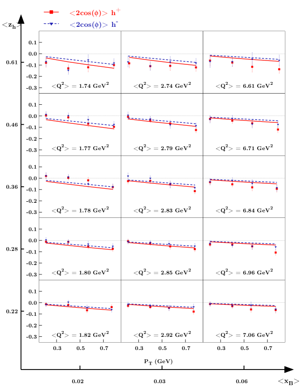
Figure 2: Best fit curves for $\langle\cos\phi\rangle\,$obtained by fitting COMPASS data on multiplicities, $\langle\cos\phi\rangle\,$and $\langle\cos 2\phi\rangle\,$. The Cahn effect in $\langle\cos 2\phi\rangle\,$has been set to zero.

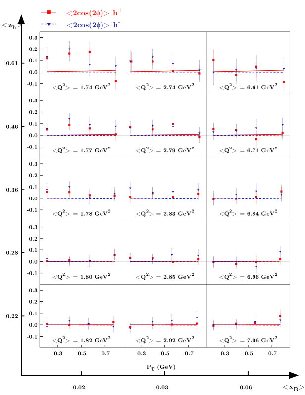
Figure 3: Best fit curves for $\langle\cos 2\phi\rangle\,$obtained by fitting COMPASS data on multiplicities, $\langle\cos\phi\rangle\,$and $\langle\cos 2\phi\rangle\,$. The Cahn effect in $\langle\cos 2\phi\rangle\,$has been set to zero.

In this paper we explore this configuration. We perform a global best fit which includes the multiplicities, the $\cos\phi$ asymmetry and the $\cos 2\phi$ asymmetry. Working up to order $1/Q$, these asymmetries read:

$$\begin{array}[]{l l}A^{\cos\phi}=\left.A^{\cos\phi}\right|_{\rm Cahn}+\left.A^{\cos\phi}\right|_{\rm BM}\\ \\ A^{\cos 2\phi}=\left.A^{\cos 2\phi}\right|_{\rm BM}\end{array}$$

As both COMPASS and HERMES data on $\langle\cos\phi\rangle$ and $\langle\cos 2\phi\rangle$ are restricted to a narrow $x$ range, they do not allow us to determine the precise $x$-dependence of the Boer–Mulders function. Thus we take $\Delta f_{q^{\uparrow}/p}$ to be simply proportional to $f_{q/p}$, by setting $\alpha_{q}=\beta_{q}=0$ in Eq. (18). For the Collins function, we distinguish a favored and a disfavored component, and we fix their parameters to the values obtained in a recent fit of the Collins asymmetries in SIDIS and $e^{+}e^{-}$ annihilation Anselmino:2013vqa :

$$N_{\rm fav}^{C}=0.49,\;\;\;N_{\rm disf}^{C}=-1.00,$$

$$\gamma=1.06,\;\;\;\delta=0.07,$$

$$M_{C}^{2}=1.50\;{\rm GeV}^{2}.$$ (46)

To parameterize the Boer–Mulders and Collins functions we need to input the unpolarized $f_{q/p}(x)$ and $D_{q/p}(z)$, see Eqs. (18) and (23). Consistently with our previous choice, Eqs. (15) and (16), we will use the collinear CTEQ6L distribution functions Pumplin:2002vw and DSS fragmentation functions  deFlorian:2007aj . As mentioned before, $\langle k_{\perp}^{2}\rangle=C$ and $\langle p_{\perp}^{2}\rangle=A+Bz_{h}^{2}$, with $A$, $B$ and $C$ free parameters to be determined by the fit.

It is known that the COMPASS multiplicities should be corrected by a large normalization factor: in fact, issues in that analysis were detected, which can affect the overall $x$, $y$, $z$ normalization of multiplicities up to 40%, as pointed out in Ref. Stolarski:2015 . Lacking for the moment the corrected data, in the present paper we apply the same multiplicative normalization factor as obtained in Anselmino:2013lza , $N_{y}=1.06-0.43\,y.$ This correction was found to improve considerably the fit of the COMPASS multiplicities.

The kinematical range explored by the two experiments is further restricted in order to make sure that our description, based on TMD factorization, can safely be applied. To avoid contaminations from exclusive hadronic production processes and large $z$ resummation effects Anderle:2012rq we select data with $z_{h}<0.65$ for COMPASS and with $z_{h}<0.69$ for HERMES. The lowest cut in $Q^{2}$ is chosen accordingly to the minimum $Q^{2}$ in the CTEQ6L analysis, $Q^{2}>1.69$ GeV², which amounts to excluding the lowest $x$ bins. Finally, we select $0.2<P_{T}<0.9\;{\rm GeV}$, following Ref. Anselmino:2013lza .

The results of the fit for the azimuthal moments are shown in Figs. 2 and 3, for the COMPASS data, and in Figs. 4 and 5, for the HERMES data. The description of the multiplicities is practically unchanged compared to Ref. Anselmino:2013lza , therefore we do not show the plots here. The values of $\chi^{2}$ and of the parameters are listed in Tables 1 and 2.

Table 1: Minimal $\chi^{2}$ and parameters, for a fit on COMPASS multiplicities, $\langle\cos\phi\rangle\,$and $\langle\cos 2\phi\rangle\,$in which the Cahn effect in $\langle\cos 2\phi\rangle\,$has been set to zero. Parameter errors correspond to a $2\sigma$ confidence level.

Cuts	$\chi^{2}$	Parameters
$z_{h}<0.65\,\,\,\,\,\,\,\,\,\,\,\,\,\,\,\,\,\,\,\,\,\,$	$\,(\chi^{2}_{pt})_{mult}\,=3.43$	$~{}~{}A=0.200\pm 0.002$	$~{}~{}M_{BM}^{2}=0.09\pm 0.45$
$Q^{2}>1.69\,\,\,\,\,\,\,\,\,\,\,\,\,\,\,\,\,\,\,\,\,\,$	$(\chi^{2}_{pt})_{cos(\phi)}=1.17$	$~{}~{}B=0.571\pm 0.018$	$~{}~{}N_{d}=-1.00\pm 1.95$
$0.2<P_{T}<0.9\,\,\,\,\,\,\,\,\,\,\,$	$(\chi^{2}_{pt})_{cos(2\phi)}=1.02$	$~{}~{}C=0.031\pm 0.006$	$~{}~{}N_{u}=-0.45\pm 0.26$

Table 2: Minimal $\chi^{2}$ and parameters, for a fit on HERMES multiplicities, $\langle\cos\phi\rangle\,$and $\langle\cos 2\phi\rangle\,$in which the Cahn effect in $\langle\cos 2\phi\rangle\,$has been set to zero. Parameter errors correspond to a $2\sigma$ confidence level.

Cuts	$\chi^{2}$	Parameters
$z_{h}<0.69\,\,\,\,\,\,\,\,\,\,\,\,\,\,\,\,\,\,\,\,\,\,$	$\,(\chi^{2}_{pt})_{mult}\,=1.70$	$A=0.126\pm 0.004$	$~{}~{}M_{BM}^{2}=0.10\pm 0.20$
$Q^{2}>1.69\,\,\,\,\,\,\,\,\,\,\,\,\,\,\,\,\,\,\,\,\,\,$	$(\chi^{2}_{pt})_{cos(\phi)}=2.39$	$B=0.506\pm 0.045$	$~{}~{}N_{d}=-1.00\pm 0.20$
$0.2<P_{T}<0.9\,\,\,\,\,\,\,\,\,\,\,$	$(\chi^{2}_{pt})_{cos(2\phi)}=2.13$	$C=0.037\pm 0.004$	$~{}~{}N_{u}=-0.49\pm 0.15$

The asymmetry data (especially $\langle\cos\phi\rangle\,$) drive the transverse momentum of quarks to a very small value, $\langle k_{\perp}^{2}\rangle\sim 0.03-0.04$ GeV², which means that the transverse momentum of the produced hadron is largely due to transverse motion effects in the fragmentation process. The difference between positive and negative hadrons is found to be small (or even negligible), and the agreement with the data on $\langle\cos\phi\rangle$ worsens as $z_{h}$ grows and $Q^{2}$ decreases.

One may wonder whether a more flexible model, including flavor dependent Gaussian widths, could modify our results. It would indeed be interesting to determine whether the available SIDIS data signal any flavor dependence in the unpolarized TMDs. This was already considered in the analysis of multidimensional multiplicities of Ref. Anselmino:2013lza , where it was noted that flavor dependence did not improve the description of the data significantly. Here we have performed several fits of the asymmetries allowing for flavor dependent parameters, but we have found that the overall picture does not improve. Furthermore including flavor dependence generates an over-parameterization, given the precision of present data, and consequently results in largely unconstrained fit solutions.

From Tables 1 and 2 one sees that the presence of the Boer–Mulders function is rather marginal: $\Delta f_{d^{\uparrow}/p}$ is very uncertain and compatible with zero, whereas $\Delta f_{u^{\uparrow}/p}$ is slightly more constrained, but very small.

The reason of this result is that our selection of multidimensional data on $\cos 2\phi$, which cuts out a large portion of data corresponding to small $Q^{2}$ values, turns out to be compatible with a zero asymmetry. Notice however that in the small $Q^{2}$ and large $z$ region the asymmetry is instead quite sizable. This can be seen also by considering the previous, one-dimensional data, where all variables but one are integrated over Kafer:2008ud ; Bressan:2009eu ; Giordano:2009hi . This means that the integrated asymmetries are mainly driven by small $Q^{2}$ and large $z$ events, which could be affected by relevant higher-twist contributions. The importance of the $\mathcal{O}(1/Q^{2})$ Cahn term, Eq. (29), was indeed pointed out in Ref. Barone:2009hw , but one should not forget that this term is only a part of the overall twist-four contribution, which is not explicitly known (at this order there are also target-mass effects, and the identification of $x_{B}$ and $z_{h}$ with the light-cone ratios $x$ and $z$ is no more valid).

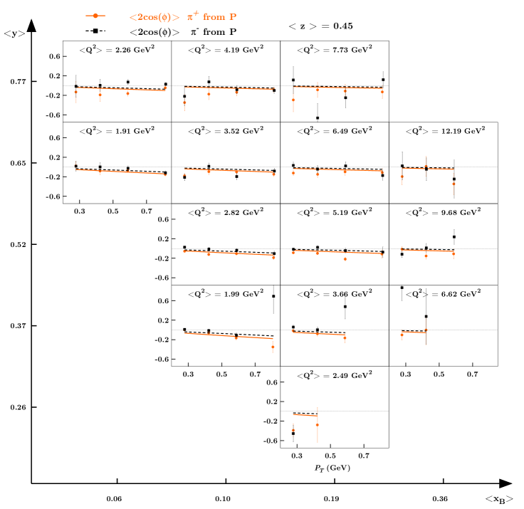
Figure 4: Best fit curves for $\langle\cos\phi\rangle\,$obtained by fitting HERMES data on multiplicities, $\langle\cos\phi\rangle\,$and $\langle\cos 2\phi\rangle\,$. The Cahn effect in $\langle\cos 2\phi\rangle\,$has been set to zero. Here we show only one bin in $z$, as an example, with $\langle z\rangle=0.45$

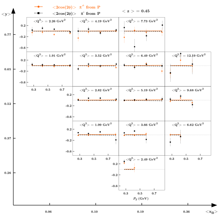
Figure 5: Best fit curves for $\langle\cos 2\phi\rangle\,$obtained by fitting HERMES data on multiplicities, $\langle\cos\phi\rangle\,$and $\langle\cos 2\phi\rangle\,$. The Cahn effect in $\langle\cos 2\phi\rangle\,$has been set to zero. Here we show only one bin in $z$, as an example, with $\langle z\rangle=0.45$

By inspecting the recent release of azimuthal asymmetries by HERMES Airapetian:2012yg and COMPASS Adolph:2014pwc , the difference between the sizes of the negative and positive hadron production asymmetries is evident in the one-dimensional data (see Figs. $14$–$16$ of Ref. Airapetian:2012yg and in Figs. $14$, $15$ of Ref. Adolph:2014pwc ); moreover, in this case both $A^{\cos\phi}$ and $A^{\cos 2\phi}$ are consistently different from zero. However, these same features are not readily visible in the multidimensional data sets.

At this stage we would like to understand whether we can assign a physical meaning to the extracted parameters. As a matter of fact, the values of the average momentum $\langle k_{\perp}^{2}\rangle$ extracted from our fit is quite different (one order of magnitude smaller) from that previously extracted in several different fits Anselmino:2005nn ; Signori:2013mda ; Anselmino:2013lza . This small value is mainly driven by the $\langle\cos\phi\rangle\,$asymmetry, which is entirely twist-three. It is clear that one should make sure to evaluate this asymmetry correctly in order to interpret the extracted parameter as the average momentum $\langle k_{\perp}^{2}\rangle$.

The Cahn and Boer–Mulders terms in $\langle\cos\phi\rangle$ can, in fact, be supplemented by other dynamical $1/Q$ contributions Bacchetta:2006tn . Taking quark-gluon correlations into account Eq. (9) acquires, for instance, an additional term containing a new distribution function, $\widetilde{f}_{q}$, and becomes

$$\left.F_{UU}^{\cos\phi}\right|_{\rm Cahn}=-2\sum_{q}e_{q}^{2}x\int{\mathrm{d}}^{2}\mbox{\boldmath$k$}_{\perp}\,\frac{(\mbox{\boldmath$k$}_{\perp}\cdot\mbox{\boldmath$h$})}{Q}[f_{q}(x,k_{\perp})+\widetilde{f}_{q}(x,k_{\perp})]D_{q}(z,p_{\perp}).$$ (47)

Notice that this new term cannot be separated from the other. A similar correction, with another distribution function $\widetilde{h}_{q}$, applies to the Boer–Mulders component (10), and the fragmentation functions should also be modified for quark-gluon correlations.

Whereas it is generally believed that the “tilde” $\mathcal{O}(1/Q)$ contributions are negligible, it is possible that in the kinematical regions presently explored this might not be the case. Possible cancellations among these terms could affect the extraction of the intrinsic momenta parameters.

In order to estimate the impact of the dynamical higher-twist contributions to the Cahn effect, we can simply assume tilde functions to be proportional to the non-tilde ones. Given the restricted kinematical ranges of the data, this is not a very limiting assumption. Thus the presence of $\widetilde{f}_{q}$ is effectively simulated by an extra normalization constant $N_{\rm Cahn}$ in front of the $\langle\cos\phi\rangle\,$Cahn term, that is:

$$A^{\cos\phi}=N_{\rm Cahn}\left.A^{\cos\phi}\right|_{\rm Cahn}+\left.A^{\cos\phi}\right|_{\rm BM}\,.$$

Since $\langle\cos\phi\rangle\,$is dominant in our fit, one sees from Eq. (26) that the effect of $N_{\rm Cahn}$ is compensated by a readjustment of $\langle k_{\perp}^{2}\rangle$ (which determines not only the width of the Gaussian distributions, but also the size of the asymmetries). Therefore, identical fits are obtained by allowing $N_{\rm Cahn}$ to be smaller than unity, and proportionally increasing $\langle k_{\perp}^{2}\rangle$. For instance, setting $N_{\rm Cahn}=0.5$, that is assuming that dynamical twist–3 terms reduce by 50% the Cahn term, one gets $\langle k_{\perp}^{2}\rangle=0.06$ GeV² (twice the value obtained in our main fit). An even larger cancellation, that is a smaller $N_{\rm Cahn}\sim 0.1$ coefficient, would deliver a value of $\langle k_{\perp}^{2}\rangle$ similar to those extracted in previous analyses Anselmino:2005nn ; Schweitzer:2010tt ; Signori:2013mda .

We conclude that in the present kinematics the structure and the magnitude of the higher–twist terms, which are not fully under control, are crucial for determining $\langle k_{\perp}^{2}\rangle$.

IV Conclusions and perspectives

In the TMD framework, the $\langle\cos\phi\rangle\,$and $\langle\cos 2\phi\rangle\,$asymmetries are sensitive to the transverse momentum of quarks inside the target and in the fragmentation process. In the Gaussian model of quark distributions, the widths $\langle k_{\perp}^{2}\rangle$ and $\langle p_{\perp}^{2}\rangle$ also determine the size of the asymmetries. Adopting an $\mathcal{O}(1/Q)$ scheme, which attributes $\langle\cos\phi\rangle\,$both to Cahn and Boer–Mulders effects at order $1/Q$, and $\langle\cos 2\phi\rangle\,$to the Boer–Mulders effect at leading twist, and ignoring twist-3 dynamical contributions (arising from quark–gluon correlations), our analysis shows that the recent COMPASS and HERMES multidimensional data can be reproduced by a very small value of $\langle k_{\perp}^{2}\rangle$, namely 0.03-0.04 GeV². Within this picture, this means that most of the transverse momentum of the outgoing hadron is due to the fragmentation, which must be described by a function with a $z$-dependent width. This result, mainly driven by $\langle\cos\phi\rangle\,$, could be modified by the presence of further twist–3 terms, which might not be negligible due to the relevance of the small-$Q^{2}$ region in the present measurements.

A somehow disappointing output of our fits is the indeterminacy on the extraction of the Boer–Mulders function, which seems to play a minor role in the asymmetries. This is seen in particular from $\langle\cos 2\phi\rangle\,$, which is entirely determined by the Boer–Mulders contribution but appears to be, within large errors, compatible with zero.

On the other hand, the integrated $\langle\cos 2\phi\rangle\,$data Airapetian:2012yg show a non vanishing asymmetry, especially when plotted against $z$. The asymmetry is slightly negative for $\pi^{+}$ and positive for $\pi^{-}$, as expected from the Boer–Mulders effect Barone:2008tn . Also the integrated data on $\langle\cos\phi\rangle\,$show a different asymmetry for $\pi^{+}$ and $\pi^{-}$: this indicates a flavor dependence which can only be achieved with a non-zero Boer–Mulders effect since, within a flavor–independent Gaussian model with factorized $x$ and $k_{\perp}$ dependences, the Cahn effect is flavor blind and can only generate identical contributions for positively or negatively charged pions. However, the signs of the $u$ and $d$ Boer–Mulders functions required for a successful description of $\langle\cos 2\phi\rangle\,$appear to be incompatible with those required to generate the appropriate difference between $\pi^{+}$ and $\pi^{-}$ in the $\langle\cos\phi\rangle\,$azimuthal moment. As we mentioned, a more refined model with flavor dependent Gaussian widths is not helpful, given the precision of the current experimental data.

One should not forget about the existence of other higher-twist effects that could combine with the Boer–Mulders term and alter the simple picture considered here. In order to disentangle these contributions, it might be useful to integrate the asymmetry data on restricted kinematical ranges, so as to avoid the low-$Q^{2}$ region and meet the requirements of TMD factorization. Analyzing properly integrated data could help to clarify the origin of azimuthal asymmetries and possibly to get more information on the Boer–Mulders function. Work along these lines is in progress.

It would also be interesting to investigate how SIDIS azimuthal modulations can be affected by gluon radiations. Following Ref. Chay:1991nh one can actually compute the perturbative corrections originating from gluon radiation at order $\alpha_{s}$ for the numerator and denominator of the azimuthal asymmetries. Indeed, in the limit of small $q_{T}$ (where our analysis applies) they are affected by strong divergences, generated by soft and collinear gluon radiation. One might expect that these divergences cancel out in the ratio when building the azimuthal asymmetry, but this only happens when the divergences appearing in the numerator and in the denominator are of the same origin and have the same structure. In fact, in a more recent paper Berger:2007jw , it is explicitly shown that, for Drell-Yan scattering processes, the $\langle\cos 2\phi\rangle\,$azimuthal modulation of the cross section shares with the azimuthal independent (integrated) term the same $q_{T}$ logarithmic behaviour of the asymptotic cross section, proportional to $(Q^{2}/q_{T}^{2})\ln(Q^{2}/q_{T}^{2})$. In this case the same resummation techniques which are known to work for the integrated cross section (which appear at denominator) can be applied to the azimuthal modulation appearing at numerator. However, they point out that this does not happen for the $\langle\cos\phi\rangle\,$azimuthal modulation, which does not exhibit the usual diverging logarithmic term, but is simply proportional to $(Q^{2}/q_{T}^{2})$. In this case, the usual resummation scheme techniques cannot be applied and new strategies needs to be devised. To the best of our knowledge, this has not been explicitly studied for SIDIS processes, where applying usual resummation schemes and conventional matching recipes is much more problematic, even in the simplest case of integrated, unpolarized cross sections Boglione:2014oea .

References

(1)
H. Georgi and H. D. Politzer,
Phys. Rev. Lett. 40, 3 (1978).
(2)
A. Mendez,
Nucl. Phys. B145, 199 (1978).
(3)
R. N. Cahn,
Phys. Lett. B78, 269 (1978).
(4)
R. N. Cahn,
Phys. Rev. D40, 3107 (1989).
(5)
A. Konig and P. Kroll,
Z. Phys. C16, 89 (1982).
(6)
J.-g. Chay, S. D. Ellis, and W. J. Stirling,
Phys. Rev. D45, 46 (1992).
(7)
V. Barone, F. Bradamante, and A. Martin,
Prog.Part.Nucl.Phys. 65, 267 (2010), arXiv:1011.0909.
(8)
X.-d. Ji, J.-p. Ma, and F. Yuan,
Phys. Rev. D71, 034005 (2005), arXiv:hep-ph/0404183.
(9)
European Muon, J. J. Aubert et al.,
Phys. Lett. B130, 118 (1983).
(10)
European Muon, M. Arneodo et al.,
Z. Phys. C34, 277 (1987).
(11)
ZEUS, J. Breitweg et al.,
Phys. Lett. B481, 199 (2000), arXiv:hep-ex/0003017.
(12)
D. Boer and P. J. Mulders,
Phys. Rev. D57, 5780 (1998), arXiv:hep-ph/9711485.
(13)
COMPASS Collaboration, W. Kafer,
(2008), arXiv:0808.0114.
(14)
COMPASS Collaboration, A. Bressan,
(2009), arXiv:0907.5511.
(15)
HERMES Collaboration, F. Giordano and R. Lamb,
AIP Conf.Proc. 1149, 423 (2009), arXiv:0901.2438.
(16)
V. Barone, S. Melis, and A. Prokudin,
Phys.Rev. D81, 114026 (2010), arXiv:0912.5194.
(17)
V. Barone, A. Prokudin, and B.-Q. Ma,
Phys.Rev. D78, 045022 (2008), arXiv:0804.3024.
(18)
HERMES Collaboration, A. Airapetian et al.,
Phys.Rev. D87, 074029 (2013), arXiv:1212.5407.
(19)
COMPASS, C. Adolph et al.,
Eur.Phys.J. C73, 2531 (2013), arXiv:1305.7317.
(20)
HERMES Collaboration, A. Airapetian et al.,
Phys.Rev. D87, 012010 (2013), arXiv:1204.4161.
(21)
COMPASS Collaboration, C. Adolph et al.,
Nucl.Phys. B886, 1046 (2014), arXiv:1401.6284.
(22)
P. Schweitzer, T. Teckentrup, and A. Metz,
Phys.Rev. D81, 094019 (2010), arXiv:1003.2190.
(23)
LHPC Collaboration, B. U. Musch et al.,
PoS LAT2007, 155 (2007), arXiv:0710.4423.
(24)
J. Pumplin et al.,
JHEP 0207, 012 (2002), arXiv:hep-ph/0201195.
(25)
D. de Florian, R. Sassot, and M. Stratmann,
Phys.Rev. D75, 114010 (2007), arXiv:hep-ph/0703242.
(26)
M. Anselmino, M. Boglione, J. Gonzalez H., S. Melis, and A. Prokudin,
JHEP 1404, 005 (2014), arXiv:1312.6261.
(27)
M. Anselmino et al.,
Phys.Rev. D87, 094019 (2013), arXiv:1303.3822.
(28)
COMPASS Collaboration, M. Stolarski,
Contribution to the 21st International Symposium on Spin Physics
(SPIN 2014), October 20-24, 2014, Beijing, China (2015).
(29)
D. P. Anderle, F. Ringer, and W. Vogelsang,
Phys.Rev. D87, 034014 (2013), arXiv:1212.2099.
(30)
M. Anselmino et al.,
Phys.Rev. D71, 074006 (2005), arXiv:hep-ph/0501196.
(31)
A. Signori, A. Bacchetta, M. Radici, and G. Schnell,
JHEP 1311, 194 (2013), arXiv:1309.3507.
(32)
A. Bacchetta et al.,
JHEP 0702, 093 (2007), arXiv:hep-ph/0611265.
(33)
E. L. Berger, J.-W. Qiu, and R. A. Rodriguez-Pedraza,
Phys.Rev. D76, 074006 (2007), arXiv:0708.0578.
(34)
M. Boglione, J. O. G. Hernandez, S. Melis, and A. Prokudin,
JHEP 1502, 095 (2015), arXiv:1412.1383.