Wavelet-based cross-correlation analysis of structure scaling in turbulent clouds

Abstract

Aims. We propose a statistical tool to compare the scaling behaviour of turbulence in pairs of molecular cloud maps. Using artificial maps with well defined spatial properties, we calibrate the method and test its limitations to ultimately apply it to a set of observed maps.

Methods. We develop the wavelet-based weighted cross-correlation (WWCC) method to study the relative contribution of structures of different sizes and their degree of correlation in two maps as a function of spatial scale, and the mutual displacement of structures in the molecular cloud maps.

Results. We test the WWCC for circular structures having a single prominent scale and fractal structures showing a self-similar behavior without prominent scales. Observational noise and a finite map size limit the scales where the cross-correlation coefficients and displacement vectors can be reliably measured. For fractal maps containing many structures on all scales, the limitation from the observational noise is negligible for signal-to-noise ratios $\ga 5$. We propose an approach for identification of correlated structures in the maps which allows us to localize individual correlated structures and recognize their shapes and suggest a recipe for the recovering of enhanced scales in self-similar structures. Application of the WWCC to the observed line maps of the giant molecular cloud G 333 allows to add specific scale information to the results obtained earlier using the principle component analysis (PCA). It confirms the chemical and excitation similarity of ¹³CO and C¹⁸O on all scales, but shows a deviation of HCN at scales of up to 7 pc. This can be interpreted as a chemical transition scale. The largest structures also show a systematic offset along the filament, probably due to a large-scale density gradient.

Conclusions. The WWCC can compare correlated structures in different maps of molecular clouds identifying scales that represent structural changes such as chemical and phase transitions and prominent or enhanced dimensions.

1 Introduction

The interstellar medium has a complex dynamic structure on all scales (from sub-parsecs to at least tens of parsecs) as a result of various physical processes occurring in the multi-scale turbulent cascade of molecular and atomic gas. High-resolution and high dynamic range of observations of emission line transitions and continuum emission of interstellar clouds provide evidence for clumpy structures on all scales (see e.g. Stutzki & Guesten 1990; Roman-Duval et al. 2011) and anisotropic clouds such as shells and filaments (e.g. Men’shchikov et al. 2010; Deharveng et al. 2010). Observations of line transitions, total and polarized continuum emission provide valuable information about physical conditions (density, temperature, magnetic field) and kinematics of a multi-phase gas distributed on different scales.

The correlation between different structures measured in interstellar clouds, e.g. contours of different chemical tracers or the density, temperature and velocity peaks, as a function of their size can be used to quantify commonalities and differences in the formation of these structures. Understanding the commonalities and differences seen in different tracers, different velocity components or different excitation conditions as a function of scale length, will help to infer the underlying physical processes in the turbulent cascade in interstellar clouds. As many processes have characteristic scales, but show their signatures only in particular tracers, it is essential to compare the scaling behaviour of various tracers in a same region to identify those scales. The characteristic scales could be, e.g., chemical transition scales (see, e.g., Glover et al. 2010), when comparing molecular line maps of different species, dynamical scales for the formation of coherent structures (Goodman et al. 1998), IR penetration scales showing up in dust continuum maps at different wavelengths (e.g. Abergel et al. 1996), ambipolar diffusion scales for the dynamical coupling between ionized and neutral particles, seen when comparing maps of ionized and neutral species (McKee et al. 2010; Li et al. 2012), and dissipation scales when comparing channel maps of individual atomic or molecular lines (Falgarone et al. 1998).

To address these issues, we use two different starting points. The wavelet analysis has been proven to be a powerful tool for detecting structures on different spatial scales in time-series and in 2-dimensional maps. It was used e.g. in the $\Delta$-variance analysis measuring the amount of structure in a molecular cloud map as a function of scale and to determine the slope of the power spectrum of the cloud scaling (Stutzki et al. 1998). A combination of a wavelet filtering with the cross-correlation function was first proposed by Nesme-Ribes et al. (1995) to study the solar activity. Frick et al. (2001) improved the method introducing the wavelet cross-correlation function to study the correlation between galactic images as a function of scale. This method and its modifications were successfully applied to study solar physics, ionosphere fluctuations, images of astronomical objects and all-sky surveys (e.g., Vielva et al. 2006; Liu & Zhang 2006; Tabatabaei & Berkhuijsen 2010; Roux et al. 2012; Tabatabaei et al. 2013).

These approaches, however, are not designed for recovering the displacement of structures in the data sets on scale-by-scale basis and accounting for a variable noise distribution across the maps and irregular boundaries. Patrikeev et al. (2006) used an anisotropic wavelet transform to isolate spiral features in images of M 51 for different tracers and analysed their location and pitch angle as a function of radius and azimuth but they did not cross-correlate the features seen in different tracers. The wavelet-based cross-correlation method can be improved by inheriting the corresponding formalism from the wavelet-based $\Delta$-variance analysis and combining it with the cross-correlation analysis. To account for an uneven distribution of noise in the maps, Ossenkopf et al. (2008a) (hereafter O08) implemented a weighting function in the improved $\Delta$-variance method to analyse arbitrary data sets of molecular clouds. The weighting function corrects for the contribution of data points with a varying signal-to-noise ratio as well as allows to perform a proper treatment of map edges, independent of their shape, and calculations in Fourier space and, hence, speeds up the computation by making use of the fast Fourier transform. Moreover, O08 suggested an optimal shape of the wavelet filter for analysing the turbulent structures.

In this paper, we make use of the advantages of weighting functions and develop a weighted wavelet cross-correlation (WWCC) method to recover the correlation and displacement between structures of molecular clouds as a function of scale, in which no assumption about the noise or boundaries are made.

The paper is organised as follows. Section 2 introduces the $\Delta$-variance and cross-correlation methods. The WWCC method is presented in Sect. 3. Application of the WWCC to simulated circular structures and fractal structures is described in Sect. 4. Application of the WWCC to observed emission line maps of the giant molecular cloud G 333 is presented in Sect. 5. Discussion and conclusions are presented in Sect. 6.

2 Basic theory

We consider two maps, $f(\@vec{x})$ and $g(\@vec{x})$, $(\@vec{x}=(x,y))$, weighted at each pixel by a significance function $w_{f}(\@vec{x})$ and $w_{g}$($\@vec{x}$). The significance functions $w_{f}(\@vec{x})$ and $w_{g}(\@vec{x})$ characterize e.g. a variable signal-to-noise ratio across the maps or can be used to treat irregular map boundaries.

2.1 Wavelet analysis to measure the scaling in turbulent structures

The $\Delta$-variance measures the amount of structure in an individual map as a function of scale, thereby identifying dominant structure sizes. In this context “structure” describes the spatial variation of measured properties, i.e. a deviation from a flat or zero measurement. The amount of structures quantifies the total variation in a given map as characterized by the variance. With the $\Delta$-variance, this is evaluated as a function of the size of the structures equivalent to the power spectrum (Stutzki et al. 1998). This method represents a 2-dimensional generalisation of the Allan-variance method (Allan 1996). The $\Delta$-variance is evaluated from the map $f$ convolved with the wavelet $\psi$

$$F(\@vec{x},l)=f(\@vec{x})\ast\psi({\@vec{x}},l)=\mathop{\int\!\!\!\int}_{x,y}f({\@vec{x}^{\prime}})\psi({\@vec{x}^{\prime}}-{\@vec{x}},l)d{\@vec{x}^{\prime}},$$ (1)

by computing its variance

$$\sigma^{2}_{\Delta}(l)=\mathop{\int\!\!\!\int}_{x,y}[F(\@vec{x},l)-\overline{F}(l)]^{2}d\@vec{x},$$ (2)

where the $\ast$ symbol represents the convolution and $\overline{F}(l)$ is the average intensity of the map. For uniform, zero average data without boundaries, this is equivalent to the wavelet power spectrum.

The wavelet is composed of a positive core, $\psi_{\rm c}$, and a negative annulus, $\psi_{\rm a}:$

$$\psi({\@vec{x}},l)=\psi_{c}({\@vec{x}},l)+\psi_{a}({\@vec{x}},l).$$ (3)

Core and annulus are normalized to an integrated weight of unity, so that the integral over the whole wavelet cancels to zero.

For a fast computation of the convolution in Eq. (1) Stutzki et al. (1998) used the multiplication in Fourier space, but Bensch et al. (2001) showed that this can lead to considerable errors from edge effects due to the incompatibility of the implicit assumption of periodic maps in the Fourier transform and the boundaries of real observed maps. They suggested a filter that changes its shape closer to the map boundaries by truncating it beyond the map edges and changing the amplitude of core and annulus to retain the wavelet normalization condition. While this improves the edge treatment its weakness is that the convolution of the map cannot be performed in Fourier space any more.

Ossenkopf et al. (2008a) suggested a modification that overcomes the edge treatment problems, simultaneously deals with the effect of observational uncertainties and irregular map boundaries, and allows for a computation in the Fourier domain. To fix the filter function they increase the map size when the filter extends beyond the map edges and apply a zero-padding to the extended map area. The re-normalization of the filter is accomplished by introducing the complementary weighting function $w(\@vec{x})>0$ inside the valid map and $w(\@vec{x})=0$ in the zero-padded region. When using a generalized weighting function $0\leq w(\@vec{x})\leq 1$ this can characterize the significance of every individual data point, including the effects of noise and observational uncertainties. Then the map $f_{\rm p}$ and the weights $w(\@vec{x})$ have to be convolved separately with the positive and negative filter parts $f_{\rm c}(\@vec{x},l)=f_{\rm p}\ast\psi_{c}({\@vec{x}},l)$, $f_{\rm a}(\@vec{x},l)=f_{\rm p}\ast\psi_{a}({\@vec{x}},l)$, $w_{\rm c}(\@vec{x},l)=w(\@vec{x})\ast\psi_{c}({\@vec{x}},l)$, and $w_{\rm a}(\@vec{x},l)=w(\@vec{x})\ast\psi_{a}({\@vec{x}},l)$ and the re-normalization is performed when computing the map filtered on scale $l$

$$F(\@vec{x},l)=\frac{f_{\rm c}(\@vec{x},l)}{w_{\rm c}(\@vec{x},l)}-\frac{f_{\rm a}(\@vec{x},l)}{w_{\rm a}(\@vec{x},l)}.$$ (4)

When finally computing the $\Delta$-variance from the convolved map, the weights are taken into account in the sum of the variations (O08):

$$\sigma^{2}_{\Delta}(l)=\frac{\mathop{\int\!\!\!\int}_{x,y}[F(\@vec{x},l)-\overline{F}_{w}(l)]^{2}w_{F}(\@vec{x},l)d\@vec{x}}{\mathop{\int\!\!\!\int}_{x,y}w_{F}(\@vec{x},l)\,d\@vec{x}},$$ (5)

with

$$w_{F}=w_{c}(\@vec{x},l)\,w_{a}(\@vec{x},l),$$ (6)

and $\overline{F}_{w}(l)$ as the weighted average of the map

$$\overline{F}_{w}(l)=\frac{\mathop{\int\!\!\!\int}w_{F}(\@vec{x},l)F(\@vec{x},l)\,d\@vec{x}}{\mathop{\int\!\!\!\int}w_{F}(\@vec{x},l)\,d\@vec{x}}.$$ (7)

The choice of the wavelet filter and its optimisation is of great importance for the scaling analysis. For isotropic wavelets, the ratio of the core diameter to annulus diameter is the critical parameter. O08 found that both, French-hat and Mexican-hat filters with a high ratio between the diameter of the annulus and the core of the filter, are preferred for measurements of the general power spectral slope, while the Mexican-hat filter with low diameter ratios is more suited to sensitively detect individual prominent scales. The Mexican-hat filter with an annulus/core diameter ratio of $v=1.5$ was found to provide the best compromise, revealing the correct power spectrum slope and all spectral features. Therefore, we will use this optimal wavelet filter (Eq. (11) in O08) throughout the rest of the paper:

$$\psi_{c}({\@vec{x}}) = \frac{4}{\pi l^{2}}\exp\left(\frac{-{\@vec{x}}^{2}}{(l/2)^{2}}\right)$$

$$\psi_{a}({\@vec{x}}) = -\frac{4}{\pi l^{2}(v^{2}-1)}\left[\exp\left(\frac{-{\@vec{x}}^{2}}{(vl/2)^{2}}\right)-\exp\left(\frac{-{\@vec{x}}^{2}}{(l/2)^{2}}\right)\right],$$ (8)

where $l$ is the scale of interest. The choice of the Gaussian smoothed filter is justified by the simultaneous confinement of the filter in ordinary and Fourier space. The usable range of scales $l$ falls between 2 pixels, needed to guarantee a reasonably isotropic filter shape on a rectangular pixel grid, and about half the map size as discussed in Sect. 4.1.2. The method was proven to be a powerful tool to characterise the power spectrum of interstellar clouds (Stutzki et al. 1998; Ossenkopf et al. 2008b).

2.2 Cross-correlation

We can compute the cross-correlation coefficient between two images or maps $f(\@vec{x})$ and $g(\@vec{x})$ as

$$r=\mathop{\int\!\!\!\int}_{x,y}f(\@vec{x})g(\@vec{x})\,d\@vec{x}.$$ (9)

describing the degree of concordance between the maps. If all structures are shifted between the two maps, the cross-correlation coefficient drops, but the characterization of the similarity of the two maps can be recovered when introducing a reverse offset vector $t$ while computing the cross-correlation. This leads to the definition of the two-dimensional cross-correlation function as a function of the offset vector, $\@vec{t}$, as

$$C(\@vec{t})=\mathop{\int\!\!\!\int}_{x,y}f(\@vec{x})g(\@vec{x}+\@vec{t})\,d\@vec{x}.$$ (10)

To account for different absolute scales in the maps one normalizes the cross-correlation function

$$C(\@vec{t})=\frac{\mathop{\int\!\!\!\int}_{x,y}(f(\@vec{x})-\overline{f})(g(\@vec{x}+\@vec{t})-\overline{g})\,d\@vec{x},}{\sigma_{f}\,\sigma_{g}},$$ (11)

where $\overline{f}$ and $\overline{g}$ are the means of signals in two maps, respectively, $\sigma_{f}$ and $\sigma_{g}$ are the standard deviations computed as,

$$\sigma_{f}=\left(\mathop{\int\!\!\!\int}_{x,y}(f(\@vec{x})-\overline{f})^{2}\,d\@vec{x}\right)^{1/2},$$ (12)

for $\sigma_{f}$ and equivalently for $\sigma_{g}$. The normalized cross correlation function has values between $-1$ and $+1$.

For every given offset vector $\@vec{t}$, the cross-correlation function measures the similarity (or correlation) between structures in the two maps, when the second map is shifted by $\@vec{t}$. The correlation function for a zero shift, $\@vec{t}=0$, recoveres the cross-correlation coefficient,

$$r=C(\@vec{t}=0)$$ (13)

as the center of the cross-correlation plane.

The position of the maximum of the cross-correlation function in the $\@vec{t}$ plane indicates the recovered displacement vector between the two maps, i.e. the applied offset for which the two structures match best. We compute the displacement vector as

$$\@vec{\tau}=\operatorname{arg}\,{\underset{x,y}{\operatorname{max}}\;}{C(\@vec{t})}.$$ (14)

The cross-correlation function between two images always integrates over all scales involved in the map, not distinguishing the correlation or mutual displacement of structures at particular scales. This is addressed by the wavelet cross-correlation.

3 Weighted wavelet cross-correlation

3.1 Theory

To study the dependence of the correlation coefficient on the spatial scale, the two data sets are filtered on scale-by-scale basis by means of wavelets and then cross correlated at each scale (see e.g., Frick et al. 2001).

Here, we introduce the weighted wavelet cross-correlation method to analyse the correlation between maps, $f$ and $g$, weighted at each pixel by $w_{f}$ and $w_{g}$, as a function of scale. For the filtering, the same formalism is exploited as for the $\Delta$-variance, i.e. Eq. (8) gives the wavelet to filter the maps on scale $l$ through Eq. (4) to obtain the filtered maps $F(\@vec{x},l)$ and $G(\@vec{x},l)$, and the convolved total weights at each pixel, $w_{F}(\@vec{x},l)$ and $w_{G}(\@vec{x},l)$, are computed through Eq. (6).

To study the cross correlation of the structure in two maps, $f$ and $g$, as a function of scale, we introduce the weighted wavelet cross-correlation function,

$$C_{w}(\@vec{t},l)=\frac{C_{F-G}(\@vec{t},l)}{\sigma_{w,F}(l)\,\sigma_{w,G}(l)},$$ (15)

where $C_{F-G}$ is the weighted covariance

$$C_{F-G}(\@vec{t},l) = \mathop{\int\!\!\!\int}_{x,y}\left(w_{F}(\@vec{x},l)\,F_{w}(\@vec{x},l)\right)\times$$ (16)

$$w_{G}(\@vec{x}+\@vec{t},l)\,G_{w}(\@vec{x}+\@vec{t},l)\,d\@vec{x},$$

with

$$F_{w}(\@vec{x},l)=F(\@vec{x},l)-\overline{F}_{w}(l),$$ (17)

and equivalently for $G_{w}(\@vec{x},l)$ where $\overline{F}_{w}(l)$ and $\overline{G}_{w}(l)$ are computed from Eq. (7). The normalization is given by the standard deviation

$$\sigma_{w,F}(l)=\left(\mathop{\int\!\!\!\int}_{x,y}w_{F}^{2}(\@vec{x},l)\,F_{w}^{2}(\@vec{x},l)\,d\@vec{x}\right)^{1/2},$$ (18)

of the $F_{w}$ map. $\sigma_{w,G}(l)$ is equivalently computed for $G_{w}$. The normalization WWCC function $C_{w}(\@vec{t},l)$ provides values between $-1$ and $+1$.

The WWCC is therefore a three-dimensional function depending on the offset vector $\@vec{t}$ and the filter size $l$. In the center of the offset plane, $\@vec{t}=0$, the WWCC function provides the wavelet cross-correlation coefficient $r(l)$, i.e. the degree of correlation of the two data sets on scale $l$,

$$r(l)=C_{w}(\@vec{t}=0,l).$$ (19)

The position of the maximum of the WWCC in the offset plane gives the optimum offset vector (for scale $l$) at which the maps are best aligned. We introduce the wavelet displacement vector,

$$\@vec{\tau}(l)=\operatorname{arg}\,{\underset{x,y}{\operatorname{max}}\;}{C_{w}(\@vec{t},l)},$$ (20)

which defines the amplitude and direction of displacement between two maps on scale $l$. These can be split into the spatial displacement function,

$$\tau(l)=(\tau_{x}^{2}+\tau_{y}^{2})^{1/2},$$ (21)

where $\tau_{x}$ and $\tau_{y}$ are offsets along $x$-axis and $y$-axis, and the angular displacement function,

$$\varphi(l)=\arctan\left(\frac{\tau_{y}}{\tau_{x}}\right).$$ (22)

For an efficient computation of the WWCC, the convolution in Eq. (16) can be obtained through a multiplication in Fourier space when transforming the weighted functions

$$\hat{F}_{w}(\@vec{k},l)=\mathop{\int\int}w_{F}(\@vec{x},l)\,F_{w}(\@vec{x},l)\,e^{-i\@vec{k}\@vec{x}}d\@vec{x},$$ (23)

$$\hat{G}_{w}(\@vec{k},l)=\mathop{\int\int}w_{G}(\@vec{x},l)\,G_{w}(\@vec{x},l)\,e^{-i\@vec{k}\@vec{x}}d\@vec{x},$$ (24)

where $\@vec{k}=(k_{x},k_{y})$ is the wavevector. Using the translational properties of the Fourier transform $\mathcal{F}$

$$\mathcal{F}\{w_{G}(\@vec{x}+\@vec{t},l)\,G_{w}(\@vec{x}+\@vec{t},l)\}=\hat{G}_{w}(\@vec{k},l)\times e^{i\@vec{k}\@vec{t}}$$ (25)

we can compute the integral for the WWCC function in Eq. (15) through the inverse Fourier transform $\mathcal{F}^{-1}\{\}$

$$C_{w}(\@vec{t},l)=\frac{\mathcal{F}^{-1}\{\hat{F}_{w}(\@vec{k},l)\hat{G}_{w}(\@vec{k},l)\times\exp{i\@vec{k}\@vec{t}}\}}{\sigma_{w,F}(l)\,\sigma_{w,G}(l)}.$$ (26)

3.2 Algorithm to compute the WWCC

The WWCC is computed for two images $f$ and $g$ and their weighting functions, $w_{f}$ and $w_{g}$, through the following steps:

1. Generate the weighted filtered maps for a given scale $l$, $F(\@vec{x},l)$ and $G(\@vec{x},l)$, using the convolution of $f$ and $g$ maps with the filter (Eqs. (4), (3) and (8)).

2. Compute the combined wavelet-filtered weights, $w_{F}$ and $w_{G}$ (Eq. (6)).

3. Calculate the $\Delta$-variance (Eq. (5)).

4. Compute the WWCC function (the degree of correlations for all possible displacements) on a given scale in Fourier domain (Eqs. (26,23,24)).

5. Determine the wavelet cross-correlation coefficient and wavelet displacement vector (Eqs. (19) and (20–22), respectively).

6. Repeat the steps 1–5 for every scale, $l$.

4 Testing the analytic power and limitations of the weighted wavelet cross-correlation

In this section we test the WWCC method by applying it to various sets of well-defined artificial maps to answer three questions:

• Can we determine individual characteristic scales in the two maps?

• Can we reproduce a given displacement of structures at particular scales?

• Can we trace a systematic change of the scale sizes between the two maps?

To address these questions, we use two different basic sets of simulated noisy maps. In one case, we assume Gaussian intensity profiles of a given size, representing individual smooth clumps. Then we have only one well-known prominent scale in the two maps to be compared and we can test the detection of a possible scale difference and a displacement of the structures. The other set of data is given by self-similar fractional Brownian motion structures (fBm, Peitgen & Saupe 1988). They do not have any dominant scale, but are characterized by a power-law distribution of scales. They can be described by a power law power spectrum of fractal structures and random phases in Fourier space. Here, we can test whether any scale dependent modifications (smoothing, displacement, …) are recovered by the WWCC. The two test cases (circular and fBm structures) should eventually represent limiting cases for the actual observations of molecular clouds. In one extreme view, maps are described as a collection of “spherical blobs”, in the other extreme they are described as scale-free, fully self-similar fractals. In practice, they typically contain both aspects, i.e. we find both self-similar structures and individual characteristic resolved structures.

For these test cases, we investigate the CC coefficient and displacement vector when changing the properties of the artificial clouds, such as the size of the individual structures, the spectral index of the self-similar scaling law, and the assumed noise level of the observations to test their sensitivity to those properties. The map size of all test data sets is $128\times 128$ pixels (abbreviated as pix throughout the rest of the paper).

4.1 Structures having Gaussian intensity profiles

We test the WWCC method for circular structures having Gaussian intensity profiles and some spatial displacement to study the effect of the size of circular structures and the noise level on the correlation coefficient and the measured displacement vector as a function of scale.

The Gaussian intensity profile is generated with an amplitude equal to unity and width given by standard deviation $\sigma$. A weight (significance value) of unity is assigned to each data point (pixel) in the map.

(a)
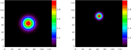
(b)

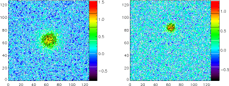
Figure 1: (a) Maps of two circular Gaussian structures ($\sigma_{1}=10$ pix and $\sigma_{2}=5$ pix) shifted by 20 pix along $y$-axis. (b) Observed with a simulated $\mathrm{S/N}=5$.

In Fig. 1 we show two pairs of test maps given by circular Gaussian structures (with $\sigma_{1}=10$ pix and $\sigma_{2}=5$ pix and a displacement of the peak by $\@vec{\tau}_{i}=20$ pix along $y$-axis in the second map). As the cross-correlation (Eqs. (10) and (15)) only considers the relative offset of structures between two maps, $\@vec{t}$, the result is invariant with respect to an exchange of negative offsets in map 1 by positive offsets in map 2. The WWCC always characterizes the mutual displacement of structures within the two considered data sets. Here, we always displace the structure in the second map relative to the first one. The upper panels show the original structure representing a $\mathrm{S/N}=\infty$, the lower panels are superimposed by white noise simulating typical observations with $\mathrm{S/N}=5$, i.e. $\sigma_{\rm noise}=0.2$.

(a) (b)

Figure 2: Maps of the two Gaussians with $\mathrm{S/N}=5$ from Fig. 1b filtered on scale of 5 pix (a) and of 45 pix (b). To allow for a filtering in Fourier space, the maps are extended beyond the original boundaries before filtering. The extension is treated with $w_{F}=0$ in the computation.

4.1.1 Map filtering

The first step in the analysis is the wavelet convolution (Eq. (1)) filtering the maps on a given scale. The usable range of the filter sizes is inherited from the $\Delta$-variance analysis discussed in Sect. 2.1. It starts at a resolution of two pixels. Fig. 2 shows the result, $F(\@vec{x},l)$ and $G(\@vec{x},l)$ for the $\mathrm{S/N}=5$ case for two selected wavelet filter sizes $l=5$ pix and $l=45$ pix. The filtered maps are larger than the original ones to allow for a convolution with non-truncated wavelets (see O08). The extension is treated with zero weighting in the further computation. We see that the maps filtered on small scales (5 pix) are dominated by noise, while the structures filtered on large scales (45 pix) are basically free of noise. Statistically, the noise will dominate the cross correlation for all scales $l$ below a critical size. This size depends on signal to noise level and will be discussed later in this section.

Figure 3: $\Delta$-variance spectra of the two Gaussians with $\mathrm{S/N}=\infty$ from Fig. 1 (a). The $\Delta$-variance spectra of the large (left) and small (right) circular structures (Fig. 1 (a)) are denoted by full and dotted lines respectively. Vertical thick lines are used to denote the measured prominent scales of the large and small circular structures, respectively.

4.1.2 The $\Delta$-variance spectrum

Computing the variance of the wavelet-filtered maps for all filter sizes leads to the $\Delta$-variance spectra ($\sigma^{2}_{\Delta}(l)$; Eq. (5)). Fig. 3 shows the resulting spectra for the original maps without noise and Fig. 4 the spectra for the case with $\mathrm{S/N}=5$. The $\Delta$-variance characterises the amount of structure distributed on different spatial scales. The peaks of $\Delta$-variance spectra indicate the dominant structure size. For structures without additional small scale contributions, the $\Delta$-variance falls off like $l^{4}$ below the dominant size. This is well seen in Fig. 3 for scales below about 8 pix. The increasing statistical uncertainty of the $\Delta$-variance for larger scales due to the lower number of statistically independent entities of large scales in the maps practically limits the use of the $\Delta$-variance analysis to prominent sizes of less than half of the map size (O08). The huge formal error bars in Fig. 3 following O08 are irrelevant here, as they characterize the counting statistics of individual structures, being very bad for a single structure in an otherwise empty map, while every observed map typically contains much more structure.

The $\Delta$-variance detects the prominent scales of the circular structures at $l_{\rm p1}=41$ pix and $l_{\rm p2}=18$ pix (vertical lines in Fig. 3). This corresponds approximately to the diameter of the circles visible in colors in Fig. 1 (a), i.e. at a level above 10 % of the peak intensity. For isotropic structures, the prominent scale approximately identifies the visible size of the structure (Mac Low & Ossenkopf 2000). We find a fixed relation between the prominent scale and the standard deviation of a circular structure $l_{\rm p}\approx 4\sigma$.

Figure 4: $\Delta$-variance spectra of the two Gaussians with $\mathrm{S/N}=5$ from Fig. 1 (b). The $\Delta$-variance spectra of the large (left) and small (right) circular structures (Fig. 1 (b)) are denoted by full and dotted lines respectively. Vertical thick lines denote the measured prominent scales of the large and small circular structures, respectively.

When we compute the $\Delta$-variance spectra of the same structures simulated with $\mathrm{S/N}=5$ (Fig. 4) we find a superimposed structure on scales less than 8 pix which is due completely to noise. The noise contribution decreases with $\sigma^{2}_{\Delta}(l)\propto l^{-2}$ (see Bensch et al. 2001) up to $\approx 8$ pix and becomes negligible towards larger scales as discussed for the map filtering above, leading to a $\Delta$-variance minimum at a scale of about 8 pix here. At scales above the minimum the spectra behave identical to Fig. 3 and reach the maxima at scales of 41 pix and 18 pix.

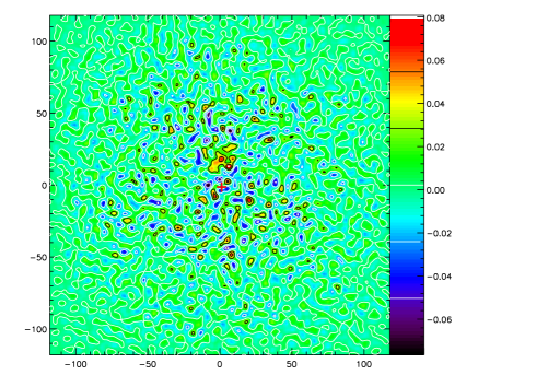
(a) (b)

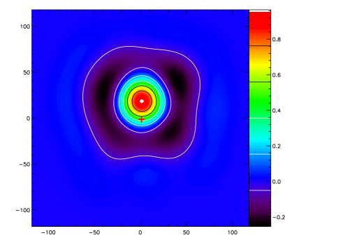
Figure 5: Cross-correlation functions for the pairs of wavelet-filtered maps from Fig. 2. The top panel (a) shows $C_{w}({\@vec{t}},5$pix), the bottom panel (b) $C_{w}({\@vec{t}},45$pix). The red crosses denote the center of the offset plane $\@vec{t}=0$, where one can read the wavelet cross-correlation coefficient $r(l)=C_{w}(\@vec{t}=0,l)$. The peak of the cross-correlation functions is displaced from the center by $\tau(l)=\tau_{i}$ as the WWCC recovers the input displacement of the structure in the second map.

4.1.3 The WWCC function

The WWCC map is finally computed through Eq. (26) providing the correlation for all possible displacements on a given scale. It is then used to compute the CC coefficient and displacement vector as a function of scale. The center of the WWCC map represents the correlation of the two structures not correcting for any displacement. It gives the cross-correlation coefficient for the given scale (Eq. (19)). The dominant offset between the two structures in the maps is measured as the displacement vector between the center and the peak position of the WWCC function (Eq. (20)).

This is demonstrated in Fig. 5 for the pairs of maps wavelet-filtered on scales of 5 pix and 45 pix from Fig. 2. The black crosses indicate the map center, i.e. a zero displacement vector. The offset of 20 pixels in $y$-direction entered in the simulations is easily recovered as the location of the peak in the case of the 45-pix filter. For the maps filtered on a 5 pixel scale, the uncorrelated noise structures are strong so that one cannot unambiguously distinguish the maximum of the WWCC at the correct offset from other maxima caused by the noise. As a consequence, the position of the correlation peak can not be reliably determined in this case. This prevents the determination of the displacement vector on noise-dominated scales less of than about 8 pixels.

(a)
(b)

Figure 6: Correlation coefficient $r=C({\@vec{\tau}}=0)$ as a function of scale for the maps from Fig. 1. (a) represents the pure Gaussians, (b) the maps with noise resulting in $\mathrm{S/N}=5$.

Cross-correlation spectrum

The CC coefficients are extracted from the central pixel of the WWCC function (Eq. (19), crosses in Fig. 5) for all possible wavelet-filter sizes, $l$. In Fig. 6 (a,b) we show the dependence of the CC coefficient $r(l)$ on the scale for the circular structures with $\mathrm{S/N}=\infty$ and $\mathrm{S/N}=5$. As the two circles in the example are clearly adjacent, the cross correlation is negative at small scales, showing the expected anticorrelation below the mutual shift of 20 pixels and up to $\sim 23$ pix. The correlation curve has a shallow minimum at $\approx 15$ pix and monotonically increases up to 0.6 at large scales where both structures are strongly blurred through the wavelet filter, so that they turn statistically similar. As the offset is comparable to the diameter of the smaller circle $l_{\rm p}$, the coefficient remains well below unity even at large scales. In case of $\mathrm{S/N}=\infty$, the anti-correlation is detected at all small scales, in the case of $\mathrm{S/N}=5$ (Fig. 6 (b)) the correlation vanishes at scales $l\la 5$ pix due to the uncorrelated small-scale noise in the two maps.

Figure 7: Correlation coefficient as a function of scale for two circular structures ($\sigma_{1}=10$ pix and $\sigma_{2}=5$ pix) shifted by 0, 5, 10, 15, and 20 pix (full line, dotted, dashed, dash-dotted, and dash-dot-dot-doted lines, respectively). The dashed vertical lines denote the prominent scale of the two circular structures.

There are two main parameters shaping $r(l)$, one is the displacement between the structures and one is the ratio of prominent scales of these structures, $l_{\rm p2}/l_{\rm p1}$. To show the effect of the displacement on the correlation coefficient $r(l)$, we compute the WWCC for pairs of circular structures ($\sigma_{1}=10$ pix and $\sigma_{1}=5$ pix) mutually displaced by offsets of 0, 5, 10, 15, and 20 pix (Fig. 7).

The correlation obviously becomes stronger on all scales if the displacement between the structures is smaller. An anti-correlation occurs whenever if the mutual shift of the two structures is larger than 1/3 of the size of the bigger one, almost independent of the size of the smaller Gaussian. For smaller displacements, the correlation remains positive at small scales. Without anticorrelation we always find a monotonic increase to large scales. When the offset between circular structures increases the CC coefficient is reduced on all scales and turns to negative on small scales.

Figure 8: Contour diagram of the small-scale CC coefficient, $r(2\,{\rm pix})$, as a function of prominent size ratio of circular structures ($l_{\rm p2}/l_{\rm p1}$) and displacement normalised to the largest prominent scale ($\tau_{i}/l_{\rm p1}$). Here we used $\mathrm{S/N}=\infty$ and $l_{\rm p1}=60$ pix.

To quantify the behaviour of the correlation on small scales we examine the changes of the CC coefficient at the smallest wavelet-filter size, $r(2\,\mathrm{pix})$, as a function of the size ratio of the circles and their normalised displacement in Fig. 8. The structures correlate strongly if their prominent sizes are comparable and the offset between them is small. The correlation weakens with decreasing the size ratio or increasing the offset. The correlation is about zero along the line $l_{\rm p2}/l_{\rm p1}\approx 0.48\tau_{i}/l_{\rm p1}-0.21$ and it turns to negative for larger displacements reaching a minimum at $\tau_{i}/l_{\rm p1}\approx 0.5$ and $l_{\rm p2}/l_{\rm p1}\approx 1$.

Figure 9: Contour diagram of the normalised cross correlation root $l_{\rm CC_{0}}/l_{\rm p1}$ as a function of prominent size ratio of circular structures ($l_{\rm p2}/l_{\rm p1}$) and displacement normalised to the largest prominent scale ($\tau_{i}/l_{\rm p1}$). $\mathrm{S/N}=\infty$ and $l_{\rm p1}=60$ pix.

We can also characterize the anticorrelation due to displacement through the parameter $l_{\rm CC_{0}}$, defined as the scale at which the correlation coefficient $r(l)$ turns from negative to positive, i.e. $r(l_{\rm CC_{0}})=0$. In Fig. 9 we show the dependence of $l_{\rm CC_{0}}$ on the relative displacement $\tau_{i}/l_{\rm p1}$ and the size ratio of the Gaussians $l_{\rm p2}/l_{\rm p1}$. The scale of the cross-correlation root depends strongly on the offset, but hardly on the size ratio of the structures. For offsets below $\tau_{i}/l_{\rm p1}\approx 0.3$ no root is found as the cross-correlation function is positive even at small filter sizes. For offsets larger than $\approx 0.8l_{\rm p1}$, i.e. displacements comparable to the prominent scale of the largest structure, the cross-correlation function remains negative on all scales. At $\tau_{i}\approx 0.7l_{\rm p1}$ we find $l_{\rm CC_{0}}\approx l_{\rm p1}$.

(a)
(b)

Figure 10: Displacement vector as a function of scale for the pairs of Gaussian maps from Fig. 1. (a) represents the results for pure Gaussians, (b) for the maps with $\mathrm{S/N}=5$. The vectors are shown in the $x-y$-plane for individual discrete lags indicated on the $x$-axis at the origin of the plotted vectors.

The spectrum of displacement vectors

Finally, we examine the spectrum of displacement vectors, $\@vec{\tau}(l)$, measured for all wavelet-filter sizes. The displacement vector gives the coordinate of the peak of the WWCC relative to the central pixel (Eq. (20)). Fig. 10 shows the recovered displacement vectors between circular Gaussian structures for $\mathrm{S/N}=\infty$ and $\mathrm{S/N}=5$. In case of infinite signal-to-noise (Fig. 10 (a)), the vectors are accurately recovered at scales less than the $l_{\rm p1}\la 40$ pix. At larger scales the displacement vector is slightly underestimated by up to two pixels. This is due to the finite map size truncating parts of the filtered circles that fall beyond the map boundaries. More and more of the filtered structure shows up beyond the map edges when going to larger wavelet-filter sizes (see Fig. 2) so that for the remaining part within the map boundaries the mutual shift appears smaller than the applied offset. The coinciding finite map boundaries of both maps impose a correlation for larger wavelet-filter sizes. This mimics a somewhat lower displacement of the structures and limits the applicability of the WWCC at large scales (see below) thereby affecting maps with low spatial dynamic range.

The spectrum of the displacement vectors for noisy maps ($\mathrm{S/N}=5$; Fig. 10 (b)) shows completely random results for the noise dominated scales below 6 pixels where the correlation coefficient is close to zero. Up to the minimum of the $\Delta$-variance spectrum at 8 pixels, the displacement vectors remain unreliable. At scales between 8 pix and 12 pix, where the noise is still strong, but not dominant any more, we can recover the displacement vector with an accuracy $\lesssim 15$ %. Up to 12 pixels, the cross correlation coefficient is also dominated by noise, rather than actual structures in the map (see Fig. 6 (b)). For all scales above 12 pixels, the displacement vector is recovered with an accuracy better than 10 %.

While the finite maps size poses an upper limit to the usable scales, the observational noise thus poses a lower limit to the scales for which we can determine the correct structure offset.

4.1.4 Limiting scales

Figure 11: Upper limit for the displacement scale vs. prominent scale estimated for seven pairs of equal size circular structures (having $\sigma$ = 2.5, 5, 10, 15, 20, 25 and 30 pix) offset by $\tau_{y}$ = 4, 12, and 20 pix.

To systematically quantify the limits for the accurate determination of the spectrum of displacement vectors we study the minimum $l_{\rm low}$ and maximum $l_{\rm upp}$ scales for which the displacement vector can be recovered with an accuracy better than 10 %.

The upper limit for the scale, $l_{\rm upp}$

Here, we consider the edge effects for different sizes of circular structures and different positions near the edge of the map. We use seven pairs of equal size Gaussian clouds simulated with $\mathrm{S/N}=\infty$ and $\sigma$ = 2.5, 5, 10, 15, 20, 25, and 30 pix ($l_{\rm p}$ = 8, 19, 40, 60, 80, 100, and 120 pix). We displace each pair of maps in $y$ direction, by $\tau_{i}=4,12,$ and 20 pix thus moving the structures closer to the map edges. For every given offset $\tau_{i}$, we compute the spectra of displacement vectors for the seven pairs and determine the upper limit $l_{\rm upp}$ where the measured spatial displacement $\@vec{\tau}$ is recovered with an accuracy better than 10 %. This is performed by evaluating a circle of radius $\delta\tau=0.1\times|\@vec{\tau}_{i}|$ around the input displacement vector and testing whether the recovered vector falls into that circle.

The maximum scale $l_{\rm upp}$ at which the displacement vector can be recovered with 10 % accuracy depends on the truncation of the wavelet-filtered circles at the map edges. In Fig. 11 we show the measured limiting scale $l_{\rm upp}$ for a number of offsets and prominent scale sizes. We find a general decrease of the limiting scale $l_{\rm upp}$ with increasing prominent structure size. For structures with prominent scales $\lesssim 1/6$ of the map size ($l_{\rm p}\lesssim 20$ pix) the displacement vector can be accurately measured up to scale $l_{\rm upp}$ of about half the map size. For structures with larger prominent scales ($\gtrsim 50$ pix) a reliable measurement of the displacement is only possible on smaller scales. The boundary effects strongly limit the usable scales. The truncation of the structure itself by the finite size of the map will result in an underestimation of the displacement at large scales. Circular structures with sizes comparable to the map size ($>100$ pix) already fall beyond the map boundaries when offset by 12-20 pix, i.e. the offset can only be measured in a small range of scales $l_{\rm upp}\la 10$ pix. However, these are scales that may be dominated by noise already.

To guarantee a reliable determination of the displacement, we fit the lower limit of the upper scale $l_{\rm upp}$ as a function of the prominent scale $l_{\rm p}$ by the linear relation

$$l_{\rm upp}=-0.38\,l_{\rm p}+64{\rm pix}=-0.38\,l_{\rm p}+l_{\rm map}/2.$$ (27)

shown as dashed line in Fig. 11. This relation can be used to constrain the $l_{\rm upp}$ of circular structures whenever the displacement does not shift the prominent structures off the map boundaries.

The lower limit for the scale, $l_{\rm low}$

In Fig. 10 (b) we have seen that for the $\mathrm{S/N}=5$ example the CC coefficient and displacement vector can not be recovered at scales below the scale of the minimum of the $\Delta$-variance spectrum $l_{\rm min}=8$ pix (Fig. 4).

Figure 12 shows the lowest scale $l_{\rm low}$ for which the displacement vector can be retrieved with an accuracy better than 10 % as a function of the scale $l_{\rm min}$ for a number of different noise levels and displacements, using equal size circular structures. We find a considerable scatter of the limit for the reliable determination of the displacement vector when considering different offsets, but we can give a safe upper limit to $l_{\rm low}$ by

$$l_{\rm low}=1.5(l_{\rm min}+1).$$ (28)

shown as solid line in Fig. 12.

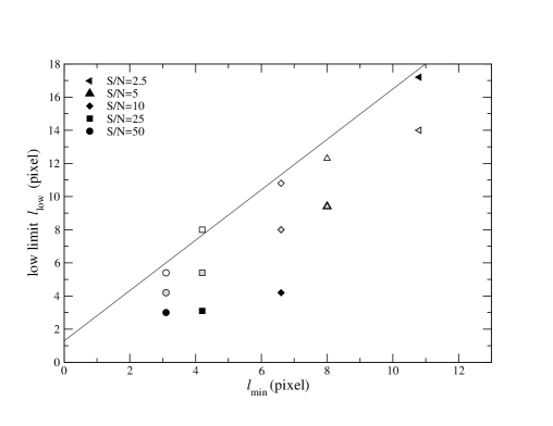
Figure 12: Lower limit for the displacement scale ($l_{\rm low}$) as a function of the $\Delta$-variance minimum scale ($l_{\rm min}$) for $\mathrm{S/N}=2.5,5,10,25,$ and 50, and displacements of $\tau_{i}=4,12,20$ pix (black, gray, and open symbols). An upper limit to the lower scale is described by the solid line: $l_{\rm low}=1.5\,l_{\rm min}+1.5$.

The range $l_{\rm min}\lesssim l\lesssim l_{\rm low}$ thus characterizes scales where the noise does no longer hide the underlying structure – as for scales $l<l_{\rm min}$ – but where it still significantly influences the cross-correlation spectra and the measured displacement vectors.

Figure 13: Measured mean displacement ($\langle{\tau}\rangle$) vs. given displacement ($\tau_{i}$) for $\mathrm{S/N}=\infty$ (circles), $\mathrm{S/N}=25$ (squares), and $\mathrm{S/N}=5$ (triangles). The circles and triangles are displaced by 1 pixel from the identity line (dashed line) for a better visibility. The error bars represent $1\sigma$ error of the mean offset.

To finally verify the reliability of the recovery of the displacement vector within the limits given by Eqs. (27) and (28), we restrict the spectrum of displacement vectors to that range when evaluating the results for 315 pairs of maps covering all combinations of Gaussian widths $\sigma$ = 1, 4, 7, 10, 13, and 16 pix ($l_{\rm p}$ = 4, 16, 28, 40, 52, and 64 pix), input offsets of $\tau_{i,\,y}=0,5,10,15$, and 20 pix, and S/N values of $\infty$, 25, and 5. Fig. 13 shows the measured mean displacement $\langle{\tau}\rangle$ against the given displacement $\tau_{i}$ for the ensembles of 21 pairs having the same offset and noise level. The standard deviation of the derived displacements is very small so that the plotted error bars basically fall within the size of the symbols so that they are hard to be seen.

Overall we find a very good agreement with a minimal scatter, proving the method to work, but a slightly overestimated displacement at $\tau_{i}=0$ pix for high noise ($\mathrm{S/N}=5$, triangle) and a slightly underestimated displacement for the largest offsets at all noise levels, due to the finite map size effects. The deviations fall, however, well below one pixel size. Hence, we conclude that the cutoff of the spectrum of the displacement vectors by low and upper limits allows us to recover accurate offsets, i.e. we can reliably determine the displacement vector between two structures $\@vec{\tau}(l)$ in the full range between $l_{\rm low}$ and $l_{\rm upp}$.

4.2 Structures of fractional Brownian motion

In contrast to the circular Gaussian structures that have a single well-defined prominent scale, maps of the interstellar medium often show a self-similar behavior without individual prominent scales. They can be represented by the fractal structure of fractional Brownian motion maps. They are characterized by a power-law distribution of scales and are periodic by generation in Fourier space. We use a spectral index $\zeta=3$ representing a typical mean value observed in the cold interstellar medium (Falgarone et al. 2007). As for the circular Gaussian structures we evaluate how well the WWCC analysis can detect scales enhanced in one structure compared to the other and the displacement of structures at particular scales within the two maps.

4.2.1 fBm structures displaced on different scales

In real clouds, structures can be offset with respect to each other on different spatial scales. This occurs, e.g., in different velocity channel maps of line observations where the large scale structure is affected by systematic motions but the small scale structure by turbulent motions, in dust emission maps at different wavelengths where local temperature gradients create small scale displacements independent of the possible large scale structure, or in maps of different chemical tracers where incident UV radiation from one direction creates a chemical gradient on scales not mixed by turbulent flows.

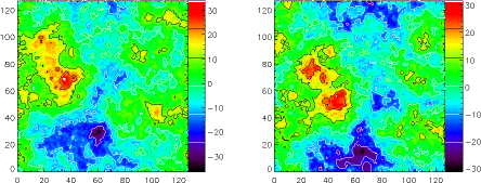
Figure 14: fBm map with $\zeta=3$ (left panel) and the same map after displacing all structures on scales $l\geq 10$ pix by $\tau_{i,x}=10$ pix and $\tau_{i,y}=-15$ pix (right panel). This pair is to mimic an interstellar cloud structure that could be created by the superposition of small scale turbulence and a large scale velocity gradient.

Figure 15: $\Delta$-variance spectra for the maps from Fig. 14.

To test this, we start from an fBm map with a spectral index $\zeta=3$ and $\mathrm{S/N}=\infty$ (Fig. 14, left panel), and shift all structures with scales larger than 10 pixels by $|\@vec{\tau}_{i}|=18$ pix ($\tau_{i,x}=10$ pix and $\tau_{i,y}=-15$ pix) using the Fourier shift theorem (Eq. (25)). The resulting map is shown in Fig. 14 (right panel). The spatial shift of structures does not affect the relative contribution of structures as a function of their size, so that both maps have an identical $\Delta$-variance spectrum, shown in Fig. 15. It is characterized by a perfect power-law with an exponent $\zeta-2=1$, representing the fully self-similar scaling up to the largest scales where the structures are limited by the available map size.

(a) (b)

Figure 16: Results of the WWCC for the pair of maps from Fig. 14: (a) correlation coefficient and (d) displacement vector as a function of scale. $1\sigma$ error bars are given.

Figure 16 shows the results of the WWCC for the comparison of both maps. The correlation coefficient is unity at small scales (because the structures are not offset) and gradually decreases to a minimum at 17–18 pix due to displacement by 18 pix between the structures (Fig. 16 (a)). On large scales the structures are blurred through the wavelet filter to sizes that exceed the displacement amplitude. This leads to monotonic increase of the correlation there. The displacement vector is perfectly recovered for all scales, being zero on scales $l<10$ pix and $\tau_{x}=10$ pix, $\tau_{y}=-15$ pix for larger scales (Fig. 16 (b)).

(a)    (b) (c) (d)

Figure 17: (a) Original fBm map generated with $\mathrm{S/N}=5$ (left) and the same fBm map displaced by $\tau_{i,x}=10$ pix and $\tau_{i,y}=-15$ pix on scales $l\geq 10$ pix (right). (b) $\Delta$-variance of the original and displaced fBm maps, (c) correlation coefficient and (d) displacement vector as a function of scale. $1\sigma$ error bars are presented.

Fig. 17 shows the corresponding results when adding noise to the maps. The noise level of $\mathrm{S/N}=5$ appears as an increased $\Delta$-variance at small scales ($l<8$ pix, panel (b)). It lowers the CC spectrum on scales $l<8$ pix, but has no impact on the measurement of the displacement vector. As the map is filled with structures on all scales, the impact of the noise is much lower here than for the sparsely populated maps inhabiting a single Gaussian circular structure from Sect. 4.1. To ensure that we actually find a smooth transition between the two extreme cases of the single Gaussian circular structure and the fBm map, we also checked the impact of the noise on recovery of the displacement spectrum in case of multiple Gaussian structures. When we compare two maps each having three randomly located Gaussian circular structures with the same characteristics as in Fig. 1 (b) and measure the lower limit for the displacement scale we obtain $l_{\rm low}=5$ pix ($l_{\rm min}=7.7$ pix), i.e. a value that is considerably smaller than that for the single Gaussian structures ($l_{\rm low}=12$ pix, see open upward triangle in Fig. 12). For pairs of maps inhabiting 30 Gaussian structures the impact of the noise further decreases. We obtain $l_{\rm low}=4$ pix ($l_{\rm min}=6.3$ pix) confirming that the noise dominates smaller and smaller scales if the maps are filled with more circular structures. This is in line with a negligible noise impact for the fBm maps filled with structures on all scales (Figs. 16 (b) and 17 (d)).

Identification of correlated structures

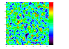
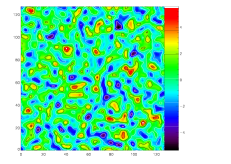
Figure 18: Top left. The fBm map (Fig. 17 (a), left) filtered on scale of 6 pix. Top right. The fBm map displaced on scales $>10$ pix (Fig. 17 (a), right) filtered on scale of 6 pix. Bottom left. The product map generated by multiplying the intensities of the top left and top right fBm maps at each pixel (Eq. (28)).

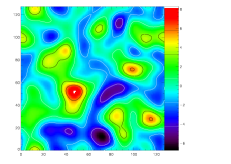
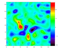
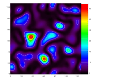
Figure 19: Top left. The fBm map (Fig. 17 (a), left) filtered on scale of 17 pix. Top right. The fBm map displaced on scales $>10$ pix by $\tau_{i,x}=-10$ pix and $\tau_{i,y}=15$ pix (Fig. 17 (a), right) filtered on scale of 17 pix. Bottom left. The product map of two fBm maps (top left and top right). Bottom right. The product map of the top left and top right maps where the latter is reversely shifted by $\tau_{x}=-10$ pix and $\tau_{y}=15$ pix (Eq. (29)).

To understand the nature of the correlations quantified by the WWCC, it is useful to visually inspect the filtered maps for the individual filter scales $l$. In the original maps (Fig. 17 (a)) it is almost impossible to locate individual structures that are correlated between the maps. In the corresponding maps that were wavelet-filtered on the scale of 6 pix (Fig. 18 top), the scale where the CC spectrum showed a peak indicating many correlated structures ($r(l=6\,\,{\rm pix})\approx 0.6$, Fig. 17 (c)), it may be possible to visually identify some prominent structures, but this is extremely difficult due to the noise contribution. An easy identification of correlated structures is however possible if we visualize the integration kernel of the correlation function Eq. (10) for zero offsets $\@vec{\tau}=0$, i.e. show the product of the two maps at each pixel,

$$P(\@vec{x},l)=F(\@vec{x},l)\times G(\@vec{x},l).$$ (29)

In the product map $P(\@vec{x},l)$ (Fig. 18, bottom panel) only relatively strong (positive or negative) features that agree between both maps show up. One can easily recognize individual small “clumps” present in both maps at the same location that can be identified by comparing the product map with the original maps (Fig. 17 (a)).

In Fig. 19 we repeat the experiment for the larger scale of $l=17$ pix where the correlation coefficient is at minimum (Fig. 17 (c)) because the structures are displaced by $\tau_{i,x}=10$ pix and $\tau_{i,y}=-15$ pix ($|\@vec{\tau_{i}}=18$ pix, Fig. 17 (d)). The product map of the filtered maps (Eq. (29), Fig. 19 bottom left panel) shows no structures that can be identified in the individual filtered maps or the original maps in Fig. 17 (a) and the amplitude of the structures in the product map is relatively small. When using, however, the recovered displacement vector at $l=17$ pix to shift the second map back by the measured offset vector $\@vec{\tau}(l)$ and take the product of the shifted map $G(\@vec{x}+\@vec{\tau}(l),l)$ and the first map $F(\@vec{x},l)$ (top right),

$$P(\@vec{x},\@vec{\tau}(l),l)=F(\@vec{x},l)\times G(\@vec{x}+\@vec{\tau}(l),l),$$ (30)

we find that the product map (Fig. 19, bottom right) recovers all of the relatively strong (positive or negative) structures seen in the filtered maps. This allows us to localize individual correlated structures to address their shape and origin, independent of a mutual shift. In Sect. 5 we encounter a pair of observed maps of the G 333 molecular cloud with properties that are very similar to the example considered here. In the observed maps we also find correlated structures with matching locations at small scales, but a global displacements when considering large scale structures.

4.3 Structures of fBm clouds with enhanced scales

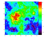
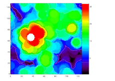
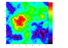
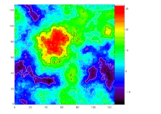
Figure 20: Top left. A pure fBm map generated with $\mathrm{S/N}=\infty$ and spectral index $\zeta=3$. Top right. A pure fBm map filtered with maximum filter of size 15 pix. Bottom left. efBm map which is generated by superimposing the pure fBm structure (top left) and the filtered fBm structure (top right) and for brightness parameter $W=1$. Bottom right. efBm map shifted by $\tau_{i,x}=10$ pix and $\tau_{i,y}=10$ pix.

Pronounced scales in otherwise self-similar clouds may indicate special physical processes acting on those scales, therefore giving access to important characteristics of observed maps. Being able to find and compare those scales in different maps is therefore an essential step in understanding interstellar turbulence. One process producing such enhanced scales is the opacity of partially optically thick lines. They provide a saturated picture for column densities above a specific threshold. To mimic this opacity saturation effect in simulations, we enhance spatial structures in an fBm map $F(\@vec{x})$ by smoothing it with a maximum filter described by

$$\mathcal{M}_{l_{\rm f}}(F(\@vec{x}))=\max{\@vec{x}^{\prime}:|\@vec{x}^{\prime}-\@vec{x}|<l_{\rm f}/2}F(\@vec{x}^{\prime})\;,$$ (31)

where $l_{\rm f}$ is the filter size. The maximum filter enhances the signal on the scale of the filter size and washes out structure on scales less than the filter size. In this way we introduce a prominent scale with size $l_{\rm f}$ into the map. This is demonstrated in Fig. 20. The upper left panel shows the original fBm structure and the upper right panel the result of the convolution with a maximum filter of size $l_{\rm f}=15$ pix. Structures below $l_{\rm f}$ pix are washed there while circles of 15 pix diameter represent the dominant structures now. As the pure opacity effect is always superimposed by additional small scale variations this would give an unrealistic picture. We construct a more realistic picture by combining the original fBm, $F(\@vec{x})$, with the scale-enhanced fBm map, $\mathcal{M}_{l_{\rm f}}(F(\@vec{x}))$:

$$F_{\rm m}(\@vec{x})=WF(\@vec{x})+(2-W)\mathcal{M}_{l_{\rm f}}(F(\@vec{x})),$$ (32)

where we introduce the inverse brightness contrast parameter $W$, ($0<W<2$), characterizing the contribution of the pure fBm in the total map. Then, $2-W$ is the relative brightness of the scale-enhanced map. For values of $W<1$ the enhanced structure is brighter than the pure fBm structure while for $W>1$ it is fainter. This combination should account for the characteristics of the globally self-similar structure and opacity effects. The resulting fBm with enhanced scale (in the following efBm) map is shown in the lower left panel of Fig. 20 for $W=1$.

4.3.1 Recovering the enhanced scale.

Figure 21: $\Delta$-variance spectra of the pure fBm structure and fBm structure filtered at the scale of 15 pix by the maximum filter (full and dotted lines, respectively).

In our numerical experiment we know the size of the maximum filter, but in real observations, one first has to detect and quantify the prominent structures, i.e. the manipulation of the data in our case. Mac Low & Ossenkopf (2000) and O08 have shown that the $\Delta$-variance is an appropriate tool to detect these scales in general astrophysical data sets with irregular boundaries and variable data reliability across the maps. The $\Delta$-variance spectrum measures all prominent scales that are strong enough to create a peak in the spectrum. In a globally self-similar structure like our fBm (or efBm) maps, there is, however, a monotonically increasing $\Delta$-variance spectrum. Figure 21 compares the $\Delta$-variance spectra of the original fBm with the spectrum obtained for the efBm map from Fig. 20. We find no peak in the $\Delta$-variance spectrum – the underlying fBm structure dominates – but information about the filter size, $l_{\rm f}$, is apparently present in the relative drop of structure variation at scales below the filter size. The convolution of the map with the maximum filter of size $l_{\rm f}=15$ pix filters out smaller scale structure. The efBm has less structure on scales $\lesssim 15$ pix, while at scales larger than the size of the maximum filter the $\Delta$-variance of the original fBm is basically recovered in the efBm.

Instead of searching for a peak in the $\Delta$-variance spectrum, we therefore need a new approach to find enhanced scales by looking at the steepening of the $\Delta$-variance spectrum that is visible in Fig. 21. As an auxiliary step, we first look at the pure maximum filter that is described by a filled circle with given diameter $l_{\rm f}$.

Circular structures with constant intensity

The $\Delta$-variance spectrum of a filled circle of diameter $d=20$ pix is shown in Fig. 22 as a full line. The maximum of the $\Delta$-variance falls at $l_{\mathrm{p}}\approx 20$ pix $\approx l_{\rm f}$, as predicted by O08. We verified this for filled circles with $l_{\rm f}=4,8,12,16,20,24,28$ pix.

Figure 22: $\Delta$-variance spectrum $\sigma_{\Delta}^{2}(l)$ of a filled circle of diameter 20 pix (full line) and derivative of the logarithmic $\Delta$-variance spectrum $g(l)$ of the filled circle (dotted line) for $\mathrm{S/N}=\infty$. Vertical lines denote the measured prominent scale of the filled circle at $l_{\mathrm{p}}=21.9$ pix and the critical scale $l_{\mathrm{c}}=10.3$ pix characterizing the peak of the gradient spectrum (Eq. (34)).

To measure the prominent scale even without clear $\Delta$-variance peak, we examine the gradient of the logarithm of the $\Delta$-variance spectrum,

$$g(l)=\frac{\mathrm{d}\log\sigma^{2}_{\Delta}(l)}{\mathrm{d}\log l},$$ (33)

in Fig. 22 (dotted line). The steepening of the $\Delta$-variance spectrum below the prominent scale $l_{\rm f}$ is reflected by a pronounced peak in the gradient spectrum. The root $g=0$ corresponds to the prominent scale $l_{\rm p}$. We define the critical scale as the maximum of the gradient spectrum:

$$l_{\rm c}=\operatorname{arg}\,{\underset{l}{\operatorname{max}}\;}\frac{\mathrm{d}\log\sigma^{2}_{\Delta}(l)}{\mathrm{d}\log l}.$$ (34)

For the filled circle with 20 pixels diameter the measured critical scale is $l_{\rm c}=10.3$ pix, approximately half of the circle’s diameter.

Figure 23: Relation between critical scales and diameter of the circles for $\mathrm{S/N}=\infty,25,$ and 5. The best-fit linear regression line ($l_{\mathrm{c}}\approx 0.52\,l_{\mathrm{p}}$) for $\mathrm{S/N}=\infty$ is shown as solid line.

When computing the $\Delta$-variance gradient spectra for circles of $l_{\rm f}=4,8,12,16,20,24,28$ pix (circles in Fig. 23), we find a linear relation between measured $l_{\mathrm{c}}$ and $l_{\mathrm{f}}$

$$l_{\mathrm{c}}=(0.52\pm 0.02)\,l_{\mathrm{p}}-(0.14\pm 0.36)\approx 0.52\,l_{\mathrm{f}},$$ (35)

shown as solid line in Fig. 23.

Noisy data

To test the robustness of this approach against observational noise, we add different levels of white noise to the circle maps and compute their $\Delta$-variance gradient spectra. In noisy maps, the $\Delta$-variance spectrum at small scales is dominated by noise fluctuations (compare Figs. 4 and 3) so that the critical scale $l_{\rm c}$ is not directly measurable through Eq. (34). To still derive $l_{\rm c}$, one needs to subtract the noise contribution from the $\Delta$-variance spectra of the contaminated circular structures:

$$\sigma_{\Delta}^{2}(l)_{\rm structure}=\sigma_{\Delta}^{2}(l)_{\rm map}-\sigma_{\Delta}^{2}(l)_{\rm noise}.$$ (36)

The corresponding noise spectrum can be obtained by running the $\Delta$-variance analysis on the noise map, obtained e.g. from emission-free channels in an observed spectral line cube. As we construct the noisy map in our numerical simulations by simply adding a noise map to the original map we do not need to extract it separately here.

Using this noise subtraction, we repeated the computation of the gradient peak scale $l_{\mathrm{c}}$ from maps with different circle sizes and noise levels $\mathrm{S/N}=25$ (squares in Fig. 23) and $\mathrm{S/N}=5$ (triangles). We find a very good match to the noise-free results with deviations by up to at most 2 pixels induced by the noise in the data. The regression coefficient ($a=0.54\pm 0.02$) for the noisy maps coincides with one for $\mathrm{S/N}=\infty$ ($a=0.52\pm 0.02$) within the error limits.

For observed maps the determination of the noise $\Delta$-variance $\sigma_{\Delta}^{2}(l)_{\rm noise}$ may, however, be affected by uncertainties that will propagate into the determination of the critical scale $l_{\rm c}$ if the latter falls into the noise-dominated regime. Errors in the noise subtraction will affect the $\Delta$-variance gradient spectrum at scales below the $\Delta$-variance minimum, $l\leq l_{\rm min}$ (see e.g. Fig. 17 (b), $l_{\rm noise\,dominated}\lesssim l_{\rm min}=5$ pix). This puts a lower limit on the scale $l>l_{\rm c}=l_{\rm min}$ that can be reliably measured.

efBm structures

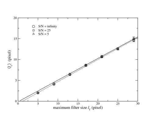
Figure 24: Mean critical scale $l_{\rm c}$ measured for eight fBm maps filtered with the maximum filter of size $l_{\rm f}$ for $\mathrm{S/N}=\infty$, 25 and 5 (circles, squares, and triangles, respectively). 1 $\sigma$ error bars measured in a set of 10 different realizations are superimposed.

In Figure 24 we show the result of the equivalent experiments for the fBm structures with enhanced scales and an inverse brightness contrast $W=1$. The efBms are generated from a fBm map with spectral index $\zeta=3$ which is convolved with the maximum filter of the sizes $l_{\rm f}$ = 5, 9, 13, 17, 21, 25, 29 pix.

For each efBm we use the gradient of the $\Delta$-variance spectrum to measure the critical scale (Eq. (34)). Measured critical scales against maximum-filter sizes are plotted in Fig. 24. The mean critical scale and its uncertainty are estimated from 10 different random realizations of efBms. The circles with error bars represent the noise-free results. The data can be described by a linear relation,

$$\langle l_{\rm c}\rangle=(0.53\pm 0.01)\,l_{\rm f}-(0.61\pm 0.1),$$ (37)

represented by the dashed line in Fig. 24. Within 1 pix accuracy this is identical to the simple approximation without offset from the origin $l_{\mathrm{c}}\approx 0.52\,l_{\mathrm{f}}$ (in agreement with Eq. (35)), obtained for the circular filter, shown as solid line in Fig. 24.

The squares and triangles in Fig. 24 show the measured critical scales for the equivalent noisy maps with $\mathrm{S/N}=25$ and $\mathrm{S/N}=5$ after applying the noise correction from Eq. (36). One can see that the squares and triangles coincide well with circles for $l_{\rm f}>1$ pix and they can be fit by the same linear relation given by Eq. (35) and (37) (see Fig. 24).

To verify that the relation is robust against changes of the efBm spectral index and the inverse brightness contrast $W$ we repeated the experiment for a range of parameters. We vary the fBm spectral index in the range of 2.5 to 3.5 typical for interstellar clouds (Falgarone et al. 2007) and brightness parameters $W=0.1,0.25,0.5,1,1.5,1.75,1.9$. The previous experiment used $\zeta=3$ and $W=1$. For each combination of $\zeta$ and $W$, we recover the critical scales $l_{\rm c}$ for $l_{\rm f}$ = 5, 9, 13, 17, 21, 25, 29 pix and compute the slope $a$ of the $l_{\rm c}-l_{\rm f}$ relation in the range $l_{\rm f}>l_{\rm min}$ pix. To estimate the statistical uncertainty of $a$ we used 10 different random realizations so that the error is composed from the ensemble variation and the imperfection of the linear fit. Figure 25 shows the results for $\mathrm{S/N}=\infty$ and $\mathrm{S/N}=5$.

Figure 25: Measured slope $a$ against inverse brightness contrast $W$ for efBm maps having spectral indexes $\zeta=2.5,3,3.5$ (full, dotted, and dashed lines, respectively). The upper plot shows the result for $\mathrm{S/N}=\infty$, the lower plot for $\mathrm{S/N}=5$. The data points for $\zeta=3$ and 3.5 (squares and triangles) are horizontally displaced by $W=0.02$ and $W=0.04$, respectively, from the $\zeta=2.5$ data points (diamonds) for a better visibility. The error bars represent 1 $\sigma$ variations in the statistical sample.

In case of $\mathrm{S/N}=\infty$ (upper panel), the slope varies in the range between 0.47 and 0.63. It tends to increase with decreasing the spectral index $\zeta$ and increasing inverse brightness contrast $W$. Averaged over the full range of spectral indexes ($\zeta=2.5-3.5$) and inverse brightness contrast parameters ($W=0.1-1.9$) we obtain a mean slope of $\langle a\rangle=0.54\pm 0.03$. When knowing $\zeta$ from the overall slope of the $\Delta$-variance spectrum, the gradient can be even better constrained. For the three spectral indexes we obtain $\langle a\rangle_{\zeta=2.5}=0.57\pm 0.03$, $\langle a\rangle_{\zeta=3}=0.54\pm 0.02$, and $\langle a\rangle_{\zeta=3.5}=0.51\pm 0.01$. These values can be used directly to measure the enhanced scale from the critical scale in the $\Delta$-variance spectrum for large S/N ratios.

In case of the noisy maps (lower panel in Fig. 25), the variation of the slope is only slightly larger for inverse brightness contrasts $W\leq 1.5$ but strongly deviating from the noise-free behaviour for low contrasts of the enhanced structure, i.e. values of $W\geq 1.75$. This is intuitively clear as we see less and less enhanced structure in a map if we reduce its contribution by increasing $W$ to values close to two. If the enhanced structure is strongly diluted ($W>1.5$), the efBm maps appear more like pure fBm maps with only small variations of the gradient of the $\log\sigma^{2}_{\Delta}(l)$ so that the determination of the gradient peak $l_{\rm c}$, becomes very sensitive to the noise contribution. Additional noise makes a reliable detection of the enhanced scale increasingly difficult.

Figure 26: Gradient spectra of fBm maps generated with $\zeta=3$, $\mathrm{S/N}=\infty$, enhanced on scale of $l_{\rm f}=15$ pix and for different inverse brightness contrast parameters $W=0.25,1,1.75$ and 2 (full, dotted, dashed, and dot-dashed lines, respectively). The vertical dashed line indicates the upper limit to the scale where the $\Delta$-variance slope can be measured reliably. Above that scale, the spectrum is strongly affected by boundary effects of the assumed finite map.

The impact of the inverse brightness contrast on the $\Delta$-variance gradient is visualized for the noise-free case ($\mathrm{S/N}=\infty$) in Fig. 26. It shows the gradient spectra of four efBm maps with $\zeta=3$, $l_{\rm f}=15$ pix, and inverse brightness contrasts $W=0.25,1,1.75,2$. The case of $W=2$ (dot-dashed line) represents the pure fBm structure showing the constant gradient $g(l)=\zeta-2=1$ for two-dimensional maps (Stutzki et al. 1998) at scales up to 30 pixels (dashed vertical line in Fig. 26). The drop towards larger scales is due to the impact of the map boundary limiting to size of large structures (O08). This is consistent with our results from Sect. 4.1.4 that only prominent scales up to 64 pixels, i.e. half the map size can be detected. To omit the boundary effects we restrict the analysis to critical scales $l\leq 30$ pix. When adding scale-enhanced structures, $W<2$, we see a growing peak in the gradient spectrum at $l_{\rm c}=8$ pix. It turns sharper if we lower $W$, i.e. the contrast of the peak gradient $g_{\rm max}$ relative to the average gradient $\langle g\rangle$ grows when we increase the contribution of the scale-enhanced structures by lowering the inverse brightness contrast parameter $W$. The contrast of the peak value $g_{\rm max}$ relative to the average $\Delta$-variance gradient $\langle g\rangle$ determines whether $l_{\rm c}$ can be reliably determined, even if uncertainties are added to the spectrum in terms of noise.

Figure 27: $\mathrm{S/N}=5$. Measured maximum gradient versus mean gradient for efBm maps having spectral indexes $\zeta=2.5,3,3.5$ (full line, dotted and dashed lines, respectively) and different inverse brightness contrasts $W=0.1,0.25,0.5,1,1.5,1.75,1.9$. The error bars indicate the standard deviation of the ensemble of 10 different random realizations and seven different enhancement scales. The long-dashed line is the identity representing straight spectra, i.e. $g_{\rm max}=\langle g\rangle$. The dash-dot line represents the lower limit of $g_{\rm max}$ as a function of $\langle g\rangle$ below which the scale of the peak cannot be reliably determined (see Eq. (38)).

In Fig. 27 we show the result of the systematic study of the relation between $g_{\rm max}$ and $\langle g\rangle$ for different values of the spectral index $\zeta$ and the inverse brightness contrast $W$ for $\mathrm{S/N}=5$ where $\langle g\rangle$ is measured between $l_{\rm min}$ and 30 pixels. Averages and error bars are computed for efBms ensembles from ten different random numbers and enhanced on scales of $l_{\rm f}=5,9,13,17,21,25,29$ pix. The series of different inverse brightness contrasts $W$ for the same spectral index $\zeta$ are connected by solid ($\zeta=2.5$), dotted ($\zeta=3.0$), and dashed ($\zeta=3.5$) lines. The long-dashed line indicates the identity, i.e. the behaviour of pure fBms ($W=2$) not showing any maximum in the gradient (dot-dashed line in Fig. 26). Weakly enhanced fBm maps ($W=1.9$) are positioned slightly above the identity. The deviation grows for stronger enhanced fBms, i.e. towards smaller inverse brightness contrasts $W<2$.

As Fig. 25 has shown that for noisy data, the scale of the steepest gradient cannot be reliably determined if the efBm is only weakly enhanced, so that the gradient peak is too shallow, we can translate Fig. 27 into an easily usable criterion for the contrast of $g_{\rm max}$ relative to $\langle g\rangle$ that still allows for a reliable measurement of $a$ and thus $l_{\rm f}$ through $l_{\rm c}$. For $\mathrm{S/N}=5$, points with $W\geq 1.75$ had to be excluded. This corresponds to the area below the dash-dotted line in Fig. 27. It can be described by $g_{\rm max}$ values that fall below

$$g_{\rm max,\,limit}=(1.02\pm 0.01)\langle g\rangle+0.10+3\sigma_{\langle g_{\rm max}\rangle}=1.02\langle g\rangle+0.15$$ (38)

This relation is computed by connecting the data points with $W=1.75$ and adding the 3$\sigma$ error margin of $\sigma_{\langle g_{\rm max}\rangle}=0.017$ of the individual data points. All efBm structures where the enhancement scale cannot be measured reliably due to a too high inverse brightness contrast ($W\gtrsim 1.75$ in Fig. 25 (b)) fall below this relation. For $W\leq 1.5$ critical scales can be reliably recovered for $\mathrm{S/N}=5$. The mean slopes obtained for $\mathrm{S/N}=\infty$ and $\mathrm{S/N}=5$ ($0.54\pm 0.03$ and $0.51\pm 0.04$) agree within the error limits.

Figure 27 can also be used to estimate spectral index and inverse brightness contrast of an efBm by measuring $g_{\rm max}$ and $\langle g\rangle$. For high inverse brightness contrasts $W>0.5$ corresponding to about $g_{\rm max}-\langle g\rangle<0.4$ spectral index and inverse brightness contrast can be uniquely determined, for lower values of $W$ there is an ambiguity in determination of $\zeta$ and $W$ but it is still possible to determine $\zeta$ with an accuracy of about 0.5.

One can generalise the approach of measuring the enhancement scale $l_{\rm f}$ in efBm maps (Eq. (38)) for S/N levels larger than $\mathrm{S/N}=5$. They show different thresholds of the inverse brightness contrast above which $l_{\rm f}$ can not be determined reliably anymore. When lowering the noise, the threshold approaches $W=2$ approximately linearly with the noise level, shifting down the dot-dashed line in Fig. 26 towards the identity line. This corresponds to a change of the constant in Eq. (38) from 0.1 to 0 when S/N increases:

$$g_{\rm max,\,limit}\simeq\langle g\rangle+0.5(\mathrm{S/N})^{-1}+3\sigma_{\langle g_{\rm max}\rangle}.$$ (39)

Global fit

We can adopt the single value $\langle a\rangle=0.52\pm 0.04$ for estimating the enhancement scale,

$$l_{\rm f}=l_{\rm c}/(0.52\pm 0.04)=(1.92\pm 0.15)\,l_{\rm c}.$$ (40)

Even without a priori knowledge of the spectral index of an efBm cloud, one can measure its enhancement scale with accuracy of about $\pm 8$ % if the prominent structure is strong enough to meet the criterion of Eq. (39).

However, Fig. 27 can also be used to estimate spectral index, allowing for a more accurate determination of the slope $a$. When including noise levels from $\mathrm{S/N}=\infty$ to $\mathrm{S/N}=5$ in the fit, we measure the mean slopes $\langle a\rangle_{\zeta=2.5}=0.55\pm 0.04$, $\langle a\rangle_{\zeta=3}=0.53\pm 0.05$, and $\langle a\rangle_{\zeta=3.5}=0.49\pm 0.06$ allowing for a more accurate determination of the enhancement scale $l_{\rm f}$ than through the general equation (40).

Altogether this gives a recipe for the measurement of a pronounced scale in a structure that is globally dominated by self-similarity. After applying the noise correction to the $\Delta$ variance spectrum, the $\Delta$-variance gradient spectrum has to be evaluated to measure the mean gradient $\langle g\rangle$, the peak gradient $g_{\rm max}$, and the location of the peak $l_{\rm c}$. Depending on the noise in the data, the user has to evaluate whether the brightness contrast of the enhanced scale of a cloud is strong enough. If the gradient peak falls above Eq. (39), i.e. $g_{\rm max}>g_{\rm max,\,limit}$, then it is sharp enough to allow for a reliable measurement of its position and one can use the critical scale $l_{\rm c}>l_{\rm min}$ to recover the enhancement scale using the relation $l_{\rm f}=1.92l_{\rm c}$ (Eq. (40)).

4.3.2 Detecting and recovering displacements.

Next, we explore the power of the WWCC to quantify the displacement between different efBm structures through the CC coefficient spectrum and the spectrum of displacement vectors.

In Fig. 28 we show the CC coefficient spectrum when comparing the original fBm and the efBm map without displacement (Fig. 20, top left and bottom left panels). The structures are highly correlated on small and large scales. The scale filtering with $l_{\rm f}=15$ pix produces a small minimum on a scale of about 5 pix due to the reduction of structures below the filter size. Above the filter size both maps turn very similar leading to a cross correlation coefficient close to unity.

Figure 28: Spectrum of the CC coefficient for the original fBm map and efBm map from Fig. 20 (bottom left).

(a) (b)

Figure 29: Results of the WWCC for the original fBm map and the shifted efBm map from Fig. 20 (bottom right): (a) correlation coefficient and (d) displacement vector as a function of scale. $1\sigma$ error bars are given.

Figure 29 (a) shows the result of the WWCC when comparing the fBm map and the efBm map displaced by $\tau_{i}=14.1$ pix ($\tau_{i,x}=10$ pix and $\tau_{i,y}=10$ pix, Fig. 20, top left and bottom right panels). We find a behaviour very similar to that for the displaced Gaussians in Fig. 6. The spectrum of the CC coefficients shows an anti-correlation at small scales with a minimum at $\sim 8$ pix, a steep increase from the minimum to about 30 pix, and a shallower increase at large scales. The spectrum turns to positive CC coefficients at about 14 pix approximately matching the offset amplitude. At larger scales, the correlation becomes stronger as the wavelet filter only measures structures with sizes above the enhancement and offset scale. It is evident that the displacement weakens the correlation on all scales as compared with Fig. 28. The effect is strongest at small scales, i.e. below the offset amplitude. The enhancement of the 15 pix scale in the efBm relative to the original fBm does not affect the recovery of the displacement vector (Fig. 29 (b)). It is accurately measured over all scales $l\lesssim 40$ pix. At larger scales, the finite map size (see Sect. 4.1.3) leads to a small underestimate of the amplitude of the displacement vector by $\sim 5\,\%\leq 1$ pix.

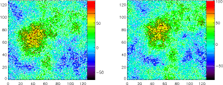
(a)    (b) (c) (d)

Figure 30: WWCC for two efBm maps (shown in (a), maximum-filtered on scales of 15 pix and 5 pix) generated with a $\mathrm{S/N}=5$. The second efBm is shifted by $\tau_{i}=14.1$ pix ($\tau_{i,x}=10$ pix and $\tau_{i,y}=10$ pix). Part (b) shows the $\Delta$-variance spectra of the first map (full line) and the second map (dotted line) with marks of critical scales ($l_{\rm c}=6.4$ pix and $l_{\rm c}=3$ pix, full and dotted vertical lines, respectively) calculated from their noise-corrected spectra, (c) the correlation coefficients and (d) the measured displacement vectors as a function of scale.

To combine all of this, we finally consider a pair of efBm maps with additional noise and an offset by $\tau_{i}=14.1$ pix ($\tau_{i,x}=10$ pix and $\tau_{i,y}=10$ pix, Fig. 30). The first efBm map is generated using a maximum filter of size $l_{\rm f1}=15$ pix, the second efBm map with maximum filter of size $l_{\rm f2}=5$ pix. The noise in both maps gives a $\mathrm{S/N}=5$. The maps are shown in Fig. 30 (a), the $\Delta$-variance spectra in 30 (b), the cross-correlation spectrum in 30 (c), and the spectrum of detected displacement vectors in 30 (d). The effect of the noise is evident in the $\Delta$-variance spectra as an increase of the variance towards small scales. Below $l_{\rm min}\sim 6$ pix the noise dominates, leading to a zero cross-correlation, but it has little effect on the recovery of the displacement vectors. The change of the vector amplitude remains within a 10 % accuracy. Above the noise scale the correlation curve behaves in the same way as in the case of $\mathrm{S/N}=\infty$ (see Fig. 29 (a)). The noise has no effect on $r(l)$ at scales larger than $\approx 6$ pix. The amplitude of the displacement vector is also slightly underestimated on large scales as in the noise-free case. The scale enhancement in both structures has basically no effect on the outcome of the WWCC. It is only visible in the $\Delta$-variance where the two critical scales can be measured as indicated in Fig. 30 (b).

Figure 31: Correlation coefficient as a function of scale for efBm maps filtered with maximum filter of size $l_{\rm f1}=5$ pix and $l_{\rm f2}=15$ pix and offset by 0, 5, 10, 15, and 20 pix (full line, dotted, dashed, dash-dotted, and dash-dot-dot-doted lines, respectively). The dashed vertical lines denote the size of the filters.

To study the quantitative impact of the displacement of the efBm maps on the CC coefficient more quantitatively, we perform the same experiment as for the Gaussians in Fig. 7, using two efBm maps filtered with maximum-filter sizes of $l_{\rm f1}=15$ pix and $l_{\rm f2}=5$ pix displacing them by $\tau_{i,\,y}=0,5,10,15$, and 20 pix relative to each other. The result is shown in Fig. 31. The general behaviour is qualitatively similar to Fig. 7. The shape of the CC coefficient spectrum is regulated by the offset value and ratio between the smaller to the larger filter size, $l_{\rm f2}/l_{\rm f1}$. Without any offset between the maps, we find a strong correlation between structures on all scales. It increases quickly to unity above the scale of the smallest filter size, $l_{\rm f2}=5$. If the structures are offset by 5 pix (dotted line) there is no overlap any more below that scale so that the cross correlation coefficient vanishes. The global shift leads to a lower correlation on all scales, including the largest ones. With increasing the offset (dashed, dashed-dotted, and dash-dot-dot-doted lines) the $r(l)$ curve shifts to larger scales, a scale range of negative values (anticorrelation of filtered structures) appears, and the correlation becomes weaker on all scales. Obviously, the WWCC detects the displacement in the same way for the simple Gaussian structures in Fig.  7 and for close-to self-similar (e)fBm structures.

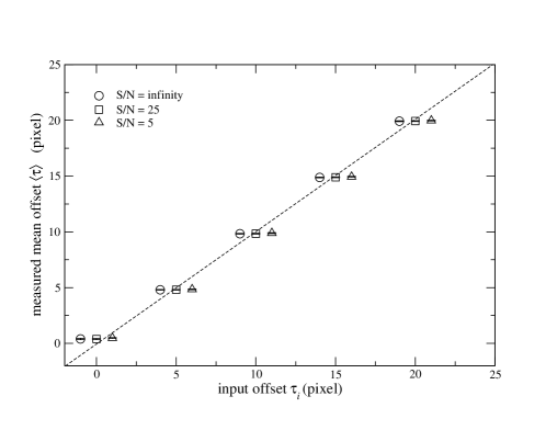
Figure 32: Measured mean displacement ($\langle{\tau}\rangle$) vs. given displacement ($\tau_{i}$) for $\mathrm{S/N}=\infty$, 25, and 5 (filled circles, squares, and filled triangles, respectively). The circles and triangles are displaced by 1 pixel from the identity line (dashed line) for a better visibility. The error bars represent $1\sigma$ variations.

Finally, we test how well the displacement can be recovered for pairs of maps maximum-filtered on different scales. We filter the original fBm map with maximum filters of size $l_{\rm f}=5,9,13,17,21,25,29$ pix to generate seven efBm maps with $\zeta=3.0$ and $W=1$. Combining these seven maps (without repetition) gives 21 pairs of distinct maps. For a given pair of maps, one map is shifted by $\tau_{i}=0,5,10,15,20$ pix, respectively and for each shift we perform the WWCC and recover the displacement ($\tau$; Eq. (21)) for ten random realizations of the fBm. Figure 32 shows the mean recovered displacements separately for $\mathrm{S/N}=\infty,25$ and $5$.

Similar to the case of the Gaussian circular structures (Fig. 13), the mean displacements $\langle{\tau}\rangle$ are recovered with high accuracy for all noise levels and all offsets less than 1/6 of the map size ($\tau_{i}\leq 20$ pix) also for the efBm structures. We also tested the identity between input and recovered displacement for efBm maps generated for all combinations of the spectral index $\zeta=2.5,3$, and 3.5 and the inverse brightness contrast parameter $W=0.5,1,1.5$, (Eq. (32)) and found a perfect agreement for all combinations of $\zeta$ and $W$. The errors of the measured offset depends on the parameter $W$. For large $W$ the offset error slightly increases, however, it remains within the resolution limit $\pm 1$ pix.

5 Application of WWCC to the molecular cloud G 333

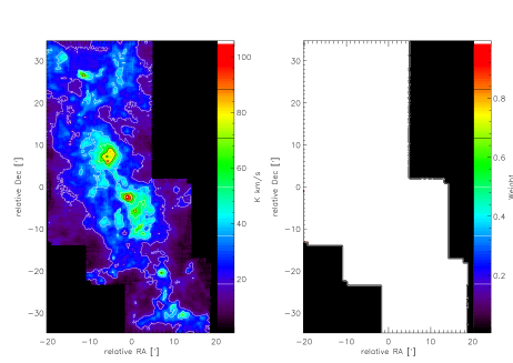
(a) (b) (c)

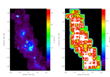
Figure 33: Integrated intensity maps of ¹³CO (a), C¹⁸O (b) and HCN (c) emission lines of the G 333 taken by Lo et al. (2009) (left panels) and significance weights $w$ for the different points in the maps (right panels). White color in the weight map indicates a significance of unity corresponding to a median signal-to-noise ratio of 25 or above. For the ¹³CO map, only pixels close to the map boundary have a lower S/N, i.e. $w<1$.

To test the application of the WWCC to observed maps we selected molecular line maps of the giant molecular cloud G 333 obtained with the Mopra telescope (Lo et al. 2009). Over 20 molecular transitions were mapped and analysed through the Principal Component Analysis (PCA) to investigate spatial correlations among different line transitions and classify molecules into high- and low-density tracers. The PCA quantified the similarity of the different maps for eight significant principal components. Each component can be visualized and the components follow a hierarchy of sizes, but the PCA is not able to clearly identify individual spatial scales at which the similarity of different maps is broken or where gradients between the mapped structures occur. To prove the value of the WWCC in identifying these scales, we selected three of the maps from Lo et al. (2009) that show a different behaviour in the PCA. The maps of ¹³CO 1–0 and C¹⁸O 1–0 show very similar eigenvalues for the first five eigenvectors, indicating a very good correlation at most scales. The map of HCN 1–0 in contrast only shows the same eigenvalue for the first principal component, but a strongly deviating behaviour for basically all other components. Here, we will try to quantify the differences and commonalities seen by the PCA for the three maps in terms of the correlation and displacement between structures in the maps as a function of their spatial scales.

To stay comparable to the results of the PCA, we follow the same procedure in producing the analysed total intensity maps as performed by Lo et al. (2009). The maps were spatially smoothed with an Gaussian of FWHM=45^′′ = 0.75 arcmin and the molecular lines of ¹³CO and C¹⁸O were integrated over the velocity range from $-70$ to $-40$ km s^-1. A wider velocity range from $-80$ to $-30$ km s^-1 was chosen in case of HCN because of visible line wings. The maps are shown in Fig. 33. At the distance of 3.6 kpc of G 333 (Lockman 1979), the resolution of 0.75 arcmin corresponds to 0.79 pc.

In the next step, we need to generate significance maps (weights) for the intensity maps to account for the uncertainty of the information in the individual pixels due to observational noise, stemming from variable sensitivities and finite integration times. Ossenkopf et al. (2008b) proposed to use a saturating linear function of the inverse noise level as weighting function, $w={\rm min}(1,\alpha\times$S/N) with $\alpha$ being an appropriate scaling factor. The choice of the saturation level, i.e. the S/N ratio above which we assume that the distortion of the structural information by noise is negligible, is somewhat arbitrary. Based on our numerical experiments in the previous sections and the inspection of obviously “noisy structures” in the maps, we use a value of S/N=25 here, where we define the signal level as the median of the intensity over the map.

We estimate the noise at each pixel from the emission-free channels in the velocity ranges from $-80$ to $-75$ km s^-1 and $-27$ to $-15$ km s^-1 for ¹³CO and C¹⁸O. For HCN, we use the velocity ranges $-80$ to $-70$ km s^-1 and $-30$ to $-20$ km s^-1. The significance maps are given next to the integrated intensity maps in Fig. 33. Due to the high signal-to-noise ratio of the ¹³CO observations, the S/N=25 limit means that we consider almost all the measured information in the ¹³CO map as reliable, with the exception of a few pixels at the map boundaries that have a lower integration time coverage. For the C¹⁸O and HCN maps, larger regions with low coverage producing some noisy patterns are weighted down by their lower significance in the statistical analysis of the $\Delta$-variance and the WWCC. The significance maps basically represent the coverage of the map in the mosaicing observation with multiple coverages of the individual subfields visible as square areas in the significance maps. Saturated (white) strips and areas in the maps of weights indicate a very good coverage, leading to a low noise so that all details of the lines can be seen. The combination of the mosaicing observations leads to a high significance (low noise) in overlapping areas and a lower significance (higher noise) at the map boundaries. To test the sensitivity of our results on the choice of the saturation limit we varied the limit by a factor two in both directions but found no measurable impact on the $\Delta$-variance spectra and only a small impact on the WWCC on the scale of a few pixels, well within the error bars.

Figure 34: $\Delta$-variance spectra of ¹³CO, C¹⁸O and HCN emission maps (full, dotted and dashed lines, respectively). Prominent scales of the ¹³CO, C¹⁸O and HCN maps are marked by vertical full, dotted, and dashed lines, respectively.

Figure 34 shows the $\Delta$-variance spectra for the integrated intensity maps of ¹³CO, C¹⁸O, and HCN. The C¹⁸O and HCN clouds have a dominant scale size of 7.2 and 10 arcmin (7.5 and 10.5 pc), while the ¹³CO emission has a larger dominant structure with $l_{\rm f}\sim 12$ arcmin (12.5 pc). This matches approximately to the size of the largest structures with more than half of the peak intensity level in the individual maps.

Figure 35: Gradients of the noise-corrected $\Delta$-variance spectra ($g(l)$) of ¹³CO, C¹⁸O and HCN emission maps (full, dotted and dashed lines, respectively). Critical scales of the $\Delta$-variance gradients of ¹³CO, C¹⁸O and HCN are marked by vertical full, dotted, and dashed lines, respectively. The dashed-dotted line represents the gradient spectrum of a pure fBm map ($\zeta=2.5$) convolved with a Gaussian filter of FWHM=0.75 arcmin.

Based on the results from Sect. 4.3.1, we can also estimate the enhanced scale of these maps using the critical scale $l_{\rm c}$ (Eq. (40)) computed from noise-corrected maps (see Appendix A for an example of the noise-correction). The gradient spectra of the noise-corrected $\Delta$-variance are shown in Fig. 35 in comparison to the spectrum obtained for a pure fBm with $\zeta=2.5$ convolved with a Gaussian beam of 0.75 arcmin.

In the overall shape, we find a clear similarity between the spectra from the simulated map and the observed maps. On small scales, there is a peak due to the blurring of smaller structures through the telescope beam with a filter size of 0.75 arcmin as discussed already by Bensch et al. (2001). This dominates the gradient spectra below 2 arcmin. A pure Gaussian beam should provide a monotonous increase towards small scales as seen for the HCN data. The drop of the gradient spectra for the ¹³CO and C¹⁸O at the two smallest lags may be either due to an imperfect noise correction or to a relative surplus of structures at or close to the resolution limit. Therefore, we cannot reliably quantify the structural properties of the maps at scales below 1 arcmin.

Above the scales affected by the beam, we also find a significant difference between the convolved fBm and the observed maps. Instead of the flat spectrum with a drop at scales approaching the map size for the fBm, the observed maps show a clear peak around 5-6 arcmin (5.5 pc) and a quick drop of the gradient towards larger scales, providing the roots that match the prominent scales of 7-12 arcmin (7-12.5 pc) discussed above. The secondary peaks in the gradient spectrum happen on critical scales $\approx 6.3$ arcmin for ¹³CO and HCN and $\approx 4.8$ arcmin for C¹⁸O. Using Eq. (40) this translates into enhancement scales of $\approx 12$ arcmin (¹³CO and HCN, 12.5 pc) and 9 arcmin (C¹⁸O, 9.4 pc), differing from the measured pronounced scales of 12, 10, and 7 arcmin by at most two arcminutes, proving both methods to be approximately consistent.

We can compare the scales found by the $\Delta$-variance analysis with the results from the PCA analysis by Lo et al. (2009). The large-scale distribution of the emission in all lines is traced by the first principal component (their Fig. 14), showing typical structure sizes of 5–10^′, but the PCA only measures to what degree the three maps match to that component. It does not quantify the match or mismatch in terms of a size scale and it does not measure the difference in the dominant structure size for the three maps. The clump analysis also performed by Lo et al. (2009) only finds clumps that are much smaller, with sizes $<2^{\prime}$.

Measurements of $\langle g\rangle$ and $g_{\rm max}$ of a cloud allow to estimate the spectral index by interpolating between $\zeta=2.5,3,$ and 3.5 (Fig. 27). In the inertial range, we expect to find $\langle g\rangle=\zeta-2$. To evaluate $\langle g\rangle$ we are restricted to the range not affected by beam smearing, i.e. to $l>3$ arcmin. We use the plateau before the second peaks (Fig. 35) to estimate the spectral indices of the cloud emission structure as $\zeta_{\rm C^{13}O}=2.8$, $\zeta_{\rm{}^{18}CO}=2.3$, $\zeta_{\rm HCN}=2.5$.

Figure 36: Dependence of the CC coefficient on spatial scale for three pairs of emission maps, ¹³CO and C¹⁸O, ¹³CO and HCN, and C¹⁸O and HCN (full, dotted and dashed lines, respectively).

(a) (b) (c)

Figure 37: Dependence of the displacement vector on spatial scale for three pairs of emission maps, ¹³CO and C¹⁸O (a), ¹³CO and HCN (b), and C¹⁸O and HCN (c).

In Figs. 36 and 37 we show the results of the application of the WWCC to the three pairs of maps ¹³CO and C¹⁸O, ¹³CO and HCN, and C¹⁸O and HCN, in terms of the cross-correlation coefficient spectra and the spectra of displacement vectors. For the pair of ¹³CO and C¹⁸O maps the cross-correlation coefficient shows a strong match ($r(l)\approx 0.85-0.89$) for all scales $>2$ arcmin (Fig. 36). In spite of the apparent differences in the two maps, this confirms the strong similarity of the emission in both molecules, tracing the same conditions of interstellar gas. The difference at small scales is partially due to the noise and partially due to optical depth effects in ¹³CO at the densest spots in the map. The fact that the correlation does not reach unity at larger scales must be basically due to the insufficient excitation of C¹⁸O in low density gas leading to the apparently smaller size of the emitting area and to a lesser degree a result of relatively small systematic displacement. The WWCC result, however proves that this effect is scale-independent (above 2 arcmin), i.e. we find the same amount of thin gas, dark in C¹⁸O but bright in ¹³CO on all spatial scales in the molecular cloud. This is fully in line with the fractal description of molecular clouds.

When comparing the CO isotopes with HCN, however, we find a weaker correlation on all scales and in particular a significant drop of the CC coefficient at the scale below $\approx 7$ arcmin (7 pc). The weakest correlation is found between C¹⁸O and HCN ($r(l>2\,\,{\rm arcmin})\approx 0.7$). The increase of the CC coefficient at 8 arcmin scale is also visible here but less pronounced. This weak correlation contradicts the frequently made assumption that both species are high-density tracers, being sensitive to the same dense gas concentrated in small clumps and cores. As both molecules have very different critical densities our weak correlation at small scales probably reflects different excitation conditions there, i.e. a thermalization of the CO isotopes over larger scales (lower densities) compared to HCN. As all high-density clumps are embedded in lower density envelopes, the correlation is still well above 0.5, but significantly different from unity. Possible physical reasons for kink of the CC curve at the scale of $\approx 7$ arcmin will be discussed in Sect. 5.2.

As the PCA is based on the computation of the cross-correlation matrix (Eq. (10)) we can directly compare our scale dependent cross-correlation coefficients (Eq. (15), Fig. 36) with the global cross correlation coefficients already computed by Lo et al. (2009). They measured coefficients of 0.88, 0.79, and 0.75 for ¹³CO and C¹⁸O, ¹³CO and HCN, and C¹⁸O and HCN maps, respectively, when comparing all pixels of their integrated intensity maps. Lo et al. (2009) did not specify the uncertainty of the coefficients, so that we repeated their computation of the correlation coefficients and obtained errors of about 0.01. When we compare these global CC coefficients with the average of the spectrum of the CC coefficient $r(l)$ over the full range of spatial scales, the scale-averaged CC coefficients are slightly lower ($0.82\pm 0.04$, $0.75\pm 0.05$, and $0.69\pm 0.05$ for ¹³CO and C¹⁸O, ¹³CO and HCN, and C¹⁸O and HCN maps) than the global ones computed without weighting function. The difference is marginally significant and can be due to two effects: the inclusion of the weighting function tends to lower the CC coefficients on large scales by 0.02-0.05, and the small CC coefficients on the noise-dominated scales $\lesssim 2$ arcmin further reduce the average cross correlation coefficient. When restricting ourselves to scales without significant noise distribution, $l>2$ arcmin, we obtain numbers closer to the direct correlation coefficients measured from PCA (0.85, 0.78 and 0.73). This indicates that the global cross-correlation coefficient traces differences in the maps on scales independent from noise quite well, but it does, of course, not deal with a variable reliability of the data and it cannot distinguish between differences on different noise-free scales, such as the varying correlation with HCN below and above 7^′. The WWCC method is capable of recovering the CC coefficients, also measured by the PCA, and, in addition, it allows the analysis of the CC coefficients on scale-by-scale basis.

Figure 37 shows the distribution of measured displacement vectors as a function of scale for the three pairs of maps. There is no displacement between the structures of ¹³CO and C¹⁸O clouds (Fig. 37 (a)) on small scales ($\lesssim 10$ arcmin), while the structure is offset at larger scales with an amplitude of $\sim 1$ arcmin, where all structures in ¹³CO are shifted to the south-west relative to C¹⁸O. If we consider the pairs with HCN, however, we find a much larger offset at large scales (Fig. 37 (b) and (c)). There is a gradual increase of the offset up to $\approx 3.5$ arcmin (HCN relative to ¹³CO) and up to $5$ arcmin (HCN relative to C¹⁸O), where HCN is offset relative to the CO isotopes in south-west direction along the filament.

5.1 Identification of correlated structures

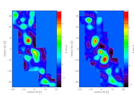
Figure 38: Top panels. Integrated intensity maps of C¹⁸O and HCN emission lines wavelet-filtered on scale of $l=5$ arcmin (left and right panels, respectively). Bottom left. The product map generated by multiplying the two wavelet-filtered maps (top panels).

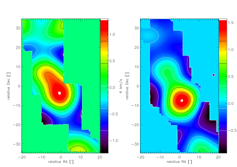
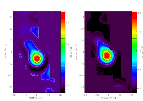
Figure 39: Top panels. Integrated intensity maps of C¹⁸O and HCN emission lines wavelet-filtered on scale of $l=18$ arcmin (left and right panels, respectively). Bottom left. The product map generated by multiplying the two wavelet-filtered maps (top panels). Bottom right. The shifted product map of the top left and top right maps where the latter one is shifted by measured offset in the North-East direction ($\tau_{x}=-2.8$ arcmin and $\tau_{y}=4.5$ arcmin). Note the increase of the signal for the shifted combination compared to the direct product.

To understand the nature of the structures that are actually responsible for the measured shift and correlation we go one step back and look at the individual filtered maps and compare them as for the fBm maps in Sect. 4.2.1. Based on the outcome of the WWCC, we examine here structures with a scale of 5 arcmin, i.e. below the kink in the cross-correlation spectrum at 7 arcmin, and structures at a scale of 18 arcmin, i.e. showing the maximum offset between the maps, for the pair of C¹⁸O and HCN maps.

Figure 38 (top panels) shows the maps wavelet-filtered on the scales of 5 arcmin. The correlation coefficient of the maps at this scale is about $r(l=5^{{}^{\prime}})\approx 0.7$ and the offset between them is small $\tau(l=5^{{}^{\prime}})\approx 0.5^{{}^{\prime}}$. In the figure, we can identify two relatively bright cores in C¹⁸O in the central region of the cloud, one of them also matching a peak in HCN, while the second one breaks up into two knots in HCN. The peak in the filtered HCN map is further offset to the south-west, not having any direct counterpart in C¹⁸O. Multiplication of these maps ($P(\@vec{x},l=5^{{}^{\prime}})$; see Eq. (29), Fig. 38, bottom left) reveals three relatively bright correlated features at the locations of the three knots seen in HCN. In the northern core (relative R.A. $\approx-2^{{}^{\prime}}$, Dec $\approx-2^{{}^{\prime}}$) we find only a small shift of the HCN peak relative to the C¹⁸O peak. In the southern core we find one feature (R.A. $\approx-7^{{}^{\prime}}$, Dec $\approx 7^{{}^{\prime}}$) that is prominent both in C¹⁸O and HCN. The third peak (relative R.A. $\approx 0.3^{{}^{\prime}}$ and Dec $\approx-10^{{}^{\prime}}$) stems from the global peak in the filtered HCN map that has no bright counterpart in the C¹⁸O map, but falls on a relatively faint elongated region there. The matching peaks dominate the cross correlation while the southern knot drives the measured offset. The WWCC result at small scales combines the contribution from all three features. The two matching knots, and in particular the northern core, brightest in C¹⁸O, are very similar in both maps, probably caused by warm and dense core on the scale of $\la 8$ arcmin, have similar emission profiles in both transitions. They create a cross-correlation coefficient of about 0.7 and do not contribute to any measured offset. In the third feature, HCN is clearly offset from the C¹⁸O emission. It hardly contributes to the cross-correlation function, but it produces the measured small global offset.

In Fig. 39 we show the same analysis for the C¹⁸O and HCN maps wavelet-filtered on the scale of 18 arcmin. The WWCC showed a cross-correlation coefficient $r(l=18^{{}^{\prime}})\approx 0.7$ level and a displacement of the HCN structure by $\tau_{x}=2.8$ arcmin and $\tau_{y}=-4.5$ arcmin in south-west direction relative to C¹⁸O (Figs. 36 (dashed line) and 37 (c)). The filtered maps are dominated by a cometary structure with a relatively similar shape, but a clear mutual offset. The simple product map (Fig. 39, bottom left panel) reflects this shape but the displacement between the maps adds a negative arc-like distribution in south-west direction and leads to a low amplitude of the product maps of at maximum 1.8. When accounting for the offset in shifting the HCN map by the measured displacement vector from the WWCC before computing the product map (bottom right panel), the negative arc-like structure disappears, the signal becomes more concentrated in the center of the cometary structure, and the amplitude of the product map grows to 2.1. The weakening of the correlation coefficient on large scales (Fig. 36, dashed line) can be attributed to the offset between C¹⁸O and HCN structures which progressively increases towards large scales (Fig. 37 (c)). It becomes clear that at large scales, the WWCC is dominated by the southern core also seen at small scales. This is systematically offset between HCN and C¹⁸O along the filament and shows a cometary-shape structure at that scale.

5.2 Interpretation

The $\Delta$-variance spectra show the largest difference between the ¹³CO map and the C¹⁸O map while the HCN map exhibits an intermediate behaviour (Fig. 34). The C¹⁸O map has a shallow spectrum with the smallest prominent size, i.e. a relative surplus of small-scale structures relative to the other two maps. This can be seen by eye in Fig. 33. All emission structures and in particular the peaks are smaller than the corresponding structures in the other two tracers. This should be mainly an optical depth effect. Following Lo et al. (2009) most clumps in the source are optically thick in ¹³CO so that one only sees an outer “¹³CO-photosphere” while C¹⁸O traces the full centrally-peaked column density structure. HCN 1–0 has an intermediate optical depth. Consequently, the optical depth effects produce exactly the structure blurring discussed in Sect. 4.3. As a result the $\Delta$-variance spectrum becomes steeper and the pronounced structures appear larger than in the underlying column density profile. The true structure is probably best traced by the C¹⁸O map.

In contrast to this effect, we find a much weaker spatial correlation between the HCN map and the other two maps compared to the mutual correlation between the two CO isotopologue maps. ¹³CO and C¹⁸O emission line maps are strongly correlated above the noise scale. This is explained by the fixed relative abundance and similar excitation conditions, with a critical density of only $2\times 10^{3}$ cm^-3, that lead to a match of the locations of all local features. In that sense, the opacity blurring is only a second-order effect. The small offset of the largest large structures between ¹³CO and C¹⁸O measured in the WWCC indicates that the optical depth is somewhat higher in the south of the C¹⁸O peaks compared to their northern environment, so that the corresponding larger ¹³CO emission pattern is slightly shifted to the south of the C¹⁸O peaks. This means that the column density profile around the cores should have shallower decrease to the south compared to the north.

The globally lower correlation coefficient between HCN and the CO isotopologues indicates a systematically different structure on all scales. We find in particular a clear “kink” towards smaller coefficients at scales below 7 arcmin. At those scales we see in Fig. 38 that the emission of the two main cores in the cloud is very different for HCN and C¹⁸O. In the northern core (-6^′,+6^′) the HCN emission is systematically shifted to the south relative to C¹⁸O and in the southern core (0,-10^′) HCN even peaks at a location south of the C¹⁸O that is not prominent in C¹⁸O at all. This systematic difference could indicate a chemical transition or a density gradient at the measured scale of about 7 pc. The HCN emission peaks in the south of the column density peaks traced by C¹⁸O could stem from an increased HCN abundance, e.g. due to UV illumination (see e.g. Fuente et al. 2005), or from an increased volume density. As HCN 1–0 has a critical density of $10^{6}$ cm^-3, it traces much denser gas than the CO isotopologues. The measured scale is significantly larger than the size of individual clumps in G 333, measured by Wong et al. (2008) and Lo et al. (2009) to fall between about 0.4 and 2 pc, i.e. it must reflect a global process that affects the whole cloud. As such a process continued sequential star-formation was proposed by Nguyen et al. (2015). It would be in line with the compression of gas by newly formed stars. Wong et al. (2008) have observed this process on a scale of 9 arcmin around G 333.6-0.2, the northern region in our map, but that region contributes only to a small degree to the statistics in our whole map. The inclusion of more species that are separately sensitive either to different densities or to chemical changes produced by UV radiation from young stars should allow to distinguish between both effects.

The systematic offset of the HCN structures relative to structures of ¹³CO and C¹⁸O at large scales (Fig. 37 (b) and (c)) can be understood from the emission filtered patterns on large scales shown in Fig. 39. The structures correlated on scales of 18 arcmin have a cometary-like structure oriented in the same north-east direction. The HCN peak at that scale sits at the head of the structure. The measured displacement vector follows the cometary structure due to the shift of the individual HCN peaks towards the south-east of the corresponding C¹⁸O peaks. The combination of this structure and the derived displacement vector indicate a global anisotropy either in the density structure or in the chemical structure. A density structure that is consistent with the observations asks for a statistically higher density in the south-west compared to the north-east. This could be a global feature or a structure where every core shows a low density tail towards the north-east. This would also explain the small shift between ¹³CO and C¹⁸O due to the higher optical depths associated with higher densities in the south-east. A global anisotropy in the abundance structure asks for a preferred direction of the external UV illumination of the cloud. This is not impossible, but there are no independent observational evidences for such a field from the surrounding stars.

Altogether we see that the combination of the $\Delta$-variance analysis and the WWCC allows in principle to distinguish the structural effects of optical depth, excitation, and variable abundance as a function of spatial scale. For a real discrimination between the three effects, however, more data need to be included in the analysis, covering well-defined ranges of critical densities, chemical formation conditions, and optical depths.

6 Summary

We developed the weighted wavelet-based cross correlation (WWCC) to study the correlation and displacement between structural changes in molecular clouds as a function of scale. By inheriting the properties of the $\Delta$-variance analysis from Ossenkopf et al. (2008a) the WWCC method can use a weighting function for each data point in the map to quantify their significance or variable signal-to-noise ratios. The weighting function also allows us to deal with irregular map boundaries and it permits the WWCC analysis through Fast Fourier transform which considerably speeds up the computation.

The method can be applied to observations of interstellar clouds taken in different tracers or at different velocity ranges. The WWCC measures the correlated structural changes between different maps as a function of their spatial scale. Characteristic scales where the behaviour of different tracers starts to match or deviate from each other can be interpreted e.g. as scales of chemical or phase transitions, or driving and dissipation scales in interstellar turbulence.

We performed a series of numerical tests of the WWCC for simulated maps with well-defined spatial properties. It reveals that

• For structures with a well-defined size, the spectrum of cross-correlation (CC) coefficients strongly depends on the displacement between structures and ratio of their prominent scales. The CC spectrum turns negative on small scales if the overlapping area between the two structures becomes small compared to the not overlapping area. The degree and scale range of the anticorrelation depends mainly on the displacement and much less on the size ratio. Beyond the scale of the mutual displacement, the correlation monotonically increases. For structures without dominant scales, the CC spectrum also traces the mutual displacement: it reaches a minimum close to the scale of the offset between the structures. In case of noisy data, the amplitude of the CC spectrum is lowered at small scales, both for correlated and anti-correlated structures.

• The displacement vectors can be reliably recovered at scales dominated by actual structural information, not observational noise. For overall self-similar structures, independent of an enhancement of particular scales, there is always enough structural information on all scales that the displacement vector can be robustly recovered even for relatively low signal to noise levels ($\mathrm{S/N}\geq 5$). In case of individual structures with a fixed size, the lower limit for the reliable measurement of the displacement can be estimated from the minimum of the $\Delta$-variance spectrum, $l_{\rm low}=1.5l_{\rm min}+1.5$ pix and the upper scale is estimated from $l_{\rm upp}=-0.38\,l_{\rm p}+65$ pix, where $l_{\rm p}$ is the prominent scale of the largest structure.

• Mac Low & Ossenkopf (2000) showed that the $\Delta$-variance can be used to measure the scale of individual prominent structures in maps. We extended the $\Delta$-variance analysis to allow for such an identification of enhanced structure scales also in maps that have structure on all scales, but with some scales being slightly more prominent than the rest. By using the logarithmic gradient of the $\Delta$-variance spectrum we can use the scale of the steepest gradient $l_{\rm c}$ to measure the size of the enhanced structure $l_{\rm f}=0.52l_{\rm c}$ as long as the critical scale falls above the noise limit $l_{\rm min}$.

As the results of the WWCC are sometimes non-intuitive, it can be useful to inspect the individual wavelet-filtered maps to understand the origin of a varying cross-correlation and measured displacement vectors in terms of the individual features in the maps that drive the statistical parameters. The product of the maps filtered (and shifted) on a specific scale of interest allows to identify the locations of correlated structures and recognize their shapes.

We analysed molecular line maps (¹³CO, C¹⁸O, and HCN) of the G 333 giant molecular cloud. The $\Delta$-variance spectrum and its gradients (Eq. (40)) allow to measure prominent scales in the maps at 12 arcmin (¹³CO), at 7–9 arcmin (C¹⁸O), and at 10–12 arcmin (HCN). For the changedn turbulent, self-similar structure, covering all spatial scales we can estimate the spectral indices of the power spectrum from the $\Delta$-variance gradient spectrum as $\zeta=2.8$ (¹³CO), $\zeta=2.3$ (C¹⁸O), and $\zeta=2.5$ (HCN). This indicates a gradual difference between the three maps with most small-scale structure and the smallest prominent features in the C¹⁸O data and the dominance of larger structures and a relatively larger prominent structure in ¹³CO. The HCN map shows an intermediate characteristics. All indices are lower than expected from simple Kolmogorov turbulence, but in the typical range observed in molecular line observations of other interstellar clouds (Falgarone et al. 2007).

Application of the WWCC to these molecular line maps shows that:

• ¹³CO and C¹⁸O emission line maps are strongly correlated above the noise scale in spite of their overall very different scaling behaviour. This is expected from a constant relative abundance, similar excitation conditions, and the higher optical depth of ¹³CO. A fixed abundance ratio and identical excitation conditions for both species provide a match of all local features of the map, but a perfect match of all structures is prevented by the larger ¹³CO optical depth. It leads to a suppression of the high density peaks relative to ther lower-density environments in the intensity map so that all emission patches appear somewhat larger in ¹³CO compared to C¹⁸. The measured $1^{\prime}$ offset of the large structures between ¹³CO and C¹⁸O in southern direction indicates that this optical depth effect is slightly anisotropic, due to a shallower density gradient to the south.

• Both the HCN–¹³CO and HCN-C¹⁸O correlations decrease on scales less than 7 arcmin (or 7 pc), where the maps trace different structures. On larger scales, all species trace the overall structure of the molecular cloud resulting in tighter correlations. A chemical differentiation of HCN relative to the CO isotopologues or a very different volume density structure could be the origin of those differences on scales smaller than 7 pc. The offset of the HCN structure relative to structures seen in ¹³CO and C¹⁸O measures the relative shift of the HCN emission to the south along the filament. It may be produced by a higher HCN abundance in the south, due to an overall anisotropic radiation field, or a somewhat higher density in that direction.

Appendix A Recovering the $\Delta$-variance spectrum of an observed map

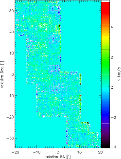
Figure 40: The noise extracted from the C¹⁸O emission line map of the GMC G 333.

To recover the enhancement scale in an efBm-like molecular cloud, we need to correct the measured $\Delta$-variance spectrum for the noise contribution of the observations. Here, we demonstrate the procedure for the G333 C¹⁸O 1-0 map introduced in Sect. 5 (Fig. 33 (b)). In a first step we measure the noise distribution across the map by integrating off-line channels free of emission. To avoid the need for a radiometric correction, we integrate the noise over the same width of a velocity range that is used to integrate the line emission ($\Delta v_{\rm noise}=\Delta v_{\rm line}=30$ km s^-1). In the C¹⁸O data cube this is achieved by integrating the noise over the velocity ranges from $-80$ to $-65$ km s^-1 and from $-35$ to $-20$ km s^-1. The resulting noise map is shown in Fig. 40. In case of ¹³CO and HCN maps, the observed spectra do not contain enough channels free of emission to select the same velocity width for integrating the noise and line emission. To correct for the smaller integration range of the noise channels, $\Delta v_{\rm noise}<\Delta v_{\rm line}$ we have to scale the integrated noise intensity radiometrically by $\sqrt{\Delta v_{\rm line}/\Delta v_{\rm noise}}$.

Figure 41: $\Delta$-variance of the observed C¹⁸O emission line map (dashed line) and the noise emission across the C¹⁸O map in Fig. 40 (dotted line). Their difference represents a pure $\Delta$-variance free of the noise effect (full line). The vertical line denotes the critical scale $l_{\rm c}=0.66$ arcmin at which the pure $\Delta$-variance curve is the steepest. $1\sigma$ error bars are presented.

In the next step, we compute the $\Delta$-variance spectra of the observed C¹⁸O map and the noise map (respective dashed and dotted lines in Fig. 41). A pure $\Delta$-variance spectrum corrected for the noise (full line) is then recovered by subtracting the $\Delta$-variances of the observed C¹⁸O map and the noise. The critical scale can be measured from the gradients in the corrected $\Delta$-variance spectrum (Eq. (34)).

References

- Abergel et al. (1996) Abergel, A.; Bernard, J.-P.; Boulanger, F. et al. 1996, A&A315, L329
- Allan (1996) Allan, D. W., 1996, Proc. IEEE, Vol. 54, No. 2, 221
- Bensch et al. (2001) Bensch, F. and Stutzki, J. and Ossenkopf, V., 2001 A&A, 366, 636
- Deharveng et al. (2010) Deharveng, L., Schuller, F., Anderson, L. D., et al. 2010, A&A, 523, A6
- Falgarone et al. (1998) Falgarone, E., Panis, J.-F., Heithausen, A., et al. 1998, A&A, 331, 669
- Falgarone et al. (2007) Falgarone, E.; Levrier, F.; Hily-Blant, P. 2007, EAS Publ. 23, 73
- Fuente et al. (2005) Fuente, A. and Rizzo, J. R. and Caselli, P. and Bachiller, R. and Henkel, C. 2005, A&A433, 535
- Frick et al. (2001) Frick, P., Beck, R., Berkhuijsen, E. M., & Patrickeyev, I. 2001, MNRAS, 327, 1145
- Glover et al. (2010) Glover, S. C. O. and Federrath, C. and Mac Low, M.-M. et al. 2010, MNRAS, 404, 2
- Goodman et al. (1998) Goodman, A. A.; Barranco, J. A.; Wilner, D. J.; Heyer, M. H. 1998, ApJ504, 223
- Li et al. (2012) Li, P. S., Myers, A., & McKee, C. F. 2012, ApJ, 760, 33
- Liu & Zhang (2006) Liu, X., & Zhang, S.-N. 2006, ApJ, 636, L1
- Lo et al. (2009) Lo, N., Cunningham, M. R., Jones, P. A., et al. 2009, MNRAS, 395, 1021
- Lockman (1979) Lockman F. J., 1979, ApJ, 232, 761
- Mac Low & Ossenkopf (2000) Mac Low M.-M. & Ossenkopf V. 2000, A&A353, 339
- McKee et al. (2010) McKee, C. F., Li, P. S., & Klein, R. I. 2010, ApJ, 720, 1612
- Men’shchikov et al. (2010) Men’shchikov, A., André, P., Didelon, P., et al. 2010, A&A, 518, L103
- Nesme-Ribes et al. (1995) Nesme-Ribes, E., Frick, P., Sokoloff, D., et al. 1995, Academie des Sciences Paris Comptes Rendus Serie B Sciences Physiques, 321, 525
- Nguyen et al. (2015) Nguyen, H., Nguyen Luong, Q., Martin, P. G., et al. 2015, arXiv:1504.02246
- Ossenkopf et al. (2008a) Ossenkopf, V., Krips, M., & Stutzki, J. 2008a, A&A, 485, 917 (O08)
- Ossenkopf et al. (2008b) Ossenkopf, V., Krips, M., & Stutzki, J. 2008b, A&A, 485, 719
- Patrikeev et al. (2006) Patrikeev, I., Fletcher, A., Stepanov, R., et al. 2006, A&A, 458, 441
- Peitgen & Saupe (1988) Peitgen, H. O., & Saupe, D. 1988, The Science of Fractal Images (Springer, New York)
- Roman-Duval et al. (2011) Roman-Duval, J., Federrath, C., Brunt, C., et al. 2011, ApJ, 740, 120
- Roux et al. (2012) Roux, S. G., Koucká Knížová, P., Mošna, Z., & Abry, P. 2012, Journal of Atmospheric and Solar-Terrestrial Physics, 90, 186
- Stutzki et al. (1998) Stutzki, J., Bensch, F., Heithausen, A., Ossenkopf, V., & Zielinsky, M. 1998, A&A, 336, 697
- Stutzki & Guesten (1990) Stutzki, J., & Guesten, R. 1990, ApJ, 356, 513
- Tabatabaei et al. (2013) Tabatabaei, F. S., Berkhuijsen, E. M., Frick, P., Beck, R., & Schinnerer, E. 2013, A&A, 557, A129
- Tabatabaei & Berkhuijsen (2010) Tabatabaei, F. S., & Berkhuijsen, E. M. 2010, A&A, 517, A77
- Vielva et al. (2006) Vielva, P., Martínez-González, E., & Tucci, M. 2006, MNRAS, 365, 891
- Wong et al. (2008) Wong, T., Ladd, E. F., Brisbin, D., et al. 2008, MNRAS, 386, 1069