Group theory of Wannier functions providing the basis for a deeper understanding of magnetism and superconductivity

Abstract

The paper presents the group theory of best localized and symmetry-adapted Wannier functions in a crystal of any given space group G or magnetic group M. Provided that the calculated band structure of the considered material is given and that the symmetry of the Bloch functions at all the points of symmetry in the Brillouin zone is known, the paper details whether or not the Bloch functions of particular energy bands can be unitarily transformed into best localized Wannier functions symmetry-adapted to the space group G, to the magnetic group M, or to a subgroup of G or M. In this context, the paper considers usual as well as spin-dependent Wannier functions, the latter representing the most general definition of Wannier functions. The presented group theory is a review of the theory published by one of the authors in several former papers and is independent of any physical model of magnetism or superconductivity. However, it is suggested to interpret the special symmetry of the best localized Wannier functions in the framework of a nonadiabatic extension of the Heisenberg model, the nonadiabatic Heisenberg model. On the basis of the symmetry of the Wannier functions, this model of strongly correlated localized electrons makes clear predictions whether or not the system can possess superconducting or magnetic eigenstates.

I Introduction

The picture of strongly correlated localized or nearly-localized electrons is the base of a successful theoretical description of both high-temperature superconductivity and magnetism (see, e.g.,  Scalapino (1995); Lechermann et al. (2014); Eberlein and Metzner (2014) and citations given there). In almost all cases the appertaining localized electron states are represented by atomic orbitals that define, for instance, partially filled $s$-, $d$-, or $p$- bands.

Another option would be to represent the localized electron states by best localized and symmetry-adapted Wannier functions. In contrast to atomic functions, Wannier functions situated at adjacent atoms are orthogonal and, hence, electrons occupying (temporarily) adjacent localized states represented by Wannier functions comply with the Pauli principle. In addition, Wannier function form a complete set of basis functions within the considered narrow, partially filled band. Consequently, Wannier functions contain all the physical information about this energy band.

Wannier functions tend to be ignored by the theory of superconductivity and magnetism because we need a closed complex of energy bands [Definition 2.1] for the construction of best localized Wannier functions. Such closed complexes, however, do not exist in the band structures of the metals where all the bands are connected to each other by band degeneracies.

Fortunately, this problem can be solved in a natural way by constructing Wannier functions with the reduced symmetry of a magnetic group or by constructing spin-dependent Wannier functions as shall be details in the present paper. In both cases, interfering band degeneracies are sometimes removed in the band structure with the reduced symmetry.

Against the background of the described characteristics of the Wannier functions, our following two observations should not be too surprising:

1. Materials possessing a magnetic structure with the magnetic group $M$ also possess a closed, narrow and roughly half-filled complex of energy bands in their band structure whose Bloch functions can be unitarily transformed into best localized Wannier functions that are symmetry-adapted to the magnetic group $M$. These energy bands form a “magnetic band”, see Definition 6.2.

2. Both normal and high-temperature superconductors (and only superconductors) possess a closed, narrow and roughly half-filled complex of energy bands in their band structure whose Bloch spinors can be unitarily transformed into best localized spin-dependent Wannier functions that are symmetry-adapted to the (full) space group $G$ of the material. These energy bands form a “superconducting band”, see Definition 7.6.

The first observation (i) was made at the band structures of Cr Krüger (1989a), Fe Krüger (1999), La₂CuO₄ Krüger (2005), YBa₂Cu₃O₆ Krüger (2007), undoped LaFeAsO Krüger and Strunk (2011), and BaFe₂As₂ Krüger and Strunk (2014); the second observation (ii) at the band structures of numerous elemental superconductors Krüger (1978a) and of the (high-temperature) superconductors La₂CuO₄ Krüger (2005), YBa₂Cu₃O₇ Krüger (2010), MgB₂ Krüger (2010), and doped LaFeAsO Krüger and Strunk (2012a). It is particularly important that partly filled superconducting bands cannot be found in those elemental metals (such as Li, Na, K, Rb, Cs, Ca Cu, Ag, and Au) which do not become superconducting Krüger (1978a). An investigation into the band structures of the transition metals in terms of superconducting bands straightforwardly leads to the Matthias rule Krüger (2001a).

Though these two observations are clear, their theoretical interpretation is initially difficult. This is primarily due to the fact that the models of localized electrons developed so far, as, e.g., the familiar Hubbard model Hubbard (1963), are tailored to atomic orbitals that represent the localized states during an electronic hopping motion. Within modern theoretical concepts, the Wannier functions often are nothing but a complete basis in the space spanned by the Bloch functions. Thus, their symmetry is often believed to do not tell anything about the physics of strongly correlated electrons.

In the light of this background, we suggest to interpret the special symmetries of best localized Wannier functions within the nonadiabatic Heisenberg model Krüger (2001b, 2010). This model of strongly correlated localized electrons starts in a consistent way from symmetry-adapted and best localized Wannier functions that represent the localized electron states related to the hopping motion and defines the Hamiltonian $H^{n}$ of the related nonadiabatic system. On the basis of the symmetry of the Wannier functions, the nonadiabatic model makes clear predictions whether or not $H^{n}$ can possess superconducting or magnetic eigenstates Krüger (1978a, 2001c, 1989a); Krüger and Strunk (2014). In this context, the nonadiabatic Heisenberg model no longer uses terms like $s$-, $p$-, or $d$-bands, but only speaks of superconducting or magnetic bands.

In particularly interesting cases, the nonadiabatic Heisenberg model predicts that a small distortion of the lattice or a doping is required for the stability of the superconducting or magnetic state. Thus, in undoped LaFeAsO Krüger and Strunk (2011) and in BaFe₂As₂ Krüger and Strunk (2014) the antiferromagnetic state must be stabilized by an experimentally well established distortion Huang et al. (2008); de la Cruz et al. (2008), while in YBa₂Cu₃O₆ Krüger (2007) it is stable in the undistorted crystal. Superconductivity in LaFeAsO Krüger and Strunk (2011) requires the experimentally confirmed doping de la Cruz et al. (2008); Nomura et al. (2008); Kitao et al. (2008); Nakai et al. (2008). Also the superconducting state in LiFeAs Krüger and Strunk (2012b) should be accompanied by a small distortion of the lattice which, to our knowledge, is experimentally not yet confirmed. Superconductivity in YBa₂Cu₃O₇ Krüger (2010), MgB₂ Krüger (2010) as well as in the transition elements Krüger (1978a) (such as in Nb Krüger (2001c)), on the other hand, does not require any distortion or doping.

In the case of (conventional and high-$T_{c}$ Krüger (1989b)) superconductivity, the nonadiabatic Heisenberg model provides a new mechanism of Cooper pair formation which may be described in terms of constraining forces Krüger (2001c) and spring-mounted Cooper pairs Krüger (2002).

Any application of the nonadiabatic Heisenberg model starts with a determination of the symmetry of best localized (spin-dependent) Wannier functions related to the band structure of the material under consideration. In the following we shall summarize and update the group theory of Wannier functions as published in former papers and give a detailed description how to determine the symmetry of best localized Wannier functions if they exist in the given band structure. Though we shall also define the two terms “magnetic” and “superconducting” bands which are related to the nonadiabatic Heisenberg model, the presented group theory is independent of any physical model of magnetism or superconductivity.

II Usual (spin-independent) Wannier functions

II.1 Definition

Consider a closed complex of $\mu$ energy bands in the band structure of a metal or a semiconductor.

Definition 2.1 (closed).

A complex of energy bands is called closed if the bands are not connected by degeneracies to bands not belonging to the complex.

Definition 2.2 (closed band).

In the following a closed complex of $\mu$ energy bands is referred to as a single closed band consisting of $\mu$ branches.

The metals do not possess closed bands in their band structures. However, closed bands may arise after the activation of a perturbation reducing the symmetry in such a way that interfering band degeneracies are removed. Such a reduction of the symmetry may be caused by a magnetic structure or by a (slight) distortion of the crystal.

Hence, we assume that the Hamiltonian $\mathcal{H}$ of a single electron in the considered material consists of a part $\mathcal{H}_{G}$ with the unperturbed space group $G$ and a perturbation $\mathcal{H}_{H}$ with the space group $H$,

$$\mathcal{H}=\mathcal{H}_{G}+\mathcal{H}_{H},$$ (2.1)

where $H$ is a subgroup of $G$,

$$H\subset G.$$ (2.2)

In general, the considered closed energy band of $\mu$ branches was not closed before the perturbation $\mathcal{H}_{H}$ was activated.

Assume the Bloch functions $\varphi_{\bm{k},q}(\bm{r})$ (labeled by the wave vector $\bm{k}$ and the branch index $q$) as the solutions of the Schrödinger equation of $\mathcal{H}$ to be completely calculated in the first domain of the Brillouin zone.

Definition 2.3 (first domain).

Let be $h$ the order of the point group $H_{0}$ of $H$. Then the Brillouin zone is divided by the planes of symmetry into $h$ domains. An arbitrary chosen domain we call the first domain. This first domain shall comprise the bounding planes, lines and points of symmetry, too.

As in Ref. Krüger (1972a), in the rest of the Brillouin zone the Bloch functions shall be determined by the equation

$$\varphi_{\alpha\bm{k},q}(\bm{r})=P(\{\alpha|\bm{t}_{\alpha}\})\varphi_{\bm{k},q}(\bm{r})\text{ for }\alpha\in H_{0},$$ (2.3)

where $\bm{k}$ lies in the first domain, and in the $\bm{k}$ space outside the Brillouin zone by the equation

$$\varphi_{\bm{k}+\bm{K},q}(\bm{r})=\varphi_{\bm{k},q}(\bm{r}).$$ (2.4)

$\bm{K}$ denotes a vector of the reciprocal lattice and $H_{0}$ stands for the point group of $H$.

Definition 2.4 (symmetry operators).

$P(a)$ denotes the symmetry operator assigned to the space group operation $a=\{\alpha|\bm{t}_{\alpha}\}$ consisting of a point group operation $\alpha$ and the associated translation $\bm{t}_{\alpha}$, acting on a wave function $f(\bm{r})$ according to

$$P(a)f(\bm{r})=f(a^{-1}\bm{r})=f(\alpha^{-1}\bm{r}-\alpha^{-1}\bm{t}_{\alpha}).$$ (2.5)

The Bloch functions $\varphi_{\bm{k},q}(\bm{r})$ of the closed band under observation can be unitarily transformed into Wannier functions

$$w_{i}(\bm{r}-\bm{R}-\bm{\rho}_{i})=\frac{1}{\sqrt{N}}\sum^{BZ}_{\bm{k}}e^{-i\bm{k}(\bm{R}+\bm{\rho}_{i})}\widetilde{\varphi}_{\bm{k},i}(\bm{r})$$ (2.6)

centered at the positions $\bm{R}+\bm{\rho}_{i}$, where the functions

$$\widetilde{\varphi}_{\bm{k},i}(\bm{r})=\sum_{q=1}^{\mu}g_{iq}(\bm{k})\varphi_{\bm{k},q}(\bm{r})$$ (2.7)

are “generalized” Bloch functions Krüger (1972a). The sum in Eq. (2.6) runs over the $N$ vectors $\bm{k}$ of the first Brillouin zone (BZ), the sum in Eq. (2.7) over the $\mu$ branches of the considered band, $\bm{R}$ denote the vectors of the Bravais lattice, and the coefficients $g_{iq}(\bm{k})$ in Eq. (2.7) are the elements of an unitary matrix ${\bf g}(\bm{k})$,

$${\bf g}^{-1}(\bm{k})={\bf g}^{\dagger}(\bm{k}),$$ (2.8)

in order that the Wannier functions are orthonormal,

$$\int w^{*}_{i}(\bm{r}-\bm{R}-\bm{\rho}_{i})w_{i^{\prime}}(\bm{r}-\bm{R}^{\prime}-\bm{\rho}_{i^{\prime}})d\bm{r}=\delta_{\bm{R}\bm{R}^{\prime}}\delta_{ii^{\prime}}.$$ (2.9)

Definition 2.5 (best localized).

The Wannier functions are called best localized if the coefficients $g_{iq}(\bm{k})$ may be chosen in such a way that the generalized Bloch functions $\widetilde{\varphi}_{\bm{k},i}(\bm{r})$ move – for fixed $\bm{r}$ – continuously through to whole $\bm{k}$ space Krüger (1972a).

As it was already shown in Ref. Bouckaert et al. (1936), the Bloch functions $\varphi_{\bm{k},q}(\bm{r})$ as the eigenfunctions of the Hamiltonian $\mathcal{H}$ may be chosen in such a way that they vary continuously as functions of $\bm{k}$ through the first domain and, in particular, approach continuously the boundaries of the first domain. From Eqs. (2.3) and (2.4), however, we cannot conclude that they also cross continuously the boundaries of the domains within the Brillouin zone or at the surface of the Brillouin zone. Fortunately, this problem is solvable by group-theoretical methods Krüger (1972a, b). Theorem 4.1 shall define the condition for best localized and symmetry-adapted [Definition (2.7)] Wannier functions.

II.2 Symmetry-adapted Wannier functions

In Ref. Krüger (1972a) we demanded that symmetry-adapted Wannier functions satisfy the equation

$$w_{i}\big{(}\alpha^{-1}(\bm{r}-\bm{R}-\bm{\rho}_{i})\big{)}=\sum_{j=1}^{\mu}D_{ji}(\alpha)w_{j}(\bm{r}-\bm{R}-\bm{\rho}_{i})$$ (2.10)

for the elements $\alpha$ of the point group $H_{0}$ of $H$, where the $D_{ji}(\alpha)$ are the elements of the matrices

$$\text{\bf D}(\alpha)=\big{[}D_{ij}(\alpha)\big{]}$$ (2.11)

forming a representation $\bm{D}$ of $H_{0}$ which in most cases is reducible. [It should be noted that the sum in Eq. (2.10) runs over $w_{j}(\bm{r}-\bm{R}-\bm{\rho}_{i})$ and not over $w_{j}(\bm{r}-\bm{R}-\bm{\rho}_{j})$.]

Eq. (2.10) defines the symmetry of Wannier functions in general terms, particularly they may be centered at a variety of positions $\bm{\rho}_{i}$ being different from the positions of the atoms. However, in the context of superconducting and magnetic bands we may restrict ourselves to Wannier functions centered at the positions of the atoms.

Thus, we assume

1. that the positions $\bm{\rho}_{i}$ of the Wannier functions in Eq. (2.6) are the positions of atoms,

2. that only atoms of the same sort are considered (although, of course, other atoms may exist), and

3. that there is one Wannier function at each atom.

Under these assumptions Krüger (2001b),

• the Wannier functions may be labeled by the positions of the atoms,

  $$w_{\bm{T}}(\bm{r})\equiv w_{i}(\bm{r}-\bm{R}-\bm{\rho}_{i}),$$ (2.12)

  where

  $$\bm{T}=\bm{R}+\bm{\rho}_{i},$$ (2.13)

• the matrix representatives $\text{\bf D}(\alpha)$ of the representation $\bm{D}$ in Eq. (2.10) have one non-vanishing element $D_{ij}(\alpha)$ with

  $$|D_{ij}(\alpha)|=1$$ (2.14)

  in each row and each column, and

• Eq. (2.10) may be written in the considerably simplified form

  $$P(a)w_{\bm{T}}(\bm{r})=D_{ji}(\alpha)w_{\bm{T}^{\prime}}(\bm{r})\mbox{ for }a\in H$$ (2.15)

  where

  $$\bm{T}^{\prime}=\alpha\bm{T}+\bm{t}_{\alpha}$$ (2.16)

  and the subscripts $i$ and $j$ denote the number of the atoms at position $\bm{T}$ and $\bm{T}^{\prime}$, respectively.

Definition 2.6 (number of the atom).

The subscript $i$ of the vector $\bm{\rho}_{i}$ in Eq. (2.13) defines the number of the atom at position $\bm{T}$.

Definition 2.7 (symmetry-adapted).

We call the Wannier functions symmetry-adapted to $H$ if they satisfy Eq. (2.15).

Theorem 2.1.

The third assumption (iii) shows immediately that the number $\mu$ of the branches of the band under observation equals the number of the considered atoms in the unit cell.

Eqs. (2.15) and (2.16) define the non-vanishing elements and, hence, we may write Eq. (2.14) more precisely,

$$|D_{ji}(\alpha)|=\left\{\begin{array}[]{ll}1&\text{if }\alpha\bm{\rho}_{i}+\bm{t}_{\alpha}=\bm{\rho}_{j}+\bm{R}\\ 0&\text{else,}\\ \end{array}\right.$$ (2.17)

where $\{\alpha|\bm{t}_{\alpha}\}\in H$ and $\bm{R}$ still denotes a lattice vector.

Definition 2.8 (the representation defining the Wannier functions).

In what follows, the representation $\bm{D}$ of $H_{0}$ with the matrix representatives

$${\bf D}(\alpha)=[D_{ij}(\alpha)]$$

defined by Eq. (2.15) shall be shortly referred to as “the representation defining the Wannier functions” and its matrix representatives ${\bf D}(\alpha)$ to as “the matrices defining the Wannier functions”.

Definition 2.9 (unitary generalized permutation matrices).

Since the matrices $\text{\bf D}(\alpha)$ defining the Wannier functions have one non-vanishing element obeying Eq. (2.17) in each row and each column, they are so-called unitary generalized permutation matrices.

III Determination of the representations $\bm{D}$ defining the Wannier functions

In the following Sec IV we shall give a simple condition [Theorem 4.1] for best localized and symmetry-adapted Wannier functions yielding the representations of the Bloch functions at all the points $\bm{k}$ of symmetry in the Brillouin zone. However, in Theorem 4.1 the representations $\bm{D}$ defining the Wannier functions must be known. Hence, first of all we have to determine in this section all the possible representations that may define the Wannier functions. In this context we assume first that all the atoms are connected by symmetry. This restricting assumption shall be abandoned not until in Sec. III.4.

Definition 3.1 (connected by symmetry).

Two atoms at positions $\bm{\rho}_{i}$ and $\bm{\rho}_{j}$ are connected by symmetry if there exists at least one element $a=\{\alpha|\bm{t}_{\alpha}\}$ in the space group $H$ satisfying the equation

$$\alpha\bm{\rho}_{i}+\bm{t}_{\alpha}=\bm{\rho}_{j}+\bm{R},$$ (3.1)

where $\bm{R}$ is a lattice vector.

III.1 General properties of the representatives $\text{\bf D}(\alpha)$ of $\bm{D}$

First consider the diagonal elements

$$d_{i}(\alpha)=D_{ii}(\alpha)$$ (3.2)

of the matrices $\text{\bf D}(\alpha)$ defining the Wannier functions. From Eq. (2.17) we obtain

$$|d_{i}(\alpha)|=\left\{\begin{array}[]{ll}1&\text{if }\alpha\bm{\rho}_{i}+\bm{t}_{\alpha}=\bm{\rho}_{i}+\bm{R}\\ 0&\text{else}\\ \end{array}\right.$$ (3.3)

where $\bm{R}$ denotes a lattice vector. This equation demonstrates that the matrix $\text{\bf D}(\alpha)$ has non-vanishing diagonal elements $d_{i}(\alpha)$ if the space group operation $a=\{\alpha|\bm{t}_{\alpha}\}$ leaves invariant the position $\bm{\rho}_{i}$ of the $i$th atom. These space group operations form a group, namely the group $G_{\bm{\rho}_{i}}$ of the position $\bm{\rho}_{i}$.

Definition 3.2 (group of position).

The group $G_{\bm{\rho}_{i}}$ of the position $\bm{\rho}_{i}$ is defined by

$$a\in G_{\bm{\rho}_{i}}\text{ if }a\in H\text{ and }\alpha\bm{\rho}_{i}+\bm{t}_{\alpha}=\bm{\rho}_{i}+\bm{R}.$$ (3.4)

$G_{0\bm{\rho}_{i}}$ denotes the point group of $G_{\bm{\rho}_{i}}$.

Hence, the non-vanishing diagonal elements $d_{i}(\alpha)$ of the matrices $\text{\bf D}(\alpha)$ form a one-dimensional representation $\bm{d}_{i}$ of the point group $G_{0\bm{\rho}_{i}}$ of $G_{\bm{\rho}_{i}}$. The Wannier functions transform according to

$$P(a)w_{\bm{T}}(\bm{r})=d_{i}(\alpha)w_{\bm{T}+\bm{R}}(\bm{r})\text{ for }\alpha\in G_{0\bm{\rho}_{i}}$$ (3.5)

[cf. Eq. (2.15)] by application of a space group operator $P(a)$ (where $\bm{R}$ still denotes a vector of the Bravais lattice). From Eq. (2.10) we may derive the equivalent equation

$$w_{i}\big{(}\alpha^{-1}(\bm{r}-\bm{R}-\bm{\rho}_{i})\big{)}=d_{i}(\alpha)w_{i}(\bm{r}-\bm{R}-\bm{\rho}_{i})\text{ for }\alpha\in G_{0\bm{\rho}_{i}}$$ (3.6)

or, after shifting the origin of the coordinate system into the center of the function $w_{i}(\bm{r}-\bm{R}-\bm{\rho}_{i})$,

$$\bm{r}^{\prime}=\bm{r}-\bm{R}-\bm{\rho}_{i},$$

we receive an equation

$$w_{i}(\alpha^{-1}\bm{r}^{\prime})=d_{i}(\alpha)w_{i}(\bm{r}^{\prime})\text{ for }\alpha\in G_{0\bm{\rho}_{i}}$$ (3.7)

emphasizing the point-group symmetry of the Wannier function at position $\bm{R}+\bm{\rho}_{i}$.

In constructing the representation $\bm{D}$ defining the Wannier functions we cannot arbitrarily chose the one-dimensional representations ${\bm{d}_{i}}$ of $G_{0\bm{\rho}_{i}}$ because they must be chosen in such a way that the matrix representatives $\text{\bf D}(\alpha)$ form a representation of the point group $H_{0}$, i.e., they must obey the multiplication rule

$$\text{\bf D}(\alpha\beta)=\text{\bf D}(\alpha)\text{\bf D}(\beta)$$ (3.8)

for all the elements $\alpha$ and $\beta$ in $H_{0}$.

In what follows we assume that all the groups $G_{\bm{\rho}_{i}}$ are normal subgroups of $H$. In fact, in all the crystal structures we examined in the past, $G_{\bm{\rho}_{i}}$ was a normal subgroup, be it because it was a subgroup of index 2 or be it because it was the intersection of two subgroups of index 2. Both cases are sufficient for a normal subgroup. We believe that in all physically relevant crystal structures $G_{\bm{\rho}_{i}}$ is a normal subgroup of $H$. If not, the present formalism must be extended for these structures.

When the groups $G_{\bm{\rho}_{i}}$ are normal subgroups of $H$, each of the groups $G_{\bm{\rho}_{i}}$ contains only complete classes of $H$,

$$b^{-1}ab\in G_{\bm{\rho}_{i}}\text{ if }a\in G_{\bm{\rho}_{i}}\text{ and }b\in H.$$ (3.9)

We now show that, as a consequence, all the groups $G_{\bm{\rho}_{i}}$ contain the same space group operations.

Let be $b=\{\beta|\bm{t}_{\beta}\}$ a space group operation of $H$ moving $\rho_{i}$ into $\rho_{j}$,

$$\beta\bm{\rho}_{i}+\bm{t}_{\beta}=\bm{\rho}_{j}+\bm{R},$$

then

$$c=b^{-1}ab$$ (3.10)

is an element of $G_{\bm{\rho}_{i}}$ if $a\in G_{\bm{\rho}_{j}}$. Eq. (3.10) even yields all the elements $c$ of $G_{\bm{\rho}_{i}}$ when $a$ runs throw all the elements of $G_{\bm{\rho}_{j}}$ because we may write Eq. (3.10) in the form

$$bcb^{-1}=a$$

showing that we may determine from any element $c\in G_{\bm{\rho}_{i}}$ an element $a\in G_{\bm{\rho}_{j}}$.

On the other hand, Eq. (3.9) shows that $c$ is an element of $G_{\bm{\rho}_{j}}$, too. When $a$ runs through all the elements of $G_{\bm{\rho}_{j}}$, then also $c$ runs through all the elements of $G_{\bm{\rho}_{j}}$. Consequently, all the groups $G_{\bm{\rho}_{i}}$ as well as all the related point groups $G_{0\bm{\rho}_{i}}$ contain the same elements.

Thus, we may omit the index $i$ and define

Definition 3.3 (group of position).

The group $G_{p}$ and the related point group $G_{0p}$ of the positions of the atoms is defined by

$$G_{p}\equiv G_{\bm{\rho}_{i}}$$ (3.11)

and

$$G_{0p}\equiv G_{0\bm{\rho}_{i}},$$ (3.12)

respectively, where $G_{\bm{\rho}_{i}}$ and $G_{0\bm{\rho}_{i}}$ are given by Definition 3.2.

III.2 Necessary condition for of the representatives $\text{\bf D}(\alpha)$ of $\bm{D}$

The one-dimensional representations $\bm{d}_{i}$ of $G_{0p}$ must be chosen in such a way that the matrices ${\bf D}(\alpha)$ defining the Wannier functions form a representation $\bm{D}$ of the complete point group $H_{0}$. A necessary condition is given by the evident Theorem 3.1.

Theorem 3.1.

If the matrices ${\bf D}(\alpha)$ cannot be completely reduced into the irreducible representations of $H_{0}$, then they do not form a representation of the point group $H_{0}$.

This theorem is necessary, but not sufficient: even if the matrices ${\bf D}(\alpha)$ can be completely reduced into the irreducible representations of $H_{0}$ then they need not form a representation of the point group $H_{0}$ Streitwolf (1967). The complete decomposition of a reducible representation is described, e.g., in Refs. Streitwolf (1967) and Bradley and A.P.Cracknell (1972), in particular, see Eq. (1.3.18) of Ref. Bradley and A.P.Cracknell (1972). Theorem 3.1 leads to three important cases:

• Case (i): If all the representations $\bm{d}_{i}$ are subduced from one-dimensional representations of $H_{0}$, then all the representations $\bm{d}_{i}$ are equal,

  $$\bm{d}_{i}=\bm{d}\quad\text{for all the positions }\bm{\rho}_{i}.$$ (3.13)

  The representation ${\bm{d}}$ may be equal to any one-dimensional representation of $G_{0p}$ subduced from a one-dimensional representation of $H_{0}$.

• Case (ii): If all the representations $\bm{d}_{i}$ are subduced from two-dimensional representations of $H_{0}$, then one half of the representations $\bm{d}_{i}$ is equal to $\bm{d}_{A}$ and the other half is equal to $\bm{d}_{B}$,

  $$\begin{array}[]{lll}\bm{d}_{i}&=&\bm{d}_{A}\quad\text{for one half of the positions }\bm{\rho}_{i}\\ \bm{d}_{i}&=&\bm{d}_{B}\quad\text{for the remaining positions }\bm{\rho}_{i},\\ \end{array}$$ (3.14)

  where $\bm{d}_{A}$ and $\bm{d}_{B}$ are subduced from the same two-dimensional representation of $H_{0}$. In special cases, the two representations $\bm{d}_{A}$ and $\bm{d}_{B}$ may be equal, see below.

• Case (iii): “Mixed” representations $\bm{D}$ consisting of both representations $\bm{d}_{i}$ subduced from one- and two-dimensional representations of $H_{0}$ do not exist.

A further case that the representations $\bm{d}_{i}$ are subduced from three-dimensional representations of $H_{0}$ may occur in crystals of high symmetry but is not considered in this paper.

These results (i) – (iii) follow from the very fact that Eq. (2.15) describes an interchange of the Wannier functions at different positions $\bm{\rho}_{i}$. Such an interchange, however, does not alter the symmetry of the Wannier functions.

III.3 Sufficient condition for of the representatives $\text{\bf D}(\alpha)$ of $\bm{D}$

For $\alpha\in G_{0p}$ the matrices ${\bf D}(\alpha)$ defining the Wannier functions are diagonal, while the remaining matrices ${\bf D}(\alpha)$ [for $\alpha\in H_{0}-G_{0p}$] do not possess any diagonal element. Theorem 3.1 only gives information about the diagonal matrices ${\bf D}(\alpha)$. Hence, this theorem indeed cannot be sufficient because we do not know whether or not the remaining matrices obey the multiplication rule (3.8).

In this section we assume that the matrices ${\bf D}(\alpha)$ already satisfy Theorem 3.1 and examine the conditions under which they actually form a (generally reducible) representation of $H_{0}$. In doing so, we consider separately the two cases (i) and (ii) of the preceding Sec. III.2.

III.3.1 Case (i) of Sec. III.2

No further problems arises when case (i) of Sec. III.2 is realized. In this case, Theorem 3.1 is necessary and sufficient. To justify this assertion, we write down explicitly the non-diagonal elements of the matrices ${\bf D}(\alpha)$.

Let be $\bm{\delta}$ any one-dimensional representation of $H_{0}$ subducing the representation $\bm{d}$ in Eq. (3.13). If we put all the non-vanishing elements of the matrices ${\bf D}(\alpha)$ equal to the elements $\delta(\alpha)$ of $\bm{\delta}$,

$$D_{ji}(\alpha)=\left\{\begin{array}[]{ll}\delta(\alpha)&\text{ if }\alpha\bm{\rho}_{i}+\bm{t}_{\alpha}=\bm{\rho}_{j}+\bm{R}\\ 0&\text{ else,}\\ \end{array}\right.$$ (3.15)

then we receive matrices ${\bf D}(\alpha)$ evidently multiplying as the elements of the representation $\bm{\delta}$ and, consequently, obeying the multiplication rule in Eq. (3.8).

III.3.2 Case (ii) of Sec. III.2

The situation is a little more complicated when case (ii) of Sec. III.2 is realized. Now, the representations $\bm{d}_{A}$ and $\bm{d}_{B}$ in Eq. (3.14) may be distributed across the positions $\bm{\rho}_{i}$ in such a way that the matrices ${\bf D}(\alpha)$ form a representation of $H_{0}$ or do not. Though we always find a special distribution of the $\bm{d}_{A}$ and $\bm{d}_{B}$ yielding matrices ${\bf D}(\alpha)$ actually forming a representation of $H_{0}$, we have to rule out those distributions not leading to a representation of $H_{0}$, because in the following [in Eqs. (4.1), (6.10), and (7.42)] we need the matrices ${\bf D}(\alpha)$ explicitly.

Let be $\bm{\Delta}$ [with the matrix representatives $\bm{\Delta}(\alpha)$] a two-dimensional representation of $H_{0}$ subducing the two representations $\bm{d}_{A}$ and $\bm{d}_{B}$ of $G_{0p}$. The matrix representatives $\bm{\Delta}(\alpha)$ may be determined, e.g., from Table 5.1 of Ref. Bradley and A.P.Cracknell (1972).

As a first step, $\bm{\Delta}$ must be unitarily transformed (by a matrix Q) in such a way that the matrices $\bm{\Delta}(\alpha)$ are diagonal for $\alpha\in G_{0p}$,

$$\overline{\bm{\Delta}}(\alpha)={\bf Q}^{-1}{\bm{\Delta}}(\alpha){\bf Q}\quad=\text{ diagonal for }\alpha\in G_{0p}.$$ (3.16)

Now consider a certain distribution of the representations $\bm{d}_{A}$ and $\bm{d}_{B}$ across the positions $\bm{\rho}_{i}$. Then we may determine the elements of the matrices ${\bf D}(\alpha)$, if they exist, be means of the formula

$$\begin{array}[]{l}\text{if}\quad\alpha\bm{\rho}_{i}+\bm{t}_{\alpha}=\bm{\rho}_{j}+\bm{R}\\ \\ D_{ji}(\alpha)=\left\{\begin{array}[]{lll}\overline{\Delta}_{12}(\alpha)&\text{ if }\bm{d}_{j}=\bm{d}_{A}&\text{and }\bm{d}_{i}=\bm{d}_{B},\\ \\ \overline{\Delta}_{21}(\alpha)&\text{ if }\bm{d}_{j}=\bm{d}_{B}&\text{and }\bm{d}_{i}=\bm{d}_{A},\\ \\ \overline{\Delta}_{11}(\alpha)&\text{ if }\bm{d}_{j}=\bm{d}_{A}&\text{and }\bm{d}_{i}=\bm{d}_{A},\\ \\ \overline{\Delta}_{22}(\alpha)&\text{ if }\bm{d}_{j}=\bm{d}_{B}&\text{and }\bm{d}_{i}=\bm{d}_{B},\\ \end{array}\right.\\ \\ \text{else}\\ \\ D_{ji}(\alpha)=0,\\ \\ \end{array}$$ (3.17)

where the $\overline{\Delta}_{ij}(\alpha)$ denote the elements of $\overline{\bm{\Delta}}(\alpha)$.

It turns out that in each case the matrices determined by Eq. (3.17) satisfy the multiplication rule in Eq. (3.8) if Eq. (3.17) produces for each space group operation $a\in H$ an unitary generalized permutation matrix ${\bf D}(\alpha)$. This may be understood because Eq. (3.17) defines the complex numbers $D_{ji}(\alpha)$ in such a way that the Wannier functions transform in Eq. (2.15) in an unequivocal manner like the basis functions for $\overline{\bm{\Delta}}$. With “like” the basis functions we want to express that by application of any space group operator $P(\{\alpha|\bm{t}_{\alpha}\})$ they are multiplied in Eq. (2.15) by the same complex number $\overline{\Delta}_{ij}(\alpha)$ as the basis functions for $\overline{\bm{\Delta}}$. The Wannier functions would indeed be basis functions for $\overline{\bm{\Delta}}$ if they would not be moved from one position $\bm{\rho}_{i}$ to another by some space group operations. Hence, we may expect that the matrices ${\bf D}(\alpha)$ satisfy the multiplication rule in Eq. (3.8) just as the matrices $\overline{\bm{\Delta}}(\alpha)$ do. Nevertheless, the multiplication rule should be verified numerically in any case.

When using this Eq. (3.17) a little complication arises if the group of position $G_{0p}$ contains so few elements that the two one-dimensional representations $\bm{d}_{A}$ and $\bm{d}_{B}$ subduced from $\overline{\bm{\Delta}}$ are equal. Thus, in this case we have no problem with the distribution of $\bm{d}_{A}$ and $\bm{d}_{B}$ across the positions $\bm{\rho}_{i}$. Theorem 3.1 is necessary and sufficient and we may directly solve Eq. (4.1) of Theorem 4.1.

However, when in Sec. VI or in Sec. VII.3 we will consider magnetic groups, we need all the representatives ${\bf D}(\alpha)$ of the representation $\bm{D}$ explicitly. Fortunately, also when the representations $\bm{d}_{A}$ and $\bm{d}_{B}$ are equal, Eq. (3.17) is applicable: in this case their exists at least one diagonal matrix representative $\overline{\bm{\Delta}}(\gamma)$ of $\overline{\bm{\Delta}}$ with vanishing trace and $\gamma\notin G_{0p}$. We may define pairs

$$(\bm{\rho}_{a},\bm{\rho}_{b}),\quad(\bm{\rho}_{c},\bm{\rho}_{d}),\quad\ldots$$ (3.18)

of positions $\rho_{i}$ where the positions in each pair are connected by the space group operation $\{\gamma|\bm{t}_{\gamma}\}$. In the simplest case, we receive two pairs. Then in Eq. (3.17) we may identify the two representations at $\bm{\rho}_{a}$ and $\bm{\rho}_{b}$ by $\bm{d}_{A}$ and the representations at the other two positions $\bm{\rho}_{c}$ and $\bm{\rho}_{d}$ by $\bm{d}_{B}$. If we find four pairs of positions, we may look for a second matrix representative $\overline{\bm{\Delta}}(\gamma^{\prime})$ in $\overline{\bm{\Delta}}$ with vanishing trace and $\gamma^{\prime}\notin G_{0p}$. Then we may repeat the above procedure and receive again four pairs of positions. Now we associate the two representations $\bm{d}_{A}$ and $\bm{d}_{B}$ to the positions $\bm{\rho}_{i}$ under the provision that always positions of the same pair are associated with the same representation $\bm{d}_{A}$ or $\bm{d}_{B}$.

Finally, it should be mentioned that the elements of the non-diagonal matrices ${\bf D}(\alpha)$ are not fully fixed (as already remarked in Ref. Krüger (1972b)): In Eq. (3.15) we may use the elements $\delta(\alpha)$ of any one-dimensional representation $\bm{\delta}$ subducing the representation $\bm{d}$. We receive in each case the same diagonal, but different non-diagonal matrices nevertheless satisfying the multiplication rule (3.8). Analogously, in Eq. (3.17) we may determine the matrices ${\bf D}(\alpha)$ by means of any two-dimensional representation $\overline{\bm{\Delta}}$ subducing $\bm{d}_{A}$ and $\bm{d}_{B}$.

In the following Theorem 3.2 we summarize our results in the present Sec. III.3.

Theorem 3.2.

The Wannier function $w_{i}(\bm{r}-\bm{R}-\bm{\rho}_{i})$ at the position $\bm{\rho}_{i}$ is basis function for a one-dimensional representation $\bm{d}_{i}$ of the “point group of position” $G_{0p}\subset H_{0}$ [Definition 3.3], cf. Eq. (3.7). The representations $\bm{d}_{i}$ fix the (generally reducible) representation $\bm{D}$ of $H_{0}$ defining the Wannier functions [Definition 2.8]. The matrix representatives ${\bf D}(\alpha)$ of $\bm{D}$ are unitary generalized permutation matrices. We distinguish between two cases (i) and (ii).

Case (i): If the representations $\bm{d}_{i}$ are subduced from one-dimensional representations of the point group $H_{0}$, then all the Wannier functions of the band under observation are basis functions for the same representation $\bm{d}$ which may be any one-dimensional representation of $G_{0p}$ subduced from a one-dimensional representation of $H_{0}$. The representation $\bm{D}$ exists always, its matrix representatives ${\bf D}(\alpha)$ may be calculated by Eq. (3.15).

Case (ii): If the representations $\bm{d}_{i}$ are subduced from two-dimensional representations of the point group $H_{0}$, then the Wannier functions are basis functions for the two one-dimensional representations $\bm{d}_{A}$ and $\bm{d}_{B}$ of $G_{0p}$ subduced from the same two-dimensional representation of $H_{0}$. One half of the Wannier functions is basis function for $\bm{d}_{A}$ and the other half for $\bm{d}_{B}$. In special cases, the representations $\bm{d}_{A}$ and $\bm{d}_{B}$ may be equal, see above. The representation $\bm{D}$ exists for a given distribution of the representations $\bm{d}_{A}$ and $\bm{d}_{B}$ across the positions $\bm{\rho}_{i}$ if Eq. (3.17) yields unitary generalized permutation matrices ${\bf D}(\alpha)$ satisfying the multiplication rule in Eq. (3.8).

A third case with representations $\bm{d}_{i}$ subduced from one-dimensional as well as from two-dimensional representations of $H_{0}$ does not exist.

III.4 Not all the atoms are connected by symmetry

If not all the atoms at the positions $\bm{\rho}_{i}$ are connected by symmetry [Definition 3.1], the representation $\bm{D}$ defining the Wannier functions consists of representatives $\text{\bf D}(\alpha)$ which may be written in block-diagonal form

$${\bf D}(\alpha)=\left(\begin{array}[]{ccc}\left(\begin{array}[]{c}\\ \textnormal{block 1}\\ \\ \end{array}\right)&0&\cdots\\ 0&\left(\begin{array}[]{c}\\ \textnormal{block 2}\\ \\ \end{array}\right)&\cdots\\ \vdots&\vdots\\ \end{array}\right),$$ (3.19)

where each block comprises the matrix elements $D_{ij}(\alpha)$ belonging to positions connected by symmetry. Otherwise, when the matrices ${\bf D}(\alpha)$ would not possess block-diagonal form, Eq. (2.10) would falsely connect atomic positions that are not at all connected by symmetry. As a consequence of the block-diagonal form, the representation $\bm{D}$ is the direct sum over representations $\bm{D}^{q}$ related to the individual blocks,

$$\bm{D} = \bm{D}^{1}\oplus\bm{D}^{2}\oplus\ldots$$ (3.20)

$$= \sum_{q}\bm{D}^{q}.$$

We may summarize as follows.

Theorem 3.3.

Each block $\bm{D}^{q}$ in Eq. (3.20) forms its own representation of $H_{0}$ and, hence, must comply separately and independently with the criteria given in Theorem 3.2.

The groups of position $G_{p}$ belonging to different blocks may (but need not) be different. However, we assume that the sum in Eq. (3.20) consists only of blocks with coinciding groups of position. If this is not true in special cases, the number $\mu$ of the atoms in Eq. (2.7) must be reduced until the groups of position coincide in the sum in Eq. (3.20). Briefly speaking, in such a (probably rare) case atoms of the same sort must be treated like different atoms.

IV Condition for best localized symmetry-adapted Wannier functions

Remember that we consider a closed energy band of $\mu$ branches and let be given a representation $\bm{D}$ defining the Wannier functions which was determined according to Theorems 3.2 and 3.3. Then we may give a simple condition for best localized symmetry-adapted Wannier functions based on the theory of Wannier functions published in Refs. Krüger (1972a) and Krüger (1972b).

Theorem 4.1.

Let be $\bm{k}$ a point of symmetry in the first domain of the Brillouin zone for the considered material and let be $H_{\bm{k}}\subset H$ the little group of $\bm{k}$ in Herrings sense. That means, $H_{\bm{k}}$ is the FINITE group denoted in Ref. Bradley and A.P.Cracknell (1972) by ${}^{H}\!G^{\bm{k}}$ (and listed for all the space groups in Table 5.7 ibidem). Furthermore, let be $\bm{D}_{\bm{k}}$ the $\mu$-dimensional representation of $H_{\bm{k}}$ whose basis functions are the $\mu$ Bloch functions $\varphi_{\bm{k},q}(\bm{r})$ with wave vector $\bm{k}$, and $\chi_{\bm{k}}(a)$ (with $a\in H_{\bm{k}}$) the character of $\bm{D}_{\bm{k}}$. $\bm{D}_{\bm{k}}$ either is irreducible or the direct sum over small irreducible representations of $H_{\bm{k}}$.

We may choose the coefficients $g_{iq}(\bm{k})$ in Eq. (2.7) in such a way that the Wannier functions are best localized [Definition 2.1] and symmetry-adapted to $H$ [Definition 2.7] if the character $\chi_{\bm{k}}(a)$ of $\bm{D}_{\bm{k}}$ satisfies at each point $\bm{k}$ of symmetry in the first domain of the Brillouin zone the equation

$$\chi_{\bm{k}}(a)=e^{-i\alpha\bm{k}\cdot\bm{t}_{\alpha}}~{}\sum_{i=1}^{\mu}n_{i}(a)e^{-i\bm{\rho}_{i}\cdot(\bm{k}-\alpha\bm{k})}\text{ for }a\in H_{\bm{k}},$$ (4.1)

where $a=\{\alpha|\bm{t}_{\alpha}\}$ and

$$n_{i}(a)=\left\{\begin{array}[]{ll}d_{i}(\alpha)&\text{ if }\quad\alpha\in G_{0p}\\ 0&\text{ else.}\\ \end{array}\right.$$ (4.2)

The complex numbers $d_{i}(\alpha)$ stand for the elements of the one-dimensional representations $\bm{d}_{i}$ of $G_{0p}$ fixing the given $\mu$-dimensional representation $\bm{D}$ defining the Wanner functions.

Definition 4.1 (point of symmetry).

The term “point of symmetry” we use as defined in Ref. Bradley and A.P.Cracknell (1972): $\bm{k}$ is a point of symmetry if there exists a neighborhood of $\bm{k}$ in which no point except $\bm{k}$ has the symmetry group $H_{\bm{k}}$.

Thus, a point $\bm{k}$ of symmetry has a higher symmetry than all surrounding points.

We add a few comments on Theorem 4.1.

• In Eq. (4.2) we write $n_{i}(a)$ rather than $n_{i}(\alpha)$ because the group $G_{0p}$ depends on $a=\{\alpha|\bm{t}_{\alpha}\}$.

• The representation $\bm{D}$ defining the Wannier functions is equivalent to the representation $\bm{D}_{\bm{0}}$, i.e., to the representation $\bm{D}_{\bm{k}}$ for $\bm{k}=\bm{0}$, see Eq. (5.10).

• In the majority of cases all the representations $\bm{d}_{i}$ in Eq. (4.2) are equal. The only exceptions arises when

  1. not all the positions $\bm{\rho}_{i}$ are connected by symmetry or

  2. the one-dimensional representations $\bm{d}_{i}$ of $G_{0p}$ are subduced from a higher-dimensional representation of $H_{0}$.

• A basic form of Theorem 4.1 was published first in Eq. (23) of Ref. Krüger (2005) and used in several former papers. Eq. (23) of Ref. Krüger (2005) yields the same results as Theorem 4.1

  1. if all the $\bm{\rho}_{i}$ are connected by symmetry and

  2. if all the representations $\bm{d}_{i}$ of $G_{0p}$ are subduced from one-dimensional representations of $H_{0}$.

  These two conditions were satisfied in our former papers.

• The irreducible representations of the Bloch functions of the considered band at the points $\bm{k}$ of symmetry may be determined from the representations $\bm{D}_{\bm{k}}$ as follows:

Theorem 4.2.

Let $H_{\bm{k}}$ possess $r$ irreducible representations with the characters $\chi_{\bm{k},m}(a)\quad(1\leq m\leq r)$ and assume that $\bm{D}_{\bm{k}}$ contains the $m$th irreducible representation, say, $c_{m}$ times. Then the numbers $c_{m}$ may be calculated by means of Eq. (1.3.18) of Ref. Bradley and A.P.Cracknell (1972),

$$c_{m}=\frac{1}{|H_{\bm{k}}|}\sum^{H_{\bm{k}}}_{a}\chi_{\bm{k},m}(a)\chi^{*}_{\bm{k}}(a),$$ (4.3)

where $\chi_{\bm{k}}(a)$ denotes the character of $\bm{D}_{\bm{k}}$ as determined by Eq. (4.1) and the sum runs over the $|H_{\bm{k}}|$ elements $a$ of $H_{\bm{k}}$. Remember [Theorem 4.1] that $H_{\bm{k}}$ is a finite group.

V Proof of Theorem 4.1

The existence of best localized symmetry-adapted Wannier functions is defined in Satz 4 of Ref. Krüger (1972a): such Wannier functions exist in a given closed energy band of $\mu$ branches if Eqs. (4.28) and (4.17) of Ref. Krüger (1972a) are satisfied. We show in this section that the fundamental Theorem 4.1 complies with these two equations if the Wannier functions meet the assumptions (i) – (iii) in Sec. II.2.

V.1 Equation (4.28) of Ref. Krüger (1972a)

As a first step consider Eq. (4.28) of Ref. Krüger (1972a) stating that best localized and symmetry-adapted Wannier functions may exist only if two representations $\widehat{\bm{D}}_{\bm{k}^{\prime}_{\Sigma R}}$ and $\bm{D}_{\bm{k}^{\prime}_{\Sigma R}}$ are equivalent,

$$\widehat{\bm{D}}_{\bm{k}}\text{ equivalent to }\bm{D}_{\bm{k}},$$ (5.1)

where we have abbreviated $\bm{k}^{\prime}_{\Sigma R}$ by $\bm{k}$ denoting a point of symmetry lying in the first domain of the Brillouin zone. Consequently, our first task will be to determine the character of $\widehat{\bm{D}}_{\bm{k}}$ as well as of $\bm{D}_{\bm{k}}$,

The representation $\bm{D}_{\bm{k}}$ as defined in Theorem 4.1 is the direct sum of the representations of the Bloch functions of the considered band at point $\bm{k}$. The character $\chi_{\bm{k}}(a)$ of the representation $\bm{D}_{\bm{k}}$ is simply given by

$$\chi_{\bm{k}}(a)=\text{trace\ \bf D}_{\bm{k}}(a)$$ (5.2)

where the matrices $\text{\bf D}_{\bm{k}}(a)$ are the matrix representatives of $\bm{D}_{\bm{k}}$.

The matrix representatives $\widehat{\text{\bf D}}_{\bm{k}}(a)$ of $\widehat{\bm{D}}_{\bm{k}}$ are defined in Eq. (4.26) of Ref. Krüger (1972a),

$$\widehat{\text{\bf D}}_{\bm{k}}(a)=\text{\bf S}^{*}(\bm{K}_{\alpha})\text{\bf D}_{\bm{0}}(\alpha)e^{-i\alpha\bm{k}\bm{t}_{\alpha}}$$ (5.3)

where

$$\bm{K}_{\alpha}=\bm{k}-\alpha\bm{k}$$ (5.4)

is a vector of the reciprocal lattice. Again we have abbreviated $\bm{k}^{\prime}_{SR}$ by $\bm{k}$ denoting a point of symmetry. The matrices $\text{\bf S}(\bm{K})$ as defined in Eq. (4.13) of Ref. Krüger (1972a) are responsible for a continuous transition of the generalized Bloch functions between neighboring Brillouin zones. The matrices ${\bf D}_{\bm{0}}(\alpha)$ are the matrix representatives of the representation $\bm{D}_{\bm{k}}$ for $\bm{k}=\bm{0}$ as defined in Theorem 4.1. $\bm{D}_{\bm{0}}$ is the direct sum of the irreducible representations of the Bloch functions of the considered band at point $\Gamma$.

The traces of the matrices $\widehat{\text{\bf D}}_{\bm{k}}(a)$ can be determined by transforming Eq. (5.3) with the complex conjugate of the matrix M defined by Eq. (2.1) of Ref. Krüger (1972b),

$${\bf M}^{*}\widehat{\text{\bf D}}_{\bm{k}}(a){\bf M}^{*-1} = {\bf M}^{*}{\bf S}^{*}(\bm{K}_{\alpha}){\bf M}^{*-1}\times$$

$${\bf M}^{*}{\bf D}_{\bm{0}}(\alpha){\bf M}^{*-1}\times$$

$$e^{-i\alpha\bm{k\cdot t_{\alpha}}},$$

where $a=\{\alpha|\bm{t}_{\alpha}\}$ still denotes an element of the space group $H$. By definition, the matrix M diagonalizes the matrices $\text{\bf S}(\bm{K})$ which is possible since all the $\text{\bf S}(\bm{K})$ commute. Thus, the first factor $\text{\bf M}^{*}\text{\bf S}^{*}(\bm{K}_{\alpha})\text{\bf M}^{*-1}$ in Eq. (V.1) is the diagonal matrix

$$\overline{\text{\bf S}}^{*}(\bm{K}_{\alpha})=e^{-i\bm{K}_{\alpha}\cdot\overline{\text{\bf T}}},$$ (5.6)

where, according to Eq. (2.7) of Ref. Krüger (1972b), also $\overline{\text{\bf T}}$ is a diagonal matrix with

$$\overline{\bm{T}}_{ii}=\bm{\rho}_{i}.$$ (5.7)

Hence, the first factor in Eq. (V.1) may be written as

$$\begin{array}[]{l}\text{\bf M}^{*}\text{\bf S}^{*}(\bm{K}_{\alpha})\text{\bf M}^{*-1}=\overline{\text{\bf S}}^{*}(\bm{K}_{\alpha})=\\ \\ \left(\begin{array}[]{cccc}e^{-i\bm{\rho}_{\mu}\cdot(\bm{k}-\alpha\bm{k})}&\ldots&0&0\\ 0&\ddots&0&0\\ 0&\ldots&e^{-i\bm{\rho}_{2}\cdot(\bm{k}-\alpha\bm{k})}&0\\ 0&\ldots&0&e^{-i\bm{\rho}_{1}\cdot(\bm{k}-\alpha\bm{k})}\\ \end{array}\right).\\ \\ \end{array}$$ (5.8)

Definition 5.1 (horizontal bar).

In line with Ref. Krüger (1972b), we denote matrices transformed with ${\bf M}$ (or ${\bf M}^{*}$) by a horizontal bar to indicate that these matrices belong to the diagonal matrices $\overline{\text{\bf S}}(\bm{K})$.

As shown in Ref. Krüger (1972b) (see Eqs. (2.18) and (2.19) of Ref. Krüger (1972b)), the second factor

$$\overline{\bf D}_{\bm{0}}(\alpha)={\bf M}^{*}{\bf D}_{\bm{0}}(\alpha){\bf M}^{*-1}$$ (5.9)

in Eq. (V.1) is a matrix representative ${\bf D}(\alpha)$ of the representation $\bm{D}$ defining the Wannier functions,

$$\overline{\bf D}_{\bm{0}}(\alpha)=\text{\bf D}(\alpha).$$ (5.10)

Thus, the matrices

$$\overline{\widehat{{\bf D}}}_{\bm{k}}(a) = {\bf M}^{*}\widehat{\text{\bf D}}_{\bm{k}}(a){\bf M}^{*-1}$$ (5.11)

$$= \overline{\bf S}^{*}(\bm{K}_{\alpha}){\bf D}(\alpha)e^{-i\alpha\bm{k\cdot t_{\alpha}}}$$

are the matrix representatives of a representation $\overline{\widehat{\bm{D}}}_{\bm{k}}$ equivalent to $\widehat{\bm{D}}_{\bm{k}}$.

The character of $\overline{\widehat{\bm{D}}}_{\bm{k}}$ may be easily determined: The diagonal elements $d_{i}(\alpha)$ of the matrices $\text{\bf D}(\alpha)$ are fixed by Theorems 3.2 and 3.3. Since the matrix $\overline{\text{\bf S}}^{*}(\bm{K}_{\alpha})$ is diagonal, the diagonal elements $\widehat{d}_{i}(a)$ of the matrices $\overline{\widehat{{\bf D}}}_{\bm{k}}(a)$ may be written as

$$\widehat{d}_{i}(a)=e^{-i\alpha\bm{k}\cdot\bm{t}_{\alpha}}d_{i}(\alpha)e^{-i\bm{\rho}_{i}\cdot(\bm{k}-\alpha\bm{k})}\mbox{ for }a\in H_{\bm{k}},$$ (5.12)

where still $a=\{\alpha|\bm{t}_{\alpha}\}$. The diagonal elements $d_{i}(\alpha)$ of the matrices $\text{\bf D}(\alpha)$ vanish if $\alpha\notin G_{0p}$, see Eq. (3.3). Hence, the term on the right-hand side of Eq. (4.1) is the sum over the diagonal elements $\widehat{d}_{i}(a)$, i.e., it is the trace of the matrices $\overline{\widehat{{\bf D}}}_{\bm{k}}(a)$. Consequently, if Eq. (4.1) is satisfied then condition (5.1) is true.

Strictly speaking, in Ref. Krüger (1972a) we have proven that the condition (5.1) must be satisfied for the points of symmetry lying in the first domain on the surface of the Brillouin zone. Eq. (4.1) demands that in addition the representation $\bm{D}_{\bm{0}}$ is equivalent to the representation $\bm{D}$ which is evidently true, see Eq. (5.10).

V.2 Equation (4.17) of Ref. Krüger (1972a)

As a second step we show that Eq. (4.17) of Ref. Krüger (1972a) does not reduce the validity of Theorem 4.1 but this equation is satisfied whenever the assumptions (i) – (iii) in Sec. II.2 are valid. Taking the complex conjugate of Eq. (4.17) of Ref. Krüger (1972a) and transforming this equation with the matrix $\text{\bf M}^{*}$ already used in Eq. (V.1), we receive the equation

$$\overline{\bf S}^{*}(\alpha\bm{K})={\bf D}(\alpha)\overline{\bf S}^{*}(\bm{K}){\bf D}^{-1}(\alpha)e^{-i\alpha\bm{K}\cdot\bm{t}_{\alpha}},$$ (5.13)

cf. Eqs. (5.8) and (5.10), which must be satisfied for all $a=\{\alpha|\bm{t}_{\alpha}\}\in H$ and all the vectors $\bm{K}$ of the reciprocal lattice.

Just as the matrix

$$\overline{\text{\bf S}}^{*}(\bm{K})=\left(\begin{array}[]{cccc}e^{-i\bm{\rho}_{\mu}\cdot\bm{K}}&\ldots&0&0\\ 0&\ddots&0&0\\ 0&\ldots&e^{-i\bm{\rho}_{2}\cdot\bm{K}}&0\\ 0&\ldots&0&e^{-i\bm{\rho}_{1}\cdot\bm{K}}\\ \end{array}\right),$$ (5.14)

also the matrix $\text{\bf D}(\alpha)\overline{\text{\bf S}}^{*}(\bm{K})\text{\bf D}^{-1}(\alpha)$ in Eq. (5.13) is diagonal with the same diagonal elements which, however, may stand in a new order. In fact, if $D_{ji}(\alpha)\neq 0$, the element $e^{-i\bm{\rho}_{i}\cdot\bm{K}}$ of $\overline{\text{\bf S}}^{*}(\bm{K})$ at position $i$ stands at position $j$ in the matrix $\text{\bf D}(\alpha)\overline{\text{\bf S}}^{*}(\bm{K})\text{\bf D}^{-1}(\alpha)$. Thus, from Eq. (5.13) we receive the $\mu$ equations

$$e^{-i\alpha\bm{K}\cdot\bm{\rho}_{j}}=e^{-i\bm{K}\cdot\bm{\rho}_{i}}\cdot e^{-i\alpha\bm{K}\cdot\bm{t}_{\alpha}}\ \text{ if }\ D_{ji}(\alpha)\neq 0,$$ (5.15)

yielding $\mu$ equations for the positions $\bm{\rho}_{i}$,

$$\bm{\rho}_{j}=\alpha\bm{\rho}_{i}+\bm{t}_{\alpha}+\bm{R}_{j}\ \text{ if }\ D_{ji}(\alpha)\neq 0,$$ (5.16)

where $\bm{R}_{j}$ is a lattice vector which may be different in each equation. In fact, these last $\mu$ equations (5.16) are satisfied, see Eq. (2.17).

VI Magnetic groups

Assume a magnetic structure to be given in the considered material and let be

$$M=H+K\{\gamma|\bm{\tau}\}H$$ (6.1)

the magnetic group of this magnetic structure, where

$$\{\gamma|\bm{\tau}\}\in G$$ (6.2)

and $K$ denotes the operator of time inversion acting on a function $f(\bm{r})$ of position according to

$$Kf(\bm{r})=f^{*}(\bm{r}).$$ (6.3)

We demand that the equation

$$Kw_{i}\big{(}\gamma^{-1}(\bm{r}-\bm{R}-\bm{\rho}_{i})\big{)}=\sum_{j=1}^{\mu}N_{ji}w_{j}(\bm{r}-\bm{R}-\bm{\rho}_{i})$$ (6.4)

is satisfied in addition to Eq. (2.10), where the matrix $\text{\bf N}=[N_{ij}]$ is the representative of the anti-unitary symmetry operation $K\gamma$ in the co-representation of the point group

$$M_{0}=H_{0}+K\gamma H_{0}$$ (6.5)

of $M$ derived from Bradley and A.P.Cracknell (1972) the representation $\bm{D}$ of $H_{0}$ defining the Wannier functions.

Still we assume that there is exactly one Wannier function at each position $\bm{\rho}_{i}$, i.e., the three assumptions (i) – (iii) of Sec. II.2 remain valid. Thus Krüger (2001b), Eq. (6.4) may be written in the more compact form

$$KP(\{\gamma|\bm{\tau}\})w_{\bm{T}}(\bm{r})=N_{ji}w_{\bm{T}^{\prime}}(\bm{r})$$ (6.6)

with

$$\bm{T}^{\prime}=\gamma\bm{T}+\bm{\tau}$$ (6.7)

and the subscripts $i$ and $j$ denote the number of the atoms at position $\bm{T}$ and $\bm{T}^{\prime}$, respectively, see Definition 2.6.

Definition 6.1 (symmetry-adapted to a magnetic group).

We call the Wannier functions symmetry-adapted to the magnetic group $M$ if, in addition to Eq. (2.15), Eq. (6.6) is satisfied.

Again (cf. Sec. II.2), Eq. (6.6) defines the non-vanishing elements of the Matrix N. Hence, also N has one non-vanishing element in each row and each column,

$$|N_{ji}|=\left\{\begin{array}[]{ll}1&\text{if }\gamma\bm{\rho}_{i}+\bm{\tau}=\bm{\rho}_{j}+\bm{R}\\ 0&\text{else.}\\ \end{array}\right.$$ (6.8)

As already expressed by Eq. (6.4), we only consider bands of $\mu$ branches which are not connected to other bands also after the introduction of the new anti-unitary operation $K\{\gamma|\bm{\tau}\}$. That means that the considered band consists of $\mu$ branches as well after as before the introduction of $K\{\gamma|\bm{\tau}\}$. Hence, the matrix ${\bf N}$ must satisfy the equations

$${\bf NN}^{*}=\text{\bf D}(\gamma^{2})$$ (6.9)

and

$${\bf D}(\alpha)={\bf ND}^{*}(\gamma^{-1}\alpha\gamma){\bf N}^{-1}\text{ for }\alpha\in H_{0},$$ (6.10)

see Eq. (7.3.45) of Ref. Bradley and A.P.Cracknell (1972). Still the matrices ${\bf D}(\alpha)$ are the representatives of the representation $\bm{D}$ of $H_{0}$ defining the Wannier functions. In Ref. Bradley and A.P.Cracknell (1972) Eq. (7.3.45) was established for irreducible representations. However, this prove in Sec. 7.3 ibidem shows that Eq. (7.3.45) holds for reducible representations, too, if Eq. (6.9) is satisfied.

Assume Theorem 4.1 to be satisfied in the considered energy band and remember that then the coefficients $g_{iq}(\bm{k})$ in Eq. (2.7) can be chosen in such a way that the Wannier functions of this band are best localized and symmetry-adapted to $H$. In Ref. Krüger (1974) we have shown that the Wannier functions may even be chosen symmetry-adapted to the magnetic group $M$ if Eq. (7.1) of Ref. Krüger (1974),

$${\bf S}(-\gamma\bm{K})={\bf D}^{*}_{\bm{0}}(K\gamma){\bf S}^{*}({\bm{K}}){\bf D}^{*-1}_{\bm{0}}(K\gamma)e^{-i\gamma\bm{K}\cdot\bm{\tau}},$$ (6.11)

is valid for each vector $\bm{K}$ of the reciprocal lattice (which should not be confused with the operator $K$ of time inversion). The matrix $\text{\bf S}(\bm{K})$ is defined in Eq. (4.13) of Ref. Krüger (1972a) and the matrix $\text{\bf D}_{\bm{0}}(K\gamma)$ is the representative of the symmetry operation $K\gamma$ in the co-representation of $M_{0}$ derived from the representation $\bm{D}_{\bm{0}}$, i.e., from the representation $\bm{D}_{\bm{k}}$ for $\bm{k}=\bm{0}$ as introduced in Theorem 4.1.

Transforming Eq. (6.11) with the matrix $\text{\bf M}^{*}$ already used in Eq. (V.1) and using

$$\begin{array}[]{rlll}{\bf N}&=&{\bf M}^{*}{\bf D}_{\bm{0}}(K\gamma){\bf M}^{-1}&\text{(Eq.~{}(11.29) of Ref.~{}\cite[cite]{\@@bibref{Authors Phrase1YearPhrase2}{ew3}{\@@citephrase{(}}{\@@citephrase{)}}})}\\ \overline{\text{\bf S}}(\bm{K})&=&\text{\bf M}\text{\bf S}(\bm{K})\text{\bf M}^{-1}&\text{= diagonal, Eq.~{}(\ref{eq:37})}\\ \overline{\bf S}^{*}(\gamma\bm{K})&=&\overline{\bf S}(-\gamma\bm{K})&\text{(see Eq.~{}(\ref{eq:37}))}\\ \end{array}$$ (6.12)

we receive an equation

$$\overline{\bf S}^{*}(\gamma\bm{K})={\bf N}^{*}\overline{\bf S}^{*}(\bm{K}){\bf N}^{*-1}e^{-i\gamma\bm{K}\cdot\bm{\tau}}$$ (6.13)

identical to Eq. (5.13) when we replace the space group operation $\{\alpha|\bm{t}_{\alpha}\}$ by $\{\gamma|\bm{\tau}\}$ and ${\bf D}(\alpha)$ by ${\bf N}^{*}$. In Sec. V.2 we have shown that Eq. (5.13) is satisfied if the matrices ${\bf D}(\alpha)$ follow Eq. (2.17). In the same way, Eq. (6.13) is true if the elements of ${\bf N}$ (as well as of ${\bf N}^{*}$) obey Eq. (6.8). Thus, Eqs. (6.8), (6.9), and (6.10) are the only additional conditions for the existence of best localized Wannier functions which are symmetry-adapted to the magnetic group $M$.

We summarize the results of the present Sec. VI in

Theorem 6.1.

The coefficients $g_{iq}(\bm{k})$ in Eqs. (2.7) may be chosen in such a way that the Wannier functions are best localized [Definition 2.5] and even symmetry-adapted to the magnetic group $M$ in Eq. (6.1) [Definition 6.1] if, according to Theorem 4.1, they may be chosen symmetry-adapted to $H$ and if, in addition, there exists a $\mu$-dimensional matrix N satisfying Eqs. (6.8), (6.9) and (6.10).

The representation $\bm{D}$ in Eqs. (6.9) and (6.10) is the representation defining the Wannier functions as used in Theorem 4.1.

In most cases, we may put the non-vanishing elements of N equal to 1.

Definition 6.2 (magnetic band).

If, according to Theorem 6.1, the unitary transformation in Eq. (2.6) may be chosen in such a way that the Wannier functions are best localized and symmetry-adapted to the magnetic group $M$ in Eq. (6.1), we call the band under consideration [as defined by the representations $\bm{D}_{\bm{k}}$ in Eq. (4.1)] a “magnetic band related to the magnetic group $M$”.

Within the nonadiabatic Heisenberg model, the existence of a narrow, roughly half-filled magnetic band in the band structure of a material is a precondition for the stability of a magnetic structure with the magnetic group $M$ in this material. However, the magnetic group $M$ must be “allowed” in order that the time-inversion symmetry does not interfere with the stability of the magnetic state Krüger and Strunk (2014).

VII Spin-dependent Wannier functions

VII.1 Definition

Assume the Hamiltonian $\mathcal{H}$ of a single electron in the considered material to be given and assume $\mathcal{H}$ to consist of a spin-independent part $\mathcal{H}_{i}$ and a spin-dependent perturbation $\mathcal{H}_{s}$,

$$\mathcal{H}=\mathcal{H}_{i}+\mathcal{H}_{s}.$$ (7.1)

Further assume the Bloch spinors $\psi_{\bm{k},q,s}(\bm{r},t)$ as the exact solutions of the Schrödinger equation

$$\mathcal{H}\psi_{\bm{k},q,s}(\bm{r},t)=E_{\bm{k},q,s}\psi_{\bm{k},q,s}(\bm{r},t)$$ (7.2)

to be completely determined in the first domain of the Brillouin zone. Just as the Bloch functions, they are labeled by the wave vector $\bm{k}$ and the branch index $q$. In addition, they depend on the spin coordinate $t=\pm\frac{1}{2}$ and are labeled by the spin quantum number $s=\pm\frac{1}{2}$.

Consider again a closed energy band of $\mu$ branches which, in general, was not closed before the perturbation $\mathcal{H}_{s}$ was activated. Now each branch is doubled, that means that it consists of two bands related to the two different spin directions. Just as in Sec. II.1 we assume that the Bloch spinors $\psi_{\bm{k},q,s}(\bm{r},t)$ are chosen in such a way that they vary continuously through the first domain and approach continuously the boundaries of the first domain. In the rest of the Brillouin zone and in the remaining $\bm{k}$ space they shall be given again by Eqs. (2.3) and (2.4) Krüger (1974) where, however, $P(a)$ acts now on both $\bm{r}$ and $t$, see Eq. (7.16).

We define “spin-dependent Wannier functions” by replacing the Bloch functions $\varphi_{\bm{k},q}(\bm{r})$ in Eq. (2.7) by linear combinations

$$\varphi_{\bm{k},q,m}(\bm{r},t)=\sum_{s=-\frac{1}{2}}^{+\frac{1}{2}}f_{ms}(q,\bm{k})\psi_{\bm{k},q,s}(\bm{r},t)$$ (7.3)

of the given Bloch spinors. Thus, Eq. (2.7) becomes

$$\widetilde{\varphi}_{\bm{k},i,m}(\bm{r},t)=\sum_{q=1}^{\mu}g_{iq}(\bm{k})\varphi_{\bm{k},q,m}(\bm{r},t)$$ (7.4)

and, finally, the spin-dependent Wannier functions my be written as

$$w_{i,m}(\bm{r}-\bm{R}-\bm{\rho}_{i},t)=\frac{1}{\sqrt{N}}\sum^{BZ}_{\bm{k}}e^{-i\bm{k}(\bm{R}+\bm{\rho}_{i})}\widetilde{\varphi}_{\bm{k},i,m}(\bm{r},t).$$ (7.5)

Also the spin-dependent Wannier functions depend on $t$ and are labeled by a new quantum number $m=\pm\frac{1}{2}$ which, in the framework of the nonadiabatic Heisenberg model, is interpreted as the quantum number of the “crystal spin” Krüger (1978b, 1984, 2001b). The sum in Eq. (7.4) runs over the $\mu$ branches of the given closed energy band, where $\mu$ still is equal to the number of the considered atoms in the unit cell.

The matrices

$${\bf g}(\bm{k})=[g_{iq}(\bm{k})]$$ (7.6)

still are unitary [see Eq. (2.8)] and also the coefficients $f_{ms}(q,\bm{k})$ in Eq. (7.3) form for each $\bm{k}$ and $q$ a two-dimensional matrix

$${\bf f}(q,\bm{k})=[f_{ms}(q,\bm{k})]$$ (7.7)

which is unitary,

$${\bf f}^{-1}(q,\bm{k})={\bf f}^{\dagger}(q,\bm{k}),$$ (7.8)

in order that the spin-dependent Wannier functions are orthonormal,

$$\begin{array}[]{c}\displaystyle\sum^{+\frac{1}{2}}_{t=-\frac{1}{2}}\int w^{*}_{i,m}(\bm{r}-\bm{R}-\bm{\rho}_{i},t)w_{i^{\prime},m^{\prime}}(\bm{r}-\bm{R}^{\prime}-\bm{\rho}_{i^{\prime}},t)d\bm{r}\\ \\ =\delta_{\bm{R}\bm{R}^{\prime}}\delta_{ii^{\prime}}\delta_{mm^{\prime}}.\end{array}$$ (7.9)

Within the nonadiabatic Heisenberg model we strictly consider the limiting case of vanishing spin-orbit coupling,

$$\mathcal{H}_{s}\rightarrow 0,$$ (7.10)

by approximating the Bloch spinors $\psi_{\bm{k},q,s}(\bm{r},t)$ by means of the spin-independent Bloch functions $\varphi_{\bm{k},q}(\bm{r})$. In this context, we should distinguish between two kinds of Bloch states $\varphi_{\bm{k},q}(\bm{r})$ in the considered closed band:

1. If $\varphi_{\bm{k},q}(\bm{r})$

   • was basis function for a non-degenerate representation already before the spin-dependent perturbation $\mathcal{H}_{s}$ was activated, or

   • was basis function for a degenerate representation before $\mathcal{H}_{s}$ was activated, and this degeneracy is not removed by $\mathcal{H}_{s}$ [see Sec. VII.4.2],

   then we may approximate the Bloch spinors by

   $$\psi_{\bm{k},q,s}(\bm{r},t)=u_{s}(t)\varphi_{\bm{k},q}(\bm{r})$$ (7.11)

   where the functions $u_{s}(t)$ denote Pauli’s spin functions

   $$u_{s}(t)=\delta_{st},$$ (7.12)

   with the spin quantum number $s=\pm\frac{1}{2}$ and the spin coordinate $t=\pm\frac{1}{2}$. Eq. (7.11) applies to the vast majority of points $\bm{k}$ in the Brillouin zone.

2. If at a special point $\bm{k}$ the Bloch function $\varphi_{\bm{k},q}(\bm{r})$ was basis function for a degenerate single-valued representation before the perturbation $\mathcal{H}_{s}$ was activated and if this degeneracy is removed by $\mathcal{H}_{s}$, then Eq. (7.11) is unusable for the sole reason that we do not know which of the basis functions of the degenerate representation we should avail in this equation. In fact, in this case the Bloch spinors $\psi_{\bm{k},q,s}(\bm{r},t)$ are well defined linear combinations of the functions $u_{s}(t)\varphi_{\bm{k},q}(\bm{r})$ comprising all the basis functions $\varphi_{\bm{k},q}(\bm{r})$ of the degenerate single-valued representation (as given, e.g., in Table 6.12 of Ref. Bradley and A.P.Cracknell (1972)). These specific linear combinations are not considered because, at this stage, they are of no importance within the nonadiabatic Heisenberg model.

In the framework of the approximation defined by Eq. (7.11) the two functions $\varphi_{\bm{k},q,m}(\bm{r},t)$ in Eq. (7.3) (with $m=\pm\frac{1}{2}$) are usual Bloch functions with the spins lying in $\pm z$ direction if

$$f_{ms}(q,\bm{k})=\delta_{ms}.$$ (7.13)

Otherwise, if the coefficients $f_{ms}(q,\bm{k})$ cannot be chosen independent of $\bm{k}$, the spin-dependent Wannier functions cannot be written as a product of a local function with the spin function $u_{s}(t)$ even if the approximation defined by Eq. (7.11) is valid. Consequently, even in the limit of vanishing spin-orbit coupling, the spin-dependent Wannier functions are neither orthonormal in the local space $\mathcal{L}$ nor in the spin space $\mathcal{S}$, but in $\mathcal{L}\times\mathcal{S}$ only, see Eq. (7.9). Thus, also in the case

$$\mathcal{H}_{s}\rightarrow 0$$

spin-dependent Wannier functions clearly differ from usual Wannier functions characterized by

$$\mathcal{H}_{s}=0.$$

The ansatz (7.5) presents the most general definition of Wannier functions. While their localization can be understood only in terms of the exact solutions of the Schrödinger equation (7.2), the limiting case of vanishing spin-orbit coupling characterized by Eq. (7.11) yields fundamental properties of these Wannier functions leading finally to an understanding of the material properties of superconductors Krüger (1978c, 1984, 2001c).

VII.2 Symmetry-adapted spin-dependent Wannier functions

We demand that symmetry-adapted spin-dependent Wannier functions satisfy in analogy to Eq. (2.15) the equation

$$P(a)w_{\bm{T},m}(\bm{r},t)=D_{ji}(\alpha)\sum_{m^{\prime}=-\frac{1}{2}}^{\frac{1}{2}}d_{m^{\prime}m}(\alpha)w_{\bm{T}^{\prime},m^{\prime}}(\bm{r},t)$$ (7.14)

for $a\in H$ since still the assumptions (i) – (iii) of Sec. II.2 are valid. Merely the third assumption (iii) is modified: now the two Wannier functions $w_{\bm{T},+\frac{1}{2}}(\bm{r},t)$ and $w_{\bm{T},-\frac{1}{2}}(\bm{r},t)$ are situated at the same atom and, consequently, we now put

$$w_{\bm{T},m}(\bm{r},t)\equiv w_{i,m}(\bm{r}-\bm{R}-\bm{\rho}_{i},t),$$ (7.15)

where $m=\pm\frac{1}{2}$.

The vectors $\bm{T}$ and $\bm{T}^{\prime}$ are still given by Eqs. (2.13) and (2.16), respectively. The matrices ${\bf D}(\alpha)=[D_{ij}(\alpha)]$ in Eq. (7.14) are again unitary generalized permutation matrices, and the subscripts $i$ and $j$ denote the number of the atoms at position $\bm{T}$ and $\bm{T}^{\prime}$, respectively, see Definition 2.6.

The operators $P(a)$ now act additionally on the spin coordinate $t$ of a function $f(\bm{r},t)$,

$$P(a)f(\bm{r},t)=f(\alpha^{-1}\bm{r}-\alpha^{-1}\bm{t}_{\alpha},\alpha^{-1}t),$$ (7.16)

where the effect of a point group operation on the spin coordinate $t$ of the spin function $u_{s}(t)$ is given by the equation Bradley and A.P.Cracknell (1972)

$$u_{s}(\alpha^{-1}t)=\sum_{s^{\prime}}d_{s^{\prime}s}(\alpha)u_{s^{\prime}}(t)\mbox{ for }\alpha\in H^{d}_{0}.$$ (7.17)

The matrix

$${\bf d}_{1/2}(\alpha)=[d_{ss^{\prime}}(\alpha)]$$ (7.18)

denotes the representative of $\alpha$ in the two-dimensional double-valued representation $\bm{d}_{1/2}$ of $O(3)$ as listed, e.g., in Table 6.1 of Ref. Bradley and A.P.Cracknell (1972).

We have to take into consideration that the double-valued representations of a group $g$ are not really representations of $g$ but of the abstract “double group” $g^{d}$ of order $2|g|$, while the single valued representations are representations of both $g$ and $g^{d}$ Bradley and A.P.Cracknell (1972).

Definition 7.1 (double-valued).

Though we use the familiar expression “double-valued” representation of a group $g$, we consider the double-valued representations as ordinary single-valued representations of the related abstract double group $g^{d}$, denoted by a superscript “d”.

Since the index $m$ of the spin-dependent Wannier functions is interpreted as spin quantum number, we demand that the term

$$\sum_{m^{\prime}=-\frac{1}{2}}^{\frac{1}{2}}d_{m^{\prime}m}(\alpha)w_{\bm{T}^{\prime},m^{\prime}}(\bm{r},t)$$

in Eq. (7.14) describes a rotation or reflection of the crystal spin. Thus, we demand that also the matrices $[d_{mm^{\prime}}(\alpha)]$ are the representatives of the two-dimensional double-valued representation $\bm{d}_{1/2}$,

$$[d_{mm^{\prime}}(\alpha)]={\bf d}_{1/2}(\alpha)\quad\text{ for }\alpha\in H^{d}_{0}.$$ (7.19)

Definition 7.2 (symmetry-adapted).

We call the spin-dependent Wannier functions “symmetry-adapted to the double group $H^{d}$ related to space group $H$” if they satisfy Eq. (7.14) for $a\in H^{d}$, where the matrices $[d_{mm^{\prime}}(\alpha)]$ are the representatives of the two-dimensional double-valued representation $\bm{d}_{1/2}$ of $O(3)$.

Consequently, symmetry-adapted spin-dependent Wannier functions are basis functions for the double-valued representation

$$\bm{D}^{d}=\bm{D}\otimes\bm{d}_{1/2}$$ (7.20)

of $H^{d}_{0}$ which is the inner Kronecker product of the single-valued representation $\bm{D}$ defined by Eq. (7.14) and the double-valued representation $\bm{d}_{1/2}$. Thus, the $2\mu$-dimensional matrix representatives ${\bf D}^{d}(\alpha)$ of $\bm{D}^{d}$ may be written as Kronecker products,

$${\bf D}^{d}(\alpha)={\bf D}(\alpha)\times{\bf d}_{1/2}(\alpha).$$ (7.21)

Definition 7.3 (representation defining the spin-dependent Wannier functions).

The single-valued representation $\bm{D}$ of $H_{0}$ defined by Eq. (7.14) shall be shortly referred to as “the representation defining the spin-dependent Wannier functions” and its matrix representatives

$${\bf D}(\alpha)=[D_{ij}(\alpha)]$$

to as “the matrices defining the spin-dependent Wannier functions”.

While usual (spin-independent) Wannier functions are basis functions for the representation $\bm{D}$ defining the Wannier functions, spin-dependent Wannier functions are basis functions for the double-valued representation

$$\bm{D}^{d}=\bm{D}\otimes\bm{d}_{1/2}$$

in Eq. (7.20).

Also the representation $\bm{D}$ defining the spin-dependent Wannier functions has to meet the conditions given in Sec. III as shall be summarized in

Theorem 7.1.

The two spin-dependent Wannier function $w_{i,\frac{1}{2}}(\bm{r}-\bm{R}-\bm{\rho}_{i},t)$ and $w_{i,-\frac{1}{2}}(\bm{r}-\bm{R}-\bm{\rho}_{i},t)$ at the position $\bm{\rho}_{i}$ are basis functions for the two-dimensional representation

$$\bm{d}^{d}_{i}=\bm{d}_{i}\otimes\bm{d}_{1/2}$$ (7.22)

of the double group $G^{d}_{0p}$ related to the point group of position $G_{0p}$. The one-dimensional representations $\bm{d}_{i}$ in Eq. (7.22) fix the (generally reducible) representation $\bm{D}$ of $H_{0}$ defining the spin-dependent Wannier functions [Definition 7.3]. The matrix representatives ${\bf D}(\alpha)$ of $\bm{D}$ still are unitary generalized permutation matrices which must be chosen in such a way that they form a representation of $H_{0}$. We again distinguish between the two cases (i) and (ii) defined in Theorem 3.2.

In addition, Theorem 3.3 must be noted.

Theorem 4.1 does not distinguish between usual and spin-dependent Wannier functions but uses only the special representations of the Bloch functions or Bloch spinors, respectively, at the points $\bm{k}$ of symmetry. Thus, Theorem 4.1 applies to both usual and spin-dependent Wannier functions if in the case of spin-dependent Wannier functions we replace the little groups $H_{\bm{k}}$ by the double groups $H^{d}_{\bm{k}}$. Just as the groups $H_{\bm{k}}$, the groups $H^{d}_{\bm{k}}$ are finite groups in Herrings sense as denoted in Ref. Bradley and A.P.Cracknell (1972) by ${}^{H}\!G^{\dagger\bm{k}}$ and, fortunately, are explicitly given in Table 6.13 ibidem.

When we consider single-valued representations, then the sum on the right-hand side of Eq. (4.1) runs over the $\mu$ diagonal elements $\widehat{d}_{i}(a)$ of the matrices $\overline{\widehat{\bf D}}_{\bm{k}}(a)$ in Eq. (5.11). When we consider double-valued representations, on the other hand, this sum runs over $2\mu$ diagonal elements $\widehat{d}^{d}_{i,m}(a)$ of the corresponding matrices

$$\overline{\widehat{\bf D}}^{d}_{\bm{k}}(a)=\overline{\bf S}^{d*}(\bm{K}_{\alpha}){\bf D}^{d}(\alpha)e^{-i\alpha\bm{k\cdot t_{\alpha}}}$$ (7.23)

where

$$\overline{\bf S}^{d*}(\bm{K}_{\alpha})=\overline{\bf S}^{*}(\bm{K}_{\alpha})\times\left(\begin{array}[]{cc}1&0\\ 0&1\end{array}\right)$$ (7.24)

[where $\overline{\bf S}^{*}(\bm{K}_{\alpha})$ is given in Eq. (5.8)] because also $\overline{\bf S}^{d*}(\bm{K}_{\alpha})$ is diagonal and now there are two Wannier functions $w_{i,m}(\bm{r}-\bm{R}-\bm{\rho}_{i},t)$ with $m=\pm\frac{1}{2}$ at each position $\bm{\rho}_{i}$.

We need not to solve Eq. (4.1) directly but we may determine the representations $\bm{D}^{d}_{\bm{k}}$ complying with Eq. (4.1) in a quicker way. Eq. (7.24) shows that we may write the matrices $\overline{\widehat{\bf D}}^{d}_{\bm{k}}(a)$ simply as Kronecker products,

$$\overline{\widehat{\bf D}}^{d}_{\bm{k}}(a)=\overline{\widehat{\bf D}}_{\bm{k}}(a)\times{\bf d}_{1/2}(\alpha),$$ (7.25)

where $\overline{\widehat{\bf D}}_{\bm{k}}(a)$ is given in Eq. (5.11).

Now assume that we have already determined according to Theorem 4.1 the single-valued representations $\bm{D}^{\text{aff}}_{\bm{k}}$ in the closed band under consideration. Then, the representations $\overline{\widehat{\bm{D}}}_{\bm{k}}$ and $\bm{D}^{\text{aff}}_{\bm{k}}$ are equivalent [see Eq. (5.1)] and, consequently, also the representations

$$\overline{\widehat{\bm{D}}}^{d}_{\bm{k}}=\overline{\widehat{\bm{D}}}_{\bm{k}}\otimes{\bm{d}}_{1/2}$$ (7.26)

and

$$\bm{D}^{d}_{\bm{k}}=\bm{D}^{\text{aff}}_{\bm{k}}\otimes\bm{d}_{1/2}$$ (7.27)

are equivalent. Hence [Sec. V.1] the double-valued representations $\bm{D}^{d}_{\bm{k}}$ comply with Theorem 4.1 in the same way as the single-valued representations $\bm{D}^{\text{aff}}_{\bm{k}}$ do.

Definition 7.4 (affiliated single-valued band).

In this context we call the band defined by the double-valued representations $\bm{D}^{d}_{\bm{k}}$ in Eq. (7.27) the “double-valued band” and the band defined by the single-valued representations $\bm{D}^{\text{\em aff}}_{\bm{k}}$ an “affiliated single-valued band”.

While a double-valued band may possess several affiliated single-valued bands, any single-valued band is affiliated to exactly one double-valued band.

The affiliated single-valued band is a closed band that, generally, does not exist in the band structure of the considered material. That means that the Bloch functions $\varphi_{\bm{k},q}(\bm{r})$ of the closed band under consideration band generally do not form a basis for the representations $\bm{D}^{\text{\em aff}}_{\bm{k}}$ even if Eq. (7.11) is valid, see, e.g., the single-valued band affiliated to the superconducting band [Definition 7.6] of niobium as given in Eq. (7.81).

We may summarize the result of this section in

Theorem 7.2.

Remember that we consider a closed energy band of $\mu$ branches and let be given a representation $\bm{D}$ defining the spin-dependent Wannier functions which was determined according to Theorem 7.1. The band may only be closed after the spin-dependent perturbation $\mathcal{H}_{s}$ was activated.

Let be $\bm{k}$ a point of symmetry in the first domain of the Brillouin zone for the considered material and let be $H^{d}_{\bm{k}}$ the little double group of $\bm{k}$ in Herrings sense. That means, $H^{d}_{\bm{k}}$ is the FINITE group denoted in Ref. Bradley and A.P.Cracknell (1972) by ${}^{H}\!G^{\dagger\bm{k}}$ and explicitly given in Table 6.13 ibidem. Furthermore, let be $\bm{D}^{d}_{\bm{k}}$ the $2\mu$-dimensional representation of $H^{d}_{\bm{k}}$ whose basis functions are the $2\mu$ Bloch spinors $\psi_{\bm{k},q,s}(\bm{r},t)$ with wave vector $\bm{k}$. $\bm{D}^{d}_{\bm{k}}$ either is irreducible or the direct sum over double-valued irreducible representations of $H^{d}_{\bm{k}}$. The representations $\bm{D}^{d}_{\bm{k}}$ follow Eq. (7.27),

$$\bm{D}^{d}_{\bm{k}}=\bm{D}^{\text{\em aff}}_{\bm{k}}\otimes\bm{d}_{1/2},$$ (7.28)

where the $\mu$-dimensional representations $\bm{D}^{\text{\em aff}}_{\bm{k}}$ define the affiliated single-valued band. Thus, also each $\bm{D}^{\text{\em aff}}_{\bm{k}}$ is the direct sum over single-valued irreducible representations of $H_{0}$.

We may choose the coefficients $g_{iq}(\bm{k})$ and $f_{ms}(q,\bm{k})$ in Eqs. (7.4) and (7.3), respectively, in such a way that the spin-dependent Wannier functions are best localized [Definition 2.5] and symmetry-adapted to the double group $H^{d}$ [Definition 7.2] if the characters $\chi_{\bm{k}}(a)$ of the single-valued representations $\bm{D}^{\text{\em aff}}_{\bm{k}}$ satisfy Eq. (4.1).

The complex numbers $d_{i}(\alpha)$ in Eq. (4.2) stand for the elements of the one-dimensional representations $\bm{d}_{i}$ of $G_{0p}$ fixing the given representation $\bm{D}$ defining the spin-dependent Wannier functions [according to Definition 7.3].

VII.3 Time inversion

VII.3.1 Time-inversion symmetry of the spin-dependent Wannier functions

Within the nonadiabatic Heisenberg model we are not interested in spin-dependent Wannier functions that are symmetry-adapted to a general magnetic group as given in Eq. (6.1), but we only demand that they are adapted to the “grey” Bradley and A.P.Cracknell (1972) magnetic group

$$M^{d}=H^{d}+KH^{d},$$ (7.29)

or, in brief, we demand that they are adapted to the time-inversion symmetry. $K$ still denotes the operator of time inversion acting on a function of position $f(\bm{r})$ according to Eq. (6.3) and on Pauli’s spin functions $u_{s}(t)$ according to

$$Ku_{s}(t)=\pm u_{-s}(t)$$ (7.30)

(see, e.g., Table 7.15 of Ref. Bradley and A.P.Cracknell (1972)), where we may define the plus to belong to $s=+\frac{1}{2}$ and the minus to $s=-\frac{1}{2}$.

The index $m$ of the spin-dependent Wannier functions we still interpret as the quantum number of the crystal spin. Consequently, we demand that $K$ acts on $m$ in the same way as it act on $s$,

$$Kw_{\bm{T},m}(\bm{r},t)=\pm w_{\bm{T},-m}(\bm{r},t)$$ (7.31)

where again we define the plus to belong to $m=+\frac{1}{2}$ and the minus to $m=-\frac{1}{2}$.

Definition 7.5 (symmetry-adapted to a magnetic group).

We call the spin-dependent Wannier functions “symmetry-adapted to the magnetic group $M^{d}$” as given in Eq. (7.29) if they are symmetry-adapted to $H^{d}$ [Definition 7.2], and if, in addition, Eq. (7.31) is satisfied.

In analogy to Eq. (7.14), Eq. (7.31) may be written as

$$Kw_{\bm{T},m}(\bm{r},t)=N_{ii}\sum_{m^{\prime}=-\frac{1}{2}}^{\frac{1}{2}}n_{m^{\prime}m}w_{\bm{T},m^{\prime}}(\bm{r},t)$$ (7.32)

where ${\bf N}=[N_{ij}]$ denotes the $\mu$-dimensional identity matrix

$${\bf N}=\left(\begin{array}[]{cccc}1&0&\ldots&0\\ 0&1&\ldots&0\\ \vdots&\vdots&\ddots&\vdots\\ 0&0&\ldots&1\\ \end{array}\right)={\bf 1}$$ (7.33)

and

$${\bf n}=[n_{mm^{\prime}}]=\left(\begin{array}[]{cc}0&-1\\ 1&0\\ \end{array}\right).$$ (7.34)

Eq. (7.32) shows that the $2\mu$-dimensional matrix

$${\bf N}^{d}={\bf N}\times{\bf n}$$ (7.35)

is the matrix representative of the operator $K$ of time inversion in the co-representation of the magnetic point group

$$M^{d}_{0}=H^{d}_{0}+KH^{d}_{0}$$ (7.36)

derived from the representation $\bm{D}^{d}$ in Eq. (7.20). Thus, the matrix ${\bf N}^{d}$ has to comply (Sec. VI) with the three equations  (6.9), (6.10) and (6.13) which now may be written as

$${\bf N}^{d}{\bf N}^{d*} ={\bf D}^{d}(K^{2})={\bf-1},$$ (7.37)

$${\bf D}^{d}(\alpha) ={\bf N}^{d}{\bf D}^{d*}(\alpha){\bf N}^{d-1}\text{ for }\alpha\in H^{d}_{0},$$ (7.38)

and

$$\overline{\bf S}^{d*}(\bm{K}) ={\bf N}^{d*}\overline{\bf S}^{d*}(\bm{K}){\bf N}^{d*-1},$$ (7.39)

respectively.

The first Eq. (7.37) is true because

$${\bf n}{\bf n}^{*}\ (={\bf n}{\bf n})={\bf-1}$$ (7.40)

and the second Eq. (7.38) is satisfied if n and N in Eq. (7.35) follow two conditions,

$${\bf d}_{1/2}(\alpha)={\bf n}{\bf d}^{*}_{1/2}(\alpha){\bf n}^{-1}\text{ for }\alpha\in H^{d}_{0},$$ (7.41)

and

$${\bf D}(\alpha)={\bf N}{\bf D}^{*}(\alpha){\bf N}^{-1}\text{ for }\alpha\in H_{0}.$$ (7.42)

The first condition (7.41) is always valid, see, e.g., Table 7.15 (q) of Ref. Bradley and A.P.Cracknell (1972), and the second condition (7.42) is satisfied if the representation $\bm{D}$ defining the spin-dependent Wannier functions is real.

In the third Eq. (7.39) the diagonal matrix $\overline{\bf S}^{d*}(\bm{K})$ has the form

$$\overline{\bf S}^{d*}(\bm{K})=\overline{\bf S}^{*}(\bm{K})\times\left(\begin{array}[]{cc}1&0\\ 0&1\end{array}\right)$$ (7.43)

[cf. Eq.(7.24)] where $\overline{\bf S}^{*}(\bm{K})$ is given in Eq. (5.14). Thus, Eq. (7.39) decomposes into two parts,

$$\left(\begin{array}[]{cc}1&0\\ 0&1\\ \end{array}\right)={\bf n}\left(\begin{array}[]{cc}1&0\\ 0&1\\ \end{array}\right){\bf n}^{-1}$$ (7.44)

and

$$\overline{\bf S}^{*}(\bm{K})={\bf N}^{*}\overline{\bf S}^{*}(\bm{K}){\bf N}^{*-1}$$ (7.45)

which both are evidently satisfied.

We summarize our results in this Sec. VII.3.1 in

Theorem 7.3.

The coefficients $g_{iq}(\bm{k})$ and $f_{ms}(q,\bm{k})$ in Eqs. (7.4) and (7.3), respectively, may be chosen in such a way that the spin-dependent Wannier functions are best localized [Definition 2.5] and even symmetry-adapted to the magnetic group $M^{d}$ in Eq. (7.29) [Definition 7.5] if, according to Theorem 7.2, they may be chosen symmetry-adapted to $H^{d}$ and if, in addition, the representation $\bm{D}$ defining the spin-dependent Wannier functions used in Theorem 7.2 is real.

Definition 7.6 (superconducting band).

If, according to Theorem 7.3, the unitary transformation in Eq. (7.5) may be chosen in such a way that the spin-dependent Wannier functions are best localized and symmetry-adapted to the magnetic group $M^{d}$ in Eq. (7.29), we call the band under consideration [as defined by the double-valued representations $\bm{D}^{d}_{\bm{k}}$ in Eq. (7.28)] a “superconducting band”.

Within the nonadiabatic Heisenberg model, the existence of a narrow, roughly half-filled superconducting band in the band structure of a material is a precondition for the stability of a superconducting state in this material.

VII.3.2 Time-inversion symmetry of the matrices ${\bf f}(q,\bm{k})$

In this section we derive the time-inversion symmetry of the matrices ${\bf f}(q,\bm{k})$ defined in Eq. (7.3) and shall give the result in Theorem 7.4. Thought evidence for this important theorem was already provided in Ref. Krüger (1978a) and later papers Krüger (1984, 2001c), we repeat the proof with the notations used in the present paper.

Combining Eqs. (7.4) and (7.5) we may write the spin-dependent Wannier functions as

$$\begin{array}[]{l}w_{i,m}(\bm{r}-\bm{R}-\bm{\rho}_{i},t)=\\ \\ \displaystyle\frac{1}{\sqrt{N}}\sum^{BZ}_{\bm{k}}\sum_{q=1}^{\mu}e^{-i\bm{k}(\bm{R}+\bm{\rho}_{i})}g_{iq}(\bm{k})\varphi_{\bm{k},q,m}(\bm{r},t).\end{array}$$ (7.46)

By application of the operator $K$ of time-inversion on Eq. (7.46) we receive

$$\begin{array}[]{l}Kw_{i,m}(\bm{r}-\bm{R}-\bm{\rho}_{i},t)=\\ \\ \displaystyle\frac{1}{\sqrt{N}}\sum^{BZ}_{\bm{k}}\sum_{q=1}^{\mu}e^{i\bm{k}(\bm{R}+\bm{\rho}_{i})}g^{*}_{iq}(\bm{k})K\varphi_{\bm{k},q,m}(\bm{r},t).\end{array}$$ (7.47)

Eq. (7.31), on the other hand, may be written as

$$\begin{array}[]{l}Kw_{i,m}(\bm{r}-\bm{R}-\bm{\rho}_{i},t)=\\ \\ \displaystyle\frac{1}{\sqrt{N}}\sum^{BZ}_{\bm{k}}\sum_{q=1}^{\mu}e^{-i\bm{k}(\bm{R}+\bm{\rho}_{i})}g_{iq}(\bm{k})\nu(m)\varphi_{\bm{k},q,-m}(\bm{r},t)\end{array}$$ (7.48)

or, by replacing under the sum $\bm{k}$ by $-\bm{k}$,

$$\begin{array}[]{l}Kw_{i,m}(\bm{r}-\bm{R}-\bm{\rho}_{i},t)=\\ \\ =\displaystyle\frac{1}{\sqrt{N}}\sum^{BZ}_{\bm{k}}\sum_{q=1}^{\mu}e^{i\bm{k}(\bm{R}+\bm{\rho}_{i})}g_{iq}(-\bm{k})\nu(m)\varphi_{-\bm{k},q,-m}(\bm{r},t),\end{array}$$ (7.49)

where

$$\nu\big{(}\pm\frac{1}{2}\big{)}=\pm 1.$$ (7.50)

Comparing Eq. (7.49) with Eq. (7.47) we receive the two equations

$$g^{*}_{iq}(\bm{k})=g_{iq}(-\bm{k})$$ (7.51)

and

$$K\varphi_{\bm{k},q,m}(\bm{r},t)=\nu(m)\varphi_{-\bm{k},q,-m}(\bm{r},t).$$ (7.52)

While the first Eq. (7.51) is relatively meaningless, from the second Eq. (7.52) we may derive the important Eq. (7.56):

Eq. (7.3) yields the two equations

$$\varphi_{-\bm{k},q,-m}(\bm{r},t)=\sum_{s=-\frac{1}{2}}^{+\frac{1}{2}}f_{-m,-s}(q,-\bm{k})\psi_{-\bm{k},q,-s}(\bm{r},t)$$ (7.53)

where now the sum runs over $-s$, and

$$K\varphi_{\bm{k},q,m}(\bm{r},t)=\sum_{s=-\frac{1}{2}}^{+\frac{1}{2}}f^{*}_{ms}(q,\bm{k})\nu(s)\psi_{-\bm{k},q,-s}(\bm{r},t)$$ (7.54)

because Bradley and A.P.Cracknell (1972)

$$K\psi_{\bm{k},q,s}(\bm{r},t)=\nu(s)\psi_{-\bm{k},q,-s}(\bm{r},t).$$ (7.55)

Theorem 7.4.

Substituting Eqs. (7.53) and (7.54) in Eq. (7.52) we obtain the fundamental condition

$$f_{ms}^{*}(q,-\bm{k})=\pm f_{-m,-s}(q,\bm{k}),$$ (7.56)

where the plus sign holds for $m=s$ and the minus for $m=-s$.

Within the nonadiabatic Heisenberg model, the validity of this condition is the cause of the formation of symmetrized Cooper pairs in superconducting bands Krüger (1978c, 1984, 2001c).

This Eq. (7.56) may evidently be written in the more compact form

$${\bf f}^{*}(q,-\bm{k})={\bf nf}(q,\bm{k}){\bf n}^{-1}$$ (7.57)

where ${\bf n}$ is given in Eq. (7.34).

VII.4 $\bm{k}$-dependence of the matrices ${\bf f}(q,\bm{k})$

Only those bands are of physical relevance in the theory of superconductivity which are closed not before the spin-dependent perturbation $\mathcal{H}_{s}$ is activated. In this section we derive the essential property of such bands and shall give the result in Theorem 7.5.

Let be $\bm{k}$ a point lying on the surface of the first domain in the Brillouin zone for the space group $H$ and let be $H_{\bm{k}}$ the little group of $\bm{k}$. In this section, $\bm{k}$ need not be a point of symmetry [according to Definition 4.1] but also may lie in a line or a plane of symmetry. However, we only consider wave vectors $\bm{k}$ at which Eq. (7.11) is valid. Hence, in general, the Bloch functions $\varphi_{\bm{k},q}(\bm{r})$ are basis functions for a one-dimensional (single-valued) representation of $H_{\bm{k}}$. Nevertheless, in very rare cases, the Bloch function $\varphi_{\bm{k},q}(\bm{r})$ can be a basis function for a degenerate (single-valued) representation. Both cases shall be examined separately.

Just as in Eq. (3.1) of Ref. Krüger (1972a) we arrange the $2\mu$ Bloch spinors $u_{s}(t)\varphi_{\bm{k},q}(\bm{r})$ in Eq. (7.11) as column vector

$$\Phi_{\bm{k}}(\bm{r},t)=\left(\begin{array}[]{c}u_{+\frac{1}{2}}(t)\varphi_{\bm{k},\mu}(\bm{r})\\ u_{-\frac{1}{2}}(t)\varphi_{\bm{k},\mu}(\bm{r})\\ \vdots\\ u_{+\frac{1}{2}}(t)\varphi_{\bm{k},2}(\bm{r})\\ u_{-\frac{1}{2}}(t)\varphi_{\bm{k},2}(\bm{r})\\ u_{+\frac{1}{2}}(t)\varphi_{\bm{k},1}(\bm{r})\\ u_{-\frac{1}{2}}(t)\varphi_{\bm{k},1}(\bm{r})\end{array}\right)$$ (7.58)

with increasing energy,

$$E_{\bm{k},q-1}\leq E_{\bm{k},q}\leq E_{\bm{k},q+1}.$$ (7.59)

Then the analogous column vector $\widetilde{\Phi}_{\bm{k}}(\bm{r},t)$ consisting of the Bloch spinors $\widetilde{\varphi}_{\bm{k},i,m}(\bm{r},t)$ in Eq. (7.4) may be written as

$$\widetilde{\Phi}_{\bm{k}}(\bm{r},t)={\bf g}^{d}(\bm{k})\cdot{\bf f}^{d}(\bm{k})\cdot\Phi_{\bm{k}}(\bm{r},t)$$ (7.60)

where

$${\bf g}^{d}(\bm{k})={\bf g}(\bm{k})\times\left(\begin{array}[]{cc}1&0\\ 0&1\end{array}\right)$$ (7.61)

and

$${\bf f}^{d}(\bm{k})=\left(\begin{array}[]{cccc}{\bf f}(\mu,\bm{k})&\bm{0}&\bm{0}&\bm{0}\\ \vdots&\ddots&\vdots&\vdots\\ \bm{0}&\bm{0}&{\bf f}(2,\bm{k})&\bm{0}\\ \bm{0}&\bm{0}&\bm{0}&{\bf f}(1,\bm{k})\end{array}\right).$$ (7.62)

The matrices ${\bf g}(\bm{k})$ and ${\bf f}(q,\bm{k})$ are defined by Eqs. (7.6) and (7.7) and still follow Eqs. (2.8) and (7.8), respectively, and

$$\bm{0}=\left(\begin{array}[]{cc}0&0\\ 0&0\end{array}\right).$$ (7.63)

The matrices ${\bf g}^{d}(\bm{k})\cdot{\bf f}^{d}(\bm{k})$ must satisfy Eqs. (4.8) and (4.29) of Ref. Krüger (1972a) in order that the Wannier functions are symmetry-adapted and best localized. [We shall consider only Eq. (4.29) of Ref. Krüger (1972a) because this equation comprises Eq. (4.8) ibidem].

Using the notations of the present paper, Eq. (4.29) of Ref. Krüger (1972a) may be written as

$${\bf D}^{d}_{\bm{k}}(a) = \big{(}{\bf g}^{d*}(\bm{k})\cdot{\bf f}^{d*}(\bm{k})\big{)}^{-1}\cdot\overline{\widehat{\bf D}}^{d}_{\bm{k}}(a)\cdot\big{(}{\bf g}^{d*}(\bm{k})\cdot{\bf f}^{d*}(\bm{k})\big{)}$$ (7.64)

$$\text{for }a\in H^{d}_{\bm{k}},$$

where the matrices ${\bf D}^{d}_{\bm{k}}(a)$ and $\overline{\widehat{\bf D}}^{d}_{\bm{k}}(a)$ denote the representatives of the the representations $\bm{D}^{d}_{\bm{k}}$ and $\overline{\widehat{\bm{D}}}^{d}_{\bm{k}}$ given in Eqs. (7.28) and (7.26), respectively. Assume that the representations $\bm{D}^{d}_{\bm{k}}$ are determined according to Theorem 7.2. Then the representations $\bm{D}^{\text{aff}}_{\bm{k}}$ and $\overline{\widehat{\bm{D}}}_{\bm{k}}$ as well as the representations $\bm{D}^{d}_{\bm{k}}$ and $\overline{\widehat{\bm{D}}}^{d}_{\bm{k}}$ are equivalent for the points $\bm{k}$ of symmetry. Consequently, these representations are even equivalent in any point $\bm{k}$ of the Brillouin zone because the compatibility relations are valid in a closed band Krüger (1972a). First, from the equivalence of $\bm{D}^{\text{aff}}_{\bm{k}}$ and $\overline{\widehat{\bm{D}}}_{\bm{k}}$ it follows that the equation

$${\bf D}^{\text{aff}}_{\bm{k}}(a)={\bf g}^{*-1}(\bm{k})\cdot\overline{\widehat{\bf D}}_{\bm{k}}(a)\cdot{\bf g}^{*}(\bm{k})\text{ for }a\in H_{\bm{k}}$$ (7.65)

is solvable for any $\bm{k}$.

VII.4.1 The Bloch functions $\varphi_{\bm{k},q}(\bm{r})$ are basis functions for a non-degenerate representation

In this subsection we assume that the Bloch states $\varphi_{\bm{k},q}(\bm{r})$ are basis functions for a one-dimensional (single-valued) representation of $H_{\bm{k}}$.

The representations $\bm{D}^{d}_{\bm{k}}$ are the direct sum over the double-valued representations of the Bloch spinors in the considered band, as arranged in the column vector given in Eq. (7.58). Hence, the matrices ${\bf D}^{d}_{\bm{k}}(a)$ on the left hand side of Eq. (7.64) may be written as

$${\bf D}^{d}_{\bm{k}}(a)=\left(\begin{array}[]{cccc}{\bf d}_{\bm{k},\mu}(a)&0&0&0\\ \vdots&\ddots&\vdots&\vdots\\ 0&0&{\bf d}_{\bm{k},2}(a)&0\\ 0&0&0&{\bf d}_{\bm{k},1}(a)\end{array}\right)\times{\bf d}_{1/2}(\alpha)$$ (7.66)

(for $a=\{\alpha|\bm{t}_{\alpha}\}\in H^{d}_{\bm{k}}$), where the Bloch state $\varphi_{\bm{k},q}(\bm{r})$ is basis function for the single-valued representations $\bm{d}_{\bm{k},q}$.

The matrices on the right hand side of Eq. (7.64) may be written as

$$\begin{array}[]{c}\big{(}{\bf g}^{d*}(\bm{k})\cdot{\bf f}^{d*}(\bm{k})\big{)}^{-1}\cdot\overline{\widehat{\bf D}}^{d}_{\bm{k}}(a)\cdot\big{(}{\bf g}^{d*}(\bm{k})\cdot{\bf f}^{d*}(\bm{k})\big{)}=\\ \\ \big{(}{\bf f}^{d*}(\bm{k})\big{)}^{-1}\cdot\Big{[}\big{(}{\bf g}^{d*}(\bm{k})\big{)}^{-1}\cdot\overline{\widehat{\bf D}}^{d}_{\bm{k}}(a)\cdot{\bf g}^{d*}(\bm{k})\Big{]}\cdot{\bf f}^{d*}(\bm{k}).\end{array}$$ (7.67)

Using Eqs. (7.61), (7.25) and (7.65) we may write the matrices between the square brackets as

$$\begin{array}[]{ll}\big{(}{\bf g}^{d*}(\bm{k})\big{)}^{-1}\cdot\overline{\widehat{\bf D}}^{d}_{\bm{k}}(a)\cdot{\bf g}^{d*}(\bm{k})&=\\ \\ \Big{(}{\bf g}^{*-1}(\bm{k})\cdot\overline{\widehat{\bf D}}_{\bm{k}}(a)\cdot{\bf g}^{*}(\bm{k})\Big{)}\times{\bf d}_{1/2}(\alpha)&=\\ \\ {\bf D}^{\text{aff}}_{\bm{k}}(a)\times{\bf d}_{1/2}(\alpha)&=\\ \\ \lx@intercol\left(\begin{array}[]{cccc}{\bf d}_{\bm{k},\mu}^{\text{aff}}(a)&0&0&0\\ \vdots&\ddots&\vdots&\vdots\\ 0&0&{\bf d}_{\bm{k},2}^{\text{aff}}(a)&0\\ 0&0&0&{\bf d}_{\bm{k},1}^{\text{aff}}(a)\end{array}\right)\times{\bf d}_{1/2}(\alpha),\hfil\lx@intercol\end{array}$$ (7.68)

where again the matrices ${\bf d}_{\bm{k},q}^{\text{aff}}(a)$ form single-valued one-dimensional representations ${\bm{d}}_{\bm{k},q}^{\text{aff}}$. Remember that [Definition 7.4] the single-valued representations $\bm{d}_{\bm{k},q}^{\text{aff}}$ are not associated to the Bloch functions of the considered band but are fixed by the representation $\bm{D}$ defining the spin-dependent Wannier functions.

Eq. (7.68) shows that also the matrices between the square brackets form a representation being the direct sum over double-valued representations and, hence, Eq. (7.64) splits into the $\mu$ equations

$$\bm{d}_{\bm{k},q}\otimes\bm{d}_{1/2}={\bf f}^{*-1}(q,\bm{k})\cdot\big{(}\bm{d}_{\bm{k},q}^{\text{aff}}\otimes\bm{d}_{1/2}\big{)}\cdot{\bf f}^{*}(q,\bm{k}),$$ (7.69)

($1\leq q\leq\mu$), which are solvable because the representations $\bm{D}^{d}_{\bm{k}}$ and $\overline{\widehat{\bm{D}}}^{d}_{\bm{k}}$ and, hence, also the representations $\bm{d}_{\bm{k},q}\otimes\bm{d}_{1/2}$ and $\bm{d}_{\bm{k},q}^{\text{aff}}\otimes\bm{d}_{1/2}$ are equivalent.

We now distinguish between two possibilities:

• If the considered energy band was already closed before the spin-dependent perturbation $\mathcal{H}_{s}$ was activated, then the affiliated single-valued band actually exists as closed band in the band structure of the material under consideration and, thus, the representations $\bm{d}_{\bm{k},q}$ and $\bm{d}_{\bm{k},q}^{\text{aff}}$ are equal,

  $$\bm{d}_{\bm{k},q}=\bm{d}_{\bm{k},q}^{\text{aff}}.$$ (7.70)

  Hence, all the $\mu$ equations (7.69) are solved by

  $${\bf f}(q,\bm{k})\equiv{\bf 1},$$ (7.71)

  with the consequence that the Wannier functions are, in fact, not spin-dependent but are usual Wannier functions as defined in Eq. (2.6).

• If the considered energy band was not closed before the spin-dependent perturbation $\mathcal{H}_{s}$ was activated, then not all the representations $\bm{d}_{\bm{k},q}$ are equal to $\bm{d}_{\bm{k},q}^{\text{aff}}$. Evidently, the $q$th equation is not solved by ${\bf f}(q,\bm{k})\equiv\bm{1}$ when $\bm{d}_{\bm{k},q}\neq\bm{d}_{\bm{k},q}^{\text{aff}}$ and, consequently, the Wannier function actually are spin-dependent.

We summarize this result in Theorem 7.5.

Theorem 7.5.

If the considered energy band was not closed before the spin-dependent perturbation $\mathcal{H}_{s}$ was activated, the matrices ${\bf f}(q,\bm{k})$ in Eq. (7.3) cannot be chosen independent of $\bm{k}$.

In the Sec. VII.5 the matrix ${\bf f}(q,\bm{k})$ shall by determined for some points in the Brillouin zone of niobium.

VII.4.2 The Bloch functions $\varphi_{\bm{k},q}(\bm{r})$ are basis functions for a degenerate representation

In rare cases, it can happen that at a special point $\bm{k}$ some of the Bloch states $\varphi_{\bm{k},q}(\bm{r})$ are basis functions for a degenerate (single-valued) representation and that this degeneracy is not removed by the perturbation $\mathcal{H}_{s}$. For example, each of the two superconducting bands in the space group $P4/nmm=\Gamma_{q}D^{7}_{4h}$ (129) listed in Table 3 (b) of Ref. Krüger and Strunk (2012a) consist of two branches degenerate at points $M$ and $A$. The single-valued Bands 1 and 2 in Table 3 (a) of Ref. Krüger and Strunk (2012a) are affiliated to the superconducting Band 1 in Table 3 (b) ibidem; Bands 3 and 4 in Table 3 (a) are affiliated to Band 2 in Table 3 (b).

It is crucial for the localization of the spin-dependent Wannier functions that also in this case Eq. (7.64) is solvable. We reveal the solubility of this equation on the example of the bands listed in Table 3 of Ref. Krüger and Strunk (2012a).

At point $M$ in each of these bands, Eq. (7.69) may be written as

$$\bm{d}_{\bm{k}_{M}}\otimes\bm{d}_{1/2}=\big{(}{\bf f}^{d*}(\bm{k}_{M})\big{)}^{-1}\cdot\big{(}\bm{d}_{\bm{k}_{M}}^{\text{aff}}\otimes\bm{d}_{1/2}\big{)}\cdot{\bf f}^{d*}(\bm{k}_{M}),$$ (7.72)

where $\bm{d}_{\bm{k}_{M}}$ and $\bm{d}_{\bm{k}_{M}}^{\text{aff}}$ now are two-dimensional (single-valued) representations and the matrix ${\bf f}^{d}(\bm{k}_{M})$ now is four-dimensional,

$${\bf f}^{d}(\bm{k}_{M})=\left(\begin{array}[]{cc}{\bf f}(2,\bm{k}_{M})&\bm{0}\\ \bm{0}&{\bf f}(1,\bm{k}_{M})\end{array}\right),$$ (7.73)

see Eq. (7.62).

Though $\bm{d}_{\bm{k}_{M}}\otimes\bm{d}_{1/2}$ and $\bm{d}_{\bm{k}_{M}}^{\text{aff}}\otimes\bm{d}_{1/2}$ again are equivalent, it is not immediately evident that Eq. (7.72) is solvable because ${\bf f}^{d}(\bm{k}_{M})$ is not a general $4\times 4$ matrix. However, also the representations $\bm{d}_{\bm{k}_{M}}\otimes\bm{d}_{1/2}$ and $\bm{d}_{\bm{k}_{M}}^{\text{aff}}\otimes\bm{d}_{1/2}$ have a very special form since they may be written simply as Kronecker products. Eq. (7.72) indeed is solvable since it expresses the most general unitary transformation between these special representations.

For instance, consider the point $M$ of one of the bands in Table 3 (b) of Ref. Krüger and Strunk (2012a) and let be $\bm{d}_{\bm{k}_{M}}=M_{3}$ given by the calculated band structure of the material under consideration. In addition, let us choose Band 1 in Table 3 (a) of Ref. Krüger and Strunk (2012a) as affiliated single-valued band. Thus, we have $\bm{d}_{\bm{k}_{M}}^{\text{aff}}=M_{2}$ and Eq. (7.72) is solved by

$${\bf f}^{d}(\bm{k}_{M})=\left(\begin{array}[]{cc}\left(\begin{array}[]{cc}0&-i\\ 1&0\end{array}\right)&\bm{0}\\ \bm{0}&\left(\begin{array}[]{cc}0&1\\ -i&0\end{array}\right)\end{array}\right),$$ (7.74)

as it may be determined by means of the tables given in Ref. Bradley and A.P.Cracknell (1972).

Though both Band 1 and Band 2 in Table 3 (b) of Ref. Krüger and Strunk (2012a) are mathematically correct superconducting bands, they cannot be occupied in undoped LaFeAsO Krüger and Strunk (2012a) which, consequently, is not superconducting.

VII.4.3 Additions

In this subsection we show that neither Eq. (7.51) nor Eq. (7.57) is inconsistent with Eq. (7.64). Remember that in this section we only consider points $\bm{k}$ at which Eq. (7.11) is valid.

First, taking the complex conjugate of Eq. (7.65), we receive with $\bm{D}^{\text{aff}*}_{\bm{k}}=\bm{D}^{\text{aff}}_{-\bm{k}}$ and $\overline{\widehat{\bm{D}}}^{*}_{\bm{k}}=\overline{\widehat{\bm{D}}}_{-\bm{k}}$ the condition

$$\bm{D}^{\text{aff}}_{-\bm{k}}={\bf g}^{-1}(\bm{k})\cdot\overline{\widehat{\bm{D}}}_{-\bm{k}}\cdot{\bf g}(\bm{k})$$ (7.75)

showing that we may chose

$${\bf g}^{*}(-\bm{k})={\bf g}(\bm{k})$$ (7.76)

and, hence, Eq. (7.51) is consistent with Eq. (7.75) and, consequently, with Eq.(7.64).

Secondly, transforming the complex conjugate of Eq. (7.69) with the matrix ${\bf n}$ in Eq. (7.34) and using $\bm{d}^{*}_{\bm{k},q}=\bm{d}_{-\bm{k},q}$, $\bm{d}_{\bm{k},q}^{\text{aff}*}=\bm{d}_{-\bm{k},q}^{\text{aff}}$, and

$$\bm{d}^{*}_{1/2}={\bf n}^{-1}\bm{d}_{1/2}{\bf n}$$ (7.77)

(see Eq. (7.41)), we obtain the equation

$$\begin{array}[]{l}\bm{d}_{-\bm{k},q}\otimes\bm{d}_{1/2}=\\ \big{(}{\bf nf}(q,\bm{k}){\bf n}^{-1}\big{)}^{-1}\cdot(\bm{d}_{-\bm{k},q}^{\text{aff}}\otimes\bm{d}_{1/2})\cdot\big{(}{\bf nf}(q,\bm{k}){\bf n}^{-1}\big{)}\end{array}$$ (7.78)

showing that, in fact, we may chose

$${\bf f}^{*}(q,-\bm{k})={\bf nf}(q,\bm{k}){\bf n}^{-1}.$$

Hence, Eq. (7.57) is consistent with Eq. (7.64).

VII.5 Example: Band structure of Niobium

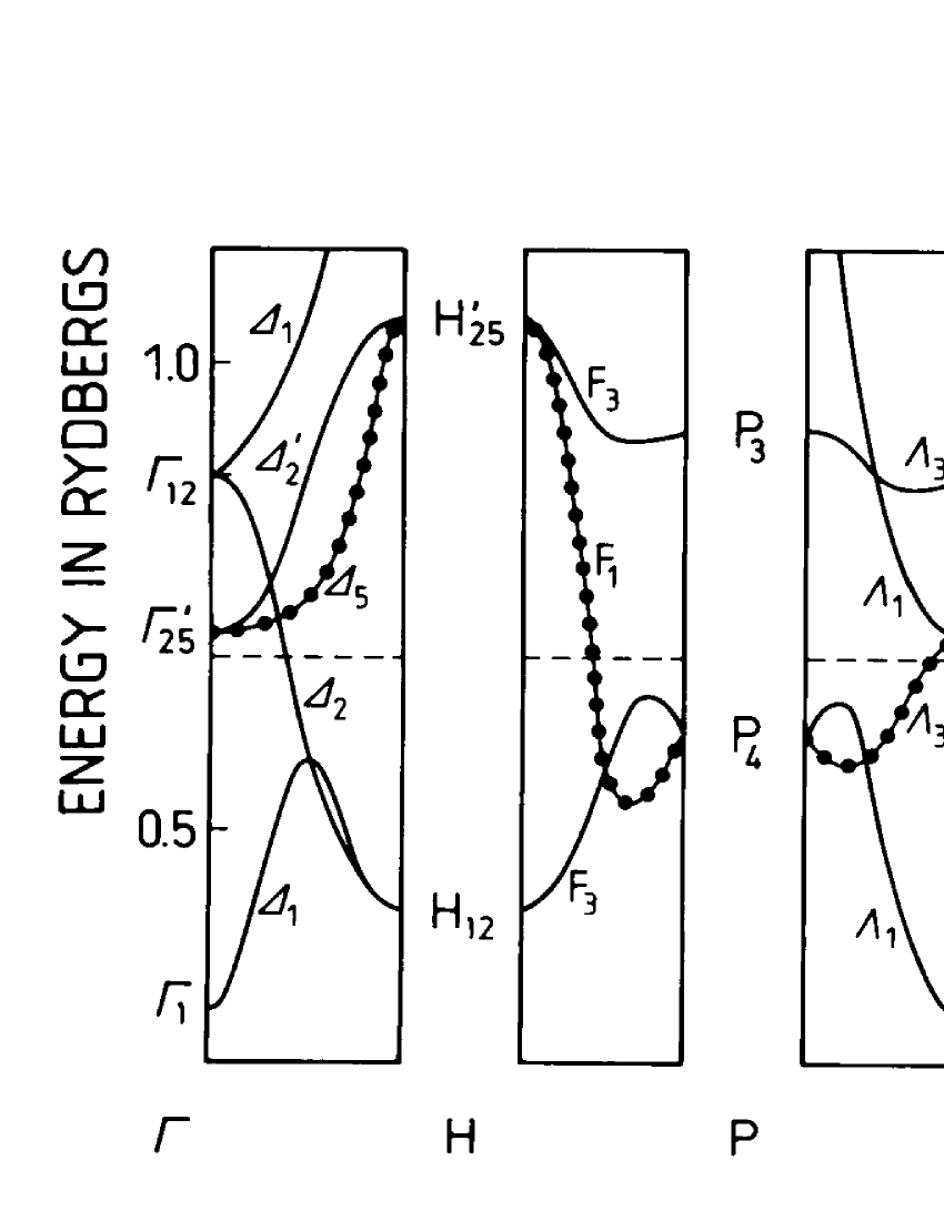
Figure 1: Band structure of Nb after Mattheis Mattheis (1969). The dotted line denotes the superconducting band.

Consider the superconducting band [Definition 7.6] of niobium in Fig. 1, as denoted by the dotted line. At the four points of symmetry $\Gamma$, $H$, $N$, and $P$ in the Brillouin zone for the space group $O^{9}_{h}$ of niobium, this band is characterized by the representations

$$\Gamma_{25}^{\prime},\ H_{25}^{\prime},\ N_{2},\text{ and }P_{4}$$

of $O^{9}_{h}$ in the familiar notation of Bouckaert, Smoluchowski and Wigner Bouckaert et al. (1936), which may be written as

$$\Gamma^{+}_{5},\ H^{+}_{5},\ N^{+}_{4},\text{ and }P_{5},$$ (7.79)

respectively, in the notation of Bradley and Cracknell  Bradley and A.P.Cracknell (1972) (see Tables 5.7 and 5.8 ibidem) which is consistently used in our papers. When we take into account that the electrons possess a spin, we receive

$$\begin{array}[]{lllllll}\Gamma^{+}_{5}&\otimes&d_{1/2}&=&\Gamma_{7}^{+}&\oplus&\Gamma_{8}^{+},\\ H^{+}_{5}&\otimes&d_{1/2}&=&H_{7}^{+}&\oplus&H_{8}^{+},\\ P_{5}&\otimes&d_{1/2}&=&P_{7}&\oplus&P_{8},\\ N^{+}_{4}&\otimes&d_{1/2}&=&N_{5}^{+}.\end{array}$$

Hence, at the points $\Gamma$, $H$, $P$, and $N$ the Bloch spinors can be transformed in such a way that at each of the four points $\Gamma$, $H$, $N$, and $P$ two spinors form basis functions for the double-valued representations

$$\Gamma_{7}^{+},\ H_{7}^{+},\ P_{7},\text{ and }N_{5}^{+},$$ (7.80)

respectively. We may unitarily transform the Bloch spinors $\psi_{\bm{k},q,s}(\bm{r},t)$ of this single energy band characterized by the representations (7.80) into best localized and symmetry-adapted spin-dependent Wannier functions because Theorem 7.2 yields with $H_{0}=O_{h}$, $\mu=1$, $\bm{\rho}_{1}=\bm{0}$, $G_{0p}=H_{0}=O_{h}$, and $\bm{d}_{1}=\Gamma^{+}_{2}$ first the single-valued representations

$$\bm{D}^{\text{aff}}_{\Gamma}=\Gamma^{+}_{2},\ \bm{D}^{\text{aff}}_{H}=H^{+}_{2},\ \bm{D}^{\text{aff}}_{P}=P_{2},\ \text{and}\ \bm{D}^{\text{aff}}_{N}=N^{+}_{3}$$ (7.81)

and then, with Eq. (7.28), the double-valued representations (7.80).

The representations in Eq. (7.81) define (the only) single-valued band affiliated to the superconducting band defined by the representations in Eq. (7.80) [Definition 7.4]. The representation $\bm{D}$ defining the spin-dependent Wannier functions [Definition 7.3] is equal to $\Gamma^{+}_{2}$,

$$\bm{D}=\Gamma^{+}_{2}.$$ (7.82)

$\bm{D}$ is one-dimensional since we have one Nb atom in the unit cell. The spin-dependent Wannier functions may be chosen symmetry-adapted to the magnetic group in Eq. (7.29) because $\Gamma^{+}_{2}$ is real.

The Bloch functions of the superconducting band cannot be unitarily transformed into usual Wannier functions which are best localized and symmetry-adapted to $O^{9}_{h}$ since it was not closed before the spin-dependent perturbation $\mathcal{H}_{s}$ was activated. Thus [Theorem 7.5], we cannot choose the matrix ${\bf f}(1,\bm{k})$ in Eq. (7.3) (with $q=1$ since we only have one branch in the superconducting band of Nb) independent of $\bm{k}$ when we demand that the Wannier functions are best localized and symmetry-adapted. This important statement shall be demonstrated by an example:

Consider the point $N$ with the wave vector $\bm{k}_{N}$ in the first domain of the Brillouin zone for $O^{9}_{h}$. The representations $\bm{d}_{\bm{k}_{N},1}^{\text{aff}}$ and $\bm{d}_{\bm{k}_{N},1}$ in Eq. (7.69) are given by Eqs. (7.81) and (7.79),

$$\bm{d}_{\bm{k}_{N},1}^{\text{aff}}=N^{+}_{3}$$ (7.83)

and

$$\bm{d}_{\bm{k}_{N},1}=N^{+}_{4}.$$ (7.84)

Thus, Eq. (7.69) may be written as

$$N^{+}_{4}\otimes\bm{d}_{1/2}=\\ ({\bf f}^{*}(1,\bm{k}_{N}))^{-1}\cdot(N^{+}_{3}\otimes\bm{d}_{1/2})\cdot{\bf f}^{*}(1,\bm{k}_{N}).$$ (7.85)

This equation is solvable since both representations $N^{+}_{4}\otimes\bm{d}_{1/2}$ and $N^{+}_{3}\otimes\bm{d}_{1/2}$ are equivalent, but it is evidently not solved by ${\bf f}(1,\bm{k}_{N})={\bf 1}$. In fact, we receive

$${\bf f}(1,\bm{k}_{N})=\left(\begin{array}[]{cc}0&1\\ -i&0\end{array}\right)$$ (7.86)

by means of Tables 5.7 and 6.1 of Ref. Bradley and A.P.Cracknell (1972). This is the value of ${\bf f}(1,\bm{k})$ also on the planes of symmetry intersecting at $N$ in the neighborhood of $N$. Further away from $N$, however, ${\bf f}(1,\bm{k})$ may change since it is $\bm{k}$ dependent.

In the same way, we find

$${\bf f}(1,\bm{k}_{F})=\frac{1}{\sqrt{3}}\left(\begin{array}[]{cc}-i&-1+i\\ 1+i&i\end{array}\right)$$ (7.87)

for the points $\bm{k}_{F}$ on the line $F$.

Eqs. (7.86) and (7.87) demonstrate that ${\bf f}(1,\bm{k})$ cannot be chosen independent of $\bm{k}$ in the superconducting band of niobium.

VIII Conclusion

In the present paper we gave the group theory of best localized and symmetry-adapted Wannier functions with the expectation that it will be helpful to determine the symmetry of the Wannier functions in the band structure of any given material. The paper is written in such a way that it should be possible to create a computer program automating the determination of Wannier functions.

In this paper we restricted ourselves to Wannier functions that define magnetic or superconducting bands. That means that we only considered Wannier functions centered at the atomic positions. When other physical phenomena shall be explored, as, e.g., the metallic bound, other Wannier functions may be needed which are centered at other positions, e.g., between the atoms. It should be noted that Refs. Krüger (1972a), Krüger (1972b) and Krüger (1974) define best localized and symmetry-adapted Wannier functions in general terms which may be centered at a variety of positions $\bm{\rho}_{i}$ being different from the positions of the atoms.