Weitzenböck’s Torsion, Fermi Coordinates and Adapted Frames

Abstract

We study Weitzenböck’s torsion and discuss its properties. Specifically, we calculate the measured components of Weitzenböck’s torsion tensor for a frame field adapted to static observers in a Fermi normal coordinate system that we establish along the world line of an arbitrary accelerated observer in general relativity. A similar calculation is carried out in the standard Schwarzschild-like coordinates for static observers in the exterior Kerr spacetime; we then compare our results with the corresponding curvature components. Our work supports the contention that in the extended general relativistic framework involving both the Levi-Civita and Weitzenböck connections, curvature and torsion provide complementary representations of the gravitational field.

I Introduction

It is possible to extend the pseudo-Riemannian (i.e., Lorentzian) structure of General Relativity (GR) in a natural way by adding a second nonsymmetric connection due to Weitzenböck We . The Weitzenböck connection is related to congruent frames adapted to observer families LB . The standard Levi-Civita connection (${}^{0}\Gamma^{\mu}_{\alpha\beta}$) is symmetric and hence torsion-free, but gives rise to the Riemannian curvature of spacetime that characterizes the gravitational field in GR. On the other hand, the Weitzenböck connection ($\Gamma^{\mu}_{\alpha\beta}$), which is compatible with the Riemannian metric ($g_{\mu\nu}$), is curvature-free, but has torsion. The curvature of the Levi-Civita connection and the torsion of the Weitzenböck connection are complementary aspects of the gravitational field in the recent nonlocal generalization of GR HM1 ; HM2 ; RM ; Mas .

In a global inertial frame in Minkowski spacetime, there exists a natural system of globally parallel tetrad frames, since the ideal inertial observers at rest carry orthonormal tetrad frames that consist of the four unit basis vectors of the background inertial frame in which the observers are all at rest. Flat spacetime contains an equivalence class of such parallel frame fields that are related to each other by constant elements of the six-parameter global Lorentz group. This parallelism disappears in the curved spacetime of GR. That is, given any smooth orthonormal tetrad field $\lambda^{\mu}{}_{\hat{\alpha}}(x)$ adapted to an observer family in curved spacetime, it is not possible to render the frame field parallel in any spacetime domain due to the presence of the Riemannian curvature of the Levi-Civita connection. It is nevertheless useful to have access to a global system of parallel axes in the presence of gravitation. To this end, one must extend GR by introducing a second (Weitzenböck) connection, which is so defined as to render a smooth orthonormal frame field parallel in extended GR. Therefore, of all possible smooth frame fields on Riemannian spacetime, one system can be chosen in order to define a global system of parallel axes that are, however, specified up to global Lorentz transformations. This circumstance is reminiscent of the parallel frame fields of inertial observers in Minkowski spacetime. In extended GR, the chosen parallel frame field is adapted to a preferred family of observers. Such an observer family is then unique up to global Lorentz transformations, just as is the case with inertial observers in Minkowski spacetime. Henceforth, a preferred observer family in extended GR is one for which the frame field is globally parallel via the Weitzenböck connection.

Imagine a class of preferred observers in extended GR and their associated smooth tetrad frame field $e^{\mu}{}_{\hat{\alpha}}$ such that

$$g_{\mu\nu}\,e^{\mu}{}_{\hat{\alpha}}\,e^{\nu}{}_{\hat{\beta}}=\eta_{\hat{\alpha}\hat{\beta}}\,,$$ (1)

which is the orthonormality condition for the frame field. For this class of preferred observers, the Weitzenböck connection is given by We

$$\Gamma^{\mu}_{\alpha\beta}=e^{\mu}{}_{\hat{\nu}}\,\partial_{\alpha}\,e_{\beta}{}^{\hat{\nu}}\,.$$ (2)

This is essentially the unique connection for which the corresponding covariant differentiation is such that $\nabla_{\nu}\,e_{\mu}{}^{\hat{\alpha}}=0$. From this and the orthonormality condition, we get metric compatibility; that is, $\nabla_{\nu}\,g_{\alpha\beta}=0$. This leads to a global notion of parallelism; namely, distant vectors may be considered parallel if they have the same local components relative to their preferred frames. Teleparallelism has a long history HS ; BH ; AP ; Mal ; in this framework, GR has an equivalent teleparallel formulation (GR_||) Mo ; PP .

The difference between two connections on the same manifold is a tensor. Thus we have the torsion tensor

$$C_{\alpha\beta}{}^{\mu}=\Gamma^{\mu}_{\alpha\beta}-\Gamma^{\mu}_{\beta\alpha}=e^{\mu}{}_{\hat{\nu}}\left(\partial_{\alpha}\,e_{\beta}{}^{\hat{\nu}}-\partial_{\beta}\,e_{\alpha}{}^{\hat{\nu}}\right)\,,$$ (3)

and the contorsion tensor

$$K_{\alpha\beta}{}^{\mu}={}^{0}\Gamma^{\mu}_{\alpha\beta}-\Gamma^{\mu}_{\alpha\beta}\,.$$ (4)

It follows from the compatibility of the Levi-Civita and Weitzenböck connections with the Riemannian metric that the contorsion tensor is linearly related to the torsion tensor via

$$K_{\alpha\beta\gamma}=\frac{1}{2}(C_{\alpha\gamma\beta}+C_{\beta\gamma\alpha}-C_{\alpha\beta\gamma})\,.$$ (5)

We note that the torsion tensor is antisymmetric in its first two indices, while the contorsion tensor is antisymmetric in its last two indices. In this paper, we choose units such that $G=c=1$. Furthermore, Greek indices run from 0 to 3, while Latin indices run from 1 to 3. The signature of the metric is +2. We use a left superscript “0” for geometric quantities related to the Levi-Civita connection. Our conventions regarding the use of a nonsymmetric connection are explained in Appendix A.

Let us consider the frame components of the Weitzenböck torsion with respect to the preferred orthonormal frame $e_{\hat{\alpha}}$ with dual $\omega^{\hat{\alpha}}$ such that $\omega^{\hat{\alpha}}(e_{\hat{\beta}})=\delta^{\hat{\alpha}}_{\hat{\beta}}$; that is,

$$C_{\hat{\alpha}\hat{\beta}}{}^{\hat{\gamma}}=e^{\mu}{}_{\hat{\alpha}}\,e^{\nu}{}_{\hat{\beta}}\left(\partial_{\mu}\,e_{\nu}{}^{\hat{\gamma}}-\partial_{\nu}\,e_{\mu}{}^{\hat{\gamma}}\right)\,.$$ (6)

These are measurable in principle and are essentially the structure functions of the preferred frame $e_{\hat{\alpha}}=e^{\mu}{}_{\hat{\alpha}}\,\partial_{\mu}$; that is,

$$[e_{\hat{\alpha}}\,,e_{\hat{\beta}}]=-C_{\hat{\alpha}\hat{\beta}}{}^{\hat{\gamma}}\,e_{\hat{\gamma}}\,.$$ (7)

Equivalently, these components can be obtained by evaluating the exterior derivative of the frame $1$-forms $\omega^{\hat{\gamma}}=e_{\mu}{}^{\hat{\gamma}}\,dx^{\mu}$ according to the relation

$$d\omega^{\hat{\gamma}}=\frac{1}{2}C_{\hat{\alpha}\hat{\beta}}{}^{\hat{\gamma}}\,\omega^{\hat{\alpha}}\wedge\omega^{\hat{\beta}}\,,$$ (8)

or the Lie derivative of the frame vectors along each other

$$\pounds_{e_{\hat{\alpha}}}\,e_{\hat{\beta}}=[e_{\hat{\alpha}}\,,e_{\hat{\beta}}]=-C_{\hat{\alpha}\hat{\beta}}{}^{\hat{\gamma}}\,e_{\hat{\gamma}}\,$$ (9)

and its “dual” relation

$$\pounds_{e_{\hat{\alpha}}}\,\omega^{\hat{\beta}}=C_{\hat{\alpha}\hat{\gamma}}{}^{\hat{\beta}}\omega^{\hat{\gamma}}\,.$$ (10)

At any event in spacetime, two orthonormal frames are related to each other by an element of the local Lorentz group; therefore, $C_{\hat{\alpha}\hat{\beta}}{}^{\hat{\gamma}}$ transforms as a third-rank tensor under local Lorentz transformations. Moreover, these structure functions satisfy the Jacobi identity,

$$[e_{\hat{\alpha}}\,,[e_{\hat{\beta}}\,,e_{\hat{\gamma}}]\,]+[e_{\hat{\beta}}\,,[e_{\hat{\gamma}}\,,e_{\hat{\alpha}}]\,]+[e_{\hat{\gamma}}\,,[e_{\hat{\alpha}}\,,e_{\hat{\beta}}]\,]=0\,,$$ (11)

which is equivalent to $d^{2}\omega^{\hat{\alpha}}=0$. It follows from the Jacobi identity that

$$\partial_{\,[\,\hat{\alpha}}\,C_{\hat{\beta}\hat{\gamma}]\,}{}^{\hat{\mu}}+C_{\hat{\sigma}[\hat{\alpha}}{}^{\hat{\mu}}\,C_{\hat{\beta}\hat{\gamma}]}{}^{\hat{\sigma}}=0\,,$$ (12)

where $\partial_{\hat{\alpha}}:=e_{\hat{\alpha}}$ is the Pfaffian derivative associated with $e_{\hat{\alpha}}$.

The main purpose of this paper is to calculate the structure functions $C_{\hat{\alpha}\hat{\beta}}{}^{\hat{\gamma}}$ in a general and physically transparent setting and study their physical properties. The following section is devoted to the study of the structure functions in the physically meaningful Fermi coordinates in a general gravitational field. In section III, we examine the structure functions for static observers in a general stationary axisymmetric gravitational field such as the Kerr spacetime. Section IV is devoted to a brief discussion of the lack of closure of infinitesimal parallelograms in the presence of torsion. Finally, section V contains a discussion of our results.

II Weitzenböck’s Torsion in Fermi Coordinates

To gain physical insight into the structure of Weitzenböck’s torsion, we consider an arbitrary gravitational field in extended GR and establish a Fermi coordinate system in a cylindrical spacetime region along the world line of an arbitrary accelerated observer ${\cal O}$. Fermi coordinates are invariantly defined and constitute the natural general-relativistic generalization of inertial Cartesian coordinates. We then define the frame field of static observers in the Fermi coordinate system and calculate explicitly their measured torsion tensor $C_{\hat{\alpha}\hat{\beta}}{}^{\hat{\gamma}}$.

Imagine an accelerated observer ${\cal O}$ following the reference world line ${\bar{x}}^{\mu}(\tau)$, where $x^{\mu}=(t,x^{i})$ is an admissible system of spacetime coordinates BCM and $\tau$ is the proper time along the observer’s trajectory. The observer carries an orthonormal tetrad frame $\lambda^{\mu}{}_{\hat{\alpha}}(\tau)$ along its path in accordance with

$$\frac{{}^{0}D\lambda^{\mu}{}_{\hat{\alpha}}}{d\tau}=\phi_{\hat{\alpha}}{}^{\hat{\beta}}(\tau)~{}\lambda^{\mu}{}_{\hat{\beta}}\,.$$ (13)

Here, $\phi_{\hat{\alpha}\hat{\beta}}=-\phi_{\hat{\beta}\hat{\alpha}}$ is the acceleration tensor of ${\cal O}$. In close analogy with the Faraday tensor, we can decompose the acceleration tensor into its “electric” and “magnetic” components, namely, $\phi_{\hat{\alpha}\hat{\beta}}\mapsto(-\mathbf{a},\bm{\Omega})$. That is, the translational acceleration vector $\mathbf{a}$ is given by the frame components of the 4-acceleration vector associated with the 4-velocity vector $\lambda^{\mu}{}_{\hat{0}}=d{\bar{x}}^{\mu}/d\tau$ of the observer and $\bm{\Omega}$ is the angular velocity of the rotation of the observer’s local spatial triad $\lambda^{\mu}{}_{\hat{i}}$ ,  $i=1,2,3$, with respect to the locally nonrotating (i.e., Fermi-Walker transported) triad Mash .

Let us next establish an extended Fermi normal coordinate system in a world tube along ${\bar{x}}^{\mu}(\tau)$. The Fermi coordinates are scalar invariants by construction and are indispensable for the interpretation of measurements in GR—see Sy ; BMash ; NZ ; CM1 ; CM2 ; CM3 and the references cited therein. Consider the class of spacelike geodesics that are orthogonal to the world line of the accelerated observer at each event $Q(\tau)$ along ${\bar{x}}^{\mu}(\tau)$. These form a local hypersurface. For an event $P$ with coordinates $x^{\mu}$ on this hypersurface, let there be a unique spacelike geodesic of proper length $\sigma$ that connects $Q$ to $P$. Then, $P$ has Fermi coordinates $X^{\hat{\mu}}=(T,X^{\hat{i}})$, where

$$T=\tau\,,\qquad X^{\hat{i}}=\sigma\,\xi^{\mu}\,\lambda_{\mu}{}^{\hat{i}}(\tau)\,.$$ (14)

Here, $\xi^{\mu}$ is the unit vector at $Q(\tau)$ that is tangent to the spacelike geodesic segment from $Q$ to $P$. Thus the reference observer $\cal{O}$ is always at the spatial origin of the Fermi coordinate system.

The coordinate transformation $x^{\mu}\mapsto(X^{\hat{0}}=T,X^{\hat{a}})$ can only be specified implicitly in general; hence, it is useful to express the spacetime metric in Fermi coordinates as a Taylor expansion in powers of the spatial distance $\sigma$ away from the reference world line. For our present purposes, we can write the metric in Fermi coordinates as

$$g_{\hat{0}\hat{0}} = -{\cal P}^{2}+{\cal Q}^{2}-R_{\hat{0}\hat{i}\hat{0}\hat{j}}X^{\hat{i}}X^{\hat{j}}+O(|\mathbf{X}|^{3})\,,$$

$$= -{\cal P}^{2}+{\cal Q}^{2}-2\Phi+O(|\mathbf{X}|^{3})\,,$$

$$g_{\hat{0}\hat{i}} = {\cal Q}_{\hat{i}}-\frac{2}{3}R_{\hat{0}\hat{j}\hat{i}\hat{k}}X^{\hat{j}}X^{\hat{k}}+O(|\mathbf{X}|^{3})\,,$$

$$= {\cal Q}_{\hat{i}}-2{\mathcal{A}}_{\hat{i}}+O(|\mathbf{X}|^{3})\,,$$

$$g_{\hat{i}\hat{j}} = \delta_{\hat{i}\hat{j}}-\frac{1}{3}R_{\hat{i}\hat{k}\hat{j}\hat{l}}X^{\hat{k}}X^{\hat{l}}+O(|\mathbf{X}|^{3})\,,$$ (15)

$$= \delta_{\hat{i}\hat{j}}-2\Sigma_{\hat{i}\hat{j}}+O(|\mathbf{X}|^{3})\,.$$

Here, we have introduced

$${\cal P}=1+U\,,\qquad U={\mathbf{a}}\cdot{\mathbf{X}}\,,\qquad\mathbf{{\cal Q}}=\bm{\Omega}\times{\mathbf{X}}\,$$ (16)

and we have used the notation

$$\Phi=\frac{1}{2}R_{\hat{0}\hat{i}\hat{0}\hat{j}}X^{\hat{i}}X^{\hat{j}}\,,\qquad{\mathcal{A}}_{\hat{i}}=\frac{1}{3}R_{\hat{0}\hat{j}\hat{i}\hat{k}}X^{\hat{j}}X^{\hat{k}}\,,\qquad\Sigma_{\hat{i}\hat{j}}=\frac{1}{6}R_{\hat{i}\hat{k}\hat{j}\hat{l}}X^{\hat{k}}X^{\hat{l}}\,.$$ (17)

Moreover, $R_{\hat{\alpha}\hat{\beta}\hat{\gamma}\hat{\delta}}(T)$ is the projection of the Riemann curvature tensor on the orthonormal tetrad frame of ${\cal O}$ and evaluated along the reference geodesic; that is,

$$R_{\hat{\alpha}\hat{\beta}\hat{\gamma}\hat{\delta}}(T):=\,^{0}R_{\mu\nu\rho\sigma}\,\lambda^{\mu}{}_{\hat{\alpha}}\,\lambda^{\nu}{}_{\hat{\beta}}\,\lambda^{\rho}{}_{\hat{\gamma}}\,\lambda^{\sigma}{}_{\hat{\delta}}\,.$$ (18)

Henceforward, we will only keep terms up to second-order in the metric perturbation and note that Fermi coordinates are admissible in a finite cylindrical region about the world line of ${\cal O}$ with $|\mathbf{X}|\ll r_{c}$, where $r_{c}(T)$ is the infimum of acceleration lengths $(|\mathbf{a}(T)|^{-1},|\bm{\Omega}(T)|^{-1})$ as well as spacetime curvature lengths such as $|R_{\hat{\alpha}\hat{\beta}\hat{\gamma}\hat{\delta}}(T)|^{-1/2}$.

Let us now consider the class of observers that are all at rest in this gravitational field and carry orthonormal tetrads that have essentially the same orientation as the Fermi coordinate system. This class includes of course our reference observer ${\cal O}$. The orthonormal tetrad frame of these preferred observers can be expressed in $(T,X^{\hat{i}})$ coordinates as

$$e^{\mu}{}_{\hat{0}} =(1-\tilde{\Phi},\,0,\,0,\,0)\,,$$ (19)

$$e^{\mu}{}_{\hat{1}} =(-2\tilde{{\cal A}}_{\hat{1}},\,1+\tilde{\Sigma}_{\hat{1}\hat{1}},\,0,\,0)\,,$$ (20)

$$e^{\mu}{}_{\hat{2}} =(-2\tilde{{\cal A}}_{\hat{2}},\,2\,\tilde{\Sigma}_{\hat{2}\hat{1}},\,1+\tilde{\Sigma}_{\hat{2}\hat{2}},\,0)\,,$$ (21)

$$e^{\mu}{}_{\hat{3}} =(-2\tilde{{\cal A}}_{\hat{3}},\,2\,\tilde{\Sigma}_{\hat{3}\hat{1}},\,2\,\tilde{\Sigma}_{\hat{3}\hat{2}},\,1+\tilde{\Sigma}_{\hat{3}\hat{3}})\,.$$ (22)

Here, we have defined

$$\tilde{\Phi}:=\Phi+U-U^{2}-\frac{1}{2}{\cal Q}^{2}\,,\quad\tilde{{\cal A}}_{\hat{i}}:={\cal A}_{\hat{i}}-(\frac{1}{2}-U){\cal Q}_{\hat{i}}\,,\quad\tilde{\Sigma}_{\hat{i}\hat{j}}:=\Sigma_{\hat{i}\hat{j}}-\frac{1}{2}{\cal Q}_{\hat{i}}{\cal Q}_{\hat{j}}\,.$$ (23)

As expected, $e^{\mu}{}_{\hat{\alpha}}$ reduces to $\delta^{\mu}_{\hat{\alpha}}$ along the reference geodesic, where $\mathbf{X}=0$. It follows from $e_{\mu\hat{\alpha}}=g_{\mu\nu}\,e^{\nu}{}_{\hat{\alpha}}$ that

$$e_{\mu\,\hat{0}} =(-1-U^{2}-\tilde{\Phi},\,-2\tilde{{\cal A}}_{\hat{1}}+U{\cal Q}_{\hat{1}},\,-2\tilde{{\cal A}}_{\hat{2}}+U{\cal Q}_{\hat{2}},\,-2\tilde{{\cal A}}_{\hat{3}}+U{\cal Q}_{\hat{3}})\,,$$ (24)

$$e_{\mu\,\hat{1}} =(0,\,1-\tilde{\Sigma}_{\hat{1}\hat{1}},\,-2\,\tilde{\Sigma}_{\hat{1}\hat{2}},\,-2\,\tilde{\Sigma}_{\hat{1}\hat{3}})\,,$$ (25)

$$e_{\mu\,\hat{2}} =(0,\,0,\,1-\tilde{\Sigma}_{\hat{2}\hat{2}},\,-2\,\tilde{\Sigma}_{\hat{2}\hat{3}})\,,$$ (26)

$$e_{\mu\,\hat{3}} =(0,\,0,\,0,\,1-\tilde{\Sigma}_{\hat{3}\hat{3}})\,.$$ (27)

Explicitly, we therefore have

$$e_{\hat{0}} = \left(1-U+U^{2}+\frac{1}{2}{\cal Q}^{2}-\Phi\right)\partial_{T}\,,$$

$$e_{\hat{1}} = \left[-2{\mathcal{A}}_{\hat{1}}+{\cal Q}_{\hat{1}}(1-2U)\right]\partial_{T}+\left(1-\frac{1}{2}{\cal Q}_{\hat{1}}^{2}+\Sigma_{\hat{1}\hat{1}}\right)\partial_{X^{\hat{1}}}\,,$$

$$e_{\hat{2}} = \left[-2{\mathcal{A}}_{\hat{2}}+{\cal Q}_{\hat{2}}(1-2U)\right]\partial_{T}+\left(2\Sigma_{\hat{2}\hat{1}}-{\cal Q}_{\hat{2}}{\cal Q}_{\hat{1}}\right)\partial_{X^{\hat{1}}}+\left(1-\frac{1}{2}{\cal Q}_{\hat{2}}^{2}+\Sigma_{\hat{2}\hat{2}}\right)\partial_{X^{\hat{2}}}\,,$$

$$e_{\hat{3}} = \left[-2{\mathcal{A}}_{\hat{3}}+{\cal Q}_{\hat{3}}(1-2U)\right]\partial_{T}+\left(2\Sigma_{\hat{3}\hat{1}}-{\cal Q}_{\hat{3}}{\cal Q}_{\hat{1}}\right)\partial_{X^{\hat{1}}}+\left(2\Sigma_{\hat{3}\hat{2}}-{\cal Q}_{\hat{3}}{\cal Q}_{\hat{2}}\right)\partial_{X^{\hat{2}}}$$ (28)

$$+\left(1-\frac{1}{2}{\cal Q}_{\hat{3}}^{2}+\Sigma_{\hat{3}\hat{3}}\right)\partial_{X^{\hat{3}}}$$

with dual frame

$$\omega^{\hat{0}} = \left(1+U-\frac{1}{2}Q^{2}+\Phi\right)dT+[2{\mathcal{A}}_{\hat{a}}-{\cal Q}_{\hat{a}}(1-U)]dX^{\hat{a}}\,,$$

$$\omega^{\hat{1}} = \left(1+\frac{1}{2}{\cal Q}_{\hat{1}}^{2}-\Sigma_{\hat{1}\hat{1}}\right)dX^{\hat{1}}+\left({\cal Q}_{\hat{1}}{\cal Q}_{\hat{2}}-2\Sigma_{\hat{1}\hat{2}}\right)dX^{\hat{2}}+\left({\cal Q}_{\hat{1}}{\cal Q}_{\hat{3}}-2\Sigma_{\hat{1}\hat{3}}\right)dX^{\hat{3}}\,,$$

$$\omega^{\hat{2}} = \left(1+\frac{1}{2}{\cal Q}_{\hat{2}}^{2}-\Sigma_{\hat{2}\hat{2}}\right)dX^{\hat{2}}+\left({\cal Q}_{\hat{2}}{\cal Q}_{\hat{3}}-2\Sigma_{\hat{2}\hat{3}}\right)dX^{\hat{3}}\,,$$

$$\omega^{\hat{3}} = \left(1+\frac{1}{2}{\cal Q}_{\hat{3}}^{2}-\Sigma_{\hat{3}\hat{3}}\right)dX^{\hat{3}}\,.$$ (29)

We can now proceed to the evaluation of the associated structure functions.

In $C_{\hat{\alpha}\hat{\beta}}{}^{\hat{\gamma}}$, for each $\hat{\gamma}=\hat{0},\hat{1},\hat{2},\hat{3}$, we have an antisymmetric tensor that has “electric” and “magnetic” components in analogy with the Faraday tensor. Indeed, for $\hat{\gamma}=\hat{0}$, we have

$$C_{\hat{0}\hat{i}}{}^{\hat{0}}=-\left[\bm{{\cal E}}+(1-U)\mathbf{a}+\bm{\Omega}\times{\bm{{\cal Q}}}+\dot{\bm{{\cal Q}}}\right]_{\hat{i}}\,,\quad C_{\hat{i}\hat{j}}{}^{\hat{0}}=2\epsilon_{\hat{i}\hat{j}\hat{k}}\left[\bm{{\cal B}}-(1-U)\,\bm{\Omega}+{\mathbf{a}}\times\bm{{\cal Q}}\right]^{\hat{k}}\,,$$ (30)

where

$$\dot{\bm{{\cal Q}}}=\left(\frac{d\bm{\Omega}}{dT}\right)\times\mathbf{X}\,,\qquad{\mathbf{a}}\times\bm{{\cal Q}}=U\bm{\Omega}-(\mathbf{a}\cdot\bm{\Omega})\mathbf{X}\,.$$ (31)

Furthermore, the gravitoelectric field, $\bm{{\cal E}}=\bm{\nabla}\Phi$, and the gravitomagnetic field, $\bm{{\cal B}}=\bm{\nabla}\times\bm{{\cal A}}$ , are given by

$${\cal E}_{\hat{i}}(T,{\bf X})=R_{\hat{0}\hat{i}\hat{0}\hat{j}}(T)X^{\hat{j}}\,,\qquad{\cal B}_{\hat{i}}(T,{\bf X})=-\frac{1}{2}\epsilon_{\hat{i}\hat{j}\hat{k}}R^{\hat{j}\hat{k}}{}_{\hat{0}\hat{l}}(T)X^{\hat{l}}\,.$$ (32)

Let us note here that the gravitoelectric field is directly proportional to the “electric” components of the Riemann curvature tensor and similarly the gravitomagnetic field is directly proportional to the “magnetic” components of the Riemann curvature tensor. It is interesting that we can couch our torsion results in the familiar language of gravitoelectromagnetism (GEM) Matt ; JCB ; Mashhoon . Moreover, the spatial part of the metric perturbation away from Minkowski spacetime, $\Sigma_{ij}=\Sigma_{ji}$, is likewise proportional to the spatial components of the curvature. Next, for $\hat{\gamma}=\hat{1},\hat{2},\hat{3}$, the electric parts only involve terms of higher order and can be ignored, so that

$$C_{\hat{0}\hat{i}}{}^{\hat{j}}=0\,.$$ (33)

However, the corresponding magnetic parts depend upon the spatial components of the curvature and we find that for $\hat{\gamma}=\hat{1}$,

$$C_{\hat{2}\hat{3}}{}^{\hat{1}}=3\Omega_{\hat{1}}{\cal Q}_{\hat{1}}+R_{\hat{2}\hat{3}\hat{1}\hat{a}}X^{\hat{a}}\,,\quad C_{\hat{3}\hat{1}}{}^{\hat{1}}=2\Omega_{\hat{2}}{\cal Q}_{\hat{1}}+\frac{2}{3}R_{\hat{3}\hat{1}\hat{1}\hat{a}}X^{\hat{a}}\,,\quad C_{\hat{1}\hat{2}}{}^{\hat{1}}=2\Omega_{\hat{3}}{\cal Q}_{\hat{1}}+\frac{2}{3}R_{\hat{1}\hat{2}\hat{1}\hat{a}}X^{\hat{a}}\,.$$ (34)

Similarly, for $\hat{\gamma}=\hat{2}$,

$$C_{\hat{2}\hat{3}}{}^{\hat{2}} = 2\Omega_{\hat{1}}{\cal Q}_{\hat{2}}+\frac{2}{3}R_{\hat{2}\hat{3}\hat{2}\hat{a}}X^{\hat{a}}\,,\quad C_{\hat{3}\hat{1}}{}^{\hat{2}}=\Omega_{\hat{2}}{\cal Q}_{\hat{2}}-\Omega_{\hat{3}}{\cal Q}_{\hat{3}}+\frac{1}{3}(R_{\hat{3}\hat{1}\hat{2}\hat{a}}-R_{\hat{1}\hat{2}\hat{3}\hat{a}})X^{\hat{a}}\,,$$

$$\quad C_{\hat{1}\hat{2}}{}^{\hat{2}} = \Omega_{\hat{3}}{\cal Q}_{\hat{2}}+\frac{1}{3}R_{\hat{1}\hat{2}\hat{2}\hat{a}}X^{\hat{a}}\,,$$ (35)

and for $\hat{\gamma}=\hat{3}$,

$$C_{\hat{2}\hat{3}}{}^{\hat{3}}=\Omega_{\hat{1}}{\cal Q}_{\hat{3}}+\frac{1}{3}R_{\hat{2}\hat{3}\hat{3}\hat{a}}X^{\hat{a}}\,,\quad C_{\hat{3}\hat{1}}{}^{\hat{3}}=\Omega_{\hat{2}}{\cal Q}_{\hat{3}}+\frac{1}{3}R_{\hat{3}\hat{1}\hat{3}\hat{a}}X^{\hat{a}}\,,\quad C_{\hat{1}\hat{2}}{}^{\hat{3}}=0\,.$$ (36)

It is important to note that all of the components of $C_{\hat{\alpha}\hat{\beta}}{}^{\hat{\gamma}}$ can be obtained from Eqs. (30)–(36) by using the antisymmetry of $C_{\hat{\alpha}\hat{\beta}}{}^{\hat{\gamma}}$ in its first two indices. Furthermore, all of the components of the curvature tensor are involved in our calculation of the torsion tensor. The spatial components of the curvature tensor in Eqs. (34)–(36) essentially reduce to the gravitoelectric components in a Ricci-flat region of spacetime. The work reported here generalizes and extends the results of a previous investigation regarding the possibility of measurement of Weitzenböck’s torsion BaMa .

The torsion vector $C_{\alpha}$, $C_{\alpha}:=-C_{\alpha\beta}{}^{\beta}$, can be calculated for the static Fermi observers and turns out to be completely spatial; that is, $C_{\hat{\alpha}}=(0,\Theta_{\hat{i}})$, where $\bm{\Theta}$ is related to the gravitoelectric field as well as the spatial part of the torsion tensor. Indeed,

$$\Theta_{\hat{i}}=-\left[\bm{{\cal E}}+(1-U)\mathbf{a}+\bm{\Omega}\times{\bm{{\cal Q}}}+\dot{\bm{{\cal Q}}}\right]_{\hat{i}}-C_{\hat{i}\hat{j}}{}^{\hat{j}}\,.$$ (37)

On the other hand, the torsion pseudovector $\check{C}_{\alpha}$, $\check{C}_{\alpha}:=-(1/6)\epsilon_{\hat{\alpha}\hat{\beta}\hat{\gamma}\hat{\delta}}\,C^{\hat{\beta}\hat{\gamma}\hat{\delta}}$ is given by $(\check{C}_{\hat{0}},H_{\hat{i}})$, where $\check{C}_{\hat{0}}=-(1/3)(C_{\hat{2}\hat{3}}{}^{\hat{1}}+C_{\hat{3}\hat{1}}{}^{\hat{2}})$ and $\mathbf{H}$ is related to the gravitomagnetic field,

$$\mathbf{H}=\frac{2}{3}\,\left[\bm{{\cal B}}-(1-U)\,\bm{\Omega}+{\mathbf{a}}\times\bm{{\cal Q}}\right]\,.$$ (38)

We note that in our convention $\epsilon_{0123}=1$. The three algebraic Weitzenböck invariants of the torsion tensor are discussed in Appendix C.

It is interesting to compute the acceleration tensor for our family of static observers. To this end, we have

$$\frac{{}^{0}D\,e^{\mu}{}_{\hat{\alpha}}}{ds}=\Upsilon_{\hat{\alpha}}{}^{\hat{\beta}}~{}e^{\mu}{}_{\hat{\beta}}\,,$$ (39)

where $s$ is the proper time along the observer’s world line. From Eq. (4) and the fact that $e^{\mu}{}_{\hat{0}}=dx^{\mu}/ds$, we find that

$$\Upsilon_{\hat{\alpha}\hat{\beta}}=K_{\hat{0}\hat{\alpha}\hat{\beta}}\,.$$ (40)

Let us briefly digress here and mention that the connection between Eqs. (39) and (40) is completely general and is independent of the particular coordinate system or our choice of the preferred observers. In the particular case of Fermi coordinates and static observers under consideration here, however, it follows from the decomposition of $\Upsilon_{\hat{\alpha}\hat{\beta}}$ into its “electric” and “magnetic” components and Eq. (5) that $-C_{\hat{0}\hat{i}}{}^{\hat{0}}$ and $-\frac{1}{2}\,C_{\hat{i}\hat{j}}{}^{\hat{0}}$ are responsible for the proper acceleration and rotation of our observer family, respectively. This circumstance accounts for the nature of the terms that appear in Eq. (30), such as, for instance, the centripetal and transverse (Euler) acceleration terms in the electric components.

The torsion tensor vanishes along the reference world line $(\mathbf{X}=0)$ if $\phi_{\hat{\alpha}\hat{\beta}}=0$. It follows that along the reference geodesic, the contorsion tensor and the Weitzenböck connection both vanish. Thus, by a proper choice of coordinates and preferred frame field, the Levi-Civita connection as well as the Weitzenböck connection can be made to vanish along a timelike geodesic. This provides a natural generalization of Fermi’s result in the context of extended GR.

III Kerr Spacetime

Imagine accelerated observers at rest far away from a rotating gravitational source. Within the framework of linearized GR, the spacetime metric in gravitoelectromagnetic (GEM) form is given by Mashhoon

$$ds^{2}=-(1+2\Phi^{\prime})dt^{2}-4(\mathbf{A}\cdot d\mathbf{x})dt+(1-2\Phi^{\prime})\delta_{ij}dx^{i}dx^{j}\,,$$ (41)

where $\Phi^{\prime}$ is the gravitoelectric potential of the source and $\mathbf{A}$ is the corresponding gravitomagnetic vector potential. Following the linear perturbation approach, the GEM fields are given by Mashhoon

$$\mathbf{E}=\bm{\nabla}\Phi^{\prime}-\frac{\partial}{\partial t}\left(\frac{1}{2}\mathbf{A}\right)\,,\qquad\mathbf{B}=\bm{\nabla}\times\mathbf{A}\,.$$ (42)

The natural orthonormal tetrad frame adapted to these static observers can be expressed as

$$e^{\mu}{}_{\hat{0}} =(1-\Phi^{\prime},\,0,\,0,\,0)\,,$$ (43)

$$e^{\mu}{}_{\hat{1}} =(-2A_{\hat{1}},\,1+\Phi^{\prime},\,0,\,0)\,,$$ (44)

$$e^{\mu}{}_{\hat{2}} =(-2A_{\hat{2}},\,0,\,1+\Phi^{\prime},\,0)\,,$$ (45)

$$e^{\mu}{}_{\hat{3}} =(-2A_{\hat{3}},\,0,\,0,\,1+\Phi^{\prime})\,.$$ (46)

Taking into account the antisymmetry of the torsion tensor in its first two indices, all of the nonzero components of the structure functions can be obtained in this case from

$$C_{\hat{0}\hat{i}}{}^{\hat{0}}=-E_{\hat{i}}+\frac{3}{2}\,\partial_{t}\,A_{\hat{i}}\,,\qquad C_{\hat{i}\hat{j}}{}^{\hat{0}}=2\epsilon_{\hat{i}\hat{j}\hat{k}}\,B^{\hat{k}}\,$$ (47)

and

$$C_{\hat{i}\hat{\alpha}}{}^{\hat{j}}=\partial_{\alpha}\,\Phi^{\prime}\,\delta_{\hat{i}}^{\hat{j}}\,.$$ (48)

To illustrate further the nature of Weitzenböck’s torsion, we calculate in this section the structure functions for the natural tetrad frames of the static observers in the exterior Kerr spacetime. To this end, let us first consider the case of a general stationary metric of the form

$$ds^{2}=g_{00}(dx^{0}){}^{2}+g_{11}(dx^{1}){}^{2}+g_{22}(dx^{2}){}^{2}+2g_{03}dx^{0}dx^{3}+g_{33}(dx^{3}){}^{2}$$ (49)

where the metric coefficients $g_{\alpha\beta}$ depend only upon $x^{1}$ and $x^{2}$. A static observer in this case has a 4-velocity vector given by

$$e_{\hat{0}}=\frac{1}{\sqrt{-g_{00}}}\partial_{0}\,,$$ (50)

and a natural adapted spatial frame that consists of the three vectors

$$e_{\hat{1}}=\frac{1}{\sqrt{g_{11}}}\partial_{1}\,,\quad e_{\hat{2}}=\frac{1}{\sqrt{g_{22}}}\partial_{2}\,,\quad e_{\hat{3}}={\cal F}\,\left(-{\cal G}\,\partial_{0}+\partial_{3}\right)\,,$$ (51)

where

$${\cal F}:=\frac{1}{\sqrt{g_{33}-\frac{g_{03}^{2}}{g_{00}}}}\,,\qquad{\cal G}:=\frac{g_{03}}{g_{00}}\,.$$ (52)

Furthermore, we note that

$$\sqrt{-g}\,{\cal F}=\sqrt{-g_{00}\,g_{11}\,g_{22}}\,.$$ (53)

For the structure functions in this case, we have the following general results for the gravitoelectric components

$$C_{\hat{0}\hat{1}}{}^{\hat{0}}=\frac{1}{\sqrt{g_{11}}}\partial_{1}\ln\sqrt{-g_{00}}\,,\quad C_{\hat{0}\hat{2}}{}^{\hat{0}}=\frac{1}{\sqrt{g_{22}}}\partial_{2}\ln\sqrt{-g_{00}}\,,\quad C_{\hat{0}\hat{3}}{}^{\hat{0}}=0\,$$ (54)

and the corresponding gravitomagnetic components

$$C_{\hat{i}\hat{j}}{}^{\hat{0}}=\sqrt{-g_{00}}\,{\cal F}\,\epsilon_{\hat{i}\hat{j}\hat{k}}\,{\tilde{\cal G}}^{\hat{k}}\,,\qquad{\tilde{\cal G}}^{\hat{i}}:=\epsilon^{\hat{i}\hat{j}\hat{k}}\,\partial_{\hat{j}}\,(0,0,{\cal G})_{\hat{k}}=(\frac{1}{\sqrt{g_{22}}}\,\partial_{2}{\cal G},-\frac{1}{\sqrt{g_{11}}}\,\partial_{1}{\cal G},0)\,,$$ (55)

where $\partial_{\hat{i}}=e^{\mu}{}_{\hat{i}}\,\partial_{\mu}$ is the Pfaffian derivative operator. Moreover, $C_{\hat{0}\hat{i}}{}^{\hat{j}}=0$ and all of the other nonzero spatial components can be obtained from

$$C_{\hat{1}\hat{2}}{}^{\hat{1}}=-\frac{1}{\sqrt{g_{22}}}\,\partial_{2}\ln\sqrt{g_{11}}\,,\qquad C_{\hat{2}\hat{1}}{}^{\hat{2}}=-\frac{1}{\sqrt{g_{11}}}\,\partial_{1}\ln\sqrt{g_{22}}\,$$ (56)

and

$$C_{\hat{3}\hat{1}}{}^{\hat{3}}=\frac{1}{\sqrt{g_{11}}}\,\partial_{1}\ln{\cal F}\,,\qquad C_{\hat{3}\hat{2}}{}^{\hat{3}}=\frac{1}{\sqrt{g_{22}}}\,\partial_{2}\ln{\cal F}\,.$$ (57)

The torsion vector $C_{\alpha}$ can be easily calculated from these results and we find that $C_{\hat{\alpha}}=(0,C_{\hat{1}},C_{\hat{2}},0)$, where

$$C_{\hat{1}}=\frac{1}{\sqrt{g_{11}}}\,\partial_{1}\ln{\left(\frac{\sqrt{-g_{00}}}{\sqrt{g_{22}}}\,{\cal F}\right)}\,,\qquad C_{\hat{2}}=\frac{1}{\sqrt{g_{22}}}\,\partial_{2}\ln{\left(\frac{\sqrt{-g_{00}}}{\sqrt{g_{11}}}\,{\cal F}\right)}\,.$$ (58)

Furthermore, the torsion pseudovector $\check{C}_{\alpha}$ is given in this case by

$$\check{C}_{\hat{\alpha}}=(0,\frac{1}{3}\,\sqrt{-g_{00}}\,{\cal F}\,\tilde{\cal G}_{\hat{i}})\,.$$ (59)

The metric of the exterior Kerr spacetime is of the general form of Eq. (49) when written in Boyer-Lindquist coordinates $x^{\alpha}=(t,r,\theta,\varphi)$; in fact, for a Kerr source with mass $M$ and angular momentum $Ma$, we have

$$g_{00}=-1+\frac{2Mr}{\Sigma}\,,\qquad g_{11}=\frac{\Sigma}{\Delta}\,,\qquad g_{22}=\Sigma$$ (60)

$$g_{03}=-\frac{2Mra}{\Sigma}\sin^{2}\theta\,,\qquad g_{33}=\left(r^{2}+a^{2}+\frac{2Mra^{2}}{\Sigma}\sin^{2}\theta\right)\sin^{2}\theta\,.$$ (61)

Here,

$$\Delta=r^{2}+a^{2}-2Mr\,,\qquad\Sigma=r^{2}+a^{2}\cos^{2}\theta\,$$ (62)

and

$$g_{00}\,g_{33}-g_{03}^{2}=-\Delta\sin^{2}\theta\,.$$ (63)

The Kerr structure functions for static observers can be obtained from Eqs. (54)-(57) using

$${\cal F}=\left[\frac{\Sigma-2Mr}{\Sigma\Delta}\right]^{\frac{1}{2}}\frac{1}{\sin\theta}\,,\qquad{\cal G}=\left(\frac{2Mra}{\Sigma-2Mr}\right)\sin^{2}\theta\,.$$ (64)

We can now compare and contrast the frame components of the torsion tensor with those of the corresponding curvature tensor given in Appendix B.

Further simplifications arise in the Schwarzschild case ($a=0$); that is, the nonzero components of torsion can be obtained from

$$C_{\hat{0}\hat{1}}{}^{\hat{0}}=\frac{M}{r^{2}\sqrt{1-\frac{2M}{r}}}\,,\quad C_{\hat{2}\hat{1}}{}^{\hat{2}}=C_{\hat{3}\hat{1}}{}^{\hat{3}}=-\frac{1}{r}\sqrt{1-\frac{2M}{r}}\,,\quad C_{\hat{3}\hat{2}}{}^{\hat{3}}=-\frac{\cot\theta}{r}\,.$$ (65)

IV infinitesimal parallelograms

Consider two infinitesimal vectors $A^{\mu}$ and $B^{\mu}$ at an event $P$ in spacetime. Suppose that $A^{\mu}$ is parallel transported along $B^{\mu}$ via a general connection $\Gamma$ and $B^{\mu}$ is in turn parallel transported along $A^{\mu}$ as in Figure 1. The resulting infinitesimal parallelogram in general suffers from a lack of closure if the connection is not symmetric; in fact, as illustrated in Figure 1, $(CD)^{\mu}=C_{\alpha\beta}{}^{\mu}(P)A^{\alpha}B^{\beta}$.

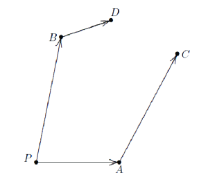
Figure 1: Schematic representation of an infinitesimal parallelogram. Here $(BD)^{\mu}=A^{\mu}-\Gamma^{\mu}_{\alpha\beta}(P)B^{\alpha}A^{\beta}$, while $(AC)^{\mu}=B^{\mu}-\Gamma^{\mu}_{\alpha\beta}(P)A^{\alpha}B^{\beta}$. Hence $(CD)^{\mu}=(\Gamma^{\mu}_{\alpha\beta}-\Gamma^{\mu}_{\beta\alpha})A^{\alpha}B^{\beta}$.

It is possible to introduce a coordinate system in the neighborhood of event $P$ such that the symmetric part of the connection vanishes BaMa ; that is, in the new system of coordinates $\Gamma^{\mu}_{(\alpha\beta)}(P)=0$. In this case, as depicted in Figure 2, $(CD)^{\mu}=2\delta^{\mu}$, where $\delta^{\mu}=\frac{1}{2}C_{\alpha\beta}{}^{\mu}(P)A^{\alpha}B^{\beta}$.

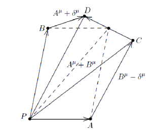
Figure 2: Schematic representation of the nonclosure of the parallelogram when $\Gamma^{\mu}_{(\alpha\beta)}(P)=0$..

It follows that in our extended GR framework, if the Weitzenböck torsion does not vanish at an event $P$, then infinitesimal parallelograms based at $P$ do not close. The situation is different, however, for non-infinitesimal parallelograms, whose closure, or lack thereof, would crucially depend on the detailed circumstances at hand and the nature of the spacetime under consideration.

V Concluding Remarks

Torsion, like curvature, is a basic tensor associated with a linear connection. The measurement of spacetime torsion depends upon the role that the torsion field plays in the physical theory. In the context of the Poincaré gauge theory of gravitation, for instance, Cartan’s torsion is related to intrinsic spin and the possibility of its measurement has been explored in that framework He ; La ; HOP . Another approach involves the motion of extended bodies in the context of nonminimal theories, where torsion couplings can be important PO .

Weitzenböck’s torsion has been previously studied in the context of teleparallelism MVRN ; MUF . In this paper, we have generalized previous work on the physical aspects of Weitzenböck’s torsion BaMa . In our extended GR framework, we have studied the general properties of this torsion field for orthonormal frames that are naturally adapted to static observers in gravitational fields. For the measured components of the torsion tensor, $C_{\hat{\alpha}\hat{\beta}}{}^{\hat{\gamma}}$, we find that $C_{\hat{0}\hat{i}}{}^{\hat{0}}$ represents what is essentially the gravitoelectric field, while $C_{\hat{i}\hat{j}}{}^{\hat{0}}$ represents what is essentially the gravitomagnetic field. Moreover, $C_{\hat{0}\hat{i}}{}^{\hat{j}}$ is related to the nonstationary character of the gravitational field and $C_{\hat{i}\hat{j}}{}^{\hat{k}}$ has in general mixed properties involving both the gravitoelectric and gravitomagnetic aspects. These results should be compared and contrasted with the frame components of the curvature tensor. Our work illustrates the fact that in the extended GR framework, curvature and torsion are complementary representations of the gravitational field.

Appendix A Nonsymmetric Connections

In our convention, the covariant derivative associated with a general nonsymmetric connection $\Gamma^{\mu}_{\alpha\beta}$ is defined for vector fields $A^{\mu}$ and $B_{\mu}$ as

$$\nabla_{\alpha}\,A^{\mu}=\partial_{\alpha}\,A^{\mu}+\Gamma^{\mu}_{\alpha\beta}\,A^{\beta}\,,\qquad\nabla_{\alpha}\,B_{\mu}=\partial_{\alpha}\,B_{\mu}-\Gamma^{\beta}_{\alpha\mu}\,B_{\beta}\,.$$ (66)

It follows that $\nabla_{\nu}\,e_{\mu}{}^{\hat{\alpha}}=0$ for the Weitzenböck connection. Furthermore, for a covariant vector field $A_{\mu}$,

$$\nabla_{\mu}\,A_{\nu}-\nabla_{\nu}\,A_{\mu}=\partial_{\mu}\,A_{\nu}-\partial_{\nu}\,A_{\mu}-C_{\mu\nu}{}^{\alpha}\,A_{\alpha}\,.$$ (67)

For a scalar field $S$, $\nabla_{\alpha}\,S=\partial_{\alpha}\,S$ and we have

$$(\nabla_{\alpha}\,\nabla_{\beta}-\nabla_{\beta}\,\nabla_{\alpha})\,S=C_{\alpha\beta}{}^{\mu}\,\partial_{\mu}\,S\,;$$ (68)

moreover, the Ricci identity takes the form

$$(\nabla_{\alpha}\,\nabla_{\beta}-\nabla_{\beta}\,\nabla_{\alpha})\,A_{\mu}=R^{\gamma}{}_{\mu\alpha\beta}A_{\gamma}+C_{\alpha\beta}{}^{\nu}\,\nabla_{\nu}\,A_{\mu}\,.$$ (69)

Here,

$$R^{\gamma}{}_{\mu\alpha\beta}=-R^{\gamma}{}_{\mu\beta\alpha}$$ (70)

is the curvature tensor given by

$$R^{\alpha}{}_{\mu\beta\nu}=\partial_{\beta}\,\Gamma^{\alpha}_{\nu\mu}-\partial_{\nu}\,\Gamma^{\alpha}_{\beta\mu}+\Gamma^{\alpha}_{\beta\sigma}\,\Gamma^{\sigma}_{\nu\mu}-\Gamma^{\alpha}_{\nu\sigma}\,\Gamma^{\sigma}_{\beta\mu}\,,$$ (71)

which vanishes in the case of Weitzenböck’s connection.

Appendix B Frame components of the Riemann tensor for static observers in the exterior Kerr spacetime

The symmetries of the Riemann curvature tensor make it possible to express its frame components ${}^{0}R_{\hat{\alpha}\hat{\beta}\hat{\gamma}\hat{\delta}}$ as elements of a symmetric $6\times 6$ matrix ${}^{0}{\mathcal{R}}=(^{0}{\mathcal{R}}_{IJ})$, where $I$ and $J$ range over the set $(01,02,03,23,31,12)$; that is,

$$^{0}{\mathcal{R}}=\left[\begin{array}[]{cc}{\hat{\mathcal{E}}}&{\hat{\mathcal{B}}}\cr{\hat{\mathcal{B}}}^{T}&{\hat{\mathcal{S}}}\cr\end{array}\right]\,,$$ (72)

where ${\hat{\mathcal{E}}}$ and ${\hat{\mathcal{S}}}$ are symmetric $3\times 3$ matrices and ${\hat{\mathcal{B}}}$ is traceless. Here ${\hat{\mathcal{E}}}$ and ${\hat{\mathcal{B}}}$ correspond to the gravitoelectric and gravitomagnetic components of spacetime curvature, respectively, while ${\hat{\mathcal{S}}}$ corresponds to its spatial components. In a Ricci-flat spacetime, ${\hat{\mathcal{S}}}=-{\hat{\mathcal{E}}}$, ${\hat{\mathcal{E}}}$ is traceless and ${\hat{\mathcal{B}}}$ is symmetric.

For the family of static observers in the exterior Kerr spacetime, the nonvanishing components of the symmetric and traceless ${\hat{\mathcal{E}}}=({\mathcal{E}}_{\hat{i}\hat{j}})$ and ${\hat{\mathcal{B}}}=({\mathcal{B}}_{\hat{i}\hat{j}})$ with respect to the frame (50)-(51) can be obtained from

$${\mathcal{E}}_{\hat{1}\hat{1}}=-\frac{Mr(r^{2}-3a^{2}\cos^{2}\theta)(2\Delta+a^{2}\sin^{2}\theta)}{\Sigma^{3}(\Sigma-2Mr)}\,,\quad{\mathcal{E}}_{\hat{1}\hat{2}}=-\frac{3Ma^{2}(3r^{2}-a^{2}\cos^{2}\theta)\sqrt{\Delta}\cos\theta\sin\theta}{\Sigma^{3}(\Sigma-2Mr)}\,,$$ (73)

$${\mathcal{E}}_{\hat{2}\hat{2}}=\frac{Mr(r^{2}-3a^{2}\cos^{2}\theta)(\Delta+2a^{2}\sin^{2}\theta)}{\Sigma^{3}(\Sigma-2Mr)}\,,\quad{\mathcal{E}}_{\hat{3}\hat{3}}=\frac{Mr}{\Sigma^{3}}(r^{2}-3a^{2}\cos^{2}\theta)\,$$ (74)

and

$${\mathcal{B}}_{\hat{1}\hat{1}}=\rho\,{\mathcal{E}}_{\hat{1}\hat{1}}\,,\quad{\mathcal{B}}_{\hat{1}\hat{2}}=\frac{1}{\rho}\,{\mathcal{E}}_{\hat{1}\hat{2}}\,,\quad{\mathcal{B}}_{\hat{2}\hat{2}}=\rho\,{\mathcal{E}}_{\hat{2}\hat{2}}\,,\quad{\mathcal{B}}_{\hat{3}\hat{3}}=\rho\,{\mathcal{E}}_{\hat{3}\hat{3}}\,,$$ (75)

where the dimensionless ratio $\rho$ is given by

$$\rho=\frac{a\cos\theta}{r}\left(\frac{3r^{2}-a^{2}\cos^{2}\theta}{r^{2}-3a^{2}\cos^{2}\theta}\right)\,.$$ (76)

We note that ${\hat{\mathcal{E}}}$ and ${\hat{\mathcal{B}}}$ diverge at the stationary limit $(g_{00}=0)$, and ${\hat{\mathcal{B}}}=0$ in the nonrotating Schwarzschild case, where $a=0$.

Appendix C Weitzenböck torsion invariants

Let $e_{\hat{\alpha}}$ be a given orthonormal frame and $C_{\hat{\alpha}\hat{\beta}}{}^{\hat{\gamma}}$ be the associated frame components of the structure functions. It is convenient to introduce the notation

$$C_{\hat{0}\hat{a}}{}^{\hat{0}}=\Psi_{\hat{a}}\,,\qquad C_{\hat{a}\hat{b}}{}^{\hat{0}}=\epsilon_{\hat{a}\hat{b}\hat{c}}W^{\hat{c}}\,,\qquad C_{\hat{0}\hat{a}}{}^{\hat{b}}=\chi_{\hat{a}}{}^{\hat{b}}\,.$$ (77)

Then, the torsion vector $C_{\hat{\alpha}}$ has components

$$C_{\hat{0}}=-\chi_{\hat{i}}{}^{\hat{i}}\,,\qquad C_{\hat{a}}=\Psi_{\hat{a}}-C_{\hat{a}\hat{b}}{}^{\hat{b}}\,;$$ (78)

while the torsion pseudovector $\check{C}_{\hat{\alpha}}$ has components

$$\check{C}_{\hat{0}}=-\frac{1}{6}\,\epsilon^{\hat{a}\hat{b}}{}_{\hat{c}}\,C_{\hat{a}\hat{b}}{}^{\hat{c}}\,,\qquad\check{C}_{\hat{a}}=\frac{1}{3}\,(W_{\hat{a}}-\epsilon_{\hat{a}\hat{b}\hat{c}}\,\chi^{\hat{b}\hat{c}})\,.$$ (79)

Next, we consider the three algebraic Weitzenböck invariants of the torsion tensor, namely,

$${\mathcal{I}}_{1}=C_{\hat{\alpha}\hat{\beta}}{}^{\hat{\gamma}}C^{\hat{\alpha}\hat{\beta}}{}_{\hat{\gamma}}\,,\qquad{\mathcal{I}}_{2}=C_{\hat{\alpha}\hat{\beta}\hat{\gamma}}C^{\hat{\gamma}\hat{\beta}\hat{\alpha}}\,,\qquad{\mathcal{I}}_{3}=C_{\hat{\alpha}}C^{\hat{\alpha}}\,.$$ (80)

In terms of the components of the torsion tensor, we have for ${\mathcal{I}}_{1}$ and ${\mathcal{I}}_{2}$

$${\mathcal{I}}_{1} = 2\Psi_{\hat{a}}\Psi^{\hat{a}}-2W_{\hat{a}}W^{\hat{a}}-2\chi_{\hat{a}\hat{b}}\,\chi^{\hat{a}\hat{b}}+C_{\hat{a}\hat{b}}{}^{\hat{c}}C^{\hat{a}\hat{b}}{}_{\hat{c}}\,,$$

$${\mathcal{I}}_{2} = \Psi_{\hat{a}}\Psi^{\hat{a}}-2\epsilon_{\hat{a}\hat{b}\hat{c}}\,W^{\hat{a}}\chi^{\hat{b}\hat{c}}-\chi_{\hat{a}\hat{b}}\,\chi^{\hat{b}\hat{a}}+C_{\hat{a}\hat{b}}{}^{\hat{c}}C_{\hat{c}}{}^{\hat{b}\hat{a}}\,.$$ (81)

Simplifications occur either in the case of the static Fermi observers, at the order of approximation employed in section II, or in the case of static observers in the general stationary axisymmetric spacetime considered in section III, since $\chi_{\hat{a}\hat{b}}=0$ in these cases.

References

• (1) R. Weitzenböck, Invariantentheorie (Noordhoff, Groningen, 1923).
• (2) Ll. Bel, “Connecting Connections”, arXiv:0805.0846 [gr-qc].
• (3) F. W. Hehl and B. Mashhoon, “Nonlocal Gravity Simulates Dark Matter”, Phys. Lett. B 673, 279 (2009). [arXiv: 0812.1059 [gr-qc]]
• (4) F. W. Hehl and B. Mashhoon, “Formal Framework for a Nonlocal Generalization of Einstein’s Theory of Gravitation”, Phys. Rev. D 79, 064028 (2009). [arXiv: 0902.0560 [gr-qc]]
• (5) S. Rahvar and B. Mashhoon, “Observational Tests of Nonlocal Gravity: Galaxy Rotation Curves and Clusters of Galaxies”, Phys. Rev. D 89, 104011 (2014). [arXiv:1401.4819 [gr-qc]]
• (6) B. Mashhoon, “Nonlocal Gravity: The General Linear Approximation”, Phys. Rev. D 90, 124031 (2014). [arXiv:1409.4472 [gr-qc]]
• (7) K. Hayashi and T. Shirafuji, “New General Relativity”, Phys. Rev. D 19, 3524 (1979).
• (8) M. Blagojević and F. W. Hehl, editors, Gauge Theories of Gravitation (Imperial College Press, London, 2013).
• (9) R. Aldrovandi and J. G. Pereira, Teleparallel Gravity: An Introduction (Springer, New York, 2013).
• (10) J. W. Maluf, “The Teleparallel Equivalent of General Relativity”, Ann. Phys. (Berlin) 525, 339 (2013). [arXiv: 1303.3897 [gr-qc]]
• (11) C. Møller, K. Dan. Vidensk. Selsk. Mat. Fys. Skr. 1, 10 (1961).
• (12) C. Pellegrini and J. Plebański, K. Dan. Vidensk. Selsk. Mat. Fys. Skr. 2, 4 (1963).
• (13) D. Bini, C. Chicone and B. Mashhoon, “Spacetime Splitting, Admissible Coordinates, and Causality”, Phys. Rev. D 85, 104020 (2012). [arXiv: 1203.3454 [gr-qc]]
• (14) B. Mashhoon, “The Hypothesis of Locality in Relativistic Physics”, Phys. Lett. A 145, 147 (1990).
• (15) J. L. Synge, Relativity: The General Theory (North-Holland, Amsterdam, 1971).
• (16) B. Mashhoon, Astrophys. J. 216, 591 (1977).
• (17) W.-T. Ni and M. Zimmermann, Phys. Rev. D 17, 1473 (1978).
• (18) C. Chicone and B. Mashhoon, Classical Quantum Gravity 19, 4231 (2002). [arXiv: gr-qc/0203073]
• (19) C. Chicone and B. Mashhoon, “Ultrarelativistic motion: Inertial and tidal effects in Fermi coordinates,” Classical Quantum Gravity 22, 195 (2005). [arXiv: gr-qc/0409017]
• (20) C. Chicone and B. Mashhoon, Phys. Rev. D 74, 064019 (2006). [arXiv: gr-qc/0511129]
• (21) A. Matte, Canadian J. Math. 5, 1 (1953).
• (22) R. T. Jantzen, P. Carini and D. Bini, Ann. Phys. (N.Y.)  215, 1 (1992). [arXiv: gr-qc/0106043]
• (23) B. Mashhoon, “Gravitoelectromagnetism: A Brief Review”, in The Measurement of Gravitomagnetism: A Challenging Enterprise, edited by L. Iorio (Nova Science, New York, 2007), Chap. 3, pp. 29–39. [arXiv:gr-qc/0311030]
• (24) B. Mashhoon, Galaxies 3, 1 (2015). [arXiv: 1411.5411 [gr-qc]]
• (25) F. W. Hehl, Phys. Lett. A 36, 225 (1971).
• (26) C. Lämmerzahl, Phys. Lett. A 228, 223 (1997). [arXiv: gr-qc/9704047]
• (27) F. W. Hehl, Yu. N. Obukhov and D. Puetzfeld, Phys. Lett. A 377, 1775 (2013). [arXiv:1304.2769 [gr-qc]]
• (28) D. Puetzfeld and Yu. N. Obukhov, Int. J. Mod. Phys. D 23, 1442004 (2014). [arXiv:1405.4137 [gr-qc]]
• (29) J. W. Maluf, M. V. O. Veiga and J. F. da Rocha-Neto, “Regularized Expression for the Gravitational Energy-Momentum in Teleparallel Gravity and the Principle of Equivalence”, Gen. Relativ. Gravit. 39, 227 (2007). [arXiv: gr-qc/0507122]
• (30) J. W. Maluf, S. C. Ulhoa and F. F. Faria, “Pound-Rebka Experiment and Torsion in the Schwarzschild Spacetime”, Phys. Rev. D 80, 044036 (2009). [arXiv: 0903.2565 [gr-qc]]