Trivariate polynomial approximation
on Lissajous curves  

Abstract

We study Lissajous curves in the 3-cube, that generate algebraic cubature formulas on a special family of rank-1 Chebyshev lattices. These formulas are used to construct trivariate hyperinterpolation polynomials via a single 1-d Fast Chebyshev Transform (by the Chebfun package), and to compute discrete extremal sets of Fekete and Leja type for trivariate polynomial interpolation. Applications could arise in the framework of Lissajous sampling for MPI (Magnetic Particle Imaging).

2010 AMS subject classification: 41A05, 41A10, 41A63, 65D05. Keywords: three-dimensional Lissajous curves, Lissajous sampling, Chebyshev lattices, trivariate polynomial interpolation and hyperinterpolation, discrete extremal sets.

1 Introduction

During the last decade, a new family of points for bivariate polynomial interpolation has been proposed and extensively studied, namely the so-called “Padua points” of the square; cf. [3, 5, 9, 10]. They are the first known optimal nodal set for total-degree multivariate polynomial interpolation, with a Lebesgue constant increasing like $(\log n)^{2}$, $n$ being the polynomial degree.

One of the key features of the Padua points, that has allowed to construct the interpolation formula, is that they lie on a suitable Lissajous curve, such that the integral of any polynomial of degree $2n$ along the curve is equal to the 2d-integral with respect to the product Chebyshev measure. More specifically, the Padua points are side contacts and self-intersections of the Lissajous curve.

Motivated by that construction, in the present paper we try to extend the Lissajous curve technique in dimension 3. Since the resulting curve is not self-intersecting, we cannot obtain total-degree polynomial interpolation. On the other hand, we are able to generate an algebraic cubature formula for the product Chebyshev measure, whose nodes lie on the Lissajous curve thus forming a rank-1 Chebyshev lattice (on Chebyshev lattices cf., e.g., [14]).

By such formula we can perform polynomial hyperinterpolation, which is a discretized orthogonal polynomial expansion [30], and can be constructed by a single 1-dimensional Fast Chebyshev Transform along the curve. Moreover, since the underlying Chebyshev lattices turn out to be Weakly Admissible Mehes for total-degree polynomials (cf. [7]), we can extract from them suitable discrete extremal sets of Fekete and Leja type for polynomial interpolation (cf. [6]). We provide a Matlab implementation of the hyperinterpolation and interpolation scheme, and show some numerical examples. Applications could arise within the emerging field of MPI (Magnetic Particle Imaging), cf. [25].

2 3d Lissajous curves and Chebyshev lattices

Below, we shall denote the product Chebyshev measure in $[-1,1]^{3}$ by

$$d\lambda=w(\boldsymbol{x})d\boldsymbol{x}\;,\;\;w(\boldsymbol{x})=\frac{1}{\sqrt{(1-x_{1}^{2})(1-x_{2}^{2})(1-x_{3}^{2})}}\;.$$ (1)

Moreover, $\mathbb{P}_{k}^{3}$ will denote the space of trivariate polynomials of degree not exceeding $k$, whose dimension is $\mbox{dim}(\mathbb{P}_{k}^{3})=(k+1)(k+2)(k+3)/6$.

Following the lines of the construction of the Padua points, the strategy adopted is to seek a Lissajous curve such that the integral of a polynomial in $\mathbb{P}_{2n}^{3}$ with respect to the Chebyshev measure $d\lambda$ is equal (up to a constant factor) to the integral of the polynomial along the curve. To this purpose, the following integer arithmetic result plays a key role.

Theorem 1

Let be $n\in\mathbb{N}^{+}$ and $(a_{n},b_{n},c_{n})$ be the integer triple

$$(a_{n},b_{n},c_{n})=\left\{\begin{array}[]{ll}\left(\frac{3}{4}n^{2}+\frac{1}{2}n,\frac{3}{4}n^{2}+n,\frac{3}{4}n^{2}+\frac{3}{2}n+1\right)\;,\;\;n\;\mbox{{\em even\/}}\\ \\ \left(\frac{3}{4}n^{2}+\frac{1}{4},\frac{3}{4}n^{2}+\frac{3}{2}n-\frac{1}{4},\frac{3}{4}n^{2}+\frac{3}{2}n+\frac{3}{4}\right)\;,\;\;n\;\mbox{{\em odd\/}}\end{array}\right.$$ (2)

Then, for ever integer triple $(i,j,k)$, not all $0$, with $i,j,k\geq 0$ and $i+j+k\leq m_{n}=2n$, we have the property that $ia_{n}\neq jb_{n}+kc_{n}$, $jb_{n}\neq ia_{n}+kc_{n}$, $kc_{n}\neq ia_{n}+jb_{n}$. Moreover, $m_{n}$ is maximal, in the sense that there exist a triple $(i^{\ast},j^{\ast},k^{\ast})$, $i^{\ast}+j^{\ast}+k^{\ast}=2n+1$, that does not satisfy the property.

Proof. See the Appendix.

Proposition 1

Consider the Lissajous curves in $[-1,1]^{3}$ defined by

$$\boldsymbol{\ell}_{n}(\theta)=(\cos(a_{n}\theta),\cos(b_{n}\theta),\cos(b_{n}\theta))\;,\;\;\theta\in[0,\pi]\;,$$ (3)

where $(a_{n},b_{n},c_{n})$ is the sequence of integer triples (2).

Then, for every total-degree polynomial $p\in\mathbb{P}_{2n}^{3}$

$$\int_{[-1,1]^{3}}{p(\boldsymbol{x})\,w(\boldsymbol{x})d\boldsymbol{x}}=\pi^{2}\,\int_{0}^{\pi}{p(\boldsymbol{\ell}_{n}(\theta))\,d\theta}\;.$$ (4)

Proof. It is sufficient to prove the identity for a polynomial basis. Take the total-degree product Chebyshev basis $T_{i}(x_{1})T_{j}(x_{2})T_{k}(x_{3})$, $i,j,k\geq 0$, $i+j+k\leq 2n$. For $i=j=k=0$, (4) is clearly true. For $i+j+k>0$, by orthogonality of the basis

$$\int_{[-1,1]^{3}}{T_{i}(x_{1})T_{j}(x_{2})T_{k}(x_{3})\,w(\boldsymbol{x})d\boldsymbol{x}}=0\;.$$

On the other hand,

$$\int_{0}^{\pi}{T_{i}(\cos(a_{n}\theta))T_{j}(\cos(b_{n}\theta))T_{k}(\cos(c_{n}\theta))\,d\theta}$$

$$=\int_{0}^{\pi}{\cos(ia_{n}\theta)\,\cos(jb_{n}\theta)\,\cos(kc_{n}\theta)\,d\theta}$$

$$=\frac{1}{4}\left\{\left.\left.\frac{\sin((ia_{n}-jb_{n}-kc_{n})\theta)}{ia_{n}-jb_{n}-kc_{n}}\right|_{0}^{\pi}+\frac{\sin((ia_{n}+jb_{n}-kc_{n})\theta)}{ia_{n}+jb_{n}-kc_{n}}\right|_{0}^{\pi}\right.$$

$$\left.\left.\left.+\frac{\sin((ia_{n}-jb_{n}+kc_{n})\theta)}{ia_{n}-jb_{n}+kc_{n}}\right|_{0}^{\pi}+\frac{\sin((ia_{n}+jb_{n}+kc_{n})\theta)}{ia_{n}+jb_{n}+kc_{n}}\right|_{0}^{\pi}\right\}$$

Now, the fourth summand on the right-hand side is zero since $ia_{n}+jb_{n}+kc_{n}>0$, and thus the whole right-hand side is zero if (and only if) $ia_{n}-jb_{n}-kc_{n}\neq 0$, $ia_{n}+jb_{n}-kc_{n}\neq 0$, $ia_{n}-jb_{n}+kc_{n}\neq 0$, which is true by Theorem 1 since $i+j+k\leq 2n$. $\;\;\;\square$

Corollary 1

Let be $p\in\mathbb{P}_{2n}^{3}$, $\boldsymbol{\ell}_{n}(\theta)$ the Lissajous curve (3) and

$$\nu=n\,\max\{a_{n},b_{n},c_{n}\}=\left\{\begin{array}[]{ll}\frac{3}{4}n^{3}+\frac{3}{2}n^{2}+n\;,\;\;n\;\mbox{{\em even\/}}\\ \\ \frac{3}{4}n^{3}+\frac{3}{2}n^{2}+\frac{3}{4}n\;,\;\;n\;\mbox{{\em odd\/}}\end{array}\right.$$ (5)

Then

$$\int_{[-1,1]^{3}}{p(\boldsymbol{x})\,w(\boldsymbol{x})d\boldsymbol{x}}=\sum_{s=0}^{\mu}{w_{s}\,p(\boldsymbol{\ell}_{n}(\theta_{s}))}\;,$$ (6)

where

$$w_{s}=\pi^{2}\omega_{s}\;,\;\;s=0,\dots,\mu\;,$$ (7)

with

$$\mu=\nu\;,\;\;\theta_{s}=\frac{(2s+1)\pi}{2\mu+2}\;,\;\;\omega_{s}\equiv\frac{\pi}{\mu+1}\;,\;\;s=0,\dots,\mu\;,$$ (8)

or alternatively

$$\mu=\nu+1\;,\;\;\theta_{s}=\frac{s\pi}{\mu}\;,\;\;s=0,\dots,\mu\;,$$

$$\omega_{0}=\omega_{\mu}=\frac{\pi}{2\mu}\;,\;\;\omega_{s}\equiv\frac{\pi}{\mu}\;,\;s=1,\dots,\mu-1\;.$$ (9)

Proof. Observe that by Proposition 1 and the change of variables $t=\cos(\theta)$

$$\int_{[-1,1]^{3}}{p(\boldsymbol{x})\,w(\boldsymbol{x})d\boldsymbol{x}}=\pi^{2}\,\int_{0}^{\pi}{p(\boldsymbol{\ell}_{n}(\theta))\,d\theta}$$

$$=\pi^{2}\,\int_{-1}^{1}{p(T_{a_{n}}(t),T_{b_{n}}(t),T_{c_{n}}(t))\,\frac{dt}{\sqrt{1-t^{2}}}}\;,$$

where $p(T_{a_{n}}(t),T_{b_{n}}(t),T_{c_{n}}(t))$ is a polynomial of degree not exceeding

$$2\nu=\max\{ia_{n}+jb_{n}+kc_{n}\,,\,i,j,k\geq 0\,,\,i+j+k\leq 2n\}=2n\,\max\{a_{n},b_{n},c_{n}\}\;.$$

The conclusion follows by using the classical Gauss-Chebyshev or Gauss-Chebyshev-Lobatto univariate quadrature rules, cf. (8) and (9) respectively, which are exact up to degree $2\nu+1$ using the $\mu+1$ nodes $\tau_{s}=\cos(\theta_{s})$ and weights $\omega_{s}$, cf., e.g., [26, Ch. 8].$\;\;\;\square$

Remark 1

(Chebyshev lattices). We observe that $\{\boldsymbol{\ell}_{n}(\theta_{s})\}$, $s=0,\dots,\mu$, are 3-dimensional rank-1 Chebyshev lattices (for cubature degree of exactness $2n$) in the terminology of [14]. As opposite to [15], where Chebsyhev lattices are generated heuristically by a search algorithm, here we have a formula to generate rank-1 Chebyshev lattices for any degree.

2.1 Optimal Tuples and Homogeneous Diophantine Equations

An algebraic trivariate polynomial of degree $N$ restricted to the Lissajou curve $\boldsymbol{\ell}_{n}(\theta)$ is a trigonometric polynomial of degree $N\max\{a_{n},b_{n},c_{n}\}=Nc_{n}.$ Hence it is some interest to have a triple for which the conclusion of Theorem 1 holds with its maximum as small as possible. Indeed, we conjecture that the triples (2) are optimal in this sense.

Conjecture 1

Suppose that $(a,b,c)$ is a triple of strictly positive integers such that $\max\{a,b,c\}<c_{n},$ with $c_{n}$ given by (2). Then there exists an integer triple $(i,j,k),$ not all $0,$ and $i+j+k\leq 2n$, such that either $ia=jb+kc$, $jb=ia+kc$, or $kc=ia+jb$. In other words, the triples (2) are those satisfying the conclusion of Theorem 1 having the minimum maximum.

We do not as yet have a proof of this conjecture but can provide a lower bound for the minimum maximum of such “good” triples with the correct order of growth in $n.$

First observe that the conditions of the conclusion of Theorem 1 may be expressed more succinctly in terms of a homogeneous linear Diophantine equation.

Lemma 1

Suppose that $(a,b,c)$ is a triple of strictly positive integers. Then there exists an integer triple $(i,j,k),$ not all $0,$ and $i+j+k\leq N$, such that either $ia=jb+kc$, $jb=ia+kc$, or $kc=ia+jb$ iff there exists an integer triple $(x,y,z)\in\mathbb{Z}^{3}$ such that $|x|+|y|+|z|\leq N$ and $xa+yb+zc=0.$

Proof. If, for example, $ia=jb+kc,$ then $-ia+jb+kc=0$ and we may take $x=-i,$ $y=j$ and $z=k.$ On the other hand, if $xa+yb+zc=0$ then not all of $x,$ $y$ and $z$ can have the same sign. There being an odd number of them, two of them have the same sign and the other the opposite sign. By multiplying by $-1$ if necessary, we assume that the single sign is negative. For example, if it is $x$ that is negative, we may write $-xa=yb+zc$ and take $i=-x,$ $j=y$ and $k=z.$ $\;\;\;\square$

The classical Siegel’s Lemma (see e.g. [34, p. 168]) gives a bound on the order of growth of “small” solutions of homogeneous linear diophantine equations. We may adapt this to our situation to prove

Lemma 2

(A version of Siegel’s Lemma) Suppose that $1\leq n\in\mathbb{Z}_{+}.$ Suppose further that $a=[a_{1},a_{2},\ldots,a_{d}]\in\mathbb{Z}_{+}^{d}$ with $a_{i}>0,$ $1\leq i\leq d,$ is such that

$$\max\{a\}\leq M$$

where

$$M:=\left\lfloor\frac{1}{n}{n+d\choose d}\right\rfloor-2\quad(=O(n^{d-1})).$$

Then there exists $0\neq x\in\mathbb{Z}^{d}$ such that $\sum_{i=1}^{d}|x_{i}|\leq 2n$ and

$$\sum_{i=1}^{d}x_{i}a_{i}=0.$$

Proof. Let $S_{d}\subset\mathbb{Z}_{+}^{d}$ denote the set of positive tuples $0\neq z\in\mathbb{Z}_{+}^{d}$ such that $\sum_{i=1}^{d}z_{i}\leq n.$ Then $\#(S_{d})={n+d\choose d}-1.$

Consider the map $F\,:\,\mathbb{Z}^{d}\to\mathbb{Z}$ given by

$$F(z):=\sum_{i=1}^{d}a_{i}z_{i}.$$

Then $F(S_{d})\subset[1,nM]$ and hence

$$\#(F(S_{d}))\leq nM.$$

But

$$nM=n\left\{\left\lfloor\frac{1}{n}{n+d\choose n}\right\rfloor-2\right\}\leq{n+d\choose d}-2n<{n+d\choose d}-1,$$

i.e.,

$$\#(F(S_{d}))<\#(S_{d}).$$

It follows from the Pigeon Hole Principle that there exists two different tuples $y^{(1)}\neq y^{(2)}\in S_{d}$ such that

$$F(y^{(1)})=F(y^{(2)}),$$

i.e.,

$$\sum_{i=1}^{d}a_{i}(y_{i}^{(1)}-y_{i}^{(2)})=0.$$

The tuple $x:=y^{(1)}-y^{(2)}$ has the desired properties. $\;\;\;\square$

In our context it means that the minimum maximum of “good” tuples is at least

$$M:=\left\lfloor\frac{1}{n}{n+d\choose d}\right\rfloor-2\quad(=O(n^{d-1})).$$

3 Hyperinterpolation on Lissajous curves

We shall adopt the following notation. We denote the total-degree orthonormal basis of $P_{n}^{3}([-1,1]^{3})$ with respect to the Chebyshev product measure (1) by

$$\hat{\phi}_{i,j,k}(\boldsymbol{x})=\hat{T_{i}}(x_{1})\hat{T_{j}}(x_{2})\hat{T_{k}}(x_{3})\;,\;i,j,k\geq 0\;,\;i+j+k\leq n\;,$$ (10)

where $\hat{T}_{m}(\cdot)$ is the normalized Chebyshev polynomial of degree $m$

$$\hat{T}_{m}(\cdot)=\sigma_{m}\cos(m\arccos(\cdot))\;,\;\;\sigma_{m}=\sqrt{\frac{1+\mbox{sign}(m)}{\pi}}\;,\;\;m\geq 0\;,$$ (11)

with the convention that $\mbox{sign}(0)=0$.

We recall that hyperinterpolation is a discretized expansion of a function in series of orthogonal polynomials up to total-degree $n$ on a given $d$-dimensional compact region $K$, where the Fourier-like coefficients are computed by a cubature formula exact on $\mathbb{P}^{d}_{2n}(K)$. It was proposed by Sloan in the seminal paper [30] in order to bypass the intrinsic difficulties of polynomial interpolation in the multivariate setting, and since then has been successfully used in several instances, for example on the sphere [24].

Given a function $f\in C([-1,1]^{3})$, in view of the algebraic cubature formula (6), the hyperinterpolation polynomial of $f$ is

$$\mathcal{H}_{n}f(\boldsymbol{x})=\sum_{0\leq i+j+k\leq n}{C_{i,j,k}\,\hat{\phi}_{i,j,k}(\boldsymbol{x})}\;,$$ (12)

where

$$C_{i,j,k}=\sum_{s=0}^{\mu}{w_{s}\,f(\boldsymbol{\ell}_{n}(\theta_{s}))\,\hat{\phi}_{i,j,k}(\boldsymbol{\ell}_{n}(\theta_{s}))}\;.$$ (13)

Observe that by construction $\mathcal{H}_{n}f=f$ for every $f\in\mathbb{P}_{n}^{3}$, i.e., $\mathcal{H}_{n}$ is a projection operator. Among the properties of the hyperinterpolation operator, not depending on the specific cubature formula provided it is exact up to degree $2n$ for the product Chebyshev measure, we recall the following bound for the $L^{2}$ error,

$$\|f-\mathcal{H}_{n}f\|_{2}\leq 2\pi^{3}\,E_{n}(f)\;,\;\;E_{n}(f)=\inf_{p\in\mathbb{P}_{n}}\|f-p\|_{\infty}\;.$$ (14)

Consider the uniform operator norm (i.e., the Lebesgue constant)

$$\|\mathcal{H}_{n}\|=\sup_{f\neq 0}\frac{\|\mathcal{H}_{n}f\|_{\infty}}{\|f\|_{\infty}}=\max_{\boldsymbol{x}\in[-1,1]^{3}}{\sum_{s=0}^{\mu}{w_{s}\,\left|K_{n}(\boldsymbol{x},\boldsymbol{\ell}_{n}(\theta_{s}))\right|}}\;,$$ (15)

where $K_{n}(\boldsymbol{x},\boldsymbol{y})=\sum_{0\leq i+j+k\leq n}{\hat{\phi}_{i,j,k}(\boldsymbol{x})\hat{\phi}_{i,j,k}(\boldsymbol{y})}$ is the reproducing kernel of $\mathbb{P}_{n}^{3}$ with respect to the product Chebyshev measure (1), cf. [22].

In [17] the bound $\|\mathcal{H}_{n}\|=\mathcal{O}((\sqrt{n})^{3})$ has been obtained, as a consequence of a general result connecting multivariate Christoffel functions and hyperinterpolation operator norms. On the other hand, by proving a conjecture stated in [20], the fine bound

$$\|\mathcal{H}_{n}\|=\mathcal{O}((\log n)^{3})$$ (16)

has been provided in [35], which corresponds to the minimal growth of a polynomial projection operator, in view of [32]. Since $\mathcal{H}_{n}$ is a projection, we get the $L^{\infty}$ error bound

$$\|f-\mathcal{H}_{n}f\|_{\infty}=\mathcal{O}\left((\log n)^{3}\,E_{n}(f)\right)\;.$$ (17)

We show now that the hyperinterpolation coefficients $\{C_{i,j,k}\}$ can be computed by a single 1-dimensional discrete Chebyshev transform along the Lissajous curve.

Proposition 2

Let be $f\in C([-1,1]^{3})$, $(a_{n},b_{n},c_{n})$ the sequence of integer triples (2), and $\nu$, $\mu$, $\{\theta_{s}\}$, $\omega_{s}$, $\{w_{s}\}$ as in Corollary 1. The hyperinterpolation coefficients of $f$ generated by (6) can be computed as

$$C_{i,j,k}=\frac{\pi^{2}}{4}\,\sigma_{ia_{n}}\sigma_{jb_{n}}\sigma_{kc_{n}}\,\left(\frac{\gamma_{\alpha_{1}}}{\sigma_{\alpha_{1}}}+\frac{\gamma_{\alpha_{2}}}{\sigma_{\alpha_{2}}}+\frac{\gamma_{\alpha_{3}}}{\sigma_{\alpha_{3}}}+\frac{\gamma_{\alpha_{4}}}{\sigma_{\alpha_{4}}}\right)\;,$$ (18)

$$\alpha_{1}=ia_{n}+jb_{n}+kc_{n}\;,\;\;\alpha_{2}=\left|ia_{n}+jb_{n}-kc_{n}\right|\;,$$

$$\alpha_{3}=\left|ia_{n}-jb_{n}\right|+kc_{n}\;,\;\;\alpha_{4}=\left|\left|ia_{n}-jb_{n}\right|-kc_{n}\right|\;,$$

where $\{\gamma_{m}\}$ are the first $\nu+1$ coefficients of the discretized Chebyshev expansion of $f(T_{a_{n}}(t),T_{b_{n}}(t),T_{c_{n}}(t))$, $t\in[-1,1]$, namely

$$\gamma_{m}=\sum_{s=0}^{\mu}{\omega_{s}\,\hat{T}_{m}(\tau_{s})\,\,f(T_{a_{n}}(\tau_{s}),T_{b_{n}}(\tau_{s}),T_{c_{n}}(\tau_{s}))}\;,$$ (19)

$m=0,1,\dots,\nu$, with $\tau_{s}=\cos(\theta_{s})$, $s=0,1,\dots,\mu$.

Proof. By the change of variables $\theta=\arccos(t)$ which gives

$$\boldsymbol{\ell}_{n}(\theta)=(T_{a_{n}}(t),T_{b_{n}}(t),T_{c_{n}}(t))\;,$$

and by the classical identity $T_{h}(t)T_{k}(t)=\frac{1}{2}\,\left(T_{h+k}(t)+T_{|h-k|}(t)\right)$ (cf., e.g., [26, §2.4.3]), we get

$$f(\boldsymbol{\ell}_{n}(\theta))\,\hat{\phi}_{i,j,k}(\boldsymbol{\ell}_{n}(\theta))=f(\boldsymbol{\ell}_{n}(\arccos(t)))\,\,\hat{T}_{ia_{n}}(t)\hat{T}_{jb_{n}}(t)\hat{T}_{kc_{n}}(t)$$

$$=f(\boldsymbol{\ell}_{n}(\arccos(t)))\,\sigma_{ia_{n}}\sigma_{jb_{n}}\sigma_{kc_{n}}\,\frac{1}{4}\,\left(T_{\alpha_{1}}(t)+T_{\alpha_{2}}(t)+T_{\alpha_{3}}(t)+T_{\alpha_{4}}(t)\right)\;,$$

and hence we have (18)-(19) in view of (13), and the fact that $\{\tau_{s}\}$ are the nodes of the univariate Gauss-Chebyshev or Gauss-Chebyshev-Lobatto formula, with weights $\omega_{s}$, cf. (8)-(9). $\;\;\;\square$

Remark 2

(Lissajous sampling). Hyperinterpolation polynomials on $d$-dimensional cubes can be constructed by other cubature formulas for the product Chebyshev measure, that can be more efficient in terms of number of function evaluations required at a given exactness degree. For example, a formula of exactness degree $2n$ with $\mathcal{O}(n^{4})$ nodes for the 3-cube has been provided in [20], and used in a FFT-based implementation of hyperinterpolation. Other formulas, in particular Godzina’s blending formulas [23], that have the lowest cardinality known in $d$-dimensional cubes, have been used in the package [16]. All such formulas are based on Chebyshev lattices of rank greater than 1, that are suitable unions of product Chebyshev subgrids.

A first advantage of rank-1 Chebyshev lattices, as observed in general in [14], is that a single 1-dimensional FFT is needed to compute the hyperinterpolation polynomials. In the present context of sampling on Lissajous curves of the 3-cube, this is manifest in Proposition 2.

On the other hand, one of the most most interesting features of hperinterpolation on Lissajous curves arises in connection with medical imaging applications, in particular with the emerging 3d MPI (Magnetic Particle Imaging) technology. Indeed, Lissajous sampling is one of the most common sampling methods within this technology, since it can be generated by suitable electromagnetic fields with different frequencies in the components, cf., e.g., [25, 28]. Choosing the frequencies (2) that generate the specific 3d Lissajous curves (3), a clear connection with multivariate polynomial approximation comes out, that could be useful in the corresponding data processing and analysis.

Remark 3

(Clenshaw-Curtis type cubature). The availability of an hyperinterpolation operator with respect to a given density function (here the trivariate Chebyshev density) allows us to easily construct algebraic cubature formulas for other densities, generalizing the Clenshaw-Curtis quadrature approach (cf., e.g., [26]). Indeed, if the “moments”

$$m_{i,j,k}=\int_{[-1,1]^{3}}{\hat{\phi}_{i,j,k}(\boldsymbol{x})\,\xi(\boldsymbol{x})d\boldsymbol{x}}\;,\;\;i,j,k\geq 0\;,\;\;i+j+k\leq n$$ (20)

are known, where $\xi\in L^{1}_{+}((-1,1)^{3})$, as shown in [31] we can construct by (13) the cubature formula

$$\int_{[-1,1]^{3}}{\mathcal{H}_{n}f(\boldsymbol{x})\,\xi(\boldsymbol{x})d\boldsymbol{x}}=\sum_{0\leq i+j+k\leq n}{C_{i,j,k}\,m_{i,j,k}}$$

$$=\sum_{s=0}^{\mu}{W_{s}\,f(\boldsymbol{\ell}_{n}(\theta_{s}))}\;,\;\;W_{s}=w_{s}\,\sum_{0\leq i+j+k\leq n}{m_{i,j,k}\,\hat{\phi}_{i,j,k}(\boldsymbol{\ell}_{n}(\theta_{s}))}\;,$$ (21)

which is exact for all polynomials in $\mathbb{P}_{n}^{3}$. The resulting weights $\{W_{s}\}$ are not all positive, in general, but if $\xi/w\in L^{2}((-1,1)^{3})$, which is true for example for the Lebesgue measure $\xi(\boldsymbol{x})\equiv 1$, it can be proved that

$$\lim_{n\to\infty}{\sum_{s=0}^{\mu}{|W_{s}|}}=\int_{[-1,1]^{3}}{\frac{\xi(\boldsymbol{x})}{w(\boldsymbol{x})}\,d\boldsymbol{x}}\;,$$ (22)

thus ensuring convergence and stability of the cubature formula; cf. [31].

We stress that these Clenshaw-Curtis type cubature formulas are based on Lissajous sampling (see Remark 2), and by Proposition 2 can be constructed by a single 1-dimensional discrete Chebyshev transform along the Lissajous curve (i.e., by a single 1-dimensional FFT).

Remark 4

(Weakly Admissible Meshes and Discrete Extremal Sets). In the recent literature on multivariate polynomial approximation, the notion of “Weakly Admissible Mesh” has emerged as a basic tool, from both the theoretical and the computational point of view; cf., e.g., [6, 7, 11] and the references therein.

We recall that a Weakly Admissible Mesh (WAM) is a sequence of finite subsets of a multidimensional (polynomial-determining) compact set, say $\mathcal{A}_{n}\subset K\subset\mathbb{R}^{d}$ (or $\mathbb{C}^{d}$), which are norming sets for total-degree polynomial subspaces,

$$\|p\|_{\infty,K}\leq C(\mathcal{A}_{n})\,\|p\|_{\infty,\mathcal{A}_{n}}\;,\;\;\forall p\in\mathbb{P}_{n}^{d}\;,$$ (23)

where both $C(\mathcal{A}_{n})$ and $\mbox{card}(\mathcal{A}_{n})$ increase at most polynomially with $n$. Here, $\mathbb{P}_{n}^{d}$ denotes the space of $d$-variate polynomials of degree not exceeding $n$, and $\|f\|_{\infty,X}$ the sup-norm of a function $f$ bounded on the (discrete or continuous) set $X$. Observe that necessarily $\mbox{card}(\mathcal{A}_{n})\geq\mbox{dim}(\mathbb{P}_{n}^{d})$.

Among their properties, we quote that WAMs are preserved by affine transformations, can be constructed incrementally by finite union and product, and are “stable” under small perturbations [29]. It has been shown in the seminal paper [11] that WAMs are nearly optimal for polynomial least-squares approximation in the uniform norm. Moreover, the interpolation Lebesgue constant of Fekete-like extremal sets extracted from such meshes, say $\mathcal{F}_{n}$ (that are points maximizing the Vandermonde determinant on $\mathcal{A}_{n}$), has the bound

$$\Lambda(\mathcal{F}_{n})\leq\mbox{dim}(\mathbb{P}_{n}^{d})\,C(\mathcal{A}_{n})\;.$$ (24)

Now, the Chebyshev lattices

$$\mathcal{A}_{n}=\{\boldsymbol{\ell}_{n}(\theta_{s})\,,\,\,s=0,\dots,\mu\}$$ (25)

in (8)-(9), form a WAM for $K=[-1,1]^{3}$, with $C(\mathcal{A}_{n})=\mathcal{O}((\log n)^{3})$. In fact, the corresponding hyperinterpolation operator $\mathcal{H}_{n}$ being a projection on $\mathbb{P}_{n}^{3}$, we get by (16)

$$\|p\|_{\infty,[-1,1]^{3}}=\|\mathcal{H}_{n}p\|_{\infty,[-1,1]^{3}}\leq\|\mathcal{H}_{n}\|\,\|p\|_{\infty,\mathcal{A}_{n}}=\mathcal{O}((\log n)^{3})\,\|p\|_{\infty,\mathcal{A}_{n}}\;.$$ (26)

In the next Section, we shall use the fact that Fekete-like extremal sets extracted from $\mathcal{A}_{n}=\{\boldsymbol{\ell}_{n}(\theta_{s})\,,\,\,s=0,\dots,\mu\}$ provide a Lissajous sampling approach to trivariate polynomial interpolation.

4 Implementation and numerical examples

4.1 Hyperinterpolation by Lissajous sampling

In view of Proposition 2, hyperinterpolation on the Lissajous curve can be implemented by a single 1-dimensional Discrete Chebyshev Transform, i.e., by a single 1-dimensional FFT. We shall concentrate on sampling at the Chebyshev-Lobatto points, since in this case we can conveniently resort to the powerful Chebfun package (cf. [21]). Sampling at the Chebyshev zeros can be treated in a similar way.

Indeed, in view of a well-known discrete orthogonality property of the Chebyshev polynomials, the interpolation polynomial of a function $g$ at the Chebyshev-Lobatto points can be written as

$$\pi_{\mu}(t)=\sum_{m=0}^{\mu}{c_{m}T_{m}(t)}$$ (27)

where

$$c_{m}=\frac{2}{\mu}\,\sum_{s=0}^{\mu}{{}^{\prime\prime}\,T_{m}(\tau_{s})\,g(\tau_{s})}\;,\;\;m=1,\dots,\mu-1\;,$$

$$c_{m}=\frac{1}{\mu}\,\sum_{s=0}^{\mu}{{}^{\prime\prime}\,T_{m}(\tau_{s})\,g(\tau_{s})}\;,\;\;m=0,\mu\;,$$ (28)

the double prime indicating that the first and the last terms of the sum have to be halved (cf., e.g., [26, §6.3.2]).

Applying this interpolation formula to $g(t)=f(T_{a_{n}}(t),T_{b_{n}}(t),T_{c_{n}}(t))$ and comparing with the discrete Chebyshev expansion coefficients (19), we obtain by easy calculations

$$\frac{\gamma_{m}}{\sigma_{m}}=\left\{\begin{array}[]{ll}\frac{\pi}{2}\,c_{m}\;,\;\;m=1,\dots,\mu-1\\ \\ \pi\,c_{m}\;,\;\;m=0,\mu\end{array}\right.$$ (29)

i.e., the 3-dimensional hyperinterpolation coefficients (18) can be computed by the $\{c_{m}\}$ and (29).

The coefficients of Chebyshev-Lobatto interpolation (28) are at the core of the Chebfun package, cf. [1, 33]. A single call to the Chebfun basic function chebfun on $f(T_{a_{n}}(t),T_{b_{n}}(t),T_{c_{n}}(t))$, truncated at the $(\mu+1)$th-term, produces all the relevant coefficients $\{c_{m}\}$ in an extremely fast and stable way.

For example, by the Matlab code [19] we can compute in about 1 second the $\mu=\frac{3}{4}n^{3}+\frac{3}{2}n^{2}+n+2=765102$ coefficients for $n=100$ with functions such as

$$f_{1}(\boldsymbol{x})=\exp(-c\|\boldsymbol{x}\|_{2}^{2})\;,\;c>0\;,\;\;f_{2}(\boldsymbol{x})=\|\boldsymbol{x}\|_{2}^{\beta}\;,\;\beta>0\;,$$ (30)

from which we get by (18) the $(n+1)(n+2)(n+3)/6=176851$ coefficients of trivariate hyperinterpolation at degree $n=100$. All the numerical tests have been made by Chebfun 5.1, in Matlab 7.7.0 with an Athlon 64 X2 Dual Core 4400+ 2.40GHz processor.

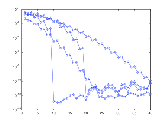
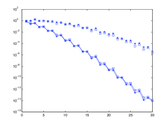
For the purpose of illustration, in Figure 1 we show the relative errors (in the Euclidean norm on a suitable control grid) for two polynomials of degree 10 and 20, respectively, and for the test functions $f_{1}$ and $f_{2}$ in (30). Observe the Gaussian $f_{1}$ is analytic, with variation rate determined by the parameter $c$, whereas the power function $f_{2}$ has finite regularity, determined by the parameter $\beta$.

Notice that the error decreases with the degree to a certain threshold above machine precision and thereafter does not improve. This is likely due to the fact that we require the summation of a large number of terms, for which a non-negligible error is to be expected. For practical applications this is of little import.

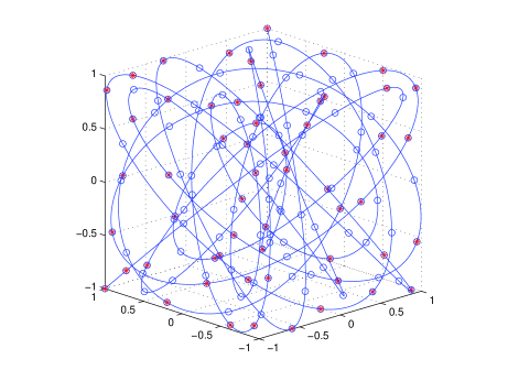
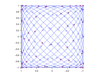
In Figures 2 and 3 one can see the Chebyshev lattice on the Lissajous curve for polynomial degree $n=5$.

Figure 1: Top: Hyperinterpolation errors for the trivariate polynomials $\|\boldsymbol{x}\|_{2}^{2k}$ with $k=5$ (diamonds) and $k=10$ (triangles), and for the trivariate function $f_{1}$ with $c=1$ (squares) and $c=5$ (circles). Bottom: Hyperinterpolation errors for the trivariate function $f_{2}$ with $\beta=5$ (squares) and $\beta=3$ (circles).

4.2 Interpolation by Lissajous sampling

Concerning polynomial interpolation in the cube by sampling on the Lissajous curve, we resort to the approximate versions of Fekete points (points that maximize the absolute value of the Vandermonde determinant) studied in several recent papers [4, 6, 32]. By (24), it makes sense to start from a WAM, namely the Chebyshev lattice $\mathcal{A}_{n}$ in (25), by the corresponding Vandermonde-like matrix

$$V=V(\mathcal{A}_{n};\boldsymbol{\phi})\in\mathbb{R}^{M\times N}\;,\;\;M=\mbox{card}(\mathcal{A}_{n})=\mu+1\;,\;\;N=\mbox{dim}(\mathbb{P}_{n}^{3})\;,$$ (31)

(cf. (8)-(9) for the definition of $\mu$), where

$$\boldsymbol{\phi}=\{\phi_{i,j,k}\}\;,\;\;\phi_{i,j,k}(\boldsymbol{x})=T_{i}(x_{1})T_{j}(x_{2})T_{k}(x_{3})\;,\;\;0\leq i+j+k\leq n\;,$$

is the total-degree trivariate Chebyshev orthogonal basis, suitably ordered (we adopt the graded lexicographical ordering, that is the lexicographical ordering within each subset of triples $(i,j,k)$ such that $i+j+k=r$, $r=0,\dots,n$). The $(p,q)$ entry of $V$ is the $q$-th element of the ordered basis computed in the $p$-th element of the nodal array. We recall that the choice of the Chebyshev orthogonal basis allows to avoid the extreme ill-conditiong of Vandermonde matrices in the standard monomial basis.

The problem of selecting a $N\times N$ square submatrix with maximal determinant from a given $M\times N$ rectangular matrix is known to be NP-hard [13], but can be solved in an approximate way by two simple greedy algorithms, that are fully described and analyzed in [6]. These algorithms produce two interpolation nodal sets, called discrete extremal sets.

The first, that computes the so-called Approximate Fekete Points (AFP), tries to maximize iteratively submatrix volumes until a maximal volume $N\times N$ submatrix of $V$ is obtained, and can be based on the famous QR factorization with column pivoting [8], applied to $V^{t}$ (that in Matlab is implemented by the matrix left division or backslash operator, cf. [27]). See [13] for the notion of volume generated by a set of vectors, which generalizes the geometric concept related to parallelograms and parallelepipeds (the volume and determinant notions coincide on a square matrix).

The second, that computes the so-called Discrete Leja Points (DLP), tries to maximize iteratively submatrix determinants, and is based simply on Gaussian elimination with row pivoting applied to the Vandermonde-like matrix $V$.

Denoting by $A$ the $M\times 2$ array of the WAM nodal coordinates, the corresponding computational steps, written in a Matlab-like style, are

$$\boldsymbol{w}=V\backslash\boldsymbol{v};\;\boldsymbol{s}={\tt find}(\boldsymbol{w}\neq\boldsymbol{0});\;\mathcal{F}_{n}^{\small{AFP}}=A(\boldsymbol{s},:);$$ (32)

for AFP, where $\boldsymbol{v}$ is any nonzero $N$-dimensional vector, and

$$[L,U,\boldsymbol{\sigma}]={\tt LU}(V,``{\tt vector}");\;\boldsymbol{s}=\boldsymbol{\sigma}(1:N);\;\mathcal{F}_{n}^{\small{DLP}}=A(\boldsymbol{s},:);$$ (33)

for DLP. In (33), we refer to the Matlab version of the LU factorization that produces a row permutation vector. In both algorithms, we eventually select an index subset $\boldsymbol{s}=(s_{1},\dots,s_{N})$, that extracts a Fekete-like discrete extremal set $\mathcal{F}_{n}$ of the cube from the WAM $\mathcal{A}_{n}$.

Once the underlying extraction WAM has been fixed, differently from the continuum Fekete points, Approximate Fekete Points depend on the choice of the basis, and Discrete Leja Points depend also on its order. An important feature is that Discrete Leja Points form a sequence, i.e., if the polynomial basis is such that its first $N_{r}=\mbox{dim}(\mathbb{P}^{d}_{r})$ elements span $\mathbb{P}^{d}_{r}$, $1\leq r\leq n$ (as it happens with the graded lexicographical ordering of the Chebyshev basis), then the first $N_{r}$ Discrete Leja Points are a unisolvent set for interpolation in $\mathbb{P}^{d}_{r}$.

Under the latter assumption for Discrete Leja Points, the two families of discrete extremal sets share the same asymptotic behavior, which by a recent deep result in pluripotential theory, cf. [2], is exactly that of the continuum Fekete points: the corresponding uniform discrete probability measures converge weakly to the pluripotential theoretic equilibrium measure of the underlying compact set, cf. [4, 6]. In the present case of the cube, such a measure is the product Chebyshev measure (1), with scaled density $w(\boldsymbol{x})/\pi^{3}$.

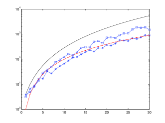
We give now some numerical examples, that can be reproduced by the Matlab package [18]. First, in Figures 2-3 we show the Approximate Fekete Points extracted from the Chebyshev lattice on the Lissajous curve for degree $n=5$. In Figure 4 we display the numerically evaluated Lebesgue constants of the Approximate Fekete Points and Discrete Leja Points for degree $n=1,2,\dots,30$. For both the nodal families, the Lebesgue constant turns out to be much lower than the upper bound (24), and even lower than $N=\mbox{dim}(\mathbb{P}_{n}^{3})$, a theoretical upper bound for the continuum Fekete points. In particular, the Lebesgue constant of Approximate Fekete Points seems to increase quadratically with respect to the degree, at least in the given degree range.

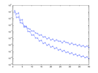
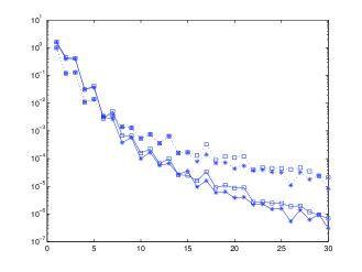
Finally, In Figure 5 we show the relative interpolation errors for the two test functions $f_{1}$ and $f_{2}$ of Figure 1. Since the Discrete Leja Points form a sequence, as discussed above, we have computed them once and for all for degree $n=30$, and then used the nested subsequences with $N_{r}=\mbox{dim}(\mathbb{P}^{d}_{r})$ elements for interpolation at degree $r=1,\dots,30$. The corresponding file of nodal coordinates can be downloaded from [18]. The relevant indexes $(s_{1},s_{2},\dots,s_{N_{30}})$ corresponding to the extraction of the Discrete Leja Points from the Chebyshev lattice (25)-(9) at degree 30, could be used in applications, such as MPI [25], where a trivariate function is not known or computable everywhere, but can be sampled just by travelling along the Lissajous curve.

Figure 2: The Chebyshev lattice (circles) and the extracted Approximate Fekete Points (asterisks), on the Lissajous curve for polynomial degree $n=5$.

Figure 3: A face projection of the Lissajous curve above with the sampling nodes.

Figure 4: Lebesgue constants (log scale) of the Approximate Fekete Points (asterisks) and Discrete Leja Points (squares) extracted from the Chebyshev lattices on the Lissajous curves, for degree $n=1,2,\dots,30$, compared with $\mbox{dim}(\mathbb{P}_{n}^{3})=(n+1)(n+2)(n+3)/6$ (upper solid line) and $n^{2}$ (dots).

Figure 5: Interpolation errors on Approximate Fekete Points (asterisks) and Discrete Leja Points (squares) for the trivariate functions $f_{1}$ (top) with $c=1$ (solid line) and $c=5$ (dotted line), and $f_{2}$ (bottom) with $\beta=5$ (solid line) and $\beta=3$ (dotted line).

5 Appendix

Proof of Theorem 1. We prove the theorem for $n$ even, the proof being similar in the odd case. Let be $m=n/2$, $n$ even, so that

$$(a_{n},b_{n},c_{n})=(3m^{2}+m,3m^{2}+2m,3m^{2}+3m+1)\;.$$

We assume that

$$i^{2}+j^{2}+k^{2}>0\;.$$

First case. We show that it is not possible to have

$$ia=jb+kc$$

for $i+j+k\leq 4m$ $(=2n)$. Now, $ia=jb+kc$ becomes $i(3m^{2}+m)+j(3m^{2}+2m)+k(3m^{2}+3m)+k$. Since $m$ divides $3m^{2}+m$, $3m^{2}+2m$ and $3m^{2}+3m$, we must have that $m$ divides $k$, i.e., $k=\alpha m$, $\alpha\geq 0$. Since $k\leq 4m$, $0\leq\alpha\leq 4$.

Hence we must have

$$i(3m^{2}+m)=j(3m^{2}+2m)+\alpha m(3m^{2}+3m+1)$$

that is, dividing by $m,$

$$i(3m+1)=j(3m+2)+\alpha(3m^{2}+3m+1)\;,$$

which is equivalent to

$$i((3m+2)-1)=j(3m+2)+\alpha((3m+2)m+(m+1))$$

and to

$$(3m+2)(i-j-m\alpha)=i+\alpha(m+1)\;.$$

The latter implies that

$$i+\alpha(m+1)=\beta(3m+2)$$

for some integer $\beta\geq 0$, i.e.,

$$i=\beta(3m+2)-\alpha(m+1)$$

(actually $\beta=i-j-m\alpha$).

From

$$\beta=i-j-m\alpha$$

we have

$$j=i-m\alpha-\beta=\beta(3m+2)-\alpha(m+1)-m\alpha-\beta$$

i.e.,

$$j=\beta(3m+1)-\alpha(2m+1)$$

(which must be $\geq 0$). It follows that

$$i+j+k=\beta(3m+2)-\alpha(m+1)+\beta(3m+1)-\alpha(2m+1)+\alpha m\;,$$

i.e.,

$$i+j+k=\beta(6m+3)-\alpha(2m+2)\;.$$

We now consider two possibilities for $\alpha$:

• $\alpha=0$. In this case

  $$i=\beta(3m+2)\;,\;\;j=\beta(3m+1)\;,\;\;k=0$$

  and $i+j+k=\beta(6m+3)$. Now, $\beta\neq 0$ otherwise $i=j=k=0$. Hence

  $$i+j+k\geq 1(6m+3)>4m$$

  violating the constraint on $i+j+k.$

• $\alpha\geq 1$ (and $\alpha\leq 4$). In this case $\beta\geq 1$, for otherwise $i,j<0$. More precisely, since

  $$j=\beta(3m+1)-\alpha(2m+1)=(3\beta-2\alpha)m-\alpha\geq 0$$

  we must have $3\beta-2\alpha\geq 1$. Hence

  $$i+j+k=\beta(6m+3)-\alpha(2m+2)=m(6\beta-2\alpha)+3\beta-2\alpha$$

  $$=m(3\beta-2\alpha+3\beta)+3\beta-2\alpha\geq m(1+3)+1=4m+1>4m$$

  which again violates the constraint on $i+j+k.$

Second case. It is not possible that

$$jb=ia+kc$$

for $i+j+k\leq 4m$ $(=2n)$. In this case, $ia=jb+kc$ becomes $i(3m^{2}+m)=j(3m^{2}+2m)+k(3m^{2}+3m)+k$. Since $m$ divides $3m^{2}+m$, $3m^{2}+2m$ and $3m^{2}+3m$, we must have that $m$ divides $k$, i.e., $k=\alpha m$, $\alpha\geq 0$. Since $k\geq 4m$, $0\leq\alpha\leq 4$.

Hence we must have

$$j(3m^{2}+2m)=i(3m^{2}+m)+\alpha m(3m^{2}+3m+1)$$

and dividing by $m$

$$j(3m+2)=i(3m+1)+\alpha(3m^{2}+3m+1)$$

which implies that

$$j(3m+1)+j=i(3m+1)+\alpha(m(3m+1)+2m+1)$$

and also

$$j-\alpha(2m+1)=(i-j+\alpha m)(3m+1)\;.$$

Let $\beta=i-j+\alpha m$ (which a priori could be $\leq 0$) so that

$$j-\alpha((2m+1)=\beta(3m+1)$$

which is equivalent to

$$j=\beta(3m+1)+\alpha(2m+1)\;,$$

and

$$i=\beta+j-\alpha m=\beta+(\beta(3m+1)+\alpha(2m+1))-\alpha m\;,$$

i.e.,

$$i=\beta(3m+2)+\alpha(m+1)\;.$$

Hence

$$i+j+k =\beta(3m+2)+\alpha(m+1)+\beta(3m+1)$$

$$\quad+\alpha(2m+1)+\alpha m$$

$$=\beta(6m+3)+\alpha(4m+2)$$

$$=m(6\beta+4\alpha)+3\beta+2\alpha$$

$$=(3\beta+2\alpha)(2m+1)\;.$$

For $0<i+j+k\leq 4m$, the only possibility is

$$3\beta+2\alpha=1\;.$$

For $0\leq\alpha\leq 4$, the only integer solution for $\beta$ is

$$\alpha=2\;,\;\;\beta=-1\;.$$

However, in this case,

$$i=\beta(3m+2)+\alpha(m+1)=-(3m+2)+2(m+1)=-m<0$$

which is not allowed.

Third case. It is not possible that

$$kc=ia+jb$$

for $i+j+k\leq 4m$ $(=2n)$. In this case, $kc=ia+jb$ becomes $k(3m^{2}+3m)+k=i(3m^{2}+m)+j(3m^{2}+2m)$. Since $m$ divides $3m^{2}+m$, $3m^{2}+2m$ and $3m^{2}+3m$, we must have again that $m$ divides $k$, i.e., $k=\alpha m$, $\alpha\geq 0$. Since $k\geq 4m$, $0\leq\alpha\leq 4$.

Hence

$$\alpha m(3m^{2}+3m+1)=i(3m^{2}+m)+j(3m^{2}+2m)\;.$$

Dividing by $m$ we obtain

$$\alpha(3m^{2}+3m+1)=i(3m+1)+j(3m+2)$$

or equivalently

$$\alpha(m(3m+2)+m+1)=i(3m+2-1)+j(3m+2)$$

and

$$i+\alpha(m+1)=(3m+2)(-\alpha m+i+j)\;.$$

Let $\beta=-\alpha m+i+j$. Then

$$i+\alpha(m+1)=\beta(3m+2)$$

which implies that

$$i=\beta(3m+2)-\alpha(m+1)=m(3\beta-\alpha)+(2\beta-\alpha)\;.$$

Note that $i\geq 0$ implies $\beta\geq 0$ (since $\alpha\geq 0$). Further

$$j=\beta+\alpha m-i=\beta+\alpha m-(\beta(3m+2)-\alpha(m+1))=\alpha(2m+1)-\beta(3m+1)\;,$$

i.e.,

$$j=m(2\alpha-3\beta)+(\alpha-\beta)$$

and

$$i+j+k=\beta(3m+2)-\alpha(m+1)+\alpha(2m+1)-\beta(3m+1)+\alpha m=\beta+2\alpha m\;.$$

If $\alpha=0$, then

$$i=\beta(3m+2)\;,\;\;j=-\beta(3m+1)\;,\;\;k=0$$

which is not allowed as $j\geq 0$ (and $\beta\geq 0$).

If $\alpha=3,4$

$$i+j+k=\beta+2\alpha m\geq 6m>4m$$

which also contradicts the constraints on $i+j+k.$

If $\alpha=2$,

$$i+j+k=\beta+4m>4m$$

unless $\beta=0$. However, in this case

$$i=-2(m+1)<0$$

and so $\alpha=2$ is not possible.

The only remaining possibility is $\alpha=1$. In this case

$$i=\beta(3m+2)-(m+1)\;,\;\;j=(2m+1)-\beta(3m+1)\;,\;\;k=m\;.$$

But $j\geq 0$ is equivalent to $2m+1\geq\beta(3m+1)$, i.e.,

$$\beta\leq\frac{2m+1}{3m+1}<1\;,\;\,\mbox{for}\;m\geq 1$$

and so $\beta=0$ (as $\beta$ is an integer). But then

$$i=-(m+1)<0$$

which is not possible.

Counterexample. Let

$$i=2m+1\;,\;\;j=m\;,\;\;k=m\;.$$

Then $i+j+k=4m+1$ and it is elementary to check that $ia-jb-kc=0.$ Hence, $4m=2n$ is the maximal value for which the property in the statement of Theorem 1 is satisfied.$\;\;\;\square$

References

- [1] Z. Battles and L.N. Trefethen, An extension of MATLAB to continuous functions and operators, SIAM J. Sci. Comput. 25 (2004), 1743–1770.
- [2] R. Berman, S. Boucksom and D. Witt Nyström, Fekete points and convergence towards equilibrium measures on complex manifolds, Acta Math. 207 (2011), 1–27.
- [3] L. Bos, M. Caliari, S. De Marchi, M. Vianello and Y. Xu, Bivariate Lagrange interpolation at the Padua points: the generating curve approach, J. Approx. Theory 143 (2006), 15–25.
- [4] L. Bos, J.-P. Calvi, N. Levenberg, A. Sommariva and M. Vianello, Geometric Weakly Admissible Meshes, Discrete Least Squares Approximation and Approximate Fekete Points, Math. Comp. 80 (2011), 1601–1621.
- [5] L. Bos, S. De Marchi, M. Vianello and Y. Xu, Bivariate Lagrange interpolation at the Padua points: the ideal curve approach, Numer. Math. 108 (2007), 43–57.
- [6] L. Bos, S. De Marchi, A. Sommariva and M. Vianello, Computing multivariate Fekete and Leja points by numerical linear algebra, SIAM J. Numer. Anal. 48 (2010), 1984–1999.
- [7] L. Bos, S. De Marchi, A. Sommariva and M. Vianello, Weakly Admissible Meshes and Discrete Extremal Sets, Numer. Math. Theory Methods Appl. 4 (2011), 1–12.
- [8] P.A. Businger and G.H. Golub, Linear least-squares solutions by Householder transformations, Numer. Math. 7 (1965), 269–276.
- [9] M. Caliari, S. De Marchi, A. Sommariva and M. Vianello, Padua2DM: fast interpolation and cubature at the Padua points in Matlab/Octave, Numer. Algorithms 56 (2011), 45–60.
- [10] M. Caliari, S. De Marchi and M. Vianello, Bivariate polynomial interpolation on the square at new nodal sets, Appl. Math. Comput. 165/2 (2005), 261–274 .
- [11] J.P. Calvi and N. Levenberg, Uniform approximation by discrete least squares polynomials, J. Approx. Theory 152 (2008), 82–100.
- [12] J. Castineira Merino, Lissajous Figures and Chebyshev Polynomials, College Math. J. 34 (2003), 122–127.
- [13] A. Civril and M. Magdon-Ismail, On Selecting a Maximum Volume Sub-matrix of a Matrix and Related Problems, Theoretical Computer Science 410 (2009), 4801–4811.
- [14] R. Cools and K. Poppe, Chebyshev lattices, a unifying framework for cubature with Chebyshev weight function, BIT 51 (2011), 275–288.
- [15] R. Cools and K. Poppe, In search for good Chebyshev lattices. Monte Carlo and quasi-Monte Carlo methods 2010, 639–654, Springer Proc. Math. Stat., 23, Springer, Heidelberg, 2012.
- [16] R. Cools and K. Poppe, CHEBINT: a MATLAB/Octave toolbox for fast multivariate integration and interpolation based on Chebyshev approximations over hypercubes, ACM Trans. Math. Software 40 (2013), no. 1.
- [17] S. De Marchi, A. Sommariva and M. Vianello, Multivariate Christoffel functions and hyperinterpolation, Dolomites Res. Notes Approx. DRNA 7 (2014), 26–33.
- [18] S. De Marchi, F. Piazzon, A. Sommariva and M. Vianello, WAM: Matlab package for polynomial fitting on Weakly Admissible Meshes, available online at http://www.math.unipd.it/~marcov/CAAsoft.
- [19] S. De Marchi and M. Vianello, hyperlissa: Matlab code for hyperinterpolation on 3d Lissajous curves, available online at http://www.math.unipd.it/~marcov/CAAsoft.
- [20] S. De Marchi, M. Vianello and Y. Xu, New cubature formulae and hyperinterpolation in three variables, BIT Numerical Mathematics 49 (2009), 55–73.
- [21] T.A. Driscoll, N. Hale, and L.N. Trefethen, editors, Chebfun Guide, Pafnuty Publications, Oxford, 2014.
- [22] C.F. Dunkl and Y. Xu, Orthogonal Polynomials of Several Variables, Encyclopedia of Mathematics and its Applications 81, Cambridge University Press, 2001.
- [23] G. Godzina, Blending methods for two classical integrals, Computing 54 (1995), 273–282.
- [24] K. Hesse and I.H. Sloan, Hyperinterpolation on the sphere, Frontiers in interpolation and approximation, Pure Appl. Math. 282, Chapman Hall/CRC, Boca Raton, FL, 2007, pp. 213–248.
- [25] T. Knopp and T.M. Buzug, Magnetic Particle Imaging. An Introduction to Imaging Principles and Scanner Instrumentation, Springer, Berlin, 2013.
- [26] J.C. Mason and D.C. Handscomb, Chebyshev Polynomials, Chapman and Hall/CRC, Boca Raton, FL, 2003.
-
[27]
Mathworks, Matlab documentation (2014), available online
at:
http://www.mathworks.com/help/matlab. - [28] H. Moriguchi, M. Wendt and J.L. Guerk, Applying the Uniform Resampling (URS) Algorithm to Lissajous Trajectory: Fast Image Reconstruction with Optimal Gridding, Magnetic Resonance in Medicine 44 (2000), 766–781.
- [29] F. Piazzon and M. Vianello, Small perturbations of polynomial meshes, Appl. Anal. 92 (2013), 1063–1073.
- [30] I.H. Sloan, Polynomial interpolation and hyperinterpolation over general regions, J. Approx. Theory 83 (1995), 238–254.
- [31] A. Sommariva, M. Vianello and R. Zanovello, Nontensorial Clenshaw-Curtis cubature, Numer. Algorithms 49 (2008), 409–427.
- [32] L. Szili and P. Vertesi, On multivariate projection operators, J. Approx. Theory 159 (2009), 154–164.
- [33] L.N. Trefethen, Chebfun and Approximation Theory, Chapter 4 in: T.A. Driscoll, N. Hale, and L.N. Trefethen, editors, Chebfun Guide, Pafnuty Publications, Oxford, 2014.
- [34] P. Vojta, Applications of arithmetic algebraic geometry to Diophantine approximations, Arithmetic algebraic geometry (Trento, 1991), 164–208, Lecture Notes in Math., 1553, Springer, Berlin, 1993.
- [35] H. Wang, K. Wang and X. Wang, On the norm of the hyperinterpolation operator on the -dimensional cube, Comput. Math. Appl. 68 (2014), 632–638.
5 Appendix
Proof of Theorem 1. We prove the theorem for even, the proof being similar in the odd case. Let be , even, so that