A local strategy for cleaning expanding cellular domains by simple robots

Abstract

We present a strategy SEP for finite state machines tasked with cleaning a cellular environment in which a contamination spreads. Initially, the contaminated area is of height $h$ and width $w$. It may be bounded by four monotonic chains, and contain rectangular holes. The robot does not know the initial contamination, sensing only the eight cells in its neighborhood. It moves from cell to cell, $d$ times faster than the contamination spreads, and is able to clean its current cell. A speed of $d<\sqrt{2}(h+w)$ is in general not sufficient to contain the contamination. Our strategy SEP succeeds if $d\geq 3(h+w)$ holds. It ensures that the contaminated cells stay connected. Greedy strategies violating this principle need speed at least $d\geq 4(h+w)$; all bounds are up to small additive constants.

Keywords: Motion planning, finite automata, expanding contamination, cleaning strategy

1 Introduction

During the last years, researchers in technical fields have become increasingly fascinated by the potential of biological, decentrally organized systems. From myriads of fireflies powdering entire meadows with shallow light, even flashing in a synchronized way, to ant colonies with sometimes millions of individual beings building most sophisticated structures that allow for air conditioning, storage and even growth of food, such systems exhibit fault-resistance and cost-efficiency while being flexible and able to solve most complex tasks (an extensive survey can be found at, for instance, [13]).

Understanding such phenomena represents a serious challenge to theoretical computer science. Although there is a rich body of work on autonomous agents, comparably few papers offer theoretical results on agents who have limited perception, limited computing and translocating capabilities, and yet successfully deal with dynamically changing environments.

In this paper we are studying cellular environments in the plane. Two cells are adjacent if they share an edge. At each time, finitely many cells may be contaminated, all others are clean.

Definition 1.

The set of all contaminated cells at a time is called contamination.

Definition 2.

We assume that an initial contamination $C$ has the following geometric properties. It is connected, and its outer boundary consists of four monotonic chains; they connect the extreme edges supporting the bounding box of $C$. Inside, $C$ may contain rectangular holes consisting of clean cells; see Fig. 1. Let $\mathcal{C}$ be the set of all such contaminations.

Definition 3.

Inspired by forest fires or oil spills, every $d$ time units a contamination spreads from each contaminated cell to its four neighbors, as shown in Fig. 2.

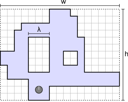
Figure 1: An initial contamination in $\mathcal{C}$. Also depicted are the contamination’s axis aligned bounding box (the rectangle outlined in a dashed way), its width ($w$) and its height ($h$). $\lambda$ is the length of the longest short side among any holes.

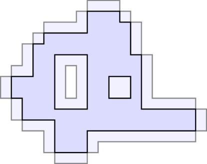
Figure 2: The contamination from Fig. 1. The cells that will become contaminated during a spread are colored lighter.

We want to enable a robot to clean the contamination. Initially, the robot is located in one of the contaminated cells. It can sense the status of the eight cells in its neighborhood; see Fig. 1. In each time unit, the robot can turn, move to one of the four adjacent cells, and decide to clean it. Thus, $d$ measures the robot’s speed against the contamination’s. The robot is a finite automaton. It has no previous knowledge about $C$, and because its memory is of constant size it cannot store a lot of information as it moves around. There is no global control or any other information the robot could make use of.

Whether or not environment $C$ can be cleaned depends on its initial extension and its spreading time relative to the robot’s speed, $d$. Let $h$ and $w$ denote height and width of the bounding box of $C$, respectively. In our model the perimeter of $C$, i.e., the number of edges on its outer boundary, equals $2(h+w)$. Thus, $h+w$ is a reasonable measure for the size of $C$; see Fig. 1.

In Theorem 3 we will establish a geometric lower bound in terms of $h$ and $w$. No robot can clean all environments of height $h$ and width $w$ if its speed $d$ is less than $\sqrt{2}(h+w)-4$ (not even if the robot knows $C$ and has Turing machine power).

Our main contribution is a strategy Smart Edge Peeling (SEP) for which we can prove the following performance guarantee. Let $\lambda$ denote the maximum length of all shorter edges of the rectilinear holes inside $C$; see Fig. 1.

Theorem 1. Given speed $d\geq 3(h+w)+6$, and starting from a contaminated cell, strategy SEP cleans each contamination in $\mathcal{C}$ of height $h$ and width $w$ in at most $(\frac{\lambda}{2}+h+w+5)d$ many steps.

Starting from a contaminated cell, strategy SEP heads for the outer boundary of $C$, without attempting to enlarge any holes. Then it carefully peels the perimeter of $C$, layer by layer, making sure that the set of contaminated cells always stays connected. In order to maintain this invariant the strategy will not clean critical contaminated cells which would destroy connectivity locally. The strategy is precisely defined in Section 4. We have also implemented the strategy. A supplementary video of an execution of the strategy can be found at http://tizian.informatik.uni-bonn.de/Video/smartedgepeeling.mp4 .

Definition 4.

Let $c$ be a contaminated cell. Let $S$ be the set of $c$ and its eight neighbors. Then, $c$ is considered critical if there exist contaminated cells $a,b$ in $S$ with $a\neq b\neq c$, so that all contaminated paths from $a$ to $b$ necessarily lead through $c$.

This concept is taken from pixel-space filling algorithms in computer graphics [15]; see Fig. 3 for an example. Although this constraint causes extra cell visits and possible delay (when cleaning can only be continued once a spread has occurred), our strategy compares favorably with a greedy approach that does not care about connectivity.

Figure 3: In the five examples depicted, the second and the fifth one’s center cell is critical. With respect to the third example, note that we do not consider diagonally adjacent contaminated cells as connected.

In fact, a greedy strategy may completely clean one connected component, being unaware of others. Only after many spreads would it sense that contamination has again reached the robot’s current position. In Theorem 4 we show that this approach can fail if speed $d$ is less than $4(h+w)$, whereas SEP always works if $d\geq 3(h+w)+6$, by Theorem 1. Maintaining connectivity has the additional advantage that the robot knows when the very last cell has been cleaned, so that it could turn to another task.

The rest of this paper is organized as follows. In Section 2 we review related previous work. Strategy SmartEdgePeeling is presented in Section 4. We show how to take advantage of the geometry of the scene (rectangular holes, an outer boundary consisting of four monotonic chains), and design SEP in such a way that these properties are also maintained under spreads and cleaning activities; proving these invariants is a major part of our analysis (Sections 3, 5 and 6). Our main theorem introduced above is then proven in Section 7. Section 8 contains the lower bounds mentioned above, and in Section 9 we state questions for future work.

2 Previous Work

The problem of cleaning expanding domains is located within the field of robot motion planning, which can itself be divided into several sub-fields dependent on the robot’s computational capacities, the a priori knowledge it is given, and the kind of environment it finds itself in.

In offline motion planning, robots are in possession of all relevant information about the problem instance to solve, allowing them to plan their actions in advance, usually employing powerful computational capacities. A good example for this is the family of pursuit-evasion problems (for an overview, see [9]), also known as intruder search, cops and robbers, or lion and man problems [8, 6]. In these problems, the space of the intruder’s possible positions expands and needs to be contained, which can be seen as a rough analogon to the contamination in this article.

In online motion planning scenarios, robots have to collect environment information at run time, for example by local sensor-based perceptions. Our scenario can clearly be located within this field, which however mostly considers static scenarios. A further field somewhat related to our work is online graph exploration (see, for example [9]), as our robots essentially explore dynamic grid graphs. However, in graph exploration problems, in general, less use of geometrical properties is made.

More precisely, our problem can be located in the range of mobile robot covering problems, a form of terrain exploration requiring a robot to visit (”cover”) all places within a given planar terrain. There are two common approaches to covering: Heuristic (for a recent example employing the common A* algorithm see[17]) and analytical, the latter of which aims for guaranteeing complete coverage. Finding optimal-lenght covering paths (also referred to as ”lawn mower problem”) is proven to be NP-Hard [5] which leads to finding approximate solutions. In his 2001 survey [7], Choset classifies analytical coverage approaches with respect to environments tesselated into a grid of square, close-to-robot-sized cells as approximate cellular decompositions; see also [12] for a more recent survey.

To this category our strategy presented in this article can be counted. There exist offline approaches [20] as well as online ones, e.g. [16, 10, 11, 14]. There are also bio-inspired ways of covering making use of stigmergic information like for example exhibited by ants [18].

To the best of our knowledge, we present the first online approach on cleaning expanding grid domains, without adding global information or accumulating knowledge. In addition, in particular when approached in an analytical way, covering is usually adressed with respect to static environments. In contrast, cleaning expanding domains can be seen as a dynamic variant of mobile robot covering.

2.1 Cleaning static and expanding grid domains

Cleaning of grid domains has been investigated first in both a static and a dynamic variant in a family of articles that serve as inspiration for our work [2, 3, 19, 4, 1].

In [19] the special case of static contaminations without holes is addressed. The authors let robots traverse the boundary without central control, peeling off layers by cleaning any non-critical cell they encounter (”edge peeling”).

The authors propose to reuse their strategy with slight variations on the dynamic variant of the problem and present upper and lower bounds on the cleaning time [4, 1, 2]. Extending strategies from the static problem to its dynamic version turns out to be difficult: In particular one cannot neglect holes even if an initial contamination is required to be simply-connected because at any spread parts of the contamination boundary may grow together and create holes out of former boundary parts. Holes however impose serious challenges: Distinction between the outer contamination boundary and hole boundaries with local knowledge (Fig. 4) is non-trivial. It needs to be ensured that robots do not get stuck at holes while the outer contamination boundary expands exceedingly.

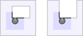
Figure 4: Even though the left robot sees a hole boundary, while the right one sees the outer contamination boundary, both robots have exactly the same perceptions.

In [4], the authors disabled the existence of holes by not allowing them in initial contaminations and requiring the existence of a very helpful elastic membrane. The membrane is an automatically updated global data structure in the grid world that all agents share, see Fig. 6. The robots traverse the membrane instead of the boundary and everything else basically stays the same. On the pro side, it enforces the contamination’s simply-connectedness over time. On the other hand, the contamination’s geometry can get arbitrarily complicated, see Fig. 6. In our work, we allow holes and only require an initial contamination’s geometry to be relatively simple. We guarantee to maintain this simplicity and as a consequence, that no further holes emerge. We do not need a global data structure. The initial geometrical simplicity we require would not have helped in the related work at all, as in the original edge peeling strategies, such a simplicity is not maintained, so new holes can still emerge any time, see Fig. 5.

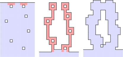
Figure 5: In the left image part, a section of a large, solid rectangular contamination with some minimal holes is illustrated. In the middle, the same section is illustrated after several ”edge peeling” robot traversals. On the right side, we can see the spread outcome of the configuration in the middle.

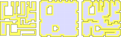
Figure 6: A contamination $C$ (left) and the spread outcomes of $C$ both without membrane (middle) and with membrane (right). Observe that, even though holes emerge, the contamination cannot grow together and stays simply-connected, if the elastic membrane restriction is placed. The membrane does not allow closed contaminated paths around emerging holes.

The authors mention that their strategy could work without a membrane if agents do not get stuck at holes like described above; In this work, we feel it necessary to ensure by only local means that this does never happen.

3 How spreads change contaminations

In order to prove that a contamination does not change the complexity of its geometry during a spread, we firstly need to define some fundamentals. Let $C$ be a contamination and $a,b$ adjacent cells with $a\in C$ and $b\notin C$.

Definition 5.

The edge separating $a$ and $b$ is called a border edge and $C$ is enclosed by a simple grid polygon, $\text{{poly}}(C)$.

Definition 6.

With respect to a clockwise traversal, grid polygons can be seen as an intersection-free closed sequence of atoms, where atoms can be of type border edge, right turn and left turn, see Fig. 7. Note that no turns are located next to each other. The length of any such sequence is the number of border edges it contains.

We use the following naming conventions. $\text{{box}}(C)$ denotes the axis aligned bounding box of $C$, and $0pt{C}$ and $0pt{C}$ the extension from west to east and north to south respectively, see Fig. 1.

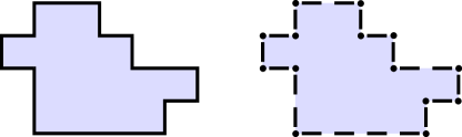
Figure 7: A contamination depicted as enclosed by a grid polygon on the left, and with the grid polygon as a sequence of atoms on the right. On the right, the line segments mark border edges, and the dots mark left and right turns (with respect to a clockwise traversal).

Lemma 1.

Let $C\in\mathcal{C}$. Let $D$ be the outcome of $C$ after a spread. Then, $D\in\mathcal{C}$.

Proof.

Contaminations in $\mathcal{C}$ are enclosed by four monotonic chains. No parts of $\text{{poly}}(C)$ can grow together by a spread, as such configurations would require $\text{{poly}}(C)$ parts growing towards each other and therefore $\text{{poly}}(C)$ to contain an U-turn. Therefore, no new holes can emerge and, as contaminated cells only contaminate their 4Neighborhood, $\text{{poly}}(D)$ consists of four monotonic chains again.

After a spread, the rectangular holes have disappeared or are smaller and still rectangular. Furthermore, as $C$ contained finitely many contaminated cells, $D$ also does. Last, as $C$ was connected, $D$ is also connected. Hence, $D\in\mathcal{C}$. ∎

Definition 7.

The circumference of a contamination $C$, denoted as $\text{{circ}}(C)$, is the length of the shortest closed path of cells $\in C$ that touches every border edge in $\text{{poly}}(C)$.

Note that dependent on $\text{{poly}}(C)$’s shape, some cells may be visited more than once, see Fig. 8. Because of the monotony of the four parts $\text{{poly}}(C)$ consists of, for $C\in\mathcal{C}$, we know:

Lemma 2.

Let $C\in\mathcal{C}$. Then, $\text{{circ}}(c)=20pt{c}+20pt{c}-4$.

Also, obviously, the following holds:

Observation 1.

Let $C$ be a contamination. Let $D$ be its spread outcome. Then $0pt{D}=0pt{C}+2$ and $0pt{D}=0pt{C}+2$.

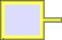
Figure 8: The circumference of a contamination $C$ is the number of steps an agent would have to perform in order to traverse the cells touching $\text{{poly}}(C)$ completely.

From this, we also know $\text{{circ}}(D)=\text{{circ}}(C)+8$. Also note that by spreads, holes are retracted from the outer contamination boundary. In order to formalize this, we need another definition:

Definition 8.

Let the set of all cells touching $\text{{box}}(C)$ be denoted as layer 1. Let the set of 4Neighbors of layer 1 located to the inner side of layer 1 be denoted as layer 2, and so on until every cell in $\text{{box}}(C)$ is assigned to a layer, see Fig. 9.

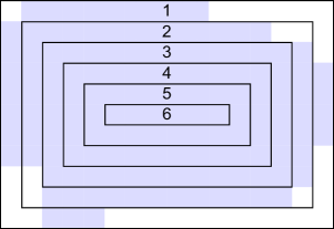
Figure 9: A contamination partitioned into layers with layer numbers depicted.

Lemma 3.

Let $C$ be a contamination and let $C$ contain holes. Let $D$ be the spread outcome of $C$. Then, the outmost hole cell in $D$ is located in a layer $\geq 4$, if such exists.

Proof.

As holes are surrounded by closed paths of contaminated cells, the outmost hole cell in $C$ is in layer $\geq 2$. Layer 2 with respect to $C$ will be layer 3 with respect to $D$. Additionally, all cells in Layer 2 with respect to $C$ have a contaminated 4Neighbor. Thus, all hole cells in layer 2 with respect to $C$ get contaminated during the spread and the outmost remaining hole cell can only be in a layer $\geq 3$ with respect to $C$ or $\geq 4$ with respect to $D$. ∎

4 Cleaning strategy: Smart Edge Peeling

The agent keeps an integer bearing counter for the turns performed, which is initialized with 0. It is increased at $90^{\circ}$ right turns and decreased at $90^{\circ}$ left turns. Note, that the bearing counter can only represent three values, so the limitations of the finite automaton robot model are not violated. Based on its perception of the eight cells around its position, an agent can decide whether or not its position is critical.

We will now define cleaning strategy SEP. In contradistinction to the related work, it will not clean every uncritical boundary cell it encounters to guarantee that the contamination’s geometrical invariants are preserved. A supplementary video of an execution of the strategy can be found at http://tizian.informatik.uni-bonn.de/Video/smartedgepeeling.mp4 .

We assume that in any time step, first a spread takes place if $t=nd$ for $n\in\mathbb{N}$, and second the strategy is started (in the first time step) or resumed (in any further time step). Further, $d>1$, so there cannot be a spread directly before the first time step. The strategy Smart Edge Peeling (SEP) is presented formally in Section 4. The comments are meant to be read together with the below explanations.

Algorithm 1: Strategy Smart Edge Peeling (SEP). Precondition: Agent starts on a contaminated cell. For the sake of readability, it is assumed that the status variables bearingCounter (incremented for each right turn and decremented for each left one) and lastTurnWasRight are maintained automatically. The status of bearingCounter is assumed to be only updated in search mode.

⬇ 1IF spreadDetected OR firstTimeStep: 2 #Initialize / reset status variables 3 lastTurnWasRight = ”false”; #Autom. maintained 4 bearingCounter = 0; #Autom. maintained 5 mode = ”search”; #Can be ”search” or ”boundary” 6 criticalCellPassed = ”true”; 7 8IF locatedOnLastContaminatedCell: 9 cleanCurrentLocation; 10 terminate; 11 12#BLOCK 1. Makes the agent turn right 13#and assesses if it has reached the boundary. 14IF mode == ”search” AND bearingCounter == 0: 15 #Agent moves freely through the contamination. It 16 #may be able to continue its movement or forced 17 #to turn by clean cells around it. 18 IF frontContaminated: 19 #Contaminated cell ahead. No turn needed. 20 ELSE IF rightContaminated: 21 #Clean cell ahead, contaminated one on the right. 22 turnRight; 23 ELSE IF rearContaminated: 24 #Front and right side are clean; turn right two times. 25 #BC reaches 2, which cannot be caused by holes. 26 #So, the agent switches to boundary mode and 27 #resets criticalCellPassed. This flag may be set true 28 #later dependent on the current position’s criticality. 29 turnRight; turnRight; mode = ”boundary”; 30 criticalCellPassed = ”false”; 31 ELSE IF leftContaminated: 32 #Front, right and rear are clean. Turn right three 33 #times and analogously switch to boundary mode. 34 turnRight; turnRight; turnRight; 35 mode = ”boundary”; criticalCellPassed = ”false”; 36ELSE IF mode == ”search” AND bearingCounter == 1: 37 #Agent follows a boundary to its left, but it cannot 38 #know if the boundary belongs to a hole or not. 39 IF leftContaminated: 40 #Turn back to original orientation with BC 0. 41 turnLeft;

⬇ 1#BLOCK 1 continued. Be aware that the next line is an 2#ELSE IF with respect to the IF in line Line 39. 3 ELSE IF frontContaminated: 4 #Left side still clean, contaminated cell ahead. 5 #No turn needed, continue to follow boundary. 6 ELSE IF rightContaminated: 7 #Clean cells ahead and to the left. Agent turns 8 #right again, knowing to have reached the boundary. 9 turnRight; mode = ”boundary”; 10 criticalCellPassed = ”false”; 11 ELSE IF rearContaminated: 12 #Clean cells to the left, front and right. Agent 13 #knows to have reached boundary, turns right twice. 14 turnRight; turnRight; mode = ”boundary”; 15 criticalCellPassed = ”false”; 16ELSE IF mode == ”boundary”: 17 #Agent knows it is at the boundary, follows it using 18 #left hand rule. After right turns, it resets 19 #criticalCellPassed (again: may be set true later). 20 IF leftContaminated: 21 turnLeft; 22 ELSE IF frontContaminated: 23 #Agent just goes ahead, no turn needed 24 ELSE IF rightContaminated: 25 turnRight; criticalCellPassed = ”false”; 26 ELSE IF rearContaminated: 27 turnRight; turnRight; criticalCellPassed = ”false”; 28 29#BLOCK 2: Cleaning and Movement. The agent is 30#allowed to clean if it is in boundary mode, the 31#last turn was a right one and no critical cell 32#was passed after this right turn. 33IF currentPositionCritical: 34 criticalCellPassed = ”true”; 35IF mode == ”boundary”: 36 IF lastTurnWasRight AND NOT criticalCellPassed: 37 cleanCurrentLocation; 38 ELSE IF inTailCell: 39 #Tail cells are always cleaned when in 40 #boundary mode. 41 cleanCurrentLocation; 42moveForward;

Let the agent be deployed somewhere within a contamination $C\in\mathcal{C}$. W.l.o.g. let the agent be starting northwards.

In search mode (from Line 14 on), the agent does not clean any cell, but moves through the contamination searching for the outer boundary. If it encounters any boundary, it turns right (Line 22), increasing its bearing counter. It cannot know if it has found a hole or the outer contamination boundary. As holes are rectangular, they will force the agent to perform a right turn. However, the agent will turn left and move northwards again later on, decreasing the bearing counter to 0 again (Line 41). In this manner, the agent will leave any hole encountered without doing any change to it, (Fig. 10) eventually encountering the outer contamination boundary. Once the bearing counter reaches 2, the agent will know for sure to have reached the outer contamination boundary, and switch to boundary mode (from Line 16 on). Let $\text{{searchtime}}(C)$ be the time the agent has spent until switching to boundary mode.

Lemma 4.

Let $C\in\mathcal{C}$. Then, $\text{{searchtime}}(C)\leq 0pt{C}+0pt{C}-2$.

Proof.

Follows from the fact that the agent has been moving monotonously towards the east and the north (Fig. 10). ∎

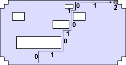
Figure 10: An example search mode trajectory that initially performed by an agent using SEP. As the agent encounters several holes, it’s bearing counter changes between 0 and 1. The first time the agent’s bearing counter reaches 2, the agent switches to boundary mode.

In boundary mode, the agent will follow the boundary using left-hand rule. Before we describe the boundary mode in detail, we need further definitions:

Definition 9.

Let $C\in\mathcal{C}$ and an agent be in boundary mode in $C$. Then we call the following $\text{{circ}}(C)$ steps the agent performs one traversal, if no spread occurs within this time period.

Definition 10.

We call a contaminated cell that touches at least three border edges a tail.

We have to use the time dependence on $C$ for this definition, as we cannot easily put a cell-based traversal definition, for the agent might clean cells and reduce the circumference during a traversal.

Only in boundary mode, cells are cleaned, and critical cells are omitted from cleaning. This immediately leads the following lemma:

Lemma 5.

SEP does not destroy a contamination’s connectivity.

However, cleaning is controlled even more carefully (see Fig. 11): The agent starts a cleaning phase after it performed a right turn on an uncritical cell (Lines 25 and 27), which may even happen together with switching to boundary mode (Lines 29, 34, 9 and 14). Please note, that in these lines, no criticality check is performed. This is done later in the strategy in Line 34. A cleaning phase is stopped when the agent passes left turns (Line 21) or critical cells (Line 34). Additionally, in boundary mode, the agent cleans its current position independently from cleaning phases, if it is located within a tail.

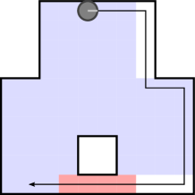
Figure 11: Two agent cleaning phases. The white cells are cleaned as an agent using SEP in boundary mode follows the depicted trajectory. The upper phase is stopped when the agent traverses a left turn, the lower one when a critical cell is traversed. Tail cleaning is not depicted here; we will examine what it is good for later.

The above version of the strategy performs a full reset if a spread is recognized (Line 1). Spreads are recognized if a clean cell located in an agent’s perception range becomes contaminated. In case all cells in an agent’s perception range have been contaminated before a spread, an agent will be unable to recognize a spread – however, in this case the agent moves freely through the contamination in search mode, in which spreads are not relevant for its behavior.

5 How Smart Edge Peeling changes contaminations

We have already seen that $\mathcal{C}$ is closed with respect to spreads. Thus, it remains to examine $\mathcal{C}$ is also closed with respect to SEP cleaning operations. In order to provide an answer to this question, we will now examine when cleaning phases in a contamination $C\in\mathcal{C}$ are started and stopped. Then, we will analyze for one single contaminated cell that is being cleaned by an agent, how $\text{{poly}}(C)$ can possibly be changed.

In the following lemma and proof, we will show that SEP only cleans a cell when it finds itself in one of the eight situations depicted in Fig. 12.

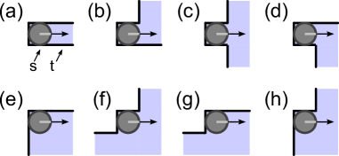
Figure 12: The situations agent cleaning is performed in. A new left turn is only created in situation (e). Situations (a) – (d) are the four possible tail situations, except for rotational symmetry.

Lemma 6.

Let $C\in\mathcal{C}$. Let SEP clean a cell of $C$, yielding contamination $D$. Then, $D\in\mathcal{C}$.

Proof.

Let $C$ consist of more than one cell, otherwise the agent would clean this cell and terminate. Let $s$ be a cell in $C$, let $t$ be a contaminated 4Neighbor of $s$ and let an agent using SEP clean $s$ moving to $t$. W.l.o.g. let $t$ be $s$’s east neighbor. By Section 4 the agent starts cleaning following the boundary right hand rule after it turned right in an uncritical boundary cell before. It stops cleaning when traversing critical cells or turning left. Also, an agent may clean if located in a tail.

Then, $s$’s north neighbor is clean, as otherwise the agent would not be moving east. Further, $s$’s northwest neighbor is clean, otherwise there would be a U-turn in $\text{{poly}}(C)$ and hence $C\notin\mathcal{C}$. As the agent either starts a cleaning phase turning right or continues a cleaning phase or it is located in a tail, $s$’s west neighbor is clean. It remains to examine the possible contamination states of $s$’s southwest, south, southeast end northeast neighbors, which place constraints on each other.

If $s$’s south neighbor is clean, the southwest one also must be clean, otherwise there would again be a U-turn in $\text{{poly}}(C)$ and $C\notin\mathcal{C}$. If the south neighbor is contaminated, the southeast must be contaminated, too, otherwise $s$ would be critical, a contradiction to our assumptions. All the remaining situations are depicted in Fig. 12; they include all in which the agent is located in a tail. In none of the situations, $\text{{poly}}(C)$ is deformed in a way it does not consist of four monotonic chains.

Furthermore, the agent does not destroy a contamination’s connectivity and does not change the shape of holes. All criteria in Definition 2 are preserved, and $\mathcal{C}$ is closed with respect to SEP cleaning operations. ∎

The combination of Lemmata 6 and 1 guarantees that across the whole runtime, we never have to deal with other contaminations than the ones in $\mathcal{C}$. Also, as there can never grow together parts of a contamination enclosing polygon during a spread, no new holes can emerge. We sum up:

Corollary 1.

Let $C\in\mathcal{C}$ be an initial contamination. Let $D$ be a later contamination resulting of spreads and / or SEP cleaning operations on $C$. Then, $D\in\mathcal{C}$ and no new holes did emerge at any spread that may have happened in between.

We examined earlier how spreads carry out influences on width, height and circumference of contaminations. Now, we need to do the same for agents. Note that SEP cleaning operations never increase a contamination’s width and height, as an agent never contaminates cells. Because $\text{{circ}}(C)=20pt{C}+20pt{C}-4$ the circumference is never increased as well. We now examine how they actually get decreased. For this, we need another definition.

Definition 11.

Let us define an ear as a maximal strip of contaminated cells, each adjacent to the same side of $\text{{box}}(C)$.

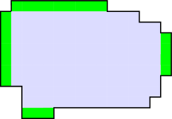
Figure 13: A contamination with ears painted green.

Ears are depicted in Fig. 13. We use the following naming convention. If an ear is adjacent to the north side of $\text{{box}}(C)$, we call it a north ear, and so on. Note that in contaminations in $\mathcal{C}$ there can be no more than one ear per compass direction, because otherwise there would exist an U-turn in $\text{{poly}}(C)$ between ears touching the same $\text{{box}}(C)$ side. Further note, that ears can also overlap, i.e., contaminated cells may belong to more than one ear. For instance, in a contamination consisting of a single cell, the cell marks all four ears.

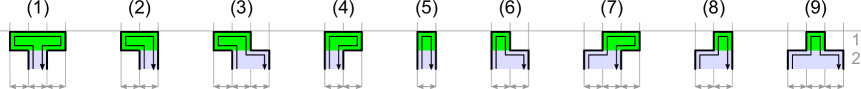
Figure 14: All possible north ear configurations except for stretching. Depicted are the first two layers of the north side of $\text{{box}}(C)$ of a simply-connected contamination $C$. The grey, horizontal line marks the north side of $\text{{box}}(C)$. The equally colored numbers on the right mark the layer numbers. Ear cells are depicted green. Columns surrounded by grey, vertical lines and marked with a $\leftrightarrow$ at the bottom of the figure can have an arbitrary width of $\geq 1$ units. The arrow trajectories mark how the ears are traversed by agents using SEP in boundary mode. Note that while some of the ear configurations might be intuitively considered as impossible in contaminations $\in\mathcal{C}$, actually all of them can occur. Still, the ears whose first or last turn is a left one do impose constraints on the shape of the rest of the contamination. For example, in contaminations $\in\mathcal{C}$, type (1) ears can exist; but not all of the four ears can be of type (1); the leftmost and rightmost cells of the ear would be $C$’s west and east ears.

Lemma 7.

Let $C\in\mathcal{C}$, let the outmost hole cell in $C$ be in a layer $\geq 3$. Let $D$ be the contamination after an agent using SEP performed one traversal on $C$. Then, $0pt{D}\leq 0pt{C}-2$ and $0pt{D}\leq 0pt{D}-2$, respectively, at least four ears have been cleaned.

Proof.

It is easy to assess that $C$ could be cleaned with one agent traversal if $\min(0pt{C},0pt{C})\leq 2$. Hence, let us assume that $\min(0pt{C},0pt{C})>2$.

We will prove that during one traversal, for each compass direction at least one ear is cleaned. W.l.o.g. let us examine the north box side.

Except for stretchings, there are nine possibilities how an ear can look like. See Fig. 14 for all nine possible variants of north ears.

In addition to Fig. 14, in Fig. 15, we prove step by step for two example ear configurations that ears are cleaned in one agent traversal. Observe how critical cells within the ears’ parts protruding to the east and the west lose their criticality during the passing of the ear so they can get cleaned. The cleaning of other ear variants is performed analogously, and every ear is cleaned when completely passed by an agent in boundary mode. Here we make use of the assumption the outmost hole cell in $C$ is located in a layer $\geq 3$. Otherwise, there could exist holes in layer 2 causing critical cells in layer 1 that would not become uncritical in this way and therefore make the cleaning of an ear impossible. If an ear is cleaned, either the contamination’s width or height is reduced by 1, and its circumference is reduced by at least two. Hence, during one traversal, for each compass direction at least one ear is cleaned, proving the lemma. ∎

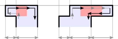
Figure 15: Exact SEP behavior on two example north ears cleaned after one traversal. The left example is a stretched variant of configuration (2) in Fig. 14, the right one of configuration (7). Cells are marked red by their initial state of criticality. In both examples, SEP boundary mode trajectories are included. Every atomic agent movement is marked by an arrow tip on its target. During grey, dotted steps, the agent does not clean. Black, continuous steps mark cleaning of the cell the agent leaves in this step. In both examples, we assume that the agent is not cleaning when entering layer 1. We name the steps alphabetically and reference the line numbers responsible for turning and cleaning in Section 4, where appropriate. Left example. Step A) Agent enters layer 1. B) Moves left (Line 21). C) Turns right twice, cleaning switched on (Lines 27 and 37), rendering target cell uncritical. D) Moving on (Line 23), still cleaning. E) Right turn (Line 25), still cleaning, leaving layer 1. Right example. Ommiting line numbers known from before. A) Enters layer 1. B) Turns right, cleaning switched on. C) Passing critical cell, cleaning switched off again (Line 34). D) Just moving. E) Double right turn, cleaning switched on, rendering target cell uncritical. F) Still cleaning, again rendering target uncritical. G) Left turn (Line 21). Cleaning switched off. However, we are located in a tail, which is cleaned anyway (Line 41). The rest of the configurations can be analyzed analogously.

By this we also know $\text{{circ}}(D)\leq\text{{circ}}(C)-8$.

6 More efficient boundary search

In this section, we will make use of our geometry guarantees and introduce an optimization for boundary searching after a spread in order to resume cleaning earlier after a spread and optimize SEP’s runtime. We call this optimization quick search. As our optimization only affects the SEP’s search mode and not the way of cleaning, the proofs presented so far stay valid.

Lemma 8.

Let $C\in\mathcal{C}$. Let an agent perform SEP, be in boundary mode and let a spread happen. After that, the agent can reach the boundary and switch to boundary mode again within three time steps.

Proof.

Let $D$ be the outcome of $C$ after the spread. By Corollary 1, $D\in\mathcal{C}$. W.l.o.g. let the agent be oriented northwards and traverse $C$’s boundary in boundary mode. There are only few possible situations an agent can find itself in when traversing $C$’s boundary left hand rule, right before a spread occurs. They are depicted in Fig. 16. As $\text{{poly}}(C)$ consists of four monotonic chains, for any of the situations that can occur, green areas are depicted that are guaranteed to be clean in $D$ after the spread occured.

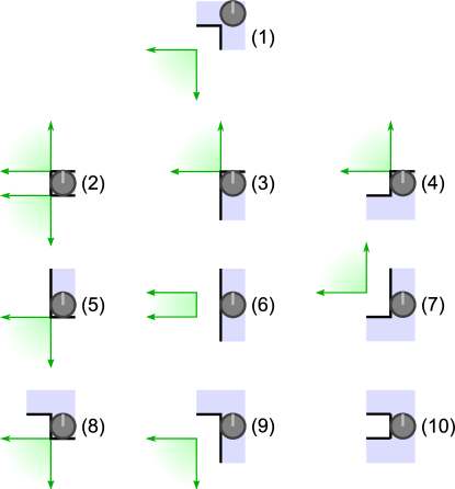
Figure 16: Let $p$ be the agent’s position, and let the agent be in boundary mode oriented northwards. If $p$’s west neighbour is contaminated, situation (1) occurs. If $p$’s west neighbour is clean, we can distinct the 9 cases (2) – (10) dependent on three possible ways $\text{{poly}}(C)$ may turn at each of the ends of the border edge next to the agent. In every of the situations except for (6) and (10), note the green quadrants are guaranteed to be clean even after a spread because of the monotony of the four chains $\text{{poly}}(C)$ consists of. In Situation (6), the green stripe is guaranteed to be clean. Situation (10) cannot occur for contaminations in $\mathcal{C}$.

For any of these possible situations there are cells in the proximity of the agent clean and not part of a hole after the spread. Hence, we propose the following optimized strategy instead of repeatedly performing a full search for the boundary, see Fig. 17: The agent follows a hard-coded path of maximum length three until located at a contaminated cell next to a clean cell. Once located next to one of the depicted cells clean, it turns so that the clean cell is to its left hand side and switches back to boundary mode. If it senses to be located next to a right turn in $\text{{poly}}(C)$, it also sets the lastTurnWasRight variable accordingly. ∎

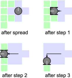
Figure 17: The three hard-coded steps of quick search. After the spread, there is no clean cell within the 4Neighborhood of the agent any more. However, the agent knows one of the green cells must be clean. It then performs the three hard-coded steps depicted until it has found a clean cell, which happens at step 3 at the latest.

Spreads add two to both a contamination’s width and height. If after a spread an agent manages to clean one ear of every compass direction and another fifth ear, it can reduce both width and height of a contamination by two, and one of them by three, shrinking the contamination’s dimensions more than the spread increased them. We now investigate how long this process takes.

Lemma 9.

Let $C\in\mathcal{C}$. Let an agent be in boundary mode on $C$. Let a spread happen, yielding contamination $D$. Given $d\geq 30pt{C}+30pt{C}+6$, before the next spread, SEP cleaning operations yield a contamination $C^{\prime}\in\mathcal{C}$ with $0pt{C^{\prime}}\leq 0pt{C}$, $0pt{C^{\prime}}\leq 0pt{C}$ and $0pt{C^{\prime}}+0pt{C^{\prime}}\leq 0pt{C}+0pt{C}-1$.

Proof.

Let an agent have traversed $C$’s boundary in boundary mode, and let a spread happen. Let $D\in\mathcal{C}$ (Corollary 1) be the outcoming contamination. By Lemma 3 there will be no hole cells in a layer less than 4.

Let us use the following conventions. We denote the most westwards contaminated cell of the north ear as turning point, and analogously for the remaining three compass directions. Each of these turning points is marked by a black dot in Fig. 18, left subfigure of each example. When passing a turning point, an agent turns right, cleaning the ear introduced by the turning point, then leaving it. As the corner cells in $\text{{box}}(D)$ cannot be contaminated after the spread (they cannot have had a contaminated 4Neighbor), we know that $D$’s four ears are of type (9) with respect to Fig. 14. This ear type does not contain any critical cells, and if traversed, is cleaned without the need of a cell to be visited twice.

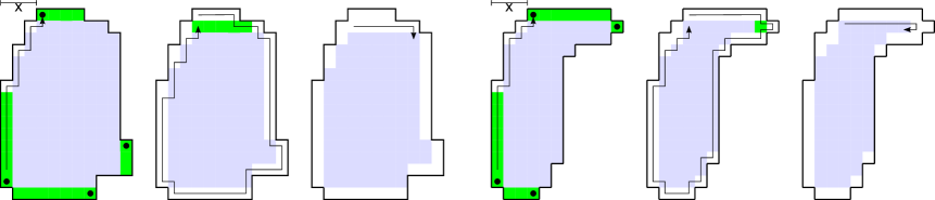
Figure 18: Two examples for agent trajectories when cleaning five ears after quick search. The left three subfigures represent the tree phases described in the proof of Lemma 9. The right three subfigures describe the same three phases, but on another contamination example. We depict the three phases for two contamination examples to illustrate the two cases occuring at the end of the proof of Lemma 9. All ears to be cleaned within the next phase are depicted green. Any phase’s subfigure contains the agent’s trajectory during the phase. In every first phase’s subfigure, turning points are marked by dots.

We split the time until five ears are cleaned into four phases (each starting at the preceding phase’s end or after the spread, respectively):

• Phase 1, until the agent reaches the first turning point,

• phase 2, until the first four ears of type (9) are cleaned,

• phase 3, until the last ear is cleaned.

Phase 1. Getting back to boundary mode takes the agent three time steps (Lemma 8). In the worst case, the agent just missed a turning point. W.l.o.g. let it miss the west one, so the first turning point to pass is the one of the north ear. Between two turning points, an agent moves in a monotonous trajectory (Fig. 18, left subfigure of each example). In the vertical, the agent has to cover a distance of $0pt{D}-3$ in the worst case (assuming the north ear started most to the west and its turning point was only missed most closely). In the horizontal, the agent has to cover $x$ cells to reach the westmost cell of the north ear, where $x\geq 1$ (the corner cells in $\text{{box}}(D)$ cannot be contaminated for they cannot have had a contaminated adjacent cell). Overall, phase 1 needs $0pt{D}+x$ time steps.

Phase 2. As a spread just happened, the outmost hole cell in $D$ can be only in a layer $\geq 4$ Lemma 3. By Lemma 7, within one traversal the agent is able to clean $D$’s north, east, south and west ear. One traversal takes $20pt{D}+20pt{D}-4$ time steps (Lemma 2, Definition 9) and is depicted in Fig. 18, middle subfigure of each example. As by its cleaning operations, the contamination lost one unit of height in the meantime, the agent needs even one step fewer than a traversal: $20pt{D}+20pt{D}-5$ time steps. After that, the agent is located within a new north ear in a horizontal distance of $x$ to the north side of the original $\text{{box}}(D)$.

Phase 3. With respect to the original $\text{{box}}(D)$ the Agent is located in layer 2 and hole cells can only exist in layers $\geq 4$, so holes cannot cause critical cells in the north ear to clean. Additionally, by the traversal performed in phase two, all cells adjacent to the east side of $\text{{box}}(D)$ are clean. Hence, the agent needs at most $0pt{D}-x-2$ cells to reach the east end of the north ear. There are two cases:

• The ear does not contain any cells protruding to the east, namely has been of types (2), (3), (5), (6), (8) or (9) with respect to Fig. 14. In this case, the agent cleans the ear’s last cell and heads south.

• The ear does contain cells protruding to the east, it has been of types (1), (4), or (7). In this case, the agent finds itself in the eastmost cell of the north ear, which however is also an east ear. It cleans the cell, as it is also a tail, and heads west again. In this case, contrary to our expectations, the agent cleaned an east ear, not a north one.

Both cases consume one further time step. Phase 3 needs $0pt{D}-x-1$ time steps. A contamination example yielding the former case is depicted in the three left subfigures of Fig. 18, one yielding the latter case in the three right subfigures. Phase 3 is depicted in the right subfigure of each example.

All three phases together need $30pt{D}+30pt{D}-6$ time steps, which, by Obs. 1, equals $30pt{C}+30pt{C}+6$ time steps. Let the contamination after this period of time be $C^{\prime}$. By 1, $C^{\prime}\in\mathcal{C}$. Furthermore, for every compass direction, one ear has been cleaned, and one additional ear has been cleaned, so $0pt{C^{\prime}}\leq 0pt{C}$ and $0pt{C^{\prime}}\leq 0pt{C}$. By the fifth ear cleaned, additionally $0pt{C^{\prime}}+0pt{C^{\prime}}\leq 0pt{C}+0pt{C}-1$. ∎

7 Correctness and run time

We now prove the theorem already stated in the introduction. Let $\lambda$ denote the maximum length of all shorter edges of the rectilinear holes inside a contamination $C\in\mathcal{C}$ ($\lambda=0$ if there do not exist such). First, let us recall the theorem.

Theorem 1.

Given speed $d\geq 3(h+w)+6$, and starting from a contaminated cell, strategy SEP cleans each contamination in $\mathcal{C}$ of height $h$ and width $w$ in at most $(\frac{\lambda}{2}+h+w+5)d$ many steps.

Proof.

We use the following naming convention: $C_{i}$ is the contamination that evolved out of $C$ by agent cleaning operations and spreads until the end of time step $i$. As the initial contamination $C$ is in $\mathcal{C}$, all $C_{i}$ are as well (Corollary 1), so all the below referenced lemmata are applicable.

During the first spread phase, $d$ is large enough to allow the agent to find the boundary (Lemma 4) and perform at least one full traversal (Definition 9). In the worst case, the agent is unable to reduce the contamination’s dimensions due to badly placed holes. In this case, the agent has to wait for the first spread, yielding contamination $C_{d}$ with height $h+2$ and width $w+2$ (Obs. 1). By $d\geq 3(h+w)+6$ and Lemma 9 we know that after the spread, the agent decreases the contamination’s width and height more than the spread did increase them. Hence, $0pt{C_{2d-1}}+0pt{C_{2d-1}}\leq 0pt{C_{d-1}}+0pt{C_{d-1}}-1$.

This reasoning is applicable from any further spreadphase’s end to the next: $0pt{C_{(i+1)d-1}}+0pt{C_{(i+1)d-1}}\leq 0pt{C_{id-1}}+0pt{C_{id-1}}-1$. From the end of any spreadphase to the end of the next. Overall, the agent needs at most $w+h+4+1$ spread phases to completely clean the contamination.

Greater $d$ allow for more width and height reduction per spread phase, leading to fewer needed spread phases. Holes however may impair the agent’s usage of such large $d$ and force it to wait for further spreads. After $\frac{\lambda}{2}$ spread phases, all holes are fully contaminated, leading to $\frac{\lambda}{2}+h+w+5$ necessary spread phases overall. ∎

Without holes or holes located in deeper layers, the agent can make use of even larger $d$, leading to an arbitrarily large reduction of the contamination’s width and height per spread phase and therefore fewer necessary spread phases. Hence we can conclude that while our strategy was designed for purely local handling of more complex scenarios, it also competes well on simply-connected and static scenarios.

8 Lower bounds

Our lower bounds are based on the following isoperimetric inequality that can be found, e.g., in Altshuler et al. ([4, Theorem 8]).

Theorem 2.

Let $C$ be a contamination of $c$ cells. Then at least $2\sqrt{2c-1}$ new cells will be contaminated in the next spread.

This bound is attained for the diamond shapes (or $L_{1}$-circles) that result from the spreading of a single contaminated cell; see Fig. 19. Here all but four newly contaminated cells are infected by two neighbors, minimizing the contamination increase.

Theorem 3.

An $h\times h$ square $C$ cannot be cleaned at speed $d<\sqrt{2}\ 2h-4$.

Proof.

Before the first spread occurs, at least $c=h^{2}-d$ cells of square $C$ are still contaminated. By Theorem 2, at least $2\sqrt{2(h^{2}-d)-1}$ cells will become newly contaminated. If this number is $>d$, an even larger number $c^{\prime}>c$ of cells will remain contaminated before the second spread occurs, and so on, proving that cleaning $C$ is impossible. Because of

$$2\sqrt{2(h^{2}-d)-1}>d\ \Longleftrightarrow\ 8h^{2}+12>(d+4)^{2}$$

the claim follows from $d+4<\sqrt{2}\ 2h$. ∎

Since the lower bound of Theorem 3 is not based on the robot’s incomplete knowledge it applies to optimum offline solutions, too. The next result, in contradistinction, holds only for the online strategies we are considering.

Theorem 4.

Let $G$ be a strategy that always cleans the current cell if contaminated, moves to a contaminated cell in its 8-neighborhood, if there is one, and rests, otherwise. Then $G$ cannot clean all strips of length $w$ at speed $d<4(w+h)-16$.

Proof.

Consider a single row of cells, as shown in Fig. 20. The robot starts from an interior cell, cleans it and moves straight to the left or to the right until the end of the strip is reached. Let us assume it moves to the right. At this point we define the initial contamination such that only one of $w=l+2$ cells is situated to the left of the robot’s start position, which remains contaminated as the robot cleans the other $l+1$ cells. While the robot rests at the rightmost cell, contamination spreads from the leftmost cell as shown in Fig. 20. After $l$ spreads, a diamond shape of $2l^{2}+2l+1$ cells is contaminated, among them the cell to the left of the robot. Before the $(l+1)$-st spread occurs, $c=2l^{2}+2l+1-d$ cells are left contaminated. By Theorem 2, at least $2\sqrt{2c-1}$ cells will become newly infected. We have

$$2\sqrt{2(2l^{2}+2l-d+1)-1} >d$$

$$\Longleftrightarrow 16l^{2}+16l+20 >(d+4)^{2}$$

which holds true because of $d<4l-4$. Hence, the increase in contamination will always exceed the maximum number $d$ of cells the robot can clean between spreads. ∎

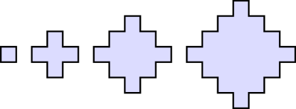
Figure 19: From the left to the right: A minimal contamination after 0, 1, 2 and 3 spreads.

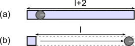
Figure 20: (a) A straight contaminated line of cells of length $l+2$ with the greedy agent’s starting position. (b) The greedy agent destroying it’s connectivity.

The same result can be shown if we allow a greedy strategy $G$ to perform a kind of search for contaminated cells once no contaminated cell is left in its current neighborhood. This is because the robot is a finite state machine, so that only a cyclic search path pattern of constant diameter could result from this capability. If the start and end positions of the pattern are not equal, the agent translates through the space in a constant direction, never visiting cells on the opposite direction.

9 Conclusions and further research

In this article, we presented a cleaning strategy SEP enabling a single finite automaton robot to clean expanding contaminations by only local means. SEP maintains geometric invariants and additionally ensures that the contaminated cells stay connected. Furthermore, we proved that greedy strategies violating the latter principle need greater spreading times $d$ than SEP in general. We considered contaminations $\in\mathcal{C}$, i.e., with certain limitations on their geometric complexity. Besides improving lower bounds, our results suggest two main directions to obtain qualitative enhancements on the task of cleaning expanding contaminations.

One way of generalizing our work is to consider contaminations with arbitrarily complex shapes (Fig. 21), which inadvertently raise further challenges. For example, new holes can emerge in spreads and be of likewise geometrical complexity, or existing holes may split. Some of the lemmata we in this article can already be generalized to higher geometrical complexities. However, to be able to generalize the entire work, more geometrical analysis is necessary.

Figure 21: A contamination with high geometrical complexity. In a spread, new holes would emerge and existing holes would be split.

A further interesting question is how to use a swarm of $k$ agents cleaning expanding contaminations in parallel in order to increase cleaning speed and exhibit fault tolerance known from biological systems.

We are confident that both ways of generalization lead to qualitatively new results. They are subject to our current research.

References

- [1] Y. Altshuler and A. M. Bruckstein. Static and expanding grid coverage with ant robots: Complexity results. Theoretical Computer Science, 412(35):4661–4674, 2011.
- [2] Y. Altshuler, A. M. Bruckstein, and I. A. Wagner. Swarm robotics for a dynamic cleaning problem. In Swarm Intelligence Symposium, 2005. SIS 2005. Proceedings 2005 IEEE, pages 209–216. IEEE, 2005.
- [3] Y. Altshuler, I. A. Wagner, and A. M. Bruckstein. Shape factors effect on a dynamic cleaners swarm. In ICINCO (MARS Workshop), 2006.
- [4] Y. Altshuler, V. Yanovski, I.A. Wagner, and A.M. Bruckstein. Multi-agent cooperative cleaning of expanding domains. The International Journal of Robotics Research, 30(8):1037–1071, 2011.
- [5] E. M. Arkin, S. P. Fekete, and J. S. B. Mitchell. Approximation algorithms for lawn mowing and milling. Computational Geometry, 17(1):25–50, 2000.
- [6] F. Berger, A. Gilbers, A. Grüne, and R. Klein. How many lions are needed to clear a grid? Algorithms, 2(3):1069–1086, 2009.
- [7] H. Choset. Coverage for robotics–a survey of recent results. Annals of mathematics and artificial intelligence, 31(1-4):113–126, 2001.
- [8] A. Dumitrescu, I. Suzuki, and P. Zylinski. Offline variants of the lion and man problem. In Proceedings of the twenty-third annual symposium on Computational geometry, pages 102–111. ACM, 2007.
- [9] F. Fomin and D. Thilikos. An annotated bibliography on guaranteed graph searching. Theoretical Computer Science, 399(3):236–245, 2008.
- [10] Y. Gabriely and E. Rimon. Spiral-stc: An on-line coverage algorithm of grid environments by a mobile robot. In Proceedings. ICRA’02. IEEE International Conference on Robotics and Automation, volume 1, pages 954–960. IEEE, 2002.
- [11] Y. Gabriely and E. Rimon. Competitive on-line coverage of grid environments by a mobile robot. Computational Geometry, 24(3):197–224, 2003.
- [12] E. Galceran and M. Carreras. A survey on coverage path planning for robotics. Robotics and Autonomous Systems, 61(12):1258–1276, 2013.
- [13] S. Garnier, J. Gautrais, and G. Theraulaz. The biological principles of swarm intelligence. Swarm Intelligence, 1(1):3–31, 2007.
- [14] E. Gonzalez, O. Alvarez, Y. Diaz, C. Parra, and C. Bustacara. Bsa: a complete coverage algorithm. In Robotics and Automation, 2005. ICRA 2005., pages 2040–2044. IEEE, 2005.
- [15] D. Henrich. Space-efficient region filling in raster graphics. The Visual Computer, 10(4):205–215, 1994.
- [16] C. Icking, T. Kamphans, R. Klein, and E. Langetepe. Exploring simple grid polygons. Computing and Combinatorics, pages 524–533, 2005.
- [17] A. Ntawumenyikizaba, Hoang Huu Viet, and TaeChoong Chung. An online complete coverage algorithm for cleaning robots based on boustrophedon motions and a* search. In 2012 8th International Conference on Information Science and Digital Content Technology (ICIDT), volume 2, pages 401–405, 2012.
- [18] I. A. Wagner, M. Lindenbaum, and A. Bruckstein. Distributed covering by ant-robots using evaporating traces. Robotics and Automation, IEEE Transactions on, 15(5):918–933, 1999.
- [19] I.A. Wagner, Y. Altshuler, V. Yanovski, and A.M. Bruckstein. Cooperative cleaners: A study in ant robotics. The International Journal of Robotics Research, 27(1):127–151, 2008.
- [20] A. Zelinsky, R. Jarvis, J. Byrne, and S. Yuta. Planning paths of complete coverage of an unstructured environment by a mobile robot. In Proceedings of international conference on advanced robotics, volume 13, pages 533–538, 1993.