Non Parametric Estimates of Option Prices Using Superhedging

Abstract.

We propose a new non parametric technique to estimate the CALL function based on the superhedging principle. Our approach does not require absence of arbitrage and easily accommodates bid/ask spreads and other market imperfections. We prove some optimal statistical properties of our estimates. As an application we first test the methodology on a simulated sample of option prices and then on the S&P 500 index options.

1. Introduction

A classical exercise in the econometric analysis of financial markets is to estimate option prices and the risk neutral probability (or its density) which is implicit in them, as suggested by the famous works of Breeden and Litzenberger [5] and of Banz and Miller [3]. Of special importance in this exercise is the use of non parametric techniques which have become popular in the last decades. Regardless of the econometric approach taken, a first step of crucial importance is purging the data from observations violating some no-arbitrage condition and thus conflicting with the conclusion that prices are the expected value of the asset discounted payoff computed with respect to the risk neutral probability, as assumed by Breeden and Litzenberger.

Recalcitrant observations may however originate from different sources other than just pure mispricing. There are first some microstructural issues, such as the bid/ask spread or other transaction costs, which are not considered in the risk neutral approach. The common practice is to assume that these components are uncorrelated with the fundamental value of the assets and may therefore be disposed of with simple transformations, such as computing mid prices. Nevertheless, a more accurate investigation reveals that market makers often adjust the spread in response to pressure originating either from demand or supply, a fact that contributes to make the spread asymmetric and to induce a possibly significant correlation with the fundamental price. A second factor influencing market data is the existence of restrictions to trading, these too often overlooked in asset pricing models which typically assume the space of marketed claims to be linear. The extreme versions of these restrictions take the form of short selling prohibitions but even with less drastic market rules, the possibility of shorting assets is clearly delicate and subject to constraints such as the provision of appropriate margins the effect of which receives in general little attention – if any – in theoretical and applied work on options. In fact, violations of the lower bound for CALL options, a mispricing that may be exploited by shorting the underlying, are often more frequent than others associated with strategies involving positions which are easier to take. Some additional noise arises with strategies which prescribe to invest simultaneously on different markets, a characteristic which results not only in relevant fixed costs but also in the lack of trade synchronism thus inducing additional risks in the execution of arbitrage strategies. A further issue arises eventually in connection with the riskless asset appearing in virtually all financial models and definitely in all empirical exercises. The assumption of a riskless asset and its explicit identification in applied work appears more and more counter factual as the interbank market turmoil in the years 2007-08 and the sovereign debt crisis following it have clearly demonstrated. Not only during periods of crisis it cannot be assumed that bonds are riskless but it is also hard to assert that the implicit risks are uncorrelated with the equity market.

Of course, the relevance of the preceding remarks would be much less disturbing if one could restrict attention to just the options market and consider only trading strategies which involve long positions. Unfortunately in this restricted perspective the fundamental premise of the Breeden Litzenberger exercise, i.e. that option prices are set on the basis of a risk neutral probability, cannot be assumed. Nevertheless, even if real option prices may fail to possess some fundamental properties, the superhedging price, conveniently computed will possibly satisfy them under mild conditions which involve only very simple and realistic trading strategies. The first step of our econometric approach consists of replacing original option prices with superhedging prices.

As a matter of fact this idea is not new. Aït-Sahalia and Duarte [1] have inaugurated a two stage approach to non parametric estimation of option prices under shape restrictions which, in the first stage, prescribes to project market prices following a methodology adapted from Dykstra [8]. This procedure enforces the shape restrictions required. In the second stage, the prices so transformed are smoothed out using a local polynomial technique, a methodology which generalizes suitably the kernel by replacing constant functions with polynomials of arbitrary but preassigned degree. It turns out, as will be shown in the body of the paper, that the projection technique suggested by Dykstra produces just the options superhedging price, $q^{0}(k)$ – with $k$ the strike price. The need for additional smoothing arises because the CALL function obtained, $k\to q^{0}(k)$ is piecewise linear and therefore not informative enough for many a purpose, including the project to extract a probability density.

In a recent paper, [6], we have obtained a result which is particularly useful for the present purposes and that lays the ground for our non parametric procedure. It states, roughly put, that it is possible to compute explicitly the superhedging price $q^{G}(t)$ for a large class $G$ of derivatives written on the same underlying and with payoff depending in a convex and decreasing way on a positive parameter, $t$. Not only, but for each such family $G$ of derivatives it is possible to extract from the prices $q^{G}(t)$ a probability measure, $\nu^{G}$, implicit in them in much the same way as suggested by Breeden and Litzenberger. A special case is of course the family $G^{0}$ corresponding to plain options but in general the choice of the family $G$ is open. Our suggestion is to consider new derivatives with a payoff which, while being perfectly smooth, approximates the option payoff uniformly. Moreover, the degree of approximation should be made sample dependent so to obtain good asymptotic properties. As long as these properties are guaranteed, any candidate $G$ is suitable, more or less as the functional form of kernels is relatively unimportant in comparison with the choice of the bandwidth. We have found it easy to work with splines but it should made clear from the outset that our use of splines has nothing to do with the econometric approaches based on this class of functions, such as those reviewed by Eubank [9] and successfully applied to options by Fengler and Hin [11]. Our problem in fact is not that of smoothing the option prices (or their implied volatility surface) but rather the option payoff. Splines simply turn out to be a conveniently tractable tool from a computational point of view; in addition, the smoothness/goodness of fit trade off may be tuned conveniently via a parameter acting as the bandwidth in kernel estimation. Other smoothing techniques may be employed, e.g. those based on some known probability density function. As a term of comparison, we shall briefly discuss the result obtained by smoothing options via the normal density rather than splines.

The econometric analysis of option prices has grown over the years to become almost a field of its own and has been masterly reviewed by Garcia, Ghysels and Renault in [13]. The interested reader may find in their work an exhaustive list of references that we shall not try to improve upon here, for reasons of brevity. The non parametric approach has itself produced quite a number of important contributions that are worth discussing briefly with no pretension of completeness. A forerunner of this stream of studies is the paper by Jackwerth and Rubinstein [17] in which the parameters of a binomial tree are set so as to minimize the distance between binomial and actual option prices given a penalty for deviations from an initial a priori distribution. The assumption of absence of arbitrage opportunities is absolutely crucial here and is embodied in the tree parameters. Estimating the option price produces simultaneously an estimate of the risk neutral measure. Aït-Sahalia and Lo [2] estimate the CALL function using the Nadaraya-Watson kernel and recover the risk-neutral density by computing the second derivative. This methodology has optimal asymptotic properties but relatively poor performance in small samples, a fact common to many non parametric methods and of special concern for options market. The curse of dimensionality problem, see [25, p. 675], requires to limit as much as possible the number of state variables. For example, the risk neutral density estimated in [2] via kernel smoothing is surely convergent to the true density but may fail even to be non negative in small samples [2, footnote 11, p. 508]. To circumvent this problem the authors propose a semi nonparametric approach in which the price is computed according to the Black and Scholes formula in which the volatility function is estimated non parametrically. This choice has the clear advantage of guaranteeing the correct shape of the CALL function. Shape restrictions are easily accommodated in parametric modeling but are much more troublesome in the non parametric approach. Papers implementing the nonparametric methodology with shape restrictions are less numerous and more recent. Further to Aït-Sahalia and Duarte [1], another example of non parametric techniques incorporating shape restrictions is the paper by Yatchew and Härdle [26] who follow a least squares approach in Sobolev spaces. There exist eventually several papers who adopt spline techniques to estimate option prices and one should mention Fengler [10], Fengler and Hin [11] and Yin, Wang and Qi [27].

We think that if our approach has any merit compared to the above references, then this lies in its clear financial interpretation. In fact we obtain the smoothness of the CALL function by pricing an appropriate derivative rather than performing some local averaging or implementing some other statistical technique. Moreover, our method allows to take selection effects into full account, a fact not always clearly considered. Eventually the estimates produced are extremely tractable computationally speaking and have desirable convergence properties.

The paper is structured as follows. In section 2 we introduce the fundamental results obtained in [6] and needed in our exercise, together with the necessary notation. In section 3 we illustrate all details of our spline based technique and prove some of its properties. We also comment on the possibility of using given density functions. In section 4 we perform some numerical experiments on option prices generated by an a priori model. In particular we construct non parametric interval estimates in the presence of a realistic structure of noise. Eventually in section 5 we apply the proposed methodology to a sample of S&P option prices. All proofs are in the Appendix.

Let us mention in closing that, although as dictated by the literature on this topic we start assuming the existence of a given probability space, $(\Omega,\mathscr{F},P)$, the results developed in [6] do not require this classical premise.

2. Option Pricing

Most of this section is adapted from [6]. Let the random variable $X$ represent hereafter the payoff of a given underlying and $K(X)$ the set of strike prices (including $k=0$) of all CALL options written on it. We assume $P(X>0)=1$ and $P(X<k)>0$ for all $k\in K(X)\setminus\{0\}$. The portfolio consisting of one option with strike price $k\in K(X)$ and its price will be indicated by the symbols $\theta(k)$ and $q(k)$ respectively. Moreover, its payoff will be denoted with the symbol $g^{0}_{k}(X)=(X-k)^{+}$. As we only consider long positions, $q(k)$ will actually be the ask price and we shall assume that it is positive. The set $\Theta$ of admissible trading strategies is a convex set of portfolios formed by taking long positions in the set of traded options. The price and the payoff of $\theta=\sum_{n=1}^{N}\alpha_{n}\theta(k_{n})\in\Theta$ – so that $\alpha_{1},\ldots,\alpha_{N}\geq 0$ and $k_{1},\ldots,k_{N}\in K(X)$ – are denoted respectively by

(1) $$q(\theta)=\sum_{n=1}^{N}\alpha_{n}q(k_{n})\qquad\text{and}\qquad g^{0}_{\theta}(X)=\sum_{n=1}^{N}\alpha_{n}g^{0}_{k_{n}}(X)$$

The price function $q$ does not include possible fixed trading costs. The apparent linear structure implicit in (1), notwithstanding the existence of bid/ask spreads (which many authors associate with subadditivity of prices, see [6]), is due to the restriction included in $\Theta$ that only long positions may be assumed and the traditional anonymity of option trading. OTC trading of options follows, as is well known, different pricing schemes, often ad hoc, and our theory does not apply to these transactions.

We define the superhedging price of an arbitrary random quantity $h:\Omega\to\mathbb{R}$ as

(2) $$\pi(h)=\inf\Big{\{}\lambda q(\theta):P\big{(}\lambda g^{0}_{\theta}(X)/(X\wedge 1)\geq h\big{)}=1,\lambda>0,\theta\in\Theta\Big{\}}$$

Write $q^{0}(k)=\pi\big{(}g_{k}^{0}(X)/(X\wedge 1)\big{)}$. We say that an option with strike price $k$ is priced efficiently if $q(k)=q^{0}(k)$ and denote by $K^{0}(X)=\{j_{0},\ldots,j_{I}\}$ the set of strike prices for which we have an efficient price. It is easily shown that necessarily $j_{0}=0$. Remark that the notion of efficiency adopted here is particularly poor as it only involves investments with long positions in CALL options and the underlying. Neither PUT options, Futures nor bonds are contemplated. This is desirable since the larger the set of derivatives involved the more likely is it that efficiency may fail, as in the case of the PUT/CALL parity.

We make the following

Assumption 1.

Let $\bar{X}=\mathrm{ess}\sup X$ and assume that

(3) $$\bar{X}>j_{I}\quad\text{and}\quad\mathrm{ess}\sup(X\wedge z)=\bar{X}\wedge z\quad\text{ for each }z\in\mathbb{R}$$

Denote by $\Gamma$ the set of convex functions $g:\mathbb{R}_{+}\to\mathbb{R}_{+}$ with $g(0)=0$ and $\lim_{n\to\infty}g(n)/n<\infty$. Clearly, the function $g^{0}_{t}$ introduced above and corresponding to the option payoff is an element of $\Gamma$ for all $t\geq 0$: write $G^{0}=\{g^{0}_{t}:t\geq 0\}$. Of course, it is possible to write other derivatives on $X$ possessing some of the properties of options. In the Appendix we prove the following:

Theorem 1.

For each $f\in\Gamma$ there exists $\theta(f)\in\Theta$ such that $\pi\big{(}f(X)/(X\wedge 1)\big{)}=q\big{(}\theta(f)\big{)}$ and

(4) $$q\big{(}\theta(f)\big{)}=[q(j_{0}),\ldots,q(j_{I})]\left[\begin{tabular}[]{cccc}$(j_{1}-j_{0})$&$0$&$\ldots$&$0$\\ $(j_{2}-j_{0})$&$(j_{2}-j_{1})$&$\ldots$&$0$\\ $\vdots$&$\vdots$&$\ddots$&$\vdots$\\ $d_{0}(\bar{X})$&$d_{1}(\bar{X})$&$\ldots$&$d_{I}(\bar{X})$\end{tabular}\right]^{-1}\left[\begin{tabular}[]{c}$f(j_{1})$\\ $\vdots$\\ $f(j_{I})$\\ $\hat{f}(\bar{X})$\end{tabular}\right]$$

where $d_{i}(\bar{X})=(\bar{X}-j_{i})$ and $\hat{f}(\bar{X})=f(\bar{X})$ if $\bar{X}<\infty$ or else $d_{i}(\bar{X})=1$ and $\hat{f}(\bar{X})=\lim_{n}f(n)/n$. In particular, we can write

(5) $$q\big{(}\theta(f)\big{)}=\sum_{i=0}^{I}w_{i}q(j_{i})=\sum_{i=1}^{I}b_{i}f(j_{i})+b_{I+1}\hat{f}(\bar{X})$$

Let $D_{i}(h)=\frac{h(j_{i+1})-h(j_{i})}{j_{i+1}-j_{i}}$ when $i=0,\ldots,I-1$ and $D_{-1}(h)=D_{I}(h)=0$. Then, if $\bar{X}=\infty$ we have

(6a) $$w_{I}=\hat{f}(\bar{X})-D_{I-1}(f),\quad b_{I+1}=q(j_{I})$$

(6b) $$w_{i}=D_{i}(f)-D_{i-1}(f)\quad\text{and}\quad b_{i+1}=D_{i+1}(q)-D_{i}(q)\qquad i=0,\ldots,I-1$$

The next result is just a restatement of [6, Theorem 7].

Theorem 2.

Let $G=\{g_{t}:t\in\mathbb{R}_{+}\}$ be a collection of functions $g_{t}\in\Gamma$ such that

(7) $$\alpha g_{s}+(1-\alpha)g_{u}\geq g_{t}\qquad\text{whenever}\quad\alpha\in[0,1],\ s,t,u\in\mathbb{R}_{+}\quad\text{and}\quad\alpha s+(1-\alpha)u\leq t$$

Write $q^{G}(t)=\pi\big{(}g_{t}(X)/(X\wedge 1)\big{)}$. There exists $\beta^{G}\geq 0$ and $\nu^{G}\in ca\big{(}\mathscr{B}(\mathbb{R}_{+})\big{)}$ such that

(8) $$q^{G}(t)=\beta^{G}+\int_{t}^{\infty}\nu^{G}(x>z)dz\qquad\text{for all }t\geq 0$$

Observe that, by standard rules,

(9) $$\int_{t}^{\infty}\nu^{G}(x>z)dz=\int(x-t)^{+}d\nu^{G}(x)$$

Thus (8), represents the price of the $G$ derivatives as the sum of a bubble part and of their fundamental value. This view is substantiated by the observation that necessarily

(10) $$\beta^{G}=\lim_{t\to\infty}q^{G}(t)$$

so that, upon choosing $G=G^{0}$, the term $\beta^{0}$ represents the option price as the strike approaches infinity and contributes to explaining the overpricing of deeply out of the money CALL’s often documented empirically in some form of the smile effect.

As remarked in [6], Breeden and Litzenberger formula applies, giving:

(11) $$\nu^{G}(x>t)=-\left.\dfrac{dq^{G}(k)}{dk}\right|_{k=t}\qquad\text{for all }t\geq 0$$

while in the model of Black and Scholes one has, as is well known,

(12) $$\nu^{BS}(x>k)=e^{-rT}\Phi(d_{2})\quad\text{with}\quad d_{2}=\frac{\ln(S_{0}/k)+(r-\frac{1}{2}\sigma^{2})T}{\sigma\sqrt{T}}$$

so that $\big{\|}\nu^{BS}\big{\|}=\exp(-rT)$. Observe that in our setting, we do not have an a priori restriction on the norm of $\nu^{G}$ because our market does not include any riskless bond.

3. Estimating the CALL function

For what concerns the choice of $G$, it is natural to start considering the family $G^{0}$. By construction $q^{0}(k)$ represents the efficient price of the corresponding option and so it coincides with $q(k)$ if and only if $k\in K^{0}(X)$. More generally one sees that the function $q^{0}$ is the highest among the positive, convex and decreasing curves passing through the knots $\{(j,q(j)):j\in K^{0}(X)\}$. Aït-Sahalia and Duarte [1] obtain the same values in the first step of their approach. Since we have to make a choice for definiteness let’s assume henceforth

Assumption 2.

$\bar{X}=\infty$.

Replace $g$ with $g^{0}_{k}$ in Theorem 1. Then, according to (6), the cheapest way to superhedge the corresponding option is to invest

$$w^{0}_{i}(k)=\frac{j_{i+1}-k}{j_{i+1}-j_{i}}\quad\text{and}\quad w^{0}_{i+1}(k)=1-w^{0}_{i}(k)$$

in the options with strike prices $j_{i}$ and $j_{i+1}$ respectively, where $j_{i+1}\geq k>j_{i}$, and nothing in all other options; or else, if $k>j_{I}$, to buy one unit of the option with strike price $j_{I}$. The corresponding superhedging price would be

(13) $$q^{0}(k)=\left\{\begin{tabular}[]{lll}$\frac{j_{i+1}-k}{j_{i+1}-j_{i}}q(j_{i})+\frac{k-j_{i}}{j_{i+1}-j_{i}}q(j_{i+1})$&if&$j_{i}<k\leq j_{i+1}$\\ $q(j_{I})$&if&$j_{I}<k$\end{tabular}\right.$$

Observe that the CALL function $k\to q^{0}(k)$ satisfies: (i) $q^{0}(j_{i})=q(j_{i})$ for $i=0,\ldots,I$ and (ii) it is a straight line on each interval $[j_{i},j_{i+1}]$ for $i=0,\ldots,I-1$ and on $[j_{I},\infty)$. Then it coincides with the projection obtained by following Dykstra’s method, see [8, sec. 4.1].

From (13) we deduce easily that

(14) $$\nu^{0}(x>k)=\left\{\begin{tabular}[]{lll}$\frac{q(j_{i})-q(j_{i+1})}{j_{i+1}-j_{i}}$&if&$j_{i}<k\leq j_{i+1}$\\ $0$&if&$j_{I}<k$\end{tabular}\right.$$

In other words, the implied set function $\nu^{0}$ coincides – not surprisingly – with the derivative of the price function over the discrete set $K^{0}(X)$ upon a change of sign.

Despite being a theoretically exact formula, the informational content of (14) is indeed quite poor empirically, as a consequence of the limited number of options which are priced efficiently by the market – the size of $K^{0}(X)$. In fact $\nu^{0}(x>t)$ remains constant within two adjacent strike prices in $K^{0}(X)$ or, equivalently, the efficient CALL function $q^{0}(k)$ is piecewise linear. Adding the fictitious efficient prices $q^{0}(k)$ to the original data set, thus, does not improve our knowledge of $\nu$.

Another way of putting it is saying that superhedging of options is an intrinsically trivial exercise, a conclusion to which contribute two distinct factors. First, the piecewise linear nature of the payoff function is such that superhedging never requires more than two efficient options which makes the corresponding price function locally linear, as in (13). On the other hand, the relative scarcity of available efficient prices makes the length of intervals on which the function is linear wider. If the size of the set $K^{0}(X)$ is a constraint in this problem and essentially depends on the market structure, a quick look at (4) reveals that smoothness of $q^{G}$ depends on the smoothness of the underlying family $G$. Given that obtaining smooth estimates is the goal of any econometric exercises, our first step is then to construct a family $G^{h}$ of derivatives written on $X$, each having a payoff – denoted by $g_{k}^{h}(X)$ – which is (i) conveniently close to the corresponding CALL option but (ii) twice continuously differentiable and such that (iii) $G^{h}$ satisfies (7). These properties guarantee that the corresponding price, $q^{h}(k)$, will be a smooth estimate of the option prices and that it will admit the representation (8) in terms of an implicit pricing measure. The class $G^{h}$ of derivatives will depend on a control parameter, $h>0$, which acts in much the same way as the bandwidth parameter in kernel regression. We give now a more detailed description.

3.1. The Spline Approach

Let $k,h>0$ and $N\in\mathbb{N}$ be given. Divide the interval $[-h,h]$ into $N$ intervals of equal length, with endpoints $t^{h}_{i}=-h+2ih/N$ and $i=0,\ldots,N$. Consider then the following functional (with $D^{2}f$ denoting the second derivative of $f$ and $g^{0}_{k}$ the CALL payoff function with strike $k$ as above):

(15) $$I_{k}(h;g;\lambda)\equiv\sum_{i=0}^{N}\left[g^{0}_{k}\big{(}k+t_{i}^{h}\big{)}-g\big{(}k+t_{i}^{h}\big{)}\right]^{2}+\lambda\int_{k-h}^{k+h}\left[D^{2}g(x)\right]^{2}dx$$

and the program

(16) $$I_{k}(h;\lambda)\equiv\min_{g\in\Gamma\cap\ \mathscr{C}^{2}}I_{k}(h;g;\lambda)$$

It is well known, see [9, Theorem 5.2], that a solution to this problem is given by a $\mathscr{C}^{2}$ cubic spline which is linear outside of $[k-h,k+h]$. Based on the fact that the second derivative of a cubic spline is locally linear, the infinite dimensional problem (16) conveniently reduces to a $2N$-dimensional one. Turlach [24] developed a methodology to compute its solution under several shape restrictions such as (i) $g,Dg,D^{2}g\geq 0$, i.e. positivity, monotonicity and convexity. To these constraints we add the following: (ii) $g(x)=Dg(x)=0$ for $x\leq k-h$, (iii) $g(k+h)=g^{0}_{k}(k+h)$ and (iv) $Dg(x)=1$ for $x\geq k+h$. Denote

(17) $$\chi(k;h)=\left\{g\in\mathscr{C}^{2}(\mathbb{R}_{+}):g\text{ cubic spline meeting the constraints }(i)-(iv)\right\}$$

The notation adopted is consistent with the choice of treating $N$ as a fixed parameter and of focusing exclusively on properties which depend on $h$. Although we experimented several values, in what follows we will set $N=10$. More importantly, we make the choice of $\lambda$ endogenous by letting $\lambda_{h}=(0.1h)^{3}$ – so that $\lambda_{10}=1$. The existence of a constrained solution to (16) and the properties of such solution are proved in the next:

Lemma 1.

The problem

(18) $$I_{k}(h)\equiv\min\big{\{}I_{k}(h;g;\lambda_{h}):g\in\chi(k;h)\big{\}}$$

admits one and only one solution, $g_{k}^{h}\in\chi(k;h)$, and this satisfies: (i) $g^{h}_{k+m}(x)=g^{h}_{k}(x-m)$ for all $k,m,x\geq 0$, (ii) $g_{k}^{0}\leq g_{k}^{h^{\prime}}\leq g_{k}^{h}$ whenever $h^{\prime}\leq h$ and (iii) $\lim_{h\to 0}\sup_{x}\big{(}g^{h}_{k}-g^{0}_{k}\big{)}(x)=0$.

Thus if we set

(19) $$G^{h}=\big{\{}g_{k}^{h}:k\geq 0\big{\}}\subset\Gamma$$

the family $G^{h}$ satisfies (7). Actually, in the proof of Lemma 1 we obtain that for fixed $k_{0},h_{0}>0$

(20) $$g_{k}^{h}(x)=g_{k_{0}}^{h_{0}}\left(k_{0}+(x-k)\frac{h_{0}}{h}\right)\frac{h}{h_{0}}\qquad\text{for every}\quad k,\ h>0$$

so that property (iii) of Lemma 1 follows easily from

(21) $$0\leq q^{h}(k)-q^{0}(k)\leq\pi\left(\frac{g^{h}_{k}(X)-g^{0}_{k}(X)}{X\wedge 1}\right)\leq\frac{g_{k}^{h}(k)}{(k-h)\wedge 1}q(0)\leq\frac{g_{k}^{h_{0}}(k)q(0)}{(k-h_{0})\wedge 1}\ \frac{h}{h_{0}}$$

Denote by $\theta_{k}^{h}\in\Theta$ the portfolio $\theta(g_{k}^{h})$ involved in super replicating $g_{k}^{h}$ and by $\hat{g}_{k}^{h}$ its payoff.

The content of Lemma 1 is clearly illustrated in Figure 1, Panels A and B, where the function $g_{k}^{h}$ and its derivative are plotted for different values of $h$.

Panel A: Option Payoff $g_{k}^{h}(X)$

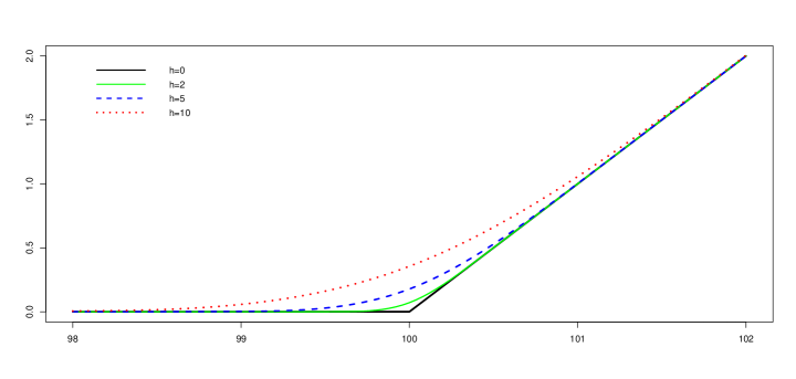
Panel B: Option Payoff Derivative $Dg_{k}^{h}(X)$

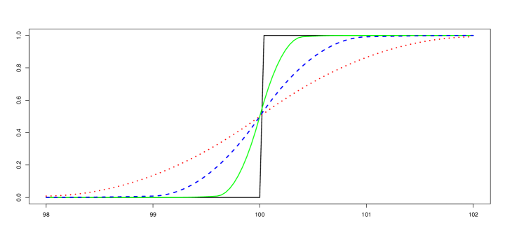
Panel C: Smooth Superhedging

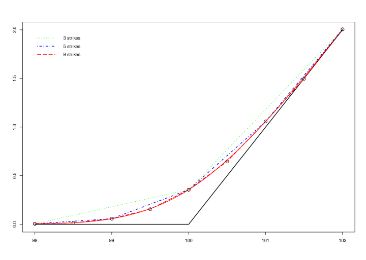
Figure 1. Smoothing Option Payoff by $h$.
Plot of $g_{k}^{h}(x)$ (Panel $A$) and $Dg_{k}^{h}(x)$ (Panel $B$) for $k=100$ and $h=2,5,10$. In Panel C we draw $g_{k}^{h=10}(x)$ (red dotted line) together with $\hat{g}_{k}^{h=10}(X)$ (piecewise linear curves), the payoff of the portfolio superhedging it assuming to have 3, 5 or 9 equally spaced strike prices.

In Panel C the target payoff $g_{k}^{h}$ is plotted together with the payoff $\hat{g}_{k}^{h}$ of the portfolio that super replicates it in order to understand the role of efficiency. By construction, superhedging $g_{k}^{h}$ or $\hat{g}_{k}^{h}$ are entirely equivalent exercises. Thus, the degree of smoothness involved depends not only on the shape of the notional payoff $g_{k}^{h}$ but also on that of its market counterpart, $\hat{g}_{k}^{h}$, and particularly on the number of contracts involved in superhedging. This remark highlights the role of the bandwidth $h$. A small value of this parameter makes the width of the smoothing interval $[k-h,k+h]$ narrow and diminishes, as a consequence, the distance between $g_{k}^{0}$ and $g_{k}^{h}$, as shown in Lemma 1. At the same time the number of efficiently priced options with strike price included in such interval – i.e. the size of the set $[k-h,k+h]\cap K^{0}(X)$ – is reduced, making the super hedging payoff $\hat{g}_{k}^{h}$ less smooth. In fact, in Panel C – with $6$ equally spaced efficient strike prices ranging from $95$ to $105$ – the payoff $g_{k}^{h}$ is represented by a continuous, smooth line while $\hat{g}_{k}^{h}$ is the piecewise linear curve of the same color dominating it. In the case $h=2$, the super hedging portfolio only contains $2$ options while for the case $h=10$ it contains all $6$. It is clear from the picture that $\hat{g}_{k}^{h}$ becomes less smooth as it approaches $g_{k}^{0}$, suggesting the need to balance these two countervailing effects.

To understand this point better, let $M$ be the mesh of $K(X)\setminus\{0\}$, i.e.

(22) $$M=\sup\big{\{}|k-k^{\prime}|:k,k^{\prime}\in K(X)\setminus\{0\},\ k\neq k^{\prime}\big{\}}$$

and $M^{0}$ the mesh of $K^{0}(X)\setminus\{0\}$. Let also $w_{k}^{h}(j)$ denote the quantity invested in option $\theta(j)$, with $j\in K^{0}(X)$, in order to super hedge $g_{k}^{h}$, obtained from (6). From the fact that $g_{k}^{h}$ and $g_{k}^{0}$ coincide outside of the interval $[k-h,k+h]$ by (17) and from (6) we deduce the implications

(23a) $$w_{k}^{h}(j_{i})>0\quad\Rightarrow\quad j_{i+1}+h>k>j_{i-1}-h\quad\Rightarrow\quad|k-j_{i}|<h+M^{0}\qquad i=1,\ldots,I$$

(23b) $$w_{k}^{h}(0)>0\quad\Rightarrow\quad j_{1}>k-h$$

This suggests to set $h=\delta M$ so to make the properties of the estimator sample dependent. In the sequel we will replace the superscript $h$ with $\delta$. We observe that, as a consequence of (23), the number of efficient options employed in order to superhedge $g^{\delta}_{k}$ is at most $3+2\delta M/M^{0}$ so that it is desirable to fix $\delta>M^{0}/M\geq 1$ in order to have at least $5$ options available. In the following sections we will experiment values of $\delta$ ranging from $1$ to $10$.

3.2. Properties of the Estimator

A different and more classical question is whether the proposed estimator converges to the true price function in the presence of disturbances. The classical formulation of this problem is

(24) $$q(k)=F(k)+\varepsilon_{k}\qquad k\in K(X)$$

where $F$ is the model, and is thus assumed to be a positive, decreasing, convex, $\mathscr{C}^{2}$ function, whereas the errors $\varepsilon_{i}$ are identically and independently distributed with zero expectation.

Theorem 1 gives an explicit functional form to our estimator:

(25) $$q^{\delta}(k)=\sum_{j\in K^{0}(X)}w_{k}^{\delta}(j)q(j)\qquad t>0$$

Observe that, by (37) and Assumption 2,

(26) $$w_{k}^{\delta}(j)\geq 0\quad\text{for all}\quad j\in K^{0}(X)\quad\text{and}\quad\sum_{j\in K^{0}(X)}w_{k}^{\delta}(j)=1$$

At first sight, then, our estimator appears as an exemplification of the local averaging approach which includes, as additional special cases, kernels and regressograms. For this class of estimators a well established theory demonstrates (see e.g. [25, p. 677]) that the MSE converges to $0$ as the sample size diverges. However, in local average estimators weights are assumed to be uncorrelated with disturbances and this is of crucial importance in proving convergence. In our setting, instead, this property can in no way be assumed to hold. In fact the set $K^{0}(X)$ of efficient option prices, hitherto treated as given, will in general strongly depend on prices and therefore on disturbances. Not only but the inclusion of a given price $k$ in $K^{0}(X)$ will depend not only on the corresponding noise but also on all other disturbances since a high value for $\varepsilon_{k^{\prime}}$ will make it more likely for $q(k)$ to be efficient. The problem discussed provides a clear exemplification of the selection bias studied by Heckman [15] and it is to some extent surprising that its pervasive role in empirical option pricing has not been fully recognized. From the classical work of Heckman we learn, in fact, that selection effects may result in biased and inconsistent estimates unless correcting for a term which proxies the expected value of disturbances conditional on selection. The work of Heckman has been extended to the non parametric setting in a recent paper by Das et al. [7]. Our aim is that of giving sufficient conditions for the $MSE$ to converge to $0$ when taking the selection effect fully into account.

The first step is to treat $K^{0}(X)$ as a random variable. Observe to this end that the inclusion $k\in K^{0}(X)$ holds if and only if the $\mathscr{F}$ measurable event $A_{k}=\{q(k)\leq q^{0}(k)\}$ occurs. In order to take randomness into full account we replace the symbol $K^{0}(X)$ with $Z(\omega)\subset K(X)$. Then, if $z\subset K(X)$ we have that $\{Z=z\}=\bigcap_{k\in z}A_{k}\in\mathscr{F}$. We observe that although the value of $w_{k}^{\delta}(j)$ depends crucially on $Z$, it is in fact deterministic once conditional on the event $\{Z=z\}$. It is thus natural to follow a two step procedure (similarly to Heckman and to Das et al.) by first conditioning all variables on the selection mechanism and then focusing on the unconditional properties. Denote by $P_{z}(\cdot)$ the conditional expectation given the event $\{Z=z\}$, for $z\subset K(X)$ and $P_{Z}(\cdot)=\sum_{z\subset K(X)}P_{z}(\cdot)\mathbf{1}_{\{Z=z\}}$. When needed we explicit $z$ as $\{0=j_{0}^{z}<j_{1}^{<}\ldots<j_{I^{z}}^{z}\}$ and write

$$\tau_{i}=\sum_{z\subset K(X)}j_{i}^{z}\mathbf{1}_{\{Z=z\}}$$

Denote by $M_{z}$ and $M_{Z}$ the mesh of the sets $z\setminus\{0\}$ and $Z\setminus\{0\}$ respectively. The variable $P_{Z}(\varepsilon)$ will be our correction term.

Theorem 3.

Let the function $F:\mathbb{R}_{+}\to\mathbb{R}_{+}$ in (24) be decreasing and convex and assume that $F\in\mathscr{C}^{3}$ with $\sup_{x\in\mathbb{R}_{+}}|D^{3}F(x)|<\alpha$. Assume moreover that

(27a) $$E(\varepsilon_{\tau}\varepsilon_{\sigma})=0,\quad P_{Z}(\varepsilon_{\tau})=P_{z}(\varepsilon_{\sigma})\quad\text{and}\quad P_{Z}(\varepsilon_{\sigma}\varepsilon_{\tau})=P_{z}(\varepsilon_{\sigma^{\prime}}\varepsilon_{\tau^{\prime}})\qquad\text{for all}\quad\sigma,\tau,\sigma^{\prime},\tau^{\prime}\in Z$$

(27b) $$E\Big{(}\sup_{\tau\in Z}P_{Z}(|\varepsilon_{\tau}|)\Big{)}<\infty\quad\text{and}\quad E\Big{(}\sup_{\sigma,\tau\in Z}P_{Z}(|\varepsilon_{\sigma}\varepsilon_{\tau}|)\Big{)}<\infty$$

(27c) $$\lim_{M\to 0}E\big{(}M_{Z}^{6}\big{)}=0\quad\text{and}\quad\lim_{M\to 0}P(\tau_{1}>0)=0$$

Then, for any compact interval $I\subset\mathbb{R}_{+}\setminus\{0\}$

(28) $$\lim_{M\to 0}\sup_{t\in I}E\Big{(}\big{(}q^{\delta}(t)-F(t)\big{)}^{2}\Big{)}=0$$

Condition (27a) is conceptually akin to the assumption made by Das et al. that the conditional expectation of the disturbance given selection depends only on the propensity score, see [7, Assumptions 2.1, 2.2 and 2.3]. Condition (27b) is easily satisfied if, e.g., disturbances are uniformly distributed. The the most delicate property is definitely (27c) as it requires a strong form of convergence to $0$ of the mesh of $K^{0}(X)$. The proof of Theorem 3 strongly relies on some properties of the smoothing spline $g_{k}^{\delta}$ proved in Lemma 1, a fact emphasizing the role of splines.

3.3. The density approach

As mentioned in the introduction, splines are not the only possible choice for smoothing option payoff. We present in this paragraph an alternative based on some given probability density function, $\phi$, satisfying the properties

(29) $$\int u\phi(u)du=0\quad\text{and}\quad\int|u|\phi(u)du<\infty$$

Denote by $\Phi$ the distribution function associated with $\phi$ and consider the following function:

(30) $$g_{k}^{h}(x;\phi)=\Phi\Big{(}\frac{x-k}{h}\Big{)}(x-k)-h\int_{-\infty}^{(x-k)/h}u\phi(u)du$$

Lemma 2.

Let $\phi$ be a probability density function satisfying (29). Then the function $g_{k}^{h}(\cdot;\phi)$ defined in (30) satisfies properties (i), (ii) and (iii) of Lemma 1.

The proof of the Lemma is rather clear given the explicit form of the derivatives of $g_{k}^{h}(x;\phi)$, i.e.

(31) $$Dg_{k}^{h}(x;\phi)=\Phi\Big{(}\frac{x-k}{h}\Big{)}\quad\text{and}\quad D^{2}g_{k}^{h}(x;\phi)=\phi\Big{(}\frac{x-k}{h}\Big{)}\frac{1}{h}$$

in which it is implicit the inequality

$$0\leq g_{k}^{h}(x;\phi)-g_{k}^{0}(x)\leq g_{k}^{h}(k;\phi)-g_{k}^{0}(k)\leq h\int|u|\phi(u)du$$

A special case of (30) is given by the standard normal distribution:

(32) $$g_{k}^{h}(x;\mathscr{N})=\Phi_{\mathscr{N}}\Big{(}\frac{x-k}{h}\Big{)}(x-k)+h\phi_{\mathscr{N}}\Big{(}\frac{x-k}{h}\Big{)}$$

that will be briefly considered in the applications that follow, as a term of comparison.

A noteworthy implication of (30), emerging clearly from (31) and (4), is the possibility to extract from the non parametric prices $q^{h}(k;\phi)$ an implicit risk neutral density in closed form, that is

(33) $$d^{h}(x;\phi)=\sum_{i=1}^{I}b_{i}D^{2}g_{j_{i}}^{h}(x;\phi)=\sum_{i=1}^{I}b_{i}\phi\Big{(}\frac{x-j_{i}}{h}\Big{)}\frac{1}{h}$$

where the parameters $b_{i}$ are the positive coefficients in (6). The implicit risk neutral density belongs thus to a preassigned family of density mixtures without actually having to make this assumption but rather as the consequence of the exact market pricing of a specific class of derivatives, $g^{h}_{k}(\phi)$. Not only, but the mixing parameters are fixed by the market so that in order to estimate the implied risk neutral density one only has to specify the bandwidth $h$.

In the option pricing literature a lot of interest was raised by models which assume that the risk neutral density is a mixture of log normals. This modeling choice has been adopted, among others, by Ritchey [20], Melick and Thomas [19], Söderlind and Svensson [23] and Söderlind [22]. In [22], Söderlind lists among the advantages of this approach the closed form for option prices and the flexibility of this family of densities which easily accommodates for skewness and kurtosis of returns while avoiding the difficulties inherent in the non parametric approach. Although this is clearly not the focus of our work, we mention however the relative ease of (33) in which the weights $b_{i}$ are in fact fixed by the market and do not have to be estimated, which is typically a delicate step involving the EM algorithm. In the next section we confront the implicit density (33) with the true one when it is assumed that the returns follow a mixture of log normals to provide at least some evidence that our approach is a viable solution for those cases in which the assumption of a mixture of log normals is justified.

4. Empirical Applications: Simulation Analysis

In this section we are going to test our methodology using as our benchmark the classical model of Black and Scholes, augmented for smile effects, using exactly the same values as in Aït-Sahalia and Duarte [1] for ease of comparison. The current underlying price is set at $1,365$, maturity to 3 months, the interest rate at $4\%$ and we assume no dividends. We consider 25 strike prices equally spaced between $1,000$ and $1,700$, so that $M=28$. Volatility will be a linear, decreasing function of the strike, ranging from $40\%$ to $20\%$. With these values, the option prices range from $378$ to $0.9$.

4.1. Deterministic Analysis

As a first step in our analysis we investigate how close are the quantities $q^{\delta}(k)$, $\sigma^{\delta}(k)$ and $\nu^{\delta}(X>k)$ to the true values computed from the model, where $\sigma^{\delta}(k)$ is the the level of volatility implicit in $q^{\delta}(k)$ according to the Black and Scholes formula. We experiment three possible values of the smoothing parameter, namely $\delta=2,5,10$. The results, in terms of deviations of estimated values from true ones, are plotted in Figure 2. Panel $A$ represents the price gap, Panel $B$ the volatility gap and Panel $C$ the gap in terms of cumulative probability. For all choices of $\delta$, the distance between true and fictitious values appear to be rather small. Deviations of the smooth price from the true one are indeed quite limited but contain a smile effect and increase for options out of the money. This phenomenon, quite limited, soon disappears when we move from $\delta=10$ to $\delta=5$. Deviations from the benchmark are more interesting when considering the implicit probability as the smooth functions lie below $0$ up to $1,460$ for all choices of $\delta$.

Panel A: Option Price $q^{\delta M}(k)$

Panel B: Implied Volatility

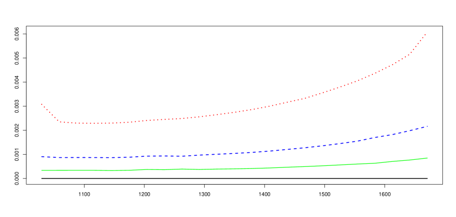
Panel C: Probability $\nu^{\delta M}(X>k)$

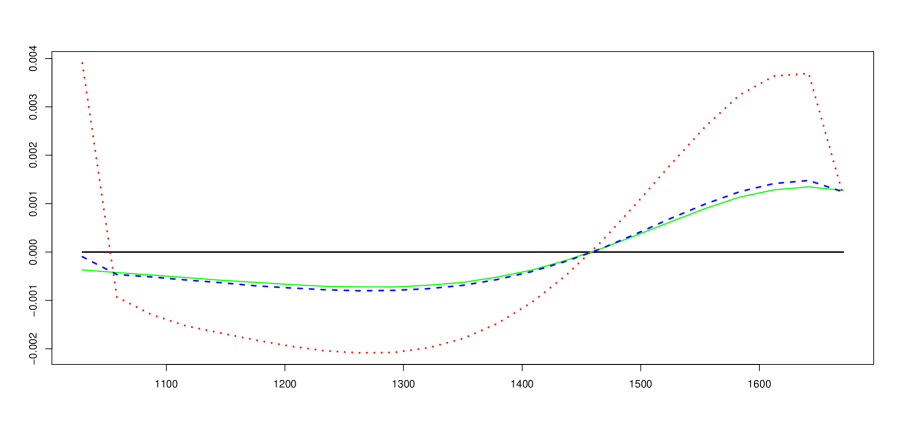
Figure 2. Deviations from Black and Scholes with a Smile.
$\sigma=0.4-0.2(k-1000)/700$, $\nu^{B\&S}=-\partial q^{B\&S}\left/\partial K\right.-\partial q^{B\&S}\left/\partial\sigma\right.d\sigma\left/dk\right.$ and $N=10$.

4.2. Smoothness vs. Variance

The picture changes significantly as we introduce noise into the original model. To avoid arbitrariness we still follow Aït-Sahalia and Duarte [1]. In particular we believe that noise has an implicit microstructural component that may be well captured by liquidity and the bid/ask spread. We proxy illiquidity of options via the factor $1+5|\exp(r\tau)k/S_{0}-1|$ which is 1 for options exactly at the money and gets as high as $2.3$ for deeply in and out of the money options. We fix the basis spread to $5\%$ of the option price with a floor at $50$ cents and a cap at $3$ dollars. Noise is then modeled as a random variable which is uniformly distributed on an interval centered at the origin and with radius equal to the product of illiquidity and half of the spread.

In Figure 3 we draw the distance between the correct Black and Scholes price and its estimate $q^{\delta}(k)$ when prices are affected by errors, in the way described above.

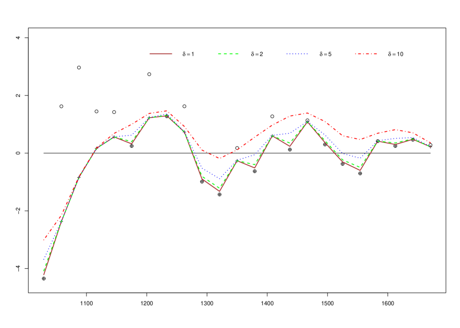
Figure 3. Smoothness vs. Variance.
Estimating the model $q(k)+\varepsilon_{k}$ with $N=10$ and $\delta=1,2,5,10$. Values are expressed in terms of their distance from the correct B&S price. Actual option prices are plotted as circles while the corresponding efficient prices are plotted as crosses. The two symbols are overwritten whenever the corresponding strike belongs to $K^{0}(X)$.

The picture shows that the higher the value of $\delta$ the more smooth is the resulting estimate while, at the same time, goodness of fit decreases. This is a classical finding in non parametric statistics but presents here some new feature. We observe first that non efficient option prices, corresponding to plain circles, have actually no impact on estimates. The corresponding superhedging prices are plotted as crosses (so that the superposition of a cross to a circle signifies that the corresponding strike is an element of $K^{0}(X)$). $8$ prices out of $24$ are non efficient and, as can be seen, most of them are concentrated on the left-hand side corresponding to deeply ITM options. This is due to the combined effect of illiquidity and of the spread which, in our set-up as in the real world, magnifies noise for this segment of the options market. We remark that noise has an asymmetric effect. A positive shock, particularly in the presence of a strong microstructural multiplier, will make the corresponding price inefficient and thus has no impact on our estimates. If the shock is negative or small in magnitude then it is less likely to produce price inefficiency and will be included in the estimated values. Our method is subject to a limited underestimation error for those prices which are affected by errors in a more relevant way,as is the case here for options deeply ITM. Second, we notice that the higher is $\delta$ the more upward shifted will be the fitting curve. This follows from the payoff $g_{k}^{\delta}$ being larger. Including a constant term to the estimated CALL function would indeed reduce this problem as long as the constant make take on either sign. This addition would correspond however, in its financial counterpart, to the possibility of taking long or short positions in the riskless asset, a modeling choice which, although completely standard in the literature, blatantly contrasts with our starting assumptions.

4.3. Monte Carlo Simulation

In order to construct interval estimates and evaluate the statistical aspects of our approach we run $5,000$ Monte Carlo simulations of the error terms. Our model takes the form

(34) $$q(k)+\varepsilon_{k}^{s},\qquad k\in K(X),\ s=1,2,\ldots,5000$$

where the error terms are distributed as described above.

	dITM	ITM	ATM	OTM	dOTM	Total
Nr	6	5	5	4	5	25
mean	52.12	50.8	30.5	18.0	15.32	34.74
min	0.0	0.0	0.0	0.0	0.0	12.0
max	83.33	80.0	80.0	75.0	60.0	56.0

Table 1: Percentage of inefficient prices for each market segment.

The introduction of noise produces a number of arbitrage violations, as documented in the preceding Table 1. These violations amount on average to $34.74\%$ of the sample but range up to $56\%$ and are above $40\%$ in the $20\%$ of cases.

For any simulation $s=1,\ldots,5000$ we compute, via Theorem 1, the corresponding CALL function, $q^{\delta,s}(k)$, implied volatility , $\sigma^{\delta,s}(k)$, and the associated probability $\nu^{\delta,s}$ for different values of $h$, although we only plot $\delta=5,10$. For each strike price $k$, we then compute the mean and the quantiles of the simulated sample obtaining for each quantity of interest maximum and minimum values, $90\%$ and $95\%$ confidence intervals, mean and standard deviation. The corresponding curves are plotted in Figure 4, for $\delta=5$, and Figure 5, for $\delta=10$.

We notice that, although in the worst possible scenarios the most deeply ITM options may be overpriced or underpriced by almost $5$ $ (when the price fixed by the model is however more than $300$ $), the mean pricing error is never larger than $2$ $ and, for reasonably liquid options just a few cents. Second, illiquid options are on average underpriced because of the effect highlighted before by which our method makes mainly use of prices affected by negative error terms. This may be considered as an asymmetric smile effect resulting, however, from microstructural factors.

Panel A: Option Price

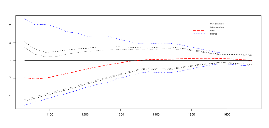
Panel B: Volatility

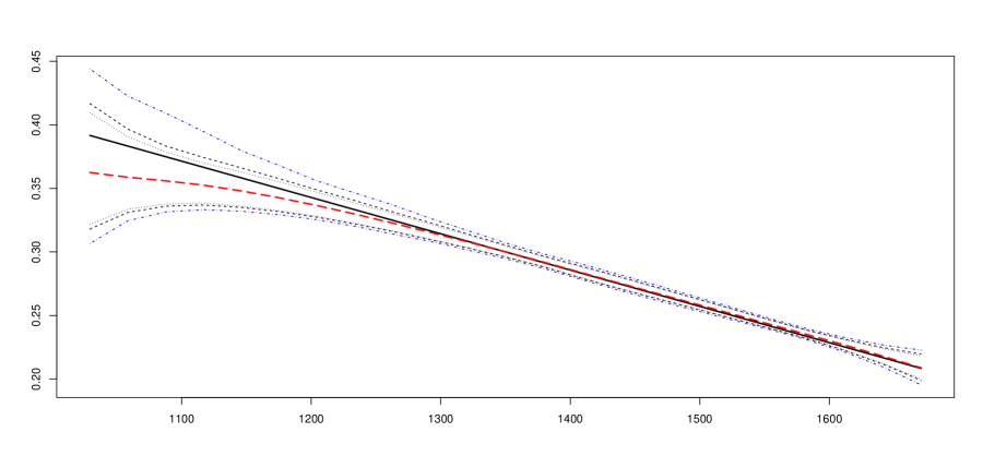
Panel C: Probability

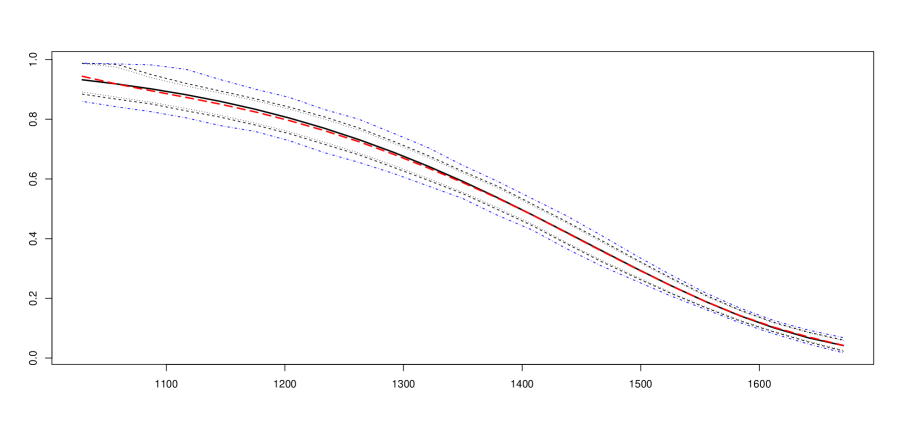
Figure 4. Simulated Simulated Confidence Intervals: $N=10$ and $\delta=5$.
The confidence bands and mean were obtained after $5,000$ Monte Carlo simulations.

Panel A: Option Price

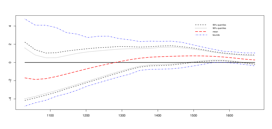
Panel B: Volatility

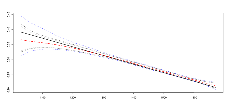
Panel C: Probability

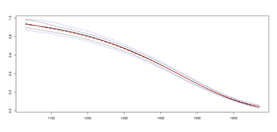
Figure 5. Simulated Confidence Intervals: $N=10$ and $\delta=10$.
The confidence bands and mean were obtained after $5,000$ Monte Carlo simulations.

It is noteworthy that for $\delta=5$ the true value always falls inside the confidence interval even at the $90\%$ level for all three variables considered, suggesting that our approach produces quite reliable predictions. One may also notice that the two confidence bounds are not symmetric, especially for options deep in the money, reflecting the same distortion noted above. For the case $\delta=10$ the situation partly changes as the estimate of the option price becomes less precise and, in particular, the mean price exceeds the actual one by more than 50 cents for all options ATM or OTM. In addition, both lower confidence bounds are breached as frequently as $21.7\%$ suggesting that the choice $\delta=10$ produces an increase in smoothness which results however in a significant pricing error. We investigated also the results relative to the intermediate values of $\delta$ and we report the corresponding values of the mean squared error

(35) $$MSE=\frac{1}{5,000\times 24}\sum_{k\in K(X)}\sum_{s=1}^{5,000}\big{(}q^{\delta,s}(k)-q(k)\big{)}^{2}$$

which we report in Table 2.

	$N=4$	$N=6$	$N=8$	$N=10$
$\delta=1$	1.93	1.99	2.02	2.03
$\delta=2$	1.78	1.87	1.92	1.95
$\delta=5$	1.61	1.63	1.72	1.76
$\delta=10$	6.17	2.06	1.61	1.58

Table 2. Values of the MSE for alternative parameter choices.

In the literature there is greater emphasis on the implied risk neutral density rather than on the implicit probability so that the focus is actually on the second derivative of the CALL function. We do not have a special interest for this quantity here, partly because the presumption that a density actually exists has no financial basis. In part, however, it is our choice to work with cubic splines that limits our ability to explore densities. Second derivatives in fact exist but are piecewise linear, making the candidate density function not particularly interesting for applications. To obtain smoothness of the implied risk neutral density one should perhaps adopt a different functional form than cubic splines such as splines of higher order (which are however much less tractable computationally speaking) or as the normal option smoother described in (32). Another possibility would be to apply to the density obtained some local smoothing technique. In the Monte Carlo analysis performed here, however, smoothness of the density function arises upon averaging across all simulations. In Figure 6 we plot the estimated mean density function together with the one originated from model. The value for the MISE so obtained is $4.402242e-07$ and $4.318549e-07$, for $\delta=5$ and $\delta=10$ respectively.

Panel A: $\delta=5$

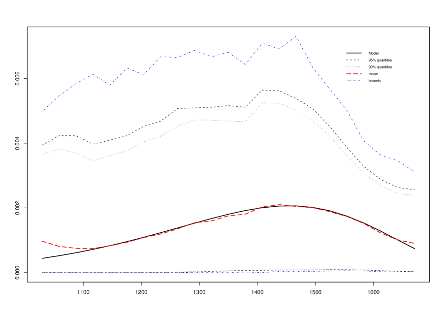
Panel B: $\delta=10$

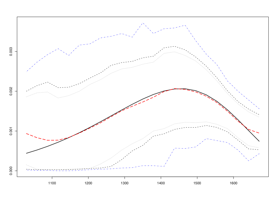
Figure 6. Implied risk-neutral average density: $N=10$ and $\delta=5,10$.

4.4. A word on normal option smoothing.

We have performed the above analysis also via the normal options smoothing formula (32) rather than splines. The resulting values for the MSE as well as of confidence levels are less satisfactory than those reported above. We claim, however, that,in models assuming that the risk neutral density is a mixture of log-normals, then the density approach described in (32) produces remarkable results. To this end we have considered three normal densities with instantaneous parameters $\mu=\{0.027,0.033,0.049\}$ and $\sigma=\{0.3,0.1,0.4\}$ and weights $\alpha=\{0.2,0.3,0.5\}$, respectively. We have used the same values for strike prices, underlying, maturity and interest rate as above. Given these values, we obtain risk neutral prices for options with strike prices ranging from 1,000 to 1,700. From such prices we extract the implied risk neutral density by using (32) after setting $h=20$. We plot in Figure 7 the conditional risk-neutral densities over the interval $1,050-1,650$. We stress that indeed the mixture of log-normals is rather fat tailed, as desired, but also that its non parametric estimate is indeed very close to it. The corresponding value for the MISE amounts to $3.34864e-06$.

Risk neutral density

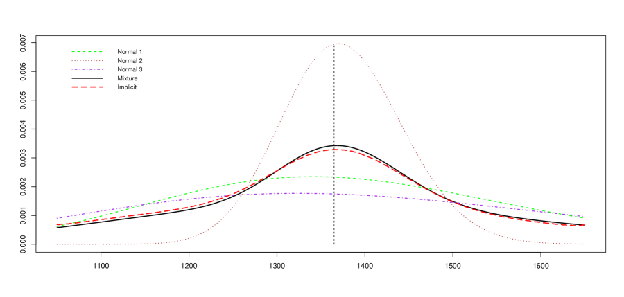
Figure 7. Risk-neutral densities for a mixture of log-normals.
All curves represent a corresponding conditional density over the interval $1050-1650$. The dashed lines are the starting log-normal densities and the black solid line their mixture. The red line is the density extracted from the option prices. $MISE=3.34864e-06$.

5. Empirical Applications: Market Data

Eventually, we consider an application to market data by selecting an arbitrary trading day, 21^st October 2010, on the S&P 500 options market. We sample ask quotes at time intervals of one minute each and disregard quotes for which the reported ask size is below 100. On the subsample so obtained we have options quotes for 180 different strike prices – ranging from 50 to 2500 – and 12 possible maturities – from $22^{nd}$ October 2010 to $22^{nd}$ December 2012. We focus on options expiring in November 2010 and their quotes at 12:06, 12:39 and 13:03, around the market downturn of Figure 8.

Figure 8. The S&P 500 Index on 21^st October 2010

At the three selected times and for the selected maturity there are 65, 53 and 67 efficiently quoted strike prices respectively out of 90, 75 and 99. We therefore have a relatively long cross section of strikes and an incidence of inefficient prices of $30\%$ on average. The large number of available strikes is one of the advantages of working with quoted ask prices, as dictated by our model, rather than transaction prices. In the sample there is an overwhelming ratio of contracts ITM by $10\%$ or more and virtually no OTM contract as reported in Table 3.

	Total	dITM	ITM	ATM	OTM	dOTM
Sample	23.972	45.53	27.15	27.22	0.09	0
12:06	90	39.77	35.23	25.00	0	0
12:39	75	52.31	32.31	15.38	0	0
13:03	99	38.37	31.39	30.23	0	0

Table 3: Contracts by Moneyness, $S_{t}/K$.

We select a subsample of strikes ranging from 670 to 1,255. At 12:39 the lesser number of strikes quoted corresponds to a larger maximum interval between consecutive strikes, i.e. $M=70$, while at the other moments strikes do not differ by more than 25 and 30, respectively. Thus for the typical choice $\delta=5$ we expect to have a relatively poor performance at $12:39$, due to the high value of $M$. In the following picture we plot for each time $t$ the curves corresponding to the three distinct values of $\delta=2,5,10$.

Panel A: Option Prices at 12:06

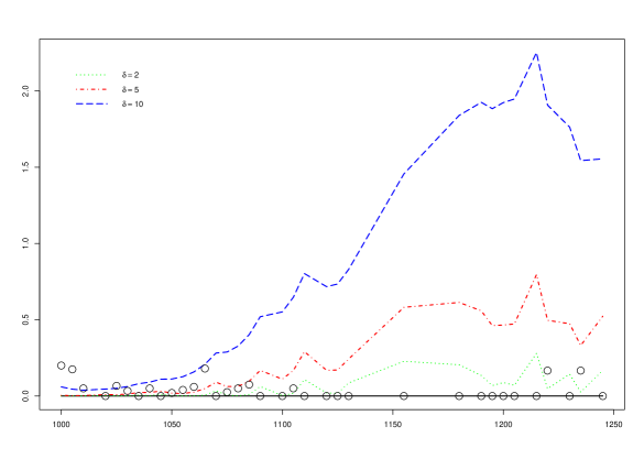
Panel B: Option Prices at 12:39

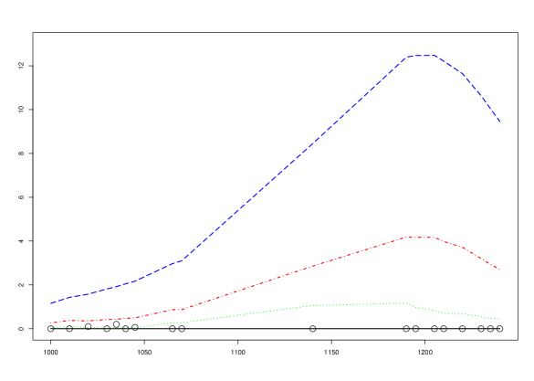
Panel C: Option Prices at 13:03

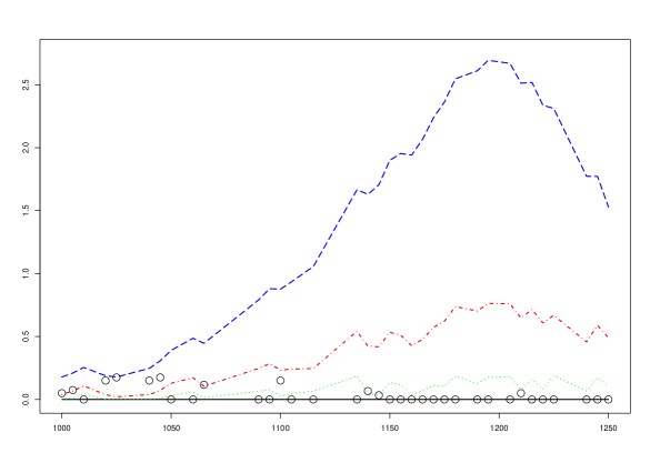
Figure 9. Actual and estimated option prices as differences with the efficient prices. Market prices are represented as circles.

In fact we clearly see from Figure 9 that the performance of our estimates at $12:39$ is quite poor due to the fact that there is just one quoted strike between 1075 and 1175. The price curve ends up being very smooth but overestimates actual prices by as much as $5\$$ for the value $\delta=5$ while in the other selected instants the price gap never exceeds $50$ cents for such a parameter choice.

Eventually we plot, for the value $\delta=5$, the implied conditional risk neutral probability and density at $12:06$ and $13:03$, Figure 10, to capture the effect of the market downturn on $\nu^{\delta}$ and $d^{\delta}$. As expected, the fall in the underlying price determines a more pessimistic view embodied in the implied risk neutral distribution. Of course, as explained above, the density is not a smooth quantity, due to our choice of working with cubic splines.

Panel A: Implied risk neutral probability

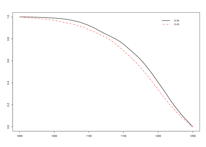
Panel B: Implied risk neutral density

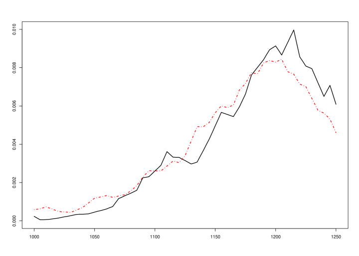
Figure 10. Conditional risk neutral distribution, $\nu^{\delta}(X>x)$, and density, $d^{\delta}(x)$, at 12:06 and 13:03 for the case $\delta=5$.

Eventually, we can use the above information to compute some measures of risk. In particular we consider a long position in a future contract expiring on November 2010, i.e. in a month. The future price is set according to the future/spot parity, $F(t,T)=S_{t}\exp(r(T-t))$. As a proxy for the riskless rate $r$ we use the 1 month LIBOR rate on that date, quoted at $3.96\%$. We then compute the $VaR$ and conditional $VaR$ at a confidence level of $2\%$ and $5\%$ at the two instants of time. The values are reported in the following Table 4:

	2.5%	5%
$VaR$ 12:06	177.58	110.08
$VaR$ 13:03	163.94	123.95
$CVaR$ 12:06	183.00	134.30
$CVaR$ 13:03	171.26	149.65

Table 4: Measures of risk.

These last remarks suggest the importance to investigate the dependence of $\nu$ on the current value of the underlying, although outside of our interests here. Another issue that would be important to address is the time evolution of the pricing measure.

Mathematical Appendix

In this appendix we present some results which we used in the proofs of the main Theorems.

Results from section 2

Proof of Theorem 1.

The claim essentially follows from [6, Lemmas 7 and 8] in which, however, it is assumed that $x<\infty$. The proof given here is adapted from that one to cover the present setting. First of all, in superhedging a given claim, we can restrict to the options which are priced efficiently, i.e. whose strike is included in $K^{0}(X)$. Let $j_{0}=0$ and write $j_{I+1}=x$, if $x<\infty$ or else $j_{I+1}>j_{I}$ arbitrarily. $g^{0}_{\theta}(X)\geq f(X)$ for $X=0$. Assume that $g_{\theta}^{0}(j_{i})<f(j_{i})-\varepsilon$ for some $i=1,\ldots,I+1$. By continuity there exists then $\delta>0$ such that $g^{0}_{\theta}(X)<f(X)-\varepsilon$ holds on the set $\{j_{i}-\delta<X\leq j_{i}\}$. However, $P(j_{i}-\delta<X\leq j_{i})>0$ since otherwise $\mathrm{ess}\sup(X\wedge j_{i})\leq j_{i}-\delta$ in contrast with Assumption 1. Thus $g^{0}_{\theta}(X)\geq f(X)$ a.s. implies that $g^{0}_{\theta}(j_{i})\geq f(j_{i})$ for $i=0,\ldots,I+1$. If $\bar{X}=\infty$ then by the fact that $j_{I+1}$ was chosen arbitrarily we deduce $g^{0}_{\theta}(x)/x\geq f(x)/x$, i.e. $1\geq\hat{f}(\bar{X})$.

Viceversa, if $g_{\theta}^{0}(j_{i})\geq f(j_{i})$ for $j=0,\ldots,I+1$, then for each $\omega\in\{X\leq\bar{X}\}$ and some choice of $j_{I+1}$ there exists $i(\omega)\in\{0,1,\ldots,I\}$ such that, for some $0\leq a\leq 1$, $j_{i(\omega)}\leq X(\omega)\leq j_{i(\omega)+1}$ and thus

$$f(X(\omega))\leq af(j_{i(\omega)})+(1-a)f(j_{i(\omega)+1})\leq ag_{\theta}^{0}(j_{i(\omega)})+(1-a)g_{\theta}^{0}(j_{i(\omega)+1})=g^{0}_{\theta}(X(\omega))$$

because $f$ is convex and $g^{0}_{\theta}$ is linear on each interval $[j_{i},j_{i+1}]$. In other words, $g^{0}_{\theta}(X)\geq f(X)$ outside of $\{X>\bar{X}\}$ i.e. $P$-a.s. so that the inequality $g^{0}_{\theta}(X)\geq f(X)$ $P$-a.s. may be written in vector notation as

$$\mathbf{D}\mathbf{a}\geq\mathbf{f}$$

where $\mathbf{a}$ is the vector of weights $a_{1},\ldots,a_{I}$ such that $\theta=\sum_{i=1}^{I}a_{i}\theta(j_{i})\in\Theta$, $\mathbf{D}$ is the $(I+1)\times(I+1)$ matrix whose inverse appears in (4) and $\mathbf{f}=[f(j_{1}),\ldots,f(j_{I}),\hat{f}(\bar{X})]^{T}$.

Define the vectors $\mathbf{w},\mathbf{b}\in\mathbb{R}^{I+1}$ implicitly by letting

(36) $$b_{I}d_{I}=q(j_{I})\quad\text{and}\quad b_{I}e_{I}+\sum_{i=n}^{I-1}b_{i}=\frac{q(j_{n})-q(j_{n+1})}{j_{n+1}-j_{n}}\qquad n=0,\ldots,I-1$$

with $e_{I}=1$ if $\bar{X}<\infty$ or else $e_{I}=0$ and

(37) $$\sum_{i=0}^{n}w_{i}=\frac{f(j_{n+1})-f(j_{n})}{j_{n+1}-j_{n}}\qquad n=0,\ldots,I-1\quad\text{and}\quad\sum_{i=0}^{I}w_{i}d_{i}=\hat{f}(\bar{X})$$

Clearly, $w$ and $b$ satisfy (6). The following properties are easily established by induction: (i) $\mathbf{b}\geq 0$ (as $j_{0},\ldots,j_{I}\in K^{0}(X)$), (ii) $\mathbf{w}\geq 0$ (as $f\in\Gamma$), (iii) $\mathbf{b}^{T}\mathbf{D}=\mathbf{q}^{T}$ and (iv) $\mathbf{w}=\mathbf{D}^{-1}\mathbf{f}$. But then,

$$q(\theta(f)) =\min_{\left\{\mathbf{a}\in\mathbb{R}^{I+1}_{+}:\mathbf{D}\mathbf{a}\geq\mathbf{f}\right\}}\mathbf{q}^{T}\mathbf{a}=\min_{\left\{\mathbf{a}\in\mathbb{R}^{I+1}_{+}:\mathbf{D}\mathbf{a}\geq\mathbf{f}\right\}}\mathbf{b}^{T}\mathbf{D}\mathbf{a}\geq\mathbf{b}^{T}\mathbf{f}=\mathbf{q}^{T}\mathbf{w}$$

∎

Results from section 3

Proof of Lemma 1..

By a result of Turlach [24, p. 85] the program (16) admits as its solution a cubic $\mathscr{C}^{2}$ spline of the form

$$g_{k}^{h}(x)=\sum_{i=1}^{N}\mathbf{1}_{\big{[}k+t^{h}_{i},k+t^{h}_{i+1}\big{)}}(x)\Phi_{k,i}^{h}\Big{(}x-(k+t^{h}_{i})\Big{)}+\mathbf{1}_{\big{[}k+t^{h}_{I},\infty\big{)}}(x)(x-k)\qquad x\in\mathbb{R}_{+}$$

where $t_{1}^{h},\ldots,t_{N+1}^{h}$ are as in the text and $\Phi^{h}_{k,i}$ is a polynomial of degree $3$ for $i=1,\ldots,I$. It is clear from the constraints imposed to (16) that indeed $g_{k}^{h}\in\Gamma$. Moreover, these same constraints imply that $g_{k}^{h}(x)=g^{0}_{k}(x)$ when $x\notin[k-h,k+h]$ while $1\geq Dg_{k}^{h}(x)\geq 0$ on $[k-h,k+h]$. Thus, $g_{k}^{h}-g^{0}_{k}$ is increasing on $(-\infty,k]$ and decreasing afterwards, so that $\sup_{x}(g^{h}_{k}-g^{0}_{k})(x)\leq(g^{h}_{k}-g^{0}_{k})(k)=g^{h}_{k}(k)$. Moreover, the (non empty) set of solutions is clearly convex and the functional $I_{k}(h;f)$ is strictly convex in $f$ so that the solution is necessarily unique. Define

$$\bar{g}_{k}^{h}(x)=g_{k}^{h}(2k-x)+(x-k)\qquad x\geq 0$$

and observe that $\bar{g}_{k}^{h}\in\chi(k;h)$. Moreover, one deduces from (15) that

$$I_{k}(h;\bar{g}_{k}^{h}) =\sum_{i=1}^{N+1}\big{[}g_{k}^{0}(k+t_{i}^{h})-\bar{g}_{k}^{h}(k+t_{i}^{h})\big{]}^{2}+(0.1h)^{3}\int_{k-h}^{k+h}\big{(}D^{2}\bar{g}_{k}^{h}(x)\big{)}^{2}dx$$

$$=\sum_{t_{i}^{h}\leq 0}\big{[}\bar{g}_{k}^{h}(k+t_{i}^{h})\big{]}^{2}+\sum_{t_{i}^{h}>0}\big{[}\bar{g}_{k}^{h}(k+t_{i}^{h})-t_{i}^{h}\big{]}^{2}+(0.1h)^{3}\int_{k-h}^{k+h}\big{(}D^{2}\bar{g}_{k}^{h}(x)\big{)}^{2}dx$$

$$=\sum_{t_{i}^{h}\geq 0}\big{[}g_{k}^{h}(k+t_{i}^{h})-t_{i}^{h}\big{]}^{2}+\sum_{t_{i}^{h}<0}\big{[}g_{k}^{h}(k+t_{i}^{h})\big{]}^{2}+(0.1h)^{3}\int_{k-h}^{k+h}\big{(}D^{2}g_{k}^{h}(x)\big{)}^{2}dx$$

$$=I_{k}(h;g_{k}^{h})$$

However, since the solution is unique, we have the symmetry relation

(38) $$g_{k}^{h}(x)=g_{k}^{h}(2k-x)+(x-k)\qquad x\geq 0$$

Let $f\in\chi(k;h)$, $h>h^{\prime}$ and define $T:\chi(k;h)\to\chi(k;h^{\prime})$ implicitly by letting

$$Tf(x)=f\left(k+(x-k)\frac{h}{h^{\prime}}\right)\frac{h^{\prime}}{h}$$

Observe that $T$ is one to one and onto and that $D^{2}Tf(x)=h/h^{\prime}D^{2}f(k+(x-k)h/h^{\prime})$. Thus,

$$I_{k}(h^{\prime};Tf) =\sum_{i=1}^{N+1}\Big{[}g_{k}^{0}\big{(}k+t_{i}^{h^{\prime}}\big{)}-Tf\big{(}k+t_{i}^{h^{\prime}}\big{)}\Big{]}^{2}+(0.1h^{\prime})^{3}\int_{k-h^{\prime}}^{k+h^{\prime}}\big{(}D^{2}Tf(x)\big{)}^{2}dx$$

$$=(h^{\prime}/h)^{2}\sum_{i=1}^{N+1}\Big{[}g_{k}^{0}\big{(}k+t_{i}^{h}\big{)}-f\big{(}k+t_{i}^{h}\big{)}\Big{]}^{2}+(0.1h^{\prime})^{3}(h/h^{\prime})\int_{k-h}^{k+h}\big{(}D^{2}f(z)\big{)}^{2}dz$$

$$=(h^{\prime}/h)^{2}I_{k}(h;f)$$

Thus $f$ solves the program (16) relatively to $h$ if and only if $Tf$ solves it relatively to $h^{\prime}$. By uniqueness we conclude that (20) holds. Let $0<h^{\prime}<h$ and observe that, if $x\leq k$

$$g_{k}^{h^{\prime}}(x)=g_{k}^{h}(k+(x-k)h/h^{\prime})h^{\prime}/h\leq g_{k}^{h}(x)h^{\prime}/h\leq g_{k}^{h}(x)$$

a conclusion which extends to $x>k$ by (38). This proves (ii). Given that $0\leq Dg_{k}^{h}(x)\leq 1$ we conclude that

$$0\leq g_{k}^{h^{\prime}}(x)-g_{k}^{0}(x)\leq g_{k}^{h^{\prime}}(k)=\frac{h^{\prime}}{h}g_{k}^{h}(k)$$

so that $g_{k}^{h}$ decreases to $g_{k}^{0}$ uniformly in $x$.

If $y=k^{\prime}-k\in\mathbb{R}$, then writing $t^{h}_{I+2}=\infty$ and

$$g_{k}^{h}(x) =\sum_{i=1}^{N+1}\mathbf{1}_{\big{[}k^{\prime}+t^{h}_{i},k^{\prime}+t^{h}_{i+1}\big{)}}(x+y)\Phi_{k,i}^{h}\big{(}x+y-(k^{\prime}+t^{h}_{i})\big{)}\equiv\gamma_{k}^{h}(x+y;k^{\prime})$$

It is obvious that $\gamma_{k}^{h}(x+y;k^{\prime})=\gamma_{k}^{h}(x;k)$ and that $g^{0}_{k+y}(x+y)=g^{0}_{k}(x)$. But then, for $i=1,\ldots,N+1$,

$$g^{0}_{k^{\prime}}(k^{\prime}+t^{h}_{i})-\gamma_{k}^{h}(k^{\prime}+t^{h}_{i};k^{\prime}) =g^{0}_{k}(k+t^{h}_{i})-\gamma_{k}^{h}(k+t^{h}_{i};k)=g^{0}_{k}(k+t^{h}_{i})-g_{k}^{h}(k+t^{h}_{i})$$

and that

$$\int_{k-h}^{k+h}\big{[}D^{2}\gamma_{k}^{h}(x;k)\big{]}^{2}dx=\int_{k^{\prime}-h}^{k^{\prime}+h}\big{[}D^{2}\gamma_{k}^{h}(x+y;k^{\prime})\big{]}^{2}dx$$

Using the notation of (15), we conclude that

$$I_{k}(h)=I_{k}\big{(}h;\gamma^{h}_{k}(\cdot;k)\big{)}=I_{k+y}\big{(}h;\gamma^{h}_{k}(\cdot;k^{\prime})\big{)}\geq I_{k^{\prime}}(h)\qquad k>0,y\in\mathbb{R}$$

The same inequality holds after exchanging $k$ for $k^{\prime}$ so that $\gamma^{h}_{k}(\cdot;k^{\prime})$ and $g^{h}_{k^{\prime}}$ are both $\mathscr{C}^{2}$ splines of degree 3 solving (16) and thus coincide, by uniqueness. We conclude that $g^{h}_{k+y}(x)=g_{k}^{h}(x-y)$ and thus, if $0\leq a\leq 1$ and $k\leq ak_{1}+(1-a)k_{2}$,

$$ag^{h}_{k_{1}}(x)+(1-a)g^{h}_{k_{2}}(x) =ag^{h}_{k}\big{(}(x+(k_{1}-k)\big{)}+(1-a)g^{h}_{k}(x+k_{2}-k)$$

$$\geq g^{h}_{k}\big{(}x+ak_{1}+(1-a)k_{2}-k)\big{)}$$

$$\geq g^{h}_{k}(x)$$

proving (i). ∎

Proof of Theorem 3.

Write

(39) $$q^{\delta}(k)=F(k)+\sum_{\tau\in Z}w_{k}^{\delta}(\tau)[F(\tau)-F(k)]+\sum_{\tau\in Z}w_{k}^{\delta}(\tau)\varepsilon_{\tau}=F(k)+A_{k}^{\delta}(Z)+\sum_{\tau\in Z}w_{k}^{\delta}(\tau)\varepsilon_{\tau}$$

with $A^{\delta}_{k}(Z)=\sum_{\tau\in Z}w_{k}^{\delta}(\tau)[F(\tau)-F(k)]$. Then, by (27a)

$$P_{Z}\Big{(}\big{(}q^{\delta}(k)-F(k)\big{)}^{2}\Big{)} =\sum_{\sigma,\tau\in Z}w_{k}^{\delta}(\sigma)w_{k}^{\delta}(\tau)P_{Z}\Big{(}\big{(}F(\sigma)-F(k)+\varepsilon_{\sigma}\big{)}\big{(}F(\tau)-F(k)+\varepsilon_{\tau}\big{)}\Big{)}$$

$$=A_{k}^{\delta}(Z)^{2}+\big{[}P_{Z}(\varepsilon_{\sigma}^{2})-P_{Z}(\varepsilon_{\sigma}\varepsilon_{\tau})\big{]}\sum_{\tau\in Z}w_{k}^{\delta}(\tau)^{2}+P_{Z}(\varepsilon_{\sigma}\varepsilon_{\tau})+2P_{Z}(\varepsilon_{\tau})A_{k}^{\delta}(Z)$$

By (23a) we know that $w_{k}^{\delta}(\tau)=0$ when $|k-\tau|>(1+\delta)M_{Z}$ and $\tau>0$. Using Taylor expansion with Lagrange remainder we get

$$\big{|}A_{k}^{\delta}(Z)\big{|} \leq w_{k}^{\delta}(0)[F(0)-F(k)]+\sum_{\tau\in Z\setminus\{0\}}w_{k}^{\delta}(\tau)\Big{[}DF(k)|\tau-k|+\frac{(\tau-k)^{2}}{2}D^{2}F(k)+\frac{|\tau-k|^{3}}{3!}D^{3}F(x_{\tau})\Big{]}$$

$$\leq F(0)\mathbf{1}_{\{\tau_{1}>k-\delta M_{Z}\}}+|DF(k)|(\delta+1)M_{Z}+D^{2}F(k)(\delta+1)^{2}M_{Z}^{2}+\frac{\alpha}{3!}(1+\delta)^{3}M_{Z}^{3}$$

where we made use of (23b). Under (27c) this implies

$$\lim_{M\to 0}E\Big{(}A_{k}^{\delta}(Z)^{2}+2P_{Z}(\varepsilon_{\tau})A_{k}^{\delta}(Z)\Big{)}=\lim_{M\to 0}E\Big{(}\big{(}A_{k}^{\delta}(Z)^{2}+2P_{Z}(\varepsilon_{\tau})A_{k}^{\delta}(Z)\big{)}\mathbf{1}_{\{\tau_{1}\leq k-\delta M_{Z}\}}\Big{)}=0$$

If $i\geq 1$ we have $w_{k}^{\delta}(\tau_{i})=D_{i+1}(g_{k}^{\delta})-D_{i}(g_{k}^{\delta})$ (with $\tau_{I+1}=\tau_{I}+1$, conventionally) so that

$$w_{k}^{\delta}(\tau_{i}) =D_{i}(g_{k}^{\delta})-D_{i-1}(g_{k}^{\delta})$$

$$\leq Dg_{k}^{\delta}(\tau_{i+1})-Dg_{k}^{\delta}(\tau_{i-1})$$ (convexity)

$$=D^{2}g_{k}^{\delta}(k)(\tau_{i+1}-\tau_{i-1})+\frac{(\tau_{i+1}-k)^{2}}{2}D^{3}g_{k}^{\delta}(x_{\tau_{i+1}})-\frac{(k-\tau_{i-1})^{2}}{2}D^{3}g_{k}^{\delta}(x_{\tau_{i-1}})$$

$$\leq 2D^{2}g_{k}^{\delta}(k)M_{Z}+\alpha[1+(1+\delta)^{2}]M_{Z}^{2}$$

and thus

(40) $$\sum_{\tau\in Z}w_{k}^{\delta}(\tau)^{2}\leq\mathbf{1}_{\{\tau_{1}>k-\delta M_{Z}\}}+2D^{2}g_{k}^{\delta}(k)M_{Z}+\alpha[1+(1+\delta)^{2}]M_{Z}^{2}$$

The claim follows from

$$\lim_{M\to 0}E\Big{(}(q^{\delta}(k)-F(k))^{2}\Big{)} =\lim_{M\to 0}E\Big{(}\big{[}P_{Z}(\varepsilon_{\sigma}^{2})-P_{Z}(\varepsilon_{\sigma}\varepsilon_{\tau})\big{]}\sum_{\tau\in Z}w_{k}^{\delta}(\tau)^{2}+P_{Z}(\varepsilon_{\sigma}\varepsilon_{\tau})\Big{)}$$

$$\leq\lim_{M\to 0}E\Big{(}2\sup_{\sigma,\tau}P_{Z}(\varepsilon_{\sigma}\varepsilon_{\tau})\sum_{\tau\in Z}w_{k}^{\delta}(\tau)^{2}\mathbf{1}_{\{\tau_{1}\leq k-\delta M_{Z}\}}\Big{)}+E(\varepsilon_{\sigma}\varepsilon_{\tau})$$

$$=0$$

∎

References

- [1] Y. Aït-Sahalia, J. Duarte (2003), Nonparametric Option Pricing Under Shape Restrictions, J. Econometrics 116, 9-47.
- [2] Y. Aït-Sahalia, A. Lo (1998), Nonparametric Estimation of State-Price-Densities Implicit in Financial Asset Prices, J. Finance 53, 499-547.
- [3] R. W. Banz, M. H. Miller (1978), Prices for State-Contingent Claims: Some Estimates and Applications, J. Business 51, 653-672.
- [4] N. P. B. Bollen, T. Smith, R. E. Whaley (2004), Modeling the bid/ask Spread: Measuring the Inventory-Holding Premium, J. Financ. Econ. 72, 97-141.
- [5] D. Breeden, R. Litzenberger (1978), Prices of State-Contingent Claims Implicit in Option Prices, J. Business 51, 621-651.
- [6] G. Cassese (2014), Asset Pricing in an Imperfect World, mimeo, http://arxiv.org/abs/1410.6408.
- [7] M. Das, W. K. Newey, F. Vella (2003), Estimation of Sample Selection Models, Rev. Econ. Stud. 70, 33-58.
- [8] R. L. Dykstra (1983), An Algorithm for Restricted Least Squares Regression, J. Amer. Stat. Ass. 78, 837-842.
- [9] R. L. Eubank (1999), Nonparametric Regression and Spline Smoothing, Marcel Dekker, New York - Basel.
- [10] M. R. Fengler (2009), Arbitrage-Free Smoothing of the Implied Volatility Surface, Quant. Finance 9, 417-428.
- [11] M. R. Fengler, L.-Y. Hin (2014), Semi-nonparametric Estimation of the Call-Option Price Surface under Strike and Time-to-expiry No-arbitrage Constraints, J. Econometrics 184, 242-261.
- [12] P. Gagliardini, C. Gourieroux, E. Renault (2011) Efficient Derivative Pricing by the Extended Method of Moments, Econometrica 79, 1181-1232.
- [13] R. Garcia, E. Ghysels, E. Renault (2010), The Econometrics of Options Pricing, in Y. Aït-Sahalia, L. P. Hansen (Eds.) Handbook of Fianncial Econometrics, vol. 1, 479-552, Amsterdam North-Holland.
- [14] J. Hasbrouck (2002), Stalking the “Efficient Price” in Market Microstructure Specifications: an Overview, J. Financial Markets 5, 329-339.
- [15] J. J. Heckman (1979), Sample Selection Bias as a Specification Error, Econometrica 47, 153-161.
- [16] R. D. Huang, H. R. Stoll (1997), The Components of the bid/ask Spread: a General Approach, Rev. Financial Studies 10, 995-1034.
- [17] J. C. Jackwerth, M. E. Rubinstein (1996), Recovering Probability Distributions from Option Prices, J. Finance 51, 1611-1631.
- [18] E. Mammen, C. Thomas-Agnan (1999), Smoothing Splines and Shape Restrictions, Scand. J. Statist. 26, 239-252.
- [19] W. R. Melick, C. P. Thomas (1997), Recovering Asset’s Implied PDF from Option Prices: An Application to Crude Oil during the Gulf Crisis, J. Financ. Quant. Analysis 32, 91-115.
- [20] R. J. Ritchey (1990), Call Option Valuation for Discrete Normal Mixtures, J. Financ. Res. 13, 285-296.
- [21] L. Rompolis, E. Tzavalis (2008), Recovering Risk Neutral Densities from Option Prices: A New Approach, J. Financ. Quant. Analysis 43, 1037-1053.
- [22] P. Söderlind (2000), Market Expectations in the UK before and after the ERM Crisis, Economica 67, 1-18.
- [23] P. Söderlind, L. Svensson (1997), New Techniques to Extract Market Expectations from Financial Instruments, J. Monetary Econ. 40, 383-429.
- [24] B. A. Turlach (2005), Shape Constrained Smoothing Using Smoothing Splines, Comp. Stat. 20, 81-103.
- [25] A. Yatchew (1998), Nonparametric Regression Techniques in Economics, J. Econ. Lit. 36, 669-721.
- [26] A. Yatchew, W. Härdle (2006), Nonparametric State Price Density Estimator Using Constrained Least Squares and Bootstrap, J. Econometrics 133, 579-599.
- [27] H. Yin, Y. Wang, L. Qi (2009), Shape-Preserving Interpolation and Smoothing for Options Market Implied Volatility, J. Optim. Theory Appl. 142, 243-266.