Lee-Yang Model in Presence of Defects

PhD Thesis

Omar K. El Deeb

July, 2012

Supervisor: Zoltan Bajnok

Doctoral School leader: Ferenc Csikor

Program leader: Ferenc Csikor

Eotvos Lorand University, Budapest

Physics Doctoral School

Particle Physics and Astronomy Program

Theoretical Physics Group of the Hungarian Academy of Sciences

Chapter 1 Introduction

The study of the Lee-Yang model is important for a general understanding of two dimensional integrable models. The main motivation behind that comes from $AdS/CFT$ duality. In our quest for understanding realistic but very complicated models like the Super Yang-Mills gauge theories, there is an important conjecture called the AdS/CFT duality and it [1] states the equivalence of $\mathcal{N}=4$ Super Yang-Mills gauge theory with superstrings on $AdS_{5}\times S^{5}$ . The correspondence is extremely interesting as it links the very difficult non-perturbative physics of gauge theory to (semi) classical string/supergravity theory.

As such it allows to gain new insight into various gauge theoretical phenomena but at the same time makes it very difficult to test and prove. A real breakthrough in this respect is the discovery of integrability on both sides of the duality [2, 3, 4, 5, 6, 7]. On the string theory side it means that the light-cone quantized worldsheet sigma model is an integrable quantum field theory, while on the gauge theory side it manifests itself in the appearance of spin chains.

It becomes obvious that we need to have a deeper understanding of two dimensional integrable quantum field theoretical models as a starting step to understand the more complicated theories leading to realistic models.

In this thesis I choose the Lee-Yang model and go through different approaches to analyze the model using the form factor approach and the bootstrap program, the lattice model and the TBA equations from the lattice as different approaches that lead to a full picture about the model.

The bootstrap program aims to classify and explicitly solve 1+1 dimensional integrable quantum field theories by constructing all of their Wightman functions ( for a recent review [9] and references [10, 11, 12, 13, 15, 89, 14]). In the first step, called the S-matrix bootstrap, the scattering matrix, connecting asymptotic in and out states, is determined from its properties such as factorizability, unitarity, crossing symmetry and Yang-Baxter equation (YBE) supplemented by the maximal analyticity assumption [24]. In the second step, called the form factor bootstrap, matrix elements of local operators between asymptotic states are computed using their analytical properties originating from the already computed S-matrix. Supposing maximal analycity leads to a set of solutions each of which corresponds to a local operator of the theory [8]. In the third step these bulk form factors are used to build up the correlation (Wightman) functions via their spectral representations and describe the theory completely off mass shell. This program has been implemented for a wide range of theories as in [16, 18, 17, 19, 20, 21, 22, 23] .

The analogous bootstrap program for 1+1 dimensional integrable boundary quantum field theories has been already developed. The first step is called the R-matrix bootstrap [25]: In boundary theories the asymptotic states are connected by the R-matrix, which, as a consequence of integrability factorizes and satisfies the unitarity, boundary crossing unitarity and the boundary YBE (BYBE) requirements. These equations supplemented by the maximal analytical assumptions makes it possible to determine the reflection matrices and provide the complete information about the theory on mass shell. In the second step we are interested in the matrix elements of local operators localized both in the bulk and also at the boundary. Due to the absence of translational invariance the bulk operators’ one point functions acquire nontrivial space dependence which can be calculated in the crossed channel using the knowledge of the boundary state together with the bulk form factors [43].

For the matrix elements of local boundary operators axioms can be derived from their analytical properties originating from the already computed R-matrix [29]. Supposing maximal analytical leads to a set of solutions each of which corresponds to a local boundary operator of the theory and is uniquely related to a vector in the ultraviolet Hilbert space. The explicit form of the boundary form factors via the spectral representation of the boundary correlation functions provides a partial description of the theory off the mass shell. A full description would include correlation functions of operators localized in bulk as well, but this complicated problem has not been addressed yet.

Since any two dimensional defect theory can be mapped to a boundary theory [34] the development of a separate bootstrap program for their solution seems to be redundant. However, integrable defect theories are severely restricted and one can go much beyond the boundary bootstrap program explained above: We can determine the form factors of both types of operators, those localized in the bulk and also the ones localized on the defect. With the help of these form factors we are able to derive spectral representation for any correlation function and in principle fully solve the theory off the mass shell as we show in [33].

In developing a defect form factor program the first step is the T-matrix bootstrap. Interacting integrable defect theories are purely transmitting [30, 31, 32] and topological. As a consequence a momentum like quantity is conserved [35, 36] and the location of the defect can be changed without affecting the spectrum of the theory [37, 38]. This fact, together with integrability lead to the factorization of scattering amplitudes into the product of pairwise scattering and individual transmission and enable one to determine the transmission factors from defect YBE (DYBE), unitarity and defect crossing unitarity [39, 41, 40]. The second step is the defect form factor bootstrap: Once the transmission factors are known we can formulate the axioms that have to be satisfied by the matrix elements of local defect operators. We will analyze both operators localized in the bulk and also on the defect. By finding their solutions the spectral representation of any correlator can be determined and theory can be solved completely.

In [53, 54, 55, 56, 57], Thermodynamic Bethe Ansatz (TBA) equations have been introduced as an important tool in the study of both massive and massless integrable quantum field theories. Extensive studies have been carried out on scaling energies of vacuum or ground states. However only relatively few excited states [58, 62, 61, 60, 59] were possible by TBA analysis and these are primarily restricted to massive and diagonal scattering theories. So despite considerable successes, the application of TBA methods was limited. The primary obstacle is that there is no systematic and unified derivation of excited state TBA equations [47].

The Lee-Yang model was studied from the TBA approach. The periodic Lee-Yang was analyzed in [54] for the groundstate, and in [61] and [90] for the excited states. The equations were solved based on assumptions about the analytic structure of the model, and were also supported by numerical results from the TCSA.

The TBA approach was also used to study the boundary Lee-Yang in groundstate [91] and also in excited states, [90] where as the defect groundstate was analyzed in [37].

However, the lattice approach is far more reaching. It is a systematic approach that allows to obtain both massive and massless excited TBA equations by studying the continuum scaling limit of the associated integrable lattice models. The most important input from the lattice approach is an insight into the analytic structure of the excited state solutions of the TBA equations. Previously this structure had to be guessed. In contrast, in the lattice approach, the analytical structure can be probed by direct numerical calculations of finite size transfer matrices.

The lattice model is very general and was used to study several models like the tricritical Ising model [47, 48], by considering the massive tricritical Ising model ${\cal M}(4,5)$ perturbed by the thermal operator $\varphi_{1,3}$.

There have been many relevant studies of the $A_{4}$ lattice model and the more general $A_{L}$ models from the lattice viewpoint. For the $A_{4}$ model, the off-critical TBA functional equation for periodic boundary conditions has been derived and solved [68, 69] for the bulk properties and correlation lengths. The off-critical TBA functional equations for the $A_{L}$ models were derived by Klümper and Pearce [70, 71, 72]. But only the critical or “conformal TBA" equations were derived and solved in the critical scaling limit for the central charges and conformal weights. The very same off-critical TBA functional equations for $A_{L}$ models were subsequently derived [73] in the presence of integrable boundaries showing that the TBA functional equations are universal in the sense that they are independent of the boundary conditions.

In this thesis we turn our attention to the simplest example of a non-unitary minimal theory ${\cal M}(p,p^{\prime})$ with $|p-p^{\prime}|\neq 1$, namely, the Lee-Yang minimal model ${\cal M}(2,5)$ [74].

Here we study the Lee-Yang model on the lattice. We analyze the periodic, boundary and the seam cases in both massive and massless regimes. We derive their ground state TBA and analyze the flows from the $(r,s)=(1,1)$ to the $(r,s)=(1,2)$ sectors.

The thesis is organized as follows:

In chapter 2, I present an introduction to the basic conformal field theory and define the Lee-Yang model, and introduce the necessary methods to be used later.

In chapter 3 I introduce asymptotic states in defect theories and the notion of the transmission matrix. Then I determine the coordinate dependence of defect form factors. By specifying the boundary form factor axioms we postulate the axioms for diagonal defect theories. Using an analogy between defects and standing particles we subject our axioms to a consistency check. Then we determine the form factors of any bulk operator in terms of the transmission factor and the already calculated bulk form factors and outline the procedure to calculate the general solution for operators localized on the defects.

Afterward we apply this technology to determine the defect form factors of the Lee-Yang model. By calculating the dimension of the operators we can map them to the UV Hilbert space of the model. Finally I introduce a method to derive the different boundary conditions via the defects.

In chapter 4, we start with the definition of the lattice theory. We define the face weights and the periodic, defect and boundary raw transfer matrices. We derive the functional relations they satisfy. Then we analyze the analytical structure of the transfer matrices to turn the functional relations into integral equations, obtaining the TBA equations in the three models in the massive and the massless cases.

We start with the trigonometric/conformal case: First we make correspondence between the UV Hilbert space in terms of Virasoro modes and the zeros of the transfer matrix and the paths. Then we analyze the lattice flow in the parameter $\xi$ and describe our findings in the three languages: paths, zeros, modes. We repeat this analysis for the periodic and defect cases. We derive the integral TBA equations for the massless cases.

Switching into the massive case, and using the elliptic theta functions for the face weights instead of the trigonometric ones, we get the same analytic structure and the same paths, zeroes , modes. We derive the massive TBA equations for the ground state and obtain the source terms.

Then in chapter 5, I present the basic results which we obtained [128] for the Luscher correction terms to the asymptotic Bethe Ansatz energy of an $su(2)$ particle state in finite volume by vacuum polarization effects due to wrapping interactions.

I present the conclusions in chapter 6.

Finally the appendix presents how to calculate the finite size correction which originates from virtual particles propagating around the circle.

Those Luscher correction terms which were presented in the outline are calculated by the weak coupling expansion and shown in the appendix.

The material presented in this thesis is based on the papers [33, 74, 128]:

• Zoltan Bajnok, Omar el Deeb: Form factors in the presence of integrable defects, Nuclear Physics B 832, p. 500-519, 2010, arXiv:0909.3200 [hep-th]

• Zoltan Bajnok, Omar el Deeb, Paul Pearce: Lattice, In Progress

• Zoltan Bajnok, Omar el Deeb: 6-loop anomalous dimension of a single impurity operator from AdS/CFT and multiple zeta values, JHEP 1101:054,2011, arXiv:1010.5606 [hep-th]

Chapter 2 The Lee-Yang Model

We start by considering a massive scattering theory with $n$ types of particles with masses $m_{a}$. One-particle states are denoted by $|\theta\rangle_{a}$, where $\theta$ is the particle rapidity. The Lorentz invariant normalization implies that ${}_{a}\langle\theta_{a}|\theta_{b}\rangle_{b}=2\pi\delta_{ab}\delta(\theta_{a}-\theta_{b})$

Asymptotic states of the theory are defined as tensor products of one-particle states and are denoted by $|\theta_{1},\theta_{2},...,\theta_{n}\rangle_{a1a2...an}$, where $\theta_{1}>\theta_{2}>....>\theta_{n}$ for in states and $\theta_{1}<\theta_{2}<....<\theta_{n}$ for out states.

2.1 Conformal Field Theories

Conformal Field Theories are two-dimensional Euclidean field theories, which possess invariance under conformal transformations, including scale-invariance. A general introduction to conformal field theories was presented in [76, 77]. CFTs are a special set among the QFT’s in the sense that they represent fixed points under the renormalization group flow. In statistical physics, they describe fluctuations of critical systems in the continuum limit [75]. Conformal invariance highly constrains the behavior of the correlation functions, and even the operator content of the theory [67].

Due to scale invariance the energy-momentum tensor $T_{\mu\nu}(x,y)$ is constrained to be traceless. In complex coordinates $z=x+iy$ and $\bar{z}=x-iy$ this condition is expressed as $T_{z\bar{z}}=T_{\bar{z}z}=0$. Conservation of the energy-momentum tensor means that $\partial_{\bar{z}}T_{zz}=\partial_{z}T_{\bar{z}\bar{z}}=0$. Therefore, being holomorphic and anti-holomorphic quantities $T(z)\equiv T_{zz}(z)$ and $\bar{T}(\bar{z})\equiv T_{\bar{z}\bar{z}}(\bar{z})$ are chiral and anti-chiral tensor components respectively.

$T(z)$ may be expanded into its Laurent-series by summing over its modes around $z=0$ as

$$T(z)=\sum_{n}z^{-n-2}L_{n}$$

The algebraic operators $L_{n}$ satisfy the Virasoro algebra:

$$[L_{n},L_{m}]=(n-m)L_{n+m}+\frac{c}{12}(n^{3}-n)\delta_{n+m,0}$$

which is a an extension of the symmetry algebra of the classical conformal group. The new element $c$ that appears in this expression is the central charge of the theory.

The value of $c$ restricts the possible representations of the Virasoro-algebra, the operator content and the spectrum of the theory. The simplest theories are the minimal models [78], which contain a finite number of primary fields and possess no additional symmetries. For those models the central charge is determined from two coprime integers $p$ and $q$:

$$c=1-\frac{6(p-q)^{2}}{pq}$$

Theories with $q=p+1$ are unitary theories having no negative-norm states. However some non-unitary models are also interesting models to study like the Lee-Yang due to their simplicity, and the possibility of generalizing the outcomes of their study to physical models of higher complexity.

The $L_{n}$’s generate the conformal transformations associated with $z=x+iy$ with $c$ denoting the central charge of the conformal theory. The same algebra holds with $\bar{L}_{n}$ associated with $\bar{z}=x-iy$, the complex conjugate of $z$. The $L$ and $\bar{L}$ commute. Each operator family is formed of a primary operator $\Phi$ and its descendants formed by the repeated action of $L_{n}$ and $\bar{L}_{n}$ with negative $n.$ Positive values of $n$ annihilate $\Phi.$

The descendant operators are of the form:

$$(L_{-i_{1}}....\ L_{-i_{I}}\bar{L}_{-j_{1}}....\ \bar{L}_{-j_{J}})\Phi$$

with

$$0<i_{1}\leq....\leq i_{I}$$

and

$$0<j_{1}\leq....\leq j_{J}$$

The descendant operators will have the levels $(l,\bar{l})$ where $l=\sum_{n=1}^{I}i_{n}$ and $\bar{l}=\sum_{n=1}^{J}j_{n}$. The conformal dimensions of the descendant operators will be $(\Delta,\bar{\Delta})=(\Delta_{\Phi}+l,\bar{\Delta}_{\Phi}+\bar{l})$.

A scaling operator $\Phi$ has the conformal dimension $(\Delta_{\Phi},\bar{\Delta}_{\Phi})$ which determines the scaling dimension and the euclidean spin by:

$$X_{\Phi}=\Delta_{\Phi}+\bar{\Delta}_{\Phi}$$ (2.1)

and

$$s_{\Phi}=\Delta_{\Phi}-\bar{\Delta}_{\Phi}$$ (2.2)

One has to pay attention that not all descendants are independent due to the presence of degenerate representations that possess vanishing linear combinations of descendant operators.

2.2 CFTs on the cylinder

The conformal transformations

$$z=\exp\Big{(}\frac{2\pi}{L}(\tau-ix)\Big{)}\quad\quad\bar{z}=\exp\Big{(}\frac{2\pi}{L}(\tau+ix)\Big{)}$$ (2.3)

can be used to map the complex plane into a cylinder of spatial circumference $L$ , where $x$ and $\tau$ are the spatial and the imaginary time coordinates, respectively. With this transformation the Hamiltonian operator will be defined as:

$$H=\int_{0}^{L}dx\ T_{\tau\tau}(x,\tau=0)=\frac{2\pi}{L}\Big{(}L_{0}+\bar{L}_{0}-\frac{c}{12}\Big{)}$$ (2.4)

In minimal models the Hilbert-space is given by

$$\mathcal{H}=\bigoplus_{h}V_{h}\otimes\bar{V}_{h}$$ (2.5)

where $V$ and $\bar{V}$ denote the irreducible representation of the left and right Virasoro algebras with highest weight $h$.

2.3 Perturbing CFT’s

Conformal field theories represent statistical physical or quantum systems at criticality. However, they can be also used to approach noncritical models.

If there is only one perturbation present, which only brakes a subset of the conformal symmetries, the theory may still possess an infinite number of conservation laws, and it may remain integrable [79, 80, 81]. We assume that the theory defined by the action

$$A=A_{CFT}+g\int d^{2}x\ \Phi(x)$$ (2.6)

is integrable. Scale-invariance is broken by the perturbation. This action can define a massless or a massive perturbation depending on the original $CFT$ and the nature of the perturbation.

The correspondence between perturbed $CFT$s and scattering theories can be inspected by several ways.

• Zamolodchikov’s counting argument [79].

• Thermodynamic Bethe Ansatz [82, 83], which determines the finite size dependence of the vacuum energy in terms of the S-matrix of the theory. It allows to predict the central charge of the CFT and the scaling dimension of the perturbing field.

• Truncated Conformal Space Approach (TCSA) which can be used to numerically determine the low-lying energy levels of the finite size spectrum. One can identify multi-particle states and test the phase shifts $S_{ab}(\theta)$.

2.4 The Lee-Yang model

The non-unitary minimal model $M_{2,5}$ has central charge $c=-22/5$ and a unique nontrivial primary field $\Phi$ with scaling weights $\Delta=\bar{\Delta}=-1/5$. The field $\Phi$ is normalized so that it has the following operator product expansion:

$$\Phi(z,\bar{z})\Phi(0,0)=\mathcal{C}(z\bar{z})^{1/5}\Phi(0,0)+(z\bar{z})^{2/5}\mathbb{I}+\dots$$ (2.7)

where $\mathbb{I}$ is the identity operator and the only nontrivial structure constant is

$$\mathcal{C}=1.911312699\dots\times i$$

The Hilbert space of the conformal model is given by

$$\mathcal{H}_{LY}=\bigoplus_{h=0,-1/5}\mathcal{V}_{h}\otimes\bar{\mathcal{V}}_{h}$$

where $\mathcal{V}_{h}$ ($\bar{\mathcal{V}}_{h}$) denotes the irreducible representation of the left (right) Virasoro algebra with highest weight $h$.

The off-critical Lee-Yang model is defined by the Hamiltonian

$$H^{SLY}=H_{CFT}+i\lambda\int_{0}^{L}dx\Phi(0,x)$$ (2.8)

where $H_{CFT}$ is the conformal Hamiltonian.

When $\lambda>0$ the theory above has a single particle in its spectrum with mass $m$.

The $S$-matrix reads [84]

$$S_{LY}(\theta)=\frac{\sinh\theta+i\sin\frac{2\pi}{3}}{\sinh\theta-i\sin\frac{2\pi}{3}}$$ (2.9)

and the particle occurs as a bound state of itself at $\theta=2\pi i/3$ with the three-particle coupling given by

$$\Gamma^{2}=-2\sqrt{3}$$

where the negative sign is due to the non-unitarity of the model.

Chapter 3 Form Factors in Presence of Defects

3.1 Defect form factors

In this section we present the axioms for the matrix elements of local operators between asymptotic states. To shorten the discussion we introduce Zamolodchikov-Faddeev (ZF) operators in order to describe both the multiparticle transmission process as well as the properties of the form factors.

3.1.1 Asymptotic states and transmission matrix

Multi-particle asymptotic states in integrable bulk theories can be formulated in terms of the ZF operators as

$$|\theta_{1},\dots,\theta_{n}\rangle=A^{+}(\theta_{1})\dots A^{+}(\theta_{n})|0\rangle$$

All particles have different momenta $p_{i}=m\sinh\theta_{i}$, thus in the remote past they are not interacting and form an initial state $\theta_{1}<\dots<\theta_{n}$. When time evolves they approach each other and after the consecutive scatterings they rearrange themselves into the opposite order:

$$|\theta_{1},\dots,\theta_{n}\rangle=\prod_{i<j}S(\theta_{i}-\theta_{j})|\theta_{n},\dots,\theta_{1}\rangle$$

Here $S(\theta)$ is the two particle scattering matrix which satisfies unitarity and crossing symmetry

$$S(-\theta)=S^{-1}(\theta)\quad;\qquad S(i\pi-\theta)=S(\theta)$$

This multi-particle scattering process is easily formulated with the ZF algebra:

$$A^{+}(\theta_{1})A^{+}(\theta_{2})=S(\theta_{1}-\theta_{2})A^{+}(\theta_{2})A^{+}(\theta_{1})+2\pi\delta(\theta_{1}-\theta_{2}-i\pi)$$ (3.1)

where we extended their definition for imaginary $\theta$ by postulating the crossing property [29]:

$$A(\theta)=A^{+}(\theta+i\pi)$$ (3.2)

Once defects are introduced we have to make a distinction whether the particle arrives from the left ($A$) or from the right ($B$) to the defect. These particles can be even different from each other as they live in different subsystems. A multiparticle state is then described by

$$|\theta_{1},\dots,\theta_{n};\theta_{n+1},\dots,\theta_{m}\rangle=A^{+}(\theta_{1})\dots A^{+}(\theta_{n})D^{+}B^{+}(\theta_{n+1})\dots B^{+}(\theta_{m})|0\rangle$$

where the ZF operators $B^{+}$ create particles on the right of the defect and satisfy similar defining relations to (3.1) with possibly different scattering matrix. Yet, for simplicity, we restrict our discussion to the case when the two subsystems are identical with the same scattering matrix. Observe however, that this does not imply space parity invariance, since the defect may break it. In the initial state rapidities are ordered as $\theta_{1}>\dots>\theta_{n}>0>\theta_{n+1}>\dots>\theta_{m}$. The final state, in which all scatterings and transmissions are already terminated, can be expressed in terms of the initial state via the multiparticle transmission matrix.

$$|\theta_{1},\dots,\theta_{n};\theta_{n+1},\dots,\theta_{m}\rangle=\prod_{i<j}S(\theta_{i}-\theta_{j})\prod_{i=1}^{n}T_{-}(\theta_{i})\prod_{i=n+1}^{m}T_{+}(-\theta_{i})|\theta_{m},\dots,\theta_{n+1};\theta_{n},\dots,\theta_{1}\rangle$$

Due to integrability it factorizes into pairwise scatterings and individual transmissions: $T_{-}(\theta)$ and $T_{+}(-\theta)$. We parametrize $T_{+}$ in such a way that for its physical domain ($\theta<0$) its argument is always positive. Transmission factors satisfy unitarity and defect crossing symmetry [34]

$$T_{+}(-\theta)=T_{-}^{-1}(\theta)\quad;\qquad T_{-}(\theta)=T_{+}(i\pi-\theta)$$ (3.3)

The multiparticle transition amplitude can be derived by introducing the defect operator $D^{+}$ and the following relations in the ZF algebra:

$$A^{+}(\theta)D^{+}=T_{-}(\theta)D^{+}B^{+}(\theta)\qquad;\quad D^{+}B^{+}(-\theta)=T_{+}(\theta)A^{+}(-\theta)D^{+}$$

A defect is parity symmetric if $T_{-}(\theta)=T_{+}(\theta)$. Clearly $A^{+}(\theta=0)$ satisfies the properties of $D^{+}$ with $T_{-}(\theta)=S(\theta)=T_{+}(\theta)$ . Thus a standing particle can be considered as the prototype of a parity symmetric defect.

3.1.2 Coordinate dependence of the form factors

The form factor of a local operator $\mathcal{O}(x,t)$ is its matrix element between asymptotic states:

$$\langle\theta_{m^{{}^{\prime}}}^{{}^{\prime}},\dots,\theta_{n^{{}^{\prime}}+1}^{{}^{\prime}};\theta_{n^{{}^{\prime}}}^{{}^{\prime}},\dots,\theta_{1}^{{}^{\prime}}|\mathcal{O}(x,t)|\theta_{1},\dots,\theta_{n};\theta_{n+1},\dots,\theta_{m}\rangle$$

where the adjoint state is defined to be

$$\langle\theta_{m^{{}^{\prime}}}^{{}^{\prime}},\dots,\theta_{n^{{}^{\prime}}+1}^{{}^{\prime}};\theta_{n^{{}^{\prime}}}^{{}^{\prime}},\dots,\theta_{1}^{{}^{\prime}}|=\langle 0|B(\theta_{m^{{}^{\prime}}}^{{}^{\prime}})\dots B(\theta_{n^{{}^{\prime}}+1}^{{}^{\prime}})DA(\theta_{n^{{}^{\prime}}}^{{}^{\prime}})\dots A(\theta_{1}^{{}^{\prime}})$$

Strictly speaking the form factor is defined only for initial/final states (i.e. for decreasingly/increasingly ordered arguments) but using the ZF algebra we can generalize them for any values and orders of the rapidities.

The multiparticle asymptotic states are eigenstates of the conserved energy. This fact can be formulated in the language of the ZF algebra as

$$[H,A^{+}(\theta)]=m\cosh\theta\,A^{+}(\theta)\qquad;\qquad[H,D^{+}]=e_{D}D^{+}$$

In the second equation we supposed that the vacuum containing the defect has energy $e_{D}$. Classical considerations together with the topological nature of the defect suggest the existence of a conserved momentum with properties

$$[P,A^{+}(\theta)]=m\sinh\theta\,A^{+}(\theta)\qquad;\qquad[P,D^{+}]=p_{D}D^{+}$$

Thus, opposed to a general boundary theory, the defect breaks translation invariance by having a nonzero momentum eigenvalue $p_{D}$ and not by destroying the existence of the momentum itself. As a consequence the time and space dependence of the form factor can be obtained as

$$\langle\theta_{m^{\prime}}^{\prime},\dots,\theta_{n^{\prime}+1}^{\prime};\theta_{n^{\prime}}^{\prime},\dots,\theta_{1}^{\prime}|\mathcal{O}(x,t)|\theta_{1},\dots,\theta_{n};\theta_{n+1},\dots,\theta_{m}\rangle=$$

$$e^{it\Delta E-ix\Delta P}F_{(n^{\prime},m^{\prime})(n,m)}^{\mathcal{O}}(\theta_{n\prime+m\prime}^{\prime},...,\theta_{n\prime+1}^{\prime};\theta_{n\prime}^{\prime},...,\theta_{1}^{\prime}|\theta_{1},\dots,\theta_{n};\theta_{n+1},...,\theta_{n+m})$$

where $\Delta E=m(\sum_{j}\cosh\theta_{j}-\sum_{j^{\prime}}\cosh\theta_{j^{\prime}}^{\prime})$ and $\Delta P=m(\sum_{j}\sinh\theta_{j}-\sum_{j^{\prime}}\sinh\theta_{j^{\prime}}^{\prime})$. The very same simple space and time dependence can be seen in a theory without the defect and it is substantially different from what we would expect from a general boundary theory where even the one point function has a nontrivial space-dependence. These considerations remain valid for operators inserted at the defect $\mathcal{O}(t)=\mathcal{O}(0,t)$, too.

3.1.3 Crossing transformation of defect form factors

The properties and analytical structure of the form factor $F_{(n^{\prime}m^{\prime}),(nm)}$ can be derived via the reduction formula from the correlation functions similarly to the boundary case [29]. Instead of going to the details of the calculation of [29] we note that all equations follow from the defining relations of the ZF algebra and the locality of the operator $[\mathcal{O}(0,0),A^{+}(\theta)]=0$ except the crossing relation. It reads as

$$F_{(n\prime,m\prime)(n,m)}^{\mathcal{O}}(\theta_{n\prime+m\prime}^{\prime},...,\theta_{n\prime+1}^{\prime};\theta_{n\prime}^{\prime},...,\theta_{1}^{\prime}|\theta_{1},\dots,\theta_{n};\theta_{n+1},...,\theta_{n+m})=$$

$$F_{(n\prime,m\prime+1)(n,m-1)}^{\mathcal{O}}(\theta_{n+m}+i\pi,\theta_{n\prime+m\prime}^{\prime},...,\theta_{n\prime+1}^{\prime};\theta_{n\prime}^{\prime},...,\theta_{1}^{\prime}|\theta_{1},\dots,\theta_{n};\theta_{n+1},...,\theta_{n+m-1})$$

and can be obtained as follows: We fold the system to a boundary one: $B^{+}(\theta)\leftrightarrow\tilde{B}^{+}(-\theta)$, and consider $A^{+}$ and $\tilde{B}^{+}$ as creation operators of two different type of particles which scatter trivially on each other. Now we apply the crossing equation of $\tilde{B}^{+}$ for the resulting boundary form factor. If we fold back the system to the original defect theory we obtain the defect crossing equation above.

By analyzing the crossing equation of the particle $A^{+}$ instead of $B^{+}$ we obtain

$$F_{(n\prime,m\prime)(n,m)}^{\mathcal{O}}(\theta_{n\prime+m\prime}^{\prime},...,\theta_{n\prime+1}^{\prime};\theta_{n\prime}^{\prime},...,\theta_{1}^{\prime}|\theta_{1},\dots,\theta_{n};\theta_{n+1},...,\theta_{n+m}) =$$

$$F_{(n\prime+1,m\prime)(n-1,m)}^{\mathcal{O}}(\theta_{n\prime+m\prime}^{\prime},...,\theta_{n\prime+1}^{\prime};\theta_{n\prime}^{\prime},...,\theta_{1}^{\prime},\theta_{1}-i\pi|\theta_{2},\dots,\theta_{n};\theta_{n+1},...,\theta_{n+m})$$

This crossing equation can also be obtained from (3.2). Using any of the crossing equations above we can express all form factors in terms of the one-sided form factors:

$$F_{(n,m)}^{\mathcal{O}}(\theta_{1},\dots,\theta_{n};\theta_{n+1},...,\theta_{n+m}):=F_{(0,0)(n,m)}^{\mathcal{O}}(;|\theta_{1},\dots,\theta_{n};\theta_{n+1},...,\theta_{n+m})$$

The properties of this form factor follows from the ZF algebra relations and from the crossing relations and we postulate them in the next subsection as axioms.

3.1.4 Defect form factor axioms

The matrix elements of local operators satisfy the following axioms:

I. Transmission:

$$F_{(n,m)}^{\mathcal{O}}(\theta_{1},\dots,\theta_{n};\theta_{n+1},...,\theta_{n+m})=T_{-}(\theta)F_{(n-1,m+1)}^{\mathcal{O}}(\theta_{1},\dots,\theta_{n-1};\theta_{n},\theta_{n+1},...,\theta_{n+m})$$

By means of this axiom we can express every form factor in terms of the elementary one

$$F_{n}^{\mathcal{O}}(\theta_{1},\dots,\theta_{n})=F_{(n,0)}^{\mathcal{O}}(\theta_{1},\dots,\theta_{n};)$$

It satisfies the further axioms:

II. Permutation:

$$F_{n}^{\mathcal{O}}(\theta_{1},\dots\theta_{i},\theta_{i+1},\dots,\theta_{n})=S(\theta_{i}-\theta_{i+1})F_{n}^{\mathcal{O}}(\theta_{1},\dots\theta_{i+1},\theta_{i},\dots,\theta_{n})$$

III. Periodicity:

$$F_{n}^{\mathcal{O}}(\theta_{1},\theta_{2},\dots,\theta_{n})=F_{n}^{\mathcal{O}}(\theta_{2},\dots\theta_{n},\dots,\theta_{1}-2i\pi)$$

The physical singularities can be formulated as follows.

IV. Kinematic singularity:

$$-i\mbox{Res}_{\theta=\theta\prime}F_{n+2}^{\mathcal{O}}(\theta+i\pi,\theta^{\prime},\theta_{1},...,\theta_{n})=\left(1-\prod_{j=1}^{n}S(\theta-\theta_{j})\right)F_{n}^{\mathcal{O}}(\theta_{1},...,\theta_{n})$$

V. Dynamical bulk singularity:

$$-i\mbox{Res}_{\theta^{\prime}=\theta}F_{n+2}^{\mathcal{O}}(\theta^{\prime}+\frac{i\pi}{3},\theta-\frac{i\pi}{3},\theta_{1},\ldots,\theta_{n})=\Gamma F_{n+1}^{\mathcal{O}}(\theta,\theta_{1},\ldots,\theta_{n})$$

where $\Gamma$ is the 3 particle on-shell coupling.

VI. Dynamical defect singularity:

$$-i\mbox{Res}_{\theta=iu}F_{n+1}^{\mathcal{O}}(\theta_{1},\ldots,\theta_{n},\theta)=ig\tilde{F}_{n}^{\mathcal{O}}(\theta_{1},\ldots,\theta_{n})$$

where $g$ is the defect bound-state coupling.

A few remarks are in order: Although the form factor axioms (II-V) are the same as the axioms of the form factors in a theory without the defect, the axioms (I,VI) are different and in general we will have different solutions. An exception is the invisible defect $T_{-}(\theta)=1$ when we recover the usual form factor equation providing a consistency check for our axioms. Another consistency check can be obtained by considering a standing particle as the defect. Then $T_{\pm}(\theta)=S(\theta)$ and the two additional axioms become part of the old ones: (I,VI) will be special cases of (II,V), respectively.

3.2 Form factor solutions, two point functions

In this section we determine the solutions of the form factor equations for operators localized in the bulk and at the defect. For operators localized in the bulk the solutions can be built up form the bulk form factors and from the transmission factors. Using the defect form factor solution we determine the spectral representation of the two point function for the situations when the operators are localized on the same or on the opposite sides of the defect. Finally, for operators localized on the defect we outline the strategy for the general solution.

3.2.1 Bulk operators

The form factor axioms for $F_{n}$ are the same as in the bulk so we expect to use the bulk form factor solutions. Clearly we have to make a distinction whether the operator are localized on the left, or on the right of the defect. If the operator is localized on the left then particles arriving from the left can reach the operator without crossing the defect. Since the defect is topological changing its location does not alter the form factor (as far as we do not cross the insertion point of the operator). Shifting the defect faraway we expect to obtain the form factors of the bulk theory.

Thus we can conclude that for the initial state $\theta_{1}>\dots>\theta_{n}>0$ the defect form factor coincides with the bulk form factor. Let us denote the solutions of the bulk form factor equations by $B_{n}(\theta_{1},\dots,\theta_{n})$. Then we claim that for an operator localized on the left ($\mathcal{O}^{<}$ for short) we have

$$F_{n}^{<}(\theta_{1},\dots,\theta_{n})=B_{n}(\theta_{1},\dots,\theta_{n})=F_{(n,0)}^{<}(\theta_{1},\dots,\theta_{n};)$$ (3.4)

By using the transmission axiom and the crossing relation we can express all other matrix elements in terms of the bulk matrix element and the transmission factor. If the operator is localized on the right of the defect ($\mathcal{O}^{>}$) then, by similar argumentation, we expect the defect form factor to coincide with the bulk form factor for particles coming from the right. Those initial states have the ordering $0>\theta_{1}>\dots>\theta_{n}$ and the form factor is then

$$F_{(0,n)}^{>}(;\theta_{1},\dots,\theta_{n})=B_{n}(\theta_{1},\dots,\theta_{n})$$

The solution for the elementary defect form factor for operators localized on the right thus turns out to be

$$F_{n}^{>}(\theta_{1},\dots,\theta_{n})=\prod_{i}T_{-}(\theta_{i})B_{n}(\theta_{1},\dots,\theta_{n})$$ (3.5)

which satisfies all the bulk form factor axioms but does not coincide with the bulk form factor solution. Having calculated the form factor solutions we use them to construct the two point functions, which for operators localized on the opposite side of the defect will be intrinsically different from the one without the defect.

We analyze the following two point function

$$\langle;|\mathcal{O}_{1}(x_{1},t_{1})\mathcal{O}_{2}(x_{2},t_{2})|;\rangle$$

where we denote by $|;\rangle$ the vacuum of the defect theory. Formally $|;\rangle=D^{+}|0\rangle$. Now we insert the resolution of the identity. It can be composed both from initial and from final states and for definiteness we choose initial states. It is instructive to list the possible states. If we have no particles we have only the vacuum: $|;\rangle$. One particle states can be of two types, depending on whether the particle arrives from the left or from the right: $|\theta;\rangle$ for $\theta>0$ and $|;\theta\rangle$ for $\theta<0$. A general $N=n+m$ particle state $|\theta_{1},\dots,\theta_{n};\theta_{n+1},\dots,\theta_{n+m}\rangle$ with $\theta_{1}>\dots>\theta_{n}>0>\theta_{n+1}>\dots>\theta_{m}$ has to cover all possible cases ranging from $n=0$ to $n=N$ . The two point function then can be written formally as

$$\langle;|\mathcal{O}_{1}(x_{1},t_{1})\mathcal{O}_{2}(x_{2},t_{2})|;\rangle=\sum_{N=0}^{\infty}\langle;|\mathcal{O}_{1}(0,0)|N\rangle\langle;|\mathcal{O}_{2}^{*}(0,0)|N\rangle^{*}e^{iE(N)(t_{1}-t_{2})-iP(N)(x_{1}-x_{2})}$$

We have to specify the integration ranges for the multiparticle state $N$. Originally we have to integrate only for the multiparticle momentum range of the initial states. If we exchange the order for $\theta_{1}>\theta_{2}$ to the nonphysical $\theta_{2}<\theta_{1}$ then the form factor of $\mathcal{O}_{1}$ picks up a factor $S(\theta_{1}-\theta_{2})$ while that of $\mathcal{O}^{*}$ the inverse factor $S^{*}(\theta_{1}-\theta_{2})$, so the integrand is a symmetric function. For each integration with $\theta_{1}>0$ we also have an analogous integration for $-\theta_{1}<0$ . Their contributions differ by a factor $T_{+}(\theta_{1})$ for the form factor of $\mathcal{O}_{1}$ and by the inverse $T_{+}^{*}(\theta_{1})$ for $\mathcal{O}_{2}$. As a consequence we can express the correlator in terms of the elementary form factors $F_{n}$ as:

$\begin{array}[]{cc}\langle;|\mathcal{O}_{1}(x_{1},t_{1})\mathcal{O}_{2}(x_{2},t_{2})|;\rangle=\\ \sum_{n=0}^{\infty}\frac{1}{n!}\int_{-\infty}^{\infty}\frac{d\theta_{1}}{2\pi}\dots\int_{-\infty}^{\infty}\frac{d\theta_{n}}{2\pi}F_{n}^{O_{1}}(\theta_{1},\dots,\theta_{n})F_{n}^{O_{2}^{*}}(\theta_{1},\dots,\theta_{n})^{*}e^{iE(n)(t_{1}-t_{2})-iP(n)(x_{1}-x_{2})}\end{array}$

Although we transported the operators $\mathcal{O}_{1}$ and $\mathcal{O}_{2}$ into the origin, the form factor solutions remember whether the operators are localized on the left or on the right of the defect.

If both operators are localized on the left, ($x_{1}<0,\,x_{2}<0$) then the elementary form factors are the same as the bulk form factors (3.4) and we can conclude that the two point function is exactly the same as the bulk two point function

$\begin{array}[]{cc}\langle;|\mathcal{O}_{1}(x_{1},t_{1})\mathcal{O}_{2}(x_{2},t_{2})|;\rangle=\\ \sum_{n=0}^{\infty}\frac{1}{n!}\int_{-\infty}^{\infty}\frac{d\theta_{1}}{2\pi}\dots\int_{-\infty}^{\infty}\frac{d\theta_{n}}{2\pi}B_{n}^{O_{1}}(\theta_{1},\dots,\theta_{n})B_{n}^{O_{2}^{*}}(\theta_{1},\dots,\theta_{n})^{*}e^{iE(n)(t_{1}-t_{2})-iP(n)(x_{1}-x_{2})}\end{array}$

This is intuitively clear: we can transport the defect to infinity without crossing any of the insertion points thus leaving invariant the two point function. When the defect is at infinity it does not influences the two point function which then has to be the same as in the bulk. The same result can be obtained when both operators are localized on the right of the defect.

If the operators are localized on different sides of the defect ($x_{1}<0$, $x_{2}>0$) then additionally to (3.4) we also have to use (3.5). As a result the two point function is expressed in terms of the bulk form factors $B_{n}$ and the transmission matrix $T_{-}(\theta)$ as

$\begin{array}[]{cc}\langle;|\mathcal{O}_{1}(x_{1},t_{1})\mathcal{O}_{2}(x_{2},t_{2})|;\rangle=\\ \sum_{n=0}^{\infty}\frac{1}{n!}\int_{-\infty}^{\infty}\frac{d\theta_{1}}{2\pi}T_{-}(\theta_{1})\dots\int_{-\infty}^{\infty}\frac{d\theta_{n}}{2\pi}T_{-}(\theta_{n})B_{n}^{O_{1}}(\theta_{1},\dots,\theta_{n})B_{n}^{O_{2}^{*}}(\theta_{1},\dots,\theta_{n})^{*}e^{iE(n)(t_{1}-t_{2})-iP(n)(x_{1}-x_{2})}\end{array}$

This is the main result of this section. This formula shows how the correlation function can be calculated in the presence of an integrable defect in terms of the transmission factor and the bulk form factors. It can be generalized to any correlators localized in the bulk using the resolution of the identity together with the exact form factors (3.4) and (3.5). It cannot be applied, however, for operators localized on the defect, which is the subject of the next subsection.

3.2.2 Defect operators

We have seen that although the minimal form factors $F_{n}$ are subject to the same requirement as the bulk form factors they are not necessarily the same. In this subsection we develop a general methodology to determine the defect form factors. Let us analyze them for increasing particle numbers:

The first form factor is the vacuum expectation value of a defect field

$$\langle;|\mathcal{O}(t)|;\rangle=F_{0}$$

The one particle form factor is defined to be

$$\langle;|\mathcal{O}(t)|\theta;\rangle=F_{1}(\theta)\quad;\qquad\langle;|\mathcal{O}(t)|;\theta\rangle=T_{-}(\theta)F_{1}(\theta)$$

Contrary to the bulk case it has a nontrivial rapidity dependence: it is not natural to take $F_{1}$ to be a constant. In a parity invariant theory for a parity symmetric operators, for example, we have $F_{1}(\theta)=T_{-}(-\theta)F_{1}(-\theta)$. If parity is broken then $F_{1}(\theta)$ can be an arbitrary defect condition-dependent $2\pi i$-periodic function. The only restriction came from the defect bound-state axiom (VI): it must have a pole at $iv$ whenever $T_{-}(\theta)$ has a pole corresponding to a bound-state. Let us denote the minimal function which satisfies this requirement by $d(\theta)$. The general form of the one particle form factor is then

$$\langle;|\mathcal{O}(t)|\theta;\rangle=d(\theta)Q^{\mathcal{O}}(x)\quad;\qquad x=e^{\theta}$$

where $d(\theta)$ depends on the defect condition, while $Q(x)$ depends on the operator we are dealing with.

The two particle form factor must also have a singularity at $i\nu$ and additionally it satisfies the bulk form factor axioms so we expect it to be written into the form

$$F_{2}(\theta_{1},\theta_{2})=d(\theta_{1})d(\theta_{2})f_{min}(\theta_{1}-\theta_{2})$$

where $f_{min}(\theta)$ is the minimal solution of the bulk two particle form factor equations

$$f_{min}(\theta)=S(\theta)f_{min}(-\theta)\quad;\qquad f_{min}(i\pi-\theta)=f_{min}(i\pi+\theta)$$

Taking into account the general parametrization of the bulk and boundary form factors together with the dynamical and kinematical singularity axioms we parametrize our minimal defect form factors as

$$F_{n}(\theta_{1},\dots,\theta_{n})=\prod_{i}d(\theta_{i})\prod_{i<j}\frac{f_{min}(\theta_{i}-\theta_{j})}{x_{i}+x_{j}}Q_{n}(x_{1},\dots,x_{n})\quad;\qquad x_{i}=e^{\theta_{i}}$$

where $Q(x_{1},\dots,x_{n})$ is a symmetric function expected to be a polynomial, if there is no bulk dynamical singularity. If there is such a singularity we have to include the corresponding singularity into $f_{min}$ . The dependence on the defect condition is contained in $d(\theta)$ with possible defect bound-state singularities, while the dependence on the operator is in $Q$. If for instance the defect is the invisible defect with $T_{\pm}=1$ then $d=1$ and we recover the solution of the bulk form factor equation as it should be. From the kinematical singularity equations recursion relations can be obtained among the polynomials $Q_{n+2}$ and $Q_{n}$.

3.3 Model studies

In this section we analyze the solutions of the defect form factor axioms for the free boson and for the Lee-Yang models.

3.3.1 Free boson

The purely transmitting free bosonic theory was analyzed in [37] as the limiting case of the sinh-Gordon theory. The Lagrangian of the model reads as

$$\mathcal{L} = \Theta(-x)\left[\frac{1}{2}(\partial_{\mu}\Phi_{-})^{2}-\frac{m^{2}}{2}\Phi_{-}^{2}\right]+\Theta(x)\left[\frac{1}{2}(\partial_{\mu}\Phi_{+})^{2}-\frac{m^{2}}{2}\Phi_{+}^{2}\right]$$

$$-\frac{\delta(x)}{2}\left(\Phi_{+}\dot{\Phi}_{-}-\Phi_{-}\dot{\Phi}_{+}+m\left[(\cosh\mu)\left(\Phi_{+}^{2}+\Phi_{-}^{2}\right)+2(\sinh\mu)\,\Phi_{+}\Phi_{-}\right]\right)$$

where $\Phi_{\pm}$ are the fields living on the right/left part of the defect and $\mu$ is a free parameter. By varying the action we obtain the free equation of motion in the bulk

$$(\partial_{x}^{2}-\partial_{t}^{2})\Phi_{\pm}=m^{2}\Phi_{\pm}$$

and the defect conditions:

$$\pm\partial_{t}\Phi_{\pm}\mp\partial_{x}\Phi_{\mp} = m(\sinh\mu)\,\Phi_{\pm}+m(\cosh\mu)\,\Phi_{\mp}$$

Since $\Phi_{\pm}$ are free fields, they have an expansion in terms of plane waves and creation/annihilation operators

$$\Phi_{\pm}(x,t)=\int_{-\infty}^{\infty}\frac{dk}{2\pi}\frac{1}{2\omega(k)}\left(a_{\pm}(k)e^{ikx-i\omega(k)t}+a_{\pm}^{+}(k)e^{-ikx+i\omega(k)t}\right)\quad;\quad\omega(k)=\sqrt{k^{2}+m^{2}}$$

where the $a,a^{+}$ operators are adjoint of each other with commutators:

$$[a_{\pm}(k),a_{\pm}^{+}(k^{{}^{\prime}})]=2\pi 2\omega(k)\delta(k-k^{{}^{\prime}})$$

They are not independent, the defect condition connects them as

$$a_{\pm}(\pm k)=T_{\mp}(k)a_{\mp}(\pm k)\quad;\qquad T_{\mp}(k)=-\frac{m\sinh\mu\mp i\omega(k)}{m\cosh\mu-ik}\quad;\quad k>0$$

This shows that the defect is purely transmitting, that is we do not have any reflected wave. The transmission factor in the rapidity parametrization ($k=m_{\mathrm{cl}}\sinh\theta)$ can be written also in the following form:

$$T_{-}(\theta)=-i\frac{\sinh(\frac{\theta}{2}-\frac{i\pi}{4}+\frac{\mu}{2})}{\sinh(\frac{\theta}{2}+\frac{i\pi}{4}+\frac{\mu}{2})}=\frac{1+wx}{1-wx}$$

where $w=e^{\mu}$ and $x=e^{\theta}$. Sometimes we also use $\bar{w}=w^{-1}$ and $\bar{x}=x^{-1}$. In the next subsection we will set $m=1$ and use dimensionless quantities.

3.3.1.1 Form factors

In the Free boson model, we have the advantage that we can explicitly calculate the form factors of all the operators, and then check that they satisfy the defect form factor axioms. Additionally we can also confirm that we have as many polynomial solutions of the axioms as many local operators exist in the theory.

We work with the Euclidean version of the theory ($t=iy$) and introduce complex coordinates $z=y+ix$ , $\bar{z}=y-ix$ . We use the explicit expressions of $\Phi_{\pm}(z,\bar{z})$ above to calculate the form factors. The one particle form factors turn out to be:

$$F_{1}^{\Phi_{-}}=\langle 0|\Phi_{-}(z,\bar{z})|a_{-}(\theta)\rangle=e^{zx+\bar{z}\bar{x}}$$

$$F_{1}^{\Phi_{+}}=\langle 0|\Phi_{+}(z,\bar{z})|a_{-}(\theta)\rangle=e^{zx+\bar{z}\bar{x}}T_{-}(\theta)$$

from which it is easy to calculate the defect form factors of the derivative of the elementary fields:

$$\langle 0|\partial^{n}\Phi_{-}(0)|a_{-}(\theta)\rangle=x^{n}\quad;\qquad\langle 0|\bar{\partial}^{n}\Phi_{-}(0)|a_{-}(\theta)\rangle=\bar{x}^{n}$$

$$\langle 0|\partial^{n}\Phi_{+}(0)|a_{-}(\theta)\rangle=x^{n}T_{-}(\theta)\quad;\qquad\langle 0|\bar{\partial}^{n}\Phi_{+}(0)|a_{-}(\theta)\rangle=\bar{x}^{n}T_{-}(\theta)$$

We can unify the notation by $\partial^{-n}=\bar{\partial}^{n}$. It is instructive to see how we can recover these form factors from the solution of the form factor axioms. Now using the parametrization of the form factors in terms of $d(\theta)$ , we know that at level 1 the solutions of the form factor axioms have the form:

$$F_{1}(\theta)=d(\theta).Q_{1}(\theta)$$

Thus if we choose

$$d(\theta)=\frac{1}{1-wx}$$

we obtain

$$Q_{1}^{\partial^{n}\Phi_{-}}(\theta)=x^{n}(1-wx)\quad;\qquad Q_{1}^{\partial^{n}\Phi_{+}}(\theta)=x^{n}(1+wx)$$

Naively it seems we have less polynomial solutions of the form factor equations as operators: We have extra relations among the form factors originating from

$$\partial\bar{\partial}\Phi_{\pm}=\Phi_{\pm}\quad;\qquad\bar{\partial}\Phi_{-}-\bar{\partial}\Phi_{+}=w(\Phi_{+}+\Phi_{-})\quad;\qquad\partial\Phi_{-}+\partial\Phi_{+}=\bar{w}(\Phi_{+}-\Phi_{-})$$

However, these relations are satisfied due to the bulk equation of motion and the defect conditions. Note that the form factor solutions are even more simple in terms of $\phi=\Phi_{+}+\Phi_{-}$ and $\bar{\phi}=\Phi_{+}-\Phi_{-}$. Actually $\bar{\phi}$ is not independent since $\bar{\phi}=w\partial\phi$. Their form factors read as:

$$Q_{1}^{\partial^{n}\phi}=x^{n}\qquad;Q_{1}^{\partial^{n}\bar{\phi}}=wx^{n+1}$$

The general multiparticle form factor as calculated from the explicit solution of the model reads as

$\begin{array}[]{cc}\langle 0|:\partial^{n_{1}}\Phi_{-}\dots\partial^{n_{k}}\Phi_{-}\partial^{n_{k+1}}\Phi_{+}\dots\partial^{n_{N}}\Phi_{+}:|\theta_{1},\dots,\theta_{N}\rangle\\ =x_{1}^{n_{1}}\dots x_{N}^{n_{N}}T(x_{k+1})\dots T(x_{N})+\mbox{permutations}\end{array}$

where $x_{i}=e^{\theta_{i}}$. In the form factor bootstrap the general parametrization is

$$F_{n}(;\theta_{1},\dots,\theta_{N})=\prod_{i=1}^{N}d(\theta_{i})Q_{N}(x_{1},\dots,x_{N})$$

Thus we can read off the corresponding form factor solution

$$Q_{N}=x_{1}^{n_{1}}\dots x_{N}^{n_{N}}(1-wx_{1})\dots(1-wx_{k})(1+wx_{k+1})\dots(1+wx_{N})+\mbox{permutations}$$

Since the scattering matrix in the free boson theory is trivial $S=1$, the form factors of different levels are not connected to each other, and in this way we solved the theory completely.

In terms of the field $\phi$ the form factor solutions are exactly the same as in the bulk free bosonic theory:

$$Q_{N}=x_{1}^{n_{1}}\dots x_{N}^{n_{N}}+\mbox{permutations}$$

thus we have exactly the same number of solution of the form factor axioms as many independent local operators in the theory.

3.3.2 Defect scaling Lee-Yang model

The scaling Lee-Yang model can be defined as a perturbation of the $\mathcal{M}_{(2,5)}$ conformal minimal model with central charge $c=-\frac{22}{5}$. It contains two chiral representations of the Virasoro algebra, $V_{0},V_{1}$ with highest weights $0$ and $-\frac{1}{5}$, respectively. The fusion rules can be summarized as: $N_{0i}^{i}=N_{i0}^{i}=1$ and $N_{11}^{i}=1$ for $i=0,1$ and all others are zero. The Hilbert space on the torus corresponds to the (diagonal) modular invariant partition function and contains modules corresponding to the $Id$ and the $\Phi(z,\bar{z})$ primary fields with weights $(0,0)$ and $(-\frac{1}{5},-\frac{1}{5})$:

$$\mathcal{H}=V_{0}\otimes\bar{V}_{0}+V_{1}\otimes\bar{V}_{1}$$ (3.6)

The only relevant perturbation by the field $\Phi$ results in the simplest scattering theory with one neutral particle of mass $m$ and scattering matrix [42]

$$S(\theta)=\frac{\sinh\theta+i\sin\frac{\pi}{3}}{\sinh\theta-i\sin\frac{\pi}{3}}$$

The pole at $\theta=\frac{i\pi}{3}$ (with residue $\Gamma^{2}$) shows that the particle can form a bound-state. The relation

$$S(\theta+i\frac{\pi}{3})S(\theta-i\frac{\pi}{3})=S(\theta)$$

however, implies that the bound-state is the original particle itself and the bulk bootstrap is closed.

3.3.3 Integrable defects

Two types of topological defects can be introduced in the $\mathcal{M}_{(2,5)}$ minimal model. They can be considered as operators acting on the bulk Hilbert space (3.6) commuting with the action of the left and right Virasoro generators. They have to act diagonally on each factor in (3.6) and satisfy a Cardy type condition. This leads to two choices which can be labeled by the same way as the bulk fields: $(0,0)$ and $(1,1)$. After making a modular transformation the defect is inserted in space and the corresponding Hilbert space can be described as

$$\mathcal{H}^{(a,a)}=\sum_{i,j}(V_{i}\otimes\bar{V}_{j})^{\oplus(\sum_{c\in\{0,1\}}N_{ia}^{c}N_{cj}^{a})}$$

For the topological defect labeled by $(0,0)$ the Hilbert space turns out to be

$$\mathcal{H}^{(0.0)}=V_{0}\otimes\bar{V}_{0}+V_{1}\otimes\bar{V}_{1}$$

and coincides with the bulk Hilbert space. This defect is the trivial (invisible) defect.

For the other defect labeled by $(1,1)$ we obtain

$$\mathcal{H}^{(1,1)}=V_{0}\otimes\bar{V}_{0}+V_{1}\otimes\bar{V}_{0}+V_{0}\otimes\bar{V}_{1}+2\,V_{1}\otimes\bar{V}_{1}$$

For each of the representation spaces we associate a primary field $Id,\varphi(z),\bar{\varphi}(\bar{z}),\Phi_{-}(z,\bar{z})$ and $\Phi_{+}(z,\bar{z})$ with highest weights $(0,0),(-1/5,0),(0,-1/5),(-1/5,-1/5)$, respectively. The non-chiral fields $\Phi_{\pm}(z,\bar{z})$ can be considered as the left/right limits of the bulk field $\Phi$ on the defect.

The bulk perturbation by $\Phi$ in the defect conformal field theory does not break integrability. In the case of the trivial defect the transmission factor is simply the identity $T=1.$ In the case of the defect labeled by $(1,1)$ we can introduce a one parameter family of defect perturbations by properly harmonizing the coefficients of the $\varphi(z)$, $\bar{\varphi}(\bar{z})$ and $\Phi(z,\bar{z})$ terms. We plan to analyze this issue in a forthcoming publication. Related investigations with only defect perturbations can be found in [44]. The resulting theory is integrable and can be solved by exploiting how the defect acts on integrable boundaries [37]. In the calculation the bootstrap relation

$$T_{-}(\theta+\frac{i\pi}{3})T_{-}(\theta-\frac{i\pi}{3})=T_{-}(\theta)$$ (3.7)

was used together with defect unitarity and defect crossing symmetry (3.3) to fix the transmission factor as

$$T_{-}(\theta)=[b+1][b-1]\quad;\qquad[x]=i\frac{\sinh(\frac{\theta}{2}+i\frac{\pi x}{12})}{\sinh(\frac{\theta}{2}+i\frac{\pi x}{12}-i\frac{\pi}{2})}$$ (3.8)

Actually the inverse of the solution is also a solution but the two are related by the $b\to 6+b$ transformation.

We also note that the defect with parameter $b=3$ behaves as a standing particle both from the energy and from the scattering point of view.

3.3.4 Defect form factors

In this subsection we apply the general method developed in Section 3 to determine the form factors of the defect Lee-Yang model. The form factor can be written as

$$F_{n}(\theta_{1},\dots,\theta_{n})=H_{n}\prod_{i}d(\theta_{i})\prod_{i<j}\frac{f_{\mbox{min}}(\theta_{i}-\theta_{j})}{x_{i}+x_{j}}Q_{n}(x_{1},\dots,x_{n})$$

The minimal solution of the two particle form factor equation is well-known reads as [45]:

$$f_{\mbox{min}}(\theta)=\frac{x+x^{-1}-2}{x+x^{-1}+1}\,v(i\pi-\theta)\,v(-i\pi+\theta)$$

where

$$v(\theta)=\exp\left\{2\int_{0}^{\infty}\frac{dx}{x}e^{\frac{i\theta x}{\pi}}\frac{\sinh\frac{x}{2}\sinh\frac{x}{3}\sinh\frac{x}{6}}{\sinh^{2}x}\right\}$$

We also included the pole corresponding to the dynamical singularity equation by the denominator. We choose the normalization of the form factors as in the bulk

$$H_{n}=-\frac{\pi m^{2}}{4\sqrt{3}}\left(\frac{3^{\frac{1}{4}}}{2^{\frac{1}{2}}v(0)}\right)^{n}$$

$Q_{n}(x_{1},\dots,x_{n})$ is expected to be a symmetric polynomial in $x_{i}$ and $\bar{x}_{i}$.

Let us turn to the determination of $d(\theta)$. Due to the defect dynamical singularity for $F_{n}(\theta_{1},\dots,\theta_{n})$ the defect dependent term $d(\theta)$ must have a pole whenever $T_{-}(\theta)$ has a pole. Similar equation is valid for $F_{0,n}(;\theta_{1},\dots,\theta_{n})=\prod T_{-}^{-1}(\theta_{i})F_{n}(\theta_{1},\dots,\theta_{n})$ at the defect bound-states poles of $T_{+}(\theta)$ . We will take into account that the transformation $b\leftrightarrow 6-b$ exchanges $T_{-}(\theta)$ with $T_{+}(\theta)$ and we expect that it acts in a similar way on the form factors. The minimal solution with these requirements turns out to be:

$$d(\theta)=\frac{1}{4\sinh(\frac{\theta}{2}+\frac{i\pi}{12}(b-5))\sinh(\frac{\theta}{2}+\frac{i\pi}{12}(b-7))}=\frac{1}{\sqrt{3}+2\cos(\frac{b\pi}{6}-i\theta)}=\frac{1}{\sqrt{3}+x\nu+x^{-1}\bar{\nu}};$$

where we introduced $\nu=e^{i\frac{\pi b}{6}}$ and $\bar{\nu}=\nu^{-1}$. This function satisfies two relevant relations:

$$d(\theta+i\pi)d(\theta)=\frac{1}{1-2\cos(\frac{b\pi}{3}-2i\theta)}=\frac{1}{1-x^{2}\nu^{2}-x^{-2}\bar{\nu}^{2}}$$

and

$$d(\theta+\frac{i\pi}{3})d(\theta-\frac{i\pi}{3})=\frac{1}{2\cos(\frac{b\pi}{6}-i\theta)}d(\theta)=\frac{1}{x\nu+x^{-1}\bar{\nu}}d(\theta)$$

Singularity axioms generate recursive relations between the polynomials. The kinematical recursion relation is given by:

$$Q_{n+2}(-x,x,x_{1},...,x_{n})=D_{n}(x,x_{1},...,x_{n})Q_{n}(x_{1},...,x_{n})$$

with

$$D_{n}(x,x_{1},...,x_{n}) = (-1)^{n+1}(x^{4}\nu^{2}-x^{2}+\nu^{-2})$$

$$\frac{1}{2x(\omega-\bar{\omega})}\left(\prod_{i=1}^{n}(x\omega+x_{i}\bar{\omega})(x\bar{\omega}-x_{i}\omega)-\prod_{i=1}^{n}(x\omega-x_{i}\bar{\omega})(x\bar{\omega}+x_{i}\omega)\right)$$

where we introduced $\omega=e^{\frac{i\pi}{3}}$, $\bar{\omega}=\omega^{-1}$, while the the bound state recursion relation is :

$$Q_{n+1}(x\omega,x\bar{\omega},x_{1},...,x_{n-1}) = (\nu x^{2}+\bar{\nu})\prod_{i=1}^{n-1}(x+x_{i})Q_{n}(x,x_{1},...,x_{n-1})$$

Now I proceed to solve these recursions.

3.3.4.1 Solutions

Since $Q_{n}(x_{1},...,x_{n})$ is a symmetric polynomial, it is useful to introduce the elementary symmetric polynomials $\sigma_{k}^{(n)}(x_{1},...,x_{n})$ defined through the generating function:

$$\prod_{i=1}^{n}(x+x_{i})=\sum_{k=0}^{n}x^{n-k}\sigma_{k}^{(n)}(x_{1},...,x_{n})$$

By means of these functions the kinemetical recursive relation for $Q_{n}$ reads as:

$$(-1)^{n+1}Q_{n+2}(-x,x,x_{1},...,x_{n})=(x^{4}\nu^{2}-x^{2}+\nu^{-2})\tilde{D}_{n}(x,x_{1},...x_{n})Q_{n}(x_{1},...,x_{n})$$

$$\hat{D}_{n}(x,x_{1},...x_{n})=\sum_{k=1}^{n}\sum_{m=1,odd}^{k}\frac{sin(\frac{2\pi}{3}m)}{sin(\frac{2\pi}{3})}x^{2(n-k)+m}\sigma_{k}^{(n)}\sigma_{k-m}^{(n)}(-1)^{k+1}$$

We are going to find the form factors of the operators $\Phi_{\pm}(z,\bar{z})$, $\varphi(z)$, $\bar{\varphi}(\bar{z})$ and their descendants. We can choose $\Phi_{\pm}$as the defect limits of the right/left bulk fields, thus we know already all of their form factors. Taking into account the explicit form of $d(\theta)$ together with $T_{-}(\theta)$ we find

$$Q_{1}^{\Phi_{-}}=\nu\sigma+\bar{\nu}\bar{\sigma}+\sqrt{3}\quad;\qquad Q_{1}^{\Phi_{+}}=\nu\sigma+\bar{\nu}\bar{\sigma}-\sqrt{3}$$

For two particle form factors we get

$$Q_{2}^{\Phi_{-}}=\sigma_{1}(v^{2}\sigma_{2}+\sqrt{3}v\sigma_{1}+\sigma_{1}\bar{\sigma}_{1}+1+\sqrt{3}\bar{\nu}\bar{\sigma}_{1}+\bar{\nu}^{2}\bar{\sigma}_{2})$$

$$Q_{2}^{\Phi_{+}}=\sigma_{1}(v^{2}\sigma_{2}-\sqrt{3}v\sigma_{1}+\sigma_{1}\bar{\sigma}_{1}+1-\sqrt{3}\bar{\nu}\bar{\sigma}_{1}+\bar{\nu}^{2}\bar{\sigma}_{2})$$

where we used the solution of the bulk form-factor equation $Q_{2}^{\Phi}=\sigma_{1}$. They satisfy the dynamical recursion relations. The asymptotics of the solutions for $x\to\pm\infty$ reflect the dimensions of the fields $(-\frac{1}{5},-\frac{1}{5})$. We would like to describe two more chiral fields $\varphi(z)$ and $\bar{\varphi}(\bar{z})$ with dimensions $(-\frac{1}{5},0)$ and $(0,-\frac{1}{5})$. The corresponding solutions at level one turn out to be

$$Q_{1}^{\varphi}=\sigma_{1}\quad;\qquad Q_{1}^{\bar{\varphi}}=\bar{\sigma}_{1}$$

They are related by the $x\leftrightarrow x^{-1}$ transformation. Using our recursion relations we find the related solutions at level 2

$$Q_{2}^{\varphi}=\sigma_{1}(v\sigma_{1}^{2}+\bar{\nu})\quad;\qquad Q_{2}^{\bar{\varphi}}=\bar{\sigma}_{1}(\bar{\nu}\bar{\sigma}_{1}^{2}+v)$$

We summarize the FF solutions of the primary fields up to level 2 in this table:

Operator	$Q_{1}$	$Q_{2}$
$\Phi_{-}$	$\nu\sigma_{1}+\bar{\nu}\bar{\sigma}_{1}+\sqrt{3}$	$\sigma_{1}(v^{2}\sigma_{2}+\sqrt{3}v\sigma_{1}+\sigma_{1}\bar{\sigma}_{1}+1+\sqrt{3}\bar{\nu}\bar{\sigma}_{1}+\bar{\nu}^{2}\bar{\sigma}_{2})$
$\Phi_{+}$	$\nu\sigma_{1}+\bar{\nu}\bar{\sigma}_{1}-\sqrt{3}$	$\sigma_{1}(v^{2}\sigma_{2}-\sqrt{3}v\sigma_{1}+\sigma_{1}\bar{\sigma}_{1}+1-\sqrt{3}\bar{\nu}\bar{\sigma}_{1}+\bar{\nu}^{2}\bar{\sigma}_{2})$
$\varphi$	$\sigma_{1}$	$\sigma_{1}(v\sigma_{1}^{2}+\bar{\nu})$
$\bar{\varphi}$	$\bar{\sigma}_{1}$	$\bar{\sigma}_{1}(\bar{\nu}\bar{\sigma}_{1}^{2}+v)$

Together with the Identity operator, we have 5 independent operators in this model, and with their descendants they describe the full spectrum of the solutions. However, the one-to-one matching remains an open problem due to the large number of operators and their descendants in this model.

We also list the first and second order descendant operators and their corresponding solutions at levels 1 and 2 below:

• First Order Descendants:

Operator	$Q_{1}$	$Q_{2}$
$\partial\phi_{+}$	$\sigma_{1}(v\sigma_{1}+\bar{\nu}\bar{\sigma}_{1}-\sqrt{3})$	$\sigma_{1}^{2}(v^{2}\sigma_{2}-\sqrt{3}v\sigma_{1}+\sigma_{1}\bar{\sigma}_{1}+1-\sqrt{3}v^{-1}\bar{\sigma}_{1}+v^{-2}\bar{\sigma}_{2})$
$\bar{\partial}\phi_{+}$	$\bar{\sigma}_{1}(v\sigma_{1}+\bar{\nu}\bar{\sigma}_{1}-\sqrt{3})$	$\bar{\sigma}_{1}\sigma_{1}(v^{2}\sigma_{2}-\sqrt{3}v\sigma_{1}+\sigma_{1}\bar{\sigma}_{1}+1-\sqrt{3}v^{-1}\bar{\sigma}_{1}+v^{-2}\bar{\sigma}_{2})$
$\partial\phi_{-}$	$\sigma_{1}(v\sigma_{1}+\bar{\nu}\bar{\sigma_{1}}+\sqrt{3})$	$\sigma_{1}^{2}(v^{2}\sigma_{2}+\sqrt{3}v\sigma_{1}+\sigma_{1}\bar{\sigma}_{1}+1+\sqrt{3}v^{-1}\bar{\sigma}_{1}+v^{-2}\bar{\sigma}_{2})$
$\bar{\partial}\phi_{-}$	$\bar{\sigma}_{1}(v\sigma_{1}+\bar{\nu}\bar{\sigma}_{1}+\sqrt{3})$	$\bar{\sigma}_{1}\sigma_{1}(v^{2}\sigma_{2}+\sqrt{3}v\sigma_{1}+\sigma_{1}\bar{\sigma}_{1}+1+\sqrt{3}v^{-1}\bar{\sigma}_{1}+v^{-2}\bar{\sigma}_{2})$
$\partial\varphi$	$\sigma_{1}^{2}$	$\sigma_{1}^{2}(v\sigma_{1}^{2}+v^{-1})$
$\bar{\partial}\bar{\varphi}$	$\bar{\sigma}_{1}^{2}$	$\sigma_{1}\bar{\sigma}_{1}(v^{-1}\bar{\sigma}_{1}^{2}+v)$

• Second Order Descendants:

Operator	$Q_{1}$	$Q_{2}$
$\partial^{2}\phi_{+}$	$\sigma_{1}^{2}(v\sigma_{1}+v^{-1}\bar{\sigma}_{1}-\sqrt{3})$	$\sigma_{1}^{3}(v^{2}\sigma_{2}-\sqrt{3}v\sigma_{1}+\sigma_{1}\bar{\sigma}_{1}+1-\sqrt{3}v^{-1}\bar{\sigma}_{1}+v^{-2}\bar{\sigma}_{2})$
$\partial\bar{\partial}\phi_{+}$	$\sigma_{1}\bar{\sigma}_{1}(v\sigma_{1}+v^{-1}\bar{\sigma}_{1}-\sqrt{3})$	$\bar{\sigma}_{1}\sigma_{1}^{2}(v^{2}\sigma_{2}-\sqrt{3}v\sigma_{1}+\sigma_{1}\bar{\sigma}_{1}+1-\sqrt{3}v^{-1}\bar{\sigma}_{1}+v^{-2}\bar{\sigma}_{2})$
$\bar{\partial}^{2}\phi_{+}$	$\bar{\sigma}_{1}^{2}(v\sigma_{1}+v^{-1}\bar{\sigma}_{1}-\sqrt{3})$	$\bar{\sigma}_{1}^{2}\sigma_{1}(v^{2}\sigma_{2}-\sqrt{3}v\sigma_{1}+\sigma_{1}\bar{\sigma}_{1}+1-\sqrt{3}v^{-1}\bar{\sigma}_{1}+v^{-2}\bar{\sigma}_{2})$
$\partial^{2}\phi_{-}$	$\sigma_{1}^{2}(v\sigma_{1}+v^{-1}\bar{\sigma}_{1}+\sqrt{3})$	$\sigma_{1}^{3}(v^{2}\sigma_{2}+\sqrt{3}v\sigma_{1}+\sigma_{1}\bar{\sigma}_{1}+1+\sqrt{3}v^{-1}\bar{\sigma}_{1}+v^{-2}\bar{\sigma}_{2})$
$\partial\bar{\partial}\phi_{-}$	$\sigma_{1}\bar{\sigma}_{1}(v\sigma_{1}+v^{-1}\bar{\sigma}_{1}+\sqrt{3})$	$\bar{\sigma}_{1}\sigma_{1}^{2}(v^{2}\sigma_{2}+\sqrt{3}v\sigma_{1}+\sigma_{1}\bar{\sigma}_{1}+1+\sqrt{3}v^{-1}\bar{\sigma}_{1}+v^{-2}\bar{\sigma}_{2})$
$\bar{\partial}^{2}\phi_{-}$	$\sigma_{1}^{2}(v\sigma_{1}+v^{-1}\bar{\sigma}_{1}+\sqrt{3})$	$\bar{\sigma}_{1}^{2}\sigma_{1}(v^{2}\sigma_{2}+\sqrt{3}v\sigma_{1}+\sigma_{1}\bar{\sigma}_{1}+1+\sqrt{3}v^{-1}\bar{\sigma}_{1}+v^{-2}\bar{\sigma}_{2})$
$\partial^{2}\varphi$	$\sigma_{1}^{3}$	$\sigma_{1}^{3}(v\sigma_{1}^{2}+v^{-1})$
$\bar{\partial}^{2}\bar{\varphi}$	$\bar{\sigma}_{1}^{3}$	$\sigma_{1}\bar{\sigma}_{1}^{2}(v^{-1}\bar{\sigma}_{1}^{2}+v)$
$T$	$0$	$\sigma_{1}(\sigma_{1}^{2}+\sigma_{2})(v^{2}\sigma_{2}+\sqrt{3}v\sigma_{1}+\sigma_{1}\bar{\sigma}_{1}+1+\sqrt{3}v^{-1}\bar{\sigma}_{1}+v^{-2}\bar{\sigma}_{2})$

3.3.4.2 Parity Symmetry

In this part we analyze how the parity transformation acts on the form factor solutions. The action of the parity operator $P$ on the operators can be written as

$$P\mathcal{O}P^{-1}=\mathcal{O}^{P}$$

The action on the form factors is

$$P\langle 0|\mathcal{O}(0)|\theta;\ \rangle=\langle 0|\mathcal{O}^{P}|\ ;-\theta\rangle$$

Checking for $\Phi_{-}$and $\Phi_{+}$up to level 2, we find that they are parity even with

$$P\langle 0|\Phi_{-}(0)|\theta;\ \rangle=\langle 0|\Phi_{+}(0)|\ ;-\theta\rangle$$

while on the contrary, $\varphi$ and $\bar{\varphi}$ are parity odd with

$$P\langle 0|\varphi(0)|\theta;\ \rangle=-\langle 0|\bar{\varphi}(0)|\ ;-\theta\rangle$$

To confirm these parity properties of the primary fields one should work out the defect Lee-Yang conformal field theory.

3.4 Boundary form factors via defects

In this section we intend to illustrate how defects can be used to generate new boundary form factor solutions from old ones. The underlying fusing idea for the reflection matrices can be explained as follows: Suppose we place an integrable defect with transmission factor $T_{-}(\theta)$ in front of an integrable boundary with reflection factor $R(\theta)$, which satisfies unitarity and boundary crossing unitarity:

$$R(-\theta)=R^{-1}(\theta)\quad;\qquad R(\frac{i\pi}{2}-\theta)=S(2\theta)R(\frac{i\pi}{2}+\theta)$$

If we fuse the defect to the boundary the composite boundary system will be integrable and will have reflection factor

$$\bar{R}(\theta)=T_{+}(\theta)R(\theta)T_{-}(\theta)$$

which, due to the defect unitarity and crossing equations, will satisfy boundary unitarity and crossing unitarity. This idea has been used to calculate the transmission factors from the already determined reflection factors $R,\bar{R}$ in the sinh-Gordon and Lee-Yang models in [37]. In contrast, here we would like to use the fusion idea to generate new form factor solutions from old ones. For this purpose we suppose that we determined already the boundary form factors $F_{n}^{\mathcal{O}}(\theta_{1},\dots,\theta_{n})$ of a boundary operator $\mathcal{O}$. It satisfies besides some singularity axioms the following requirements: permutation

$$F_{n}^{\mathcal{O}}(\theta_{1},\dots,\theta_{i},\theta_{i+1},\dots,\theta_{n})=S(\theta_{i}-\theta_{i+1})F_{n}^{\mathcal{O}}(\theta_{1},\dots,\theta_{i+1},\theta_{i},\dots,\theta_{n})$$

reflection

$$F_{n}^{\mathcal{O}}(\theta_{1},\dots,\theta_{n-1},\theta_{n})=R(\theta_{n})F_{n}^{\mathcal{O}}(\theta_{1},\dots,\theta_{n-1},-\theta_{n})$$

and crossing reflection

$$F_{n}^{\mathcal{O}}(\theta_{1},\theta_{2},\dots,\theta_{n})=R(i\pi-\theta_{1})F_{n}^{\mathcal{O}}(2i\pi-\theta_{1},\theta_{2},\dots,\theta_{n})$$

We claim that the fused form factor

$$\bar{F}_{n}^{\mathcal{O}}(\theta_{1},\dots,\theta_{n})=\prod_{i=1}^{n}T_{-}(\theta_{i})F_{n}^{\mathcal{O}}(\theta_{1},\dots,\theta_{n})$$ (3.9)

satisfies the boundary form factor axioms of the fused boundary corresponding to the reflection factor $\bar{R}$. Let us analyze them one by one. Since the extra factor is symmetric in $\theta_{i}$ the permutation axiom is trivially satisfied. To show the reflection property we use defect unitarity

$$\bar{R}(\theta)=T_{+}(\theta)R(\theta)T_{-}(\theta)=T_{-}(-\theta)^{-1}R(\theta)T_{-}(\theta)$$ (3.10)

while for the crossing reflection we use defect crossing symmetry:

$$\bar{R}(i\pi-\theta)=T_{+}(i\pi-\theta)R(i\pi-\theta)T_{-}(i\pi-\theta)=T_{-}(\theta)R(i\pi-\theta)T_{-}(2i\pi-\theta)^{-1}$$ (3.11)

Now multiplying both sides of the reflection and crossing reflection equation by $\prod_{i}T_{-}(\theta_{i})$ and using (3.10) and (3.11) the claim follows. Similarly one can show the satisfaction of the singularity axioms.

By this method form factor solution of a given boundary can be used to generate form factor solutions for the fused boundary. It is practically useful if we can follow the identification of the operators under the fusion procedure. This is the case for example if the operator in the UV limit commutes with the defect. Say for example if in the Lee-Yang model we determine the form factors of the operators of the identity module on the trivial boundary, then by the fusion procedure we can generate the form factors of the same module on the fused $\phi$ boundary.

Chapter 4 Spectrum of Lee-Yang model in finite volume

We consider the non-unitary Yang-Lee minimal model ${\cal M}(2,5).$ It is obtained [52] as the continuum scaling limit of the $A_{4}$ lattice model of Forrester-Baxter [49] in Regime III with crossing parameter $\lambda=\frac{3\pi}{5}$. We consider it in three different finite geometries: on the strip with integrable boundary conditions labeled by the Kac labels $(r,s)=(1,1),(1,2)$, on cylindrical geometry with either periodic boundary condition or by including an integrable purely transmitting defect. We then apply $\varphi_{1,3}$ integrable perturbations both on the strip’s boundary and the defect and describe the flow of the spectrum. Introducing an additionally $\Phi_{1,3}$ integrable perturbation in the bulk we can go off-critical and determine the finite size spectrum of the massive scattering theory in the three geometries, via thermodynamic Bethe ansatz (TBA) equations. We derive these equations for all excitations by solving, in the continuum scaling limit, the TBA functional equation satisfied by the transfer matrices of the associated $A_{4}$ lattice model of Forrester and Baxter in Regime III. The excitations are classified in terms of simple $(m,n)$ systems. The excited state TBA equations agree with the previously conjectured equations in the strip and periodic cylindrical geometries, giving novel equations for the defect case, and confirming also the previously conjectured transmission factors.

4.1 Lee-Yang Lattice Model and Transfer Matrices

The Lee-Yang lattice model is defined on a square lattice with spins or heights $a=1,2,3,4$ restricted so that nearest neighbor heights differ by $\pm 1$. The spins thus live on the $A_{4}$ Dynkin diagram. It is helpful to regard the Lee-Yang model as a special case of the $A_{L}$ Forrester-Baxter [49] model.

4.1.1 Lee-Yang lattice model as the $A_{4}$ BF model

The $A_{L}$ Forrester-Baxter [49] models with spins $a=1,\ldots,L$ are defined by the Boltzmann weights

$$W\left(\left.\begin{array}[]{cc}a\pm 1&a\\ a&a\mp 1\end{array}\right|u\right) = \frac{s(\lambda-u)}{s(\lambda)}$$ (4.3)

$$W\left(\left.\begin{array}[]{cc}a&a\pm 1\\ a\mp 1&a\end{array}\right|u\right) = \frac{g_{a\mp 1}}{g_{a\pm 1}}\left(\frac{s((a\pm 1)\lambda)}{s(a\lambda)}\right)\,\frac{s(u)}{s(\lambda)}$$ (4.6)

$$W\left(\left.\begin{array}[]{cc}a&a\pm 1\\ a\pm 1&a\end{array}\right|u\right) = \frac{s(a\lambda\pm u)}{s(a\lambda)}.$$ (4.9)

Here we differentiate between the massive and the massless cases as follows:

• $s(u)=\sin u$ , the trigonometric sine function for the massless model

• $s(u)=\vartheta_{1}(u,q)$ the standard elliptic theta function for the massive model where

$$\vartheta_{1}(u,q)=2q^{1/4}\sin u\prod_{n=1}^{\infty}(1-2q^{2n}\cos 2u+q^{4n})(1-q^{2n})$$ (4.10)

where $u$ is the spectral parameter and the elliptic nome $q$ is a temperature-like variable corresponding to the $\varphi_{1,3}$ integrable bulk perturbation.

In our massive calculations for the Lee-Yang model we have found that $t^{\nu}=\frac{mL}{4\sqrt{3}}\frac{1}{N}$ where

$$\mu=\frac{mL}{4\sqrt{3}}=\lim_{N\to\infty,\,q\to 0}Nt^{\nu}$$

or more precisely

$$L=\lim_{N\to\infty,\,a\to 0}Na,\qquad m=\lim_{t^{\nu}\to 0,\,a\to 0}\frac{4\sqrt{3}t^{\nu}}{a}$$

where $a$ is the lattice spacing, $m$ is a mass, $L$ is the continuum length scale, and $t=q^{2}$ is the deviation from critical temperature variable, and $v=\frac{5}{12}$.

The crossing parameter $\lambda$ is

$$\lambda=\frac{(p^{\prime}-p)\pi}{p^{\prime}}$$ (4.11)

where $p<p^{\prime}$. Integrability derives from the fact that these local face weights satisfy the Yang-Baxter equation.

Here we will only consider the Lee-Yang model with

$$p^{\prime}=5,\quad p=2,\quad\lambda=\frac{3\pi}{5}$$

The gauge factors $g_{a}$ are arbitrary but we will take $g_{a}=\left(-1\right)^{a/2}$, so that $\frac{g_{a\mp 1}}{g_{a_{\pm 1}}}=-1$. With this choice the face weights are only symmetric under reflections about one of the two diagonals. Since the Lee-Yang model is non-unitary ($p^{\prime}\neq p+1$), some Boltzmann weights are negative.

The critical theory correspond to $r=0$ and then the function $s(u)$ degenerates simply to $s(u)=\sin(u)$.

4.1.2 Transfer matrices and functional relations

The transfer matrices $T_{1}(u)$ can be built up from the local face weights. As the local face weights satisfy the Yang-Baxter equations the transfer matrices will form commuting families $[T_{j}(u),T_{j^{\prime}}(u^{\prime})]=0$ from which integrable Hamiltonians can be derived. Due to the underlying symmetry of the model the transfer matrices will satisfy the functional relations

$$T_{1}(u)T_{1}(u+\lambda)=\mathbb{I}+T_{2}(u+3\lambda)$$ (4.12)

where in our case $T_{2}(u)$ is spectrally equivalent to $T_{1}(u)$. Let us see how this functional relations are realized in the various circumstances.

4.1.2.1 Periodic boundary condition

The transfer matrix with periodical boundary condition can be defined on a lattice of $2N$ sites from the local face weights as follows:

$$T_{j}(u)_{\mathbf{a}}^{\mathbf{b}}=W_{j}\left(\left.\begin{array}[]{cc}b_{1}&b_{2}\\ a_{1}&a_{2}\end{array}\right|u\right)W_{j}\left(\left.\begin{array}[]{cc}b_{2}&b_{3}\\ a_{2}&a_{3}\end{array}\right|u\right)\dots W_{j}\left(\left.\begin{array}[]{cc}b_{2N-1}&b_{2N}\\ a_{2N-1}&a_{2N}\end{array}\right|u\right)W_{j}\left(\left.\begin{array}[]{cc}b_{2N}&b_{1}\\ a_{2N}&a_{1}\end{array}\right|u\right)$$

and $W=W_{1}$. This transfer matrix is a first in a series of transfer matrices obtained by fused weights. The transfer matrix $T_{2}(u)$, for instance, is defined from the fused face weight $W_{2}:$

$$W_{2}\left(\left.\begin{array}[]{cc}d&c\\ a&b\end{array}\right|u\right)=\frac{s(\lambda)}{s(u)}\sum_{e}W\left(\left.\begin{array}[]{cc}e&f\\ a&b\end{array}\right|u\right)W\left(\left.\begin{array}[]{cc}d&c\\ e&f\end{array}\right|u+\lambda\right)$$

being non-vanishing only when $|a-d|=\{0,2\}$ and $a+d=\{4,6\}$. It is not hard to see that the definition is good, i.e. the fused weights does not depend on $f$. These transfer matrices form a simple fusion hierarchy:

$$T_{1}(u)T_{1}(u+\lambda)=\left(\frac{s(u+\lambda)s(\lambda-u)}{s^{2}(\lambda)}\right)^{N}\mathbb{I}+\left(\frac{s(u)}{s(\lambda)}\right)^{N}T_{2}(u)$$

Here $N$ is taken to be even. The Lee-Yang theory is the simplest theory as in this case the fused weights $W_{2}$ are trivially related to $W_{1}$ modulo some $u$-independent gauge factors:

$$W_{2}\left(\left.\begin{array}[]{cc}d&c\\ a&b\end{array}\right|u\right)\equiv W\left(\left.\begin{array}[]{cc}d&c\\ 5-a&5-b\end{array}\right|u+3\lambda\right)$$

This gauge transformation can be dropped at the level of the transfer matrix, thus by introducing the height reversal matrix $Y$ we conclude that $T_{1}(u)\equiv YT_{2}(u)=T_{2}(u)Y$. If we renormalize the transfer matrix as

$$T(u)=\left(\frac{s(\lambda)s(u+2\lambda)}{s(u+\lambda)s(u+3\lambda)}\right)^{N}T_{1}(u)$$

then $T(u)$ will satisfy the functional relation

$$T(u)T(u+\lambda)=\mathbb{I}+T(u+3\lambda)Y$$

As the height reversal matrix $Y$ commutes with $T$ we can diagonalize it in the same basis. Since $Y^{2}=1$ the eigenvalues are $Y=\pm 1$. Restricting the analysis to the $Y=+1$ eigenspace the eigenvalues of the transfer matrix $t(u)$ will satisfy the relation

$$t(u)t(u+\lambda)=1+t(u+3\lambda)$$

Clearly for any eigenvalue $-t(u)$ is an eigenvalue, too.

The transfer matrix also satisfies the crossing relation:

$$T(\lambda-u)=T(u)$$

and periodicity

$$T(u+\pi)=T(u)$$

4.1.2.2 Periodic boundary condition with a seam

The transfer matrix with periodical boundary condition with a seam of parameter $\xi$ can be defined on a lattice of $N-1$ (with even $N$) sites from the local face weights as follows:

$$T_{j}(u)_{\mathbf{a}}^{\mathbf{b}}=W_{j}\left(\left.\begin{array}[]{cc}b_{1}&b_{2}\\ a_{1}&a_{2}\end{array}\right|u+\xi\right)W_{j}\left(\left.\begin{array}[]{cc}b_{2}&b_{3}\\ a_{2}&a_{3}\end{array}\right|u\right)\dots W_{j}\left(\left.\begin{array}[]{cc}b_{2N-1}&b_{2N}\\ a_{2N-1}&a_{2N}\end{array}\right|u\right)W_{j}\left(\left.\begin{array}[]{cc}b_{2N}&b_{1}\\ a_{2N}&a_{1}\end{array}\right|u\right)$$

where $n_{seam}(u,\xi)=\left(\frac{s(\lambda)s(u+\xi+2\lambda)}{s(u+\xi+\lambda)s(u+\xi+3\lambda)}\right)\left(\frac{s(\lambda)s(u+2\lambda)}{s(u+\lambda)s(u+3\lambda)}\right)^{N-1}$ is a normaliztion scalar factor which ensures that the transfer matrices satisfies

$$T_{1}(u)T_{1}(u+\lambda)=1+T_{2}(u+3\lambda)$$

where $T_{2}(u)$ is defined from the fused face weights and fused seam. Just as in the periodical case we have $T_{1}(u)\equiv T_{2}(u)$. We note that the $\xi\to 0$ limit reproduces the periodic result.

4.1.2.3 Boundary case: double row transfer matrices

To ensure integrability of Lee-Yang lattice model in the presence of a boundary [73] we need commuting double row transfer matrices and triangle boundary weights which satisfy the boundary Yang-Baxter equations. The integrable boundary conditions are labeled by the Kac labels $(r,s)=(1,s)$ with $s=1,2$. For $s=1$, the non-zero left and right triangle weights are given by

$$K_{L}\left(\left.\begin{array}[]{c}1\\ 1\end{array}2\right|u\right)=\frac{s(2\lambda)}{s(\lambda)},\qquad\qquad\qquad\quad K_{R}\left(\left.2\begin{array}[]{c}1\\ 1\end{array}\right|u\right)=1$$ (4.17)

For $s=2$, the non-zero right boundary weights can be obtained by placing a seam in front of the $s=1$ boundary

$$K_{R}\left(\left.2\begin{array}[]{c}1\\ 1\end{array}\right|u,\xi\right) = W\left(\left.\begin{array}[]{cc}a&2\\ 2&1\end{array}\right|u+\xi\right)W\left(\left.\begin{array}[]{cc}2&1\\ a&2\end{array}\right|u+\xi\right)K_{R}\left(\left.2\begin{array}[]{c}1\\ 1\end{array}\right|u\right)$$

$$= \frac{s(u+\xi+(2-a)\lambda)s(u-\xi+(2-a)\lambda)}{s(\lambda)s(2\lambda)},\quad a=1,3$$

The parameter $\xi$ is arbitrary and can be complex. However, to obtain conformal boundary conditions at the isotropic point $u=\lambda/2$, we choose $\Re e(\xi)=0$. Integrability in the presence of these boundaries derives from the fact that these boundary weights satisfy the left and right boundary Yang-Baxter equations respectively.

The face and triangle boundary weights are used to construct [73] a family of commuting double row transfer matrices $D(u)$. For a lattice of width $N$, the entries of $D(u)$ are given diagrammatically by

$$D(u)_{\mathbf{a},\mathbf{b}} = \sum_{c_{0},\dots,c_{N}}W\left(\left.\begin{array}[]{cc}c_{0}&c_{1}\\ 1&a_{1}\end{array}\right|u\right)W\left(\left.\begin{array}[]{cc}c_{1}&c_{2}\\ a_{1}&a_{2}\end{array}\right|u\right)\dots W\left(\left.\begin{array}[]{cc}c_{N-1}&s\\ a_{N-1}&s\end{array}\right|u\right)K_{R}\left(\left.c_{N}\begin{array}[]{c}s\\ s\end{array}\right|u\right)\times$$

$$K_{L}\left(\left.\begin{array}[]{c}1\\ 1\end{array}2\right|\lambda-u\right)W\left(\left.\begin{array}[]{cc}1&b_{1}\\ c_{0}&c_{1}\end{array}\right|\lambda-u\right)W\left(\left.\begin{array}[]{cc}b_{1}&b_{2}\\ c_{1}&c_{2}\end{array}\right|\lambda-u\right)\dots W\left(\left.\begin{array}[]{cc}b_{N-1}&s\\ c_{N-1}&s\end{array}\right|\lambda-u\right)$$

This transfer matrix is positive definite and satisfies crossing symmetry $D(u)=D(\lambda-u)$. Although $D(u)$ is not symmetric or normal, this one-parameter family of transfer matrices can be diagonalized because $\tilde{D}(u)=GD(u)=\tilde{D}(u)^{T}$ is symmetric where the diagonal gauge matrix $G$ is given by

$$G_{\mathbf{a},\mathbf{b}}=\prod_{j=1}^{N-1}G(a_{j},a_{j+1})\,\delta(a_{j},b_{j})$$ (4.29)

with

$$G(a,b)=\begin{cases}s(\lambda)/s(2\lambda),&b=1,4\\ 1,&\mbox{otherwise}\end{cases}$$

It is convenient to define the normalized transfer matrix

$$T(u)=S_{s}(u)\,\frac{s^{2}(2u-\lambda)}{s(2u+\lambda)s(2u-3\lambda)}\Bigl{[}\frac{s(\lambda)s(u+2\lambda)}{s(u+\lambda)s(u+3\lambda)}\Bigr{]}^{N}D(u)$$ (4.30)

with

$$S_{s}(u) = \begin{cases}1,&s=1\\ {\displaystyle\frac{s^{2}(\lambda)s(u+\xi+2\lambda)s(u-\xi+2\lambda)}{s(u+\xi+\lambda)s(u-\xi+\lambda)s(u+\xi+3\lambda)s(u-\xi+3\lambda)},}&s=2\end{cases}$$ (4.31)

It can then be shown [73] that the normalized transfer matrix satisfies the universal TBA functional equation

$$T(u)T(u+\lambda)=1+T(u+3\lambda)$$ (4.32)

independent of the boundary conditions. Apart from the change in the value of the crossing parameter $\lambda$, it is also the same functional equation that holds for the tricritical hard square and hard hexagon models [68]. However, this change in the crossing parameter drastically changes the relevant analytical properties. Since the transfer matrices commute this functional equation also holds for each eigenvalue $t(u)$ of $T(u)$.

4.2 Classification of Excited States

Here we start the classification of states in the critical case when $s(u)=\sin(u)$. We will make correspondence with the conformal Lee-Yang model thus we recall first the description of their Virasoro modules. The Virasoro algebra contains two relevant modules for $c=-\frac{22}{5}$.

The identity module, is built over the vacuum $|0\rangle$

$$L_{-n_{1}}\dots L_{-n_{m}}|0\rangle\quad;\qquad n_{m}>1\qquad;\qquad n_{i}>n_{i+1}+1$$

Interestingly this basis is linearly independent (no singular vectors). The representation has the reduced character

$$\chi_{0}(q)=\sum_{n=1}^{\infty}\mbox{dim}(V_{n}^{0})q^{n}=\sum_{n=1}^{\infty}\frac{q^{n^{2}+n}}{(1-q)\dots(1-q^{n})}=\prod_{n=1}^{\infty}\frac{1}{(1-q^{5n-3})(1-q^{5n-2})}$$

where $n$ can be considered as the energy ($L_{0}$ eigenvalue) of the given state. The sum and the product form is related by the Andrews-Gordon identity, which is the generalization of the Rogers-Ramanujan identities.

The other appearing module is built over the highest weight state $|h\rangle$ where $h=-\frac{1}{5}$. The module is generated by the linearly independent modes

$$L_{-n_{1}}\dots L_{-n_{m}}|h\rangle\quad;\qquad n_{m}>0\qquad;\qquad n_{i}>n_{i+1}+1$$

and has the reduced character:

$$\chi_{1}(q)=\sum_{n=1}^{\infty}\mbox{dim}(V_{n}^{1})q^{n}=\sum_{n=1}^{\infty}\frac{q^{n^{2}}}{(1-q)\dots(1-q^{n})}=\prod_{n=1}^{\infty}\frac{1}{(1-q^{5n-4})(1-q^{5n-1})}$$

4.2.1 $(m,n)$ systems, zeros, paths and characters

The Hilbert space of the lattice model consist of paths. By diagonalizing the various transfer matrices we can characterize a given eigenvector by the distribution of the zeros of the transfer matrix on the complex plane. We will make correspondence between the paths, the distribution of zeros and the Virasoro descendants in the three cases. We start with the simplest boundary case as the Hilbert space contains one single Virasoro module only. Then we turn to the analysis of the periodic case with and without the seam, where tensor products of Virasoro modules appear. We also analyze the flows between the Hilbert spaces induced by $\xi$ going from $0$ to $\infty$.

4.2.1.1 Boundary case

$(m,n)$ system, characterization of the eigenvectors by zeros of the transfer matrix

Let us consider the sectors with boundary conditions $(r,s)=(1,1),(1,2)$ which we often label simply by $s=1,2$. The excitation energies are given by the scaling limit of the eigenvalues of the double-row transfer matrix $D(u)$, or equivalently the normalized transfer matrix $T(u)$, where $u$ is the spectral parameter. The single relevant analytical strip in the complex $u$-plane is the full periodicity strip

$$-\frac{\pi}{5}<\Re e(u)<\frac{4\pi}{5}$$ (4.33)

Additionally, the transfer matrix is symmetric for the real line thus it is enough to analyze the analytical structure on the upper half plane. The excitations are classified by the string content in this analytical strip. There are four kinds of strings which we call “$1$-strings", “short $2$-strings", “long $2$-strings" and “real $2$-strings". See the next figure for two typical configurations in the two sectors.

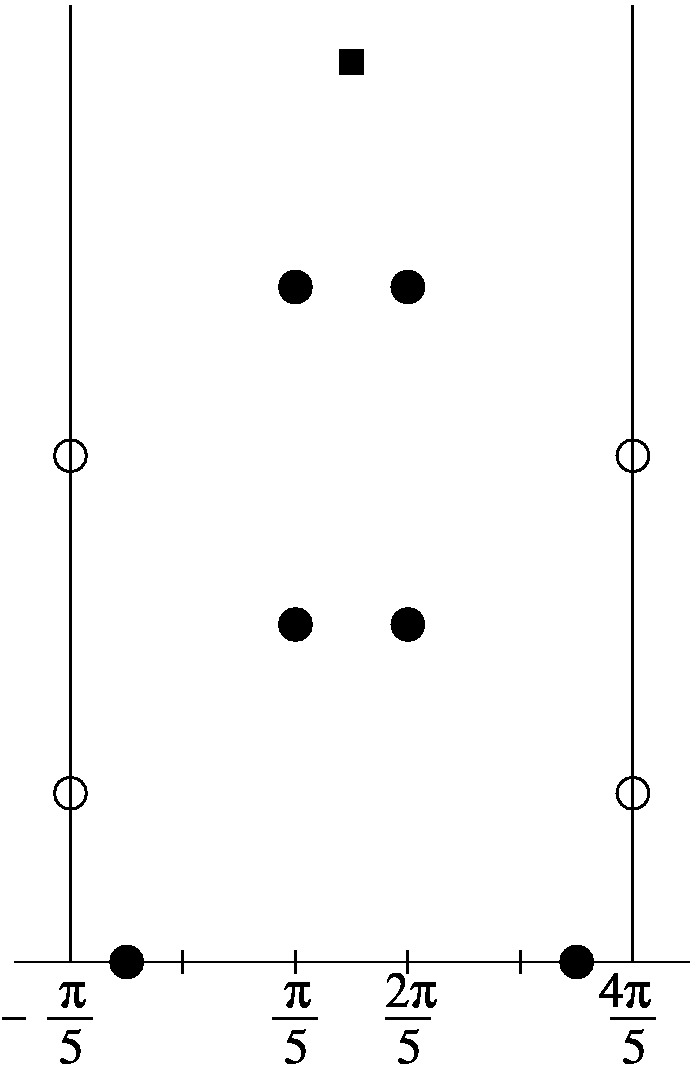
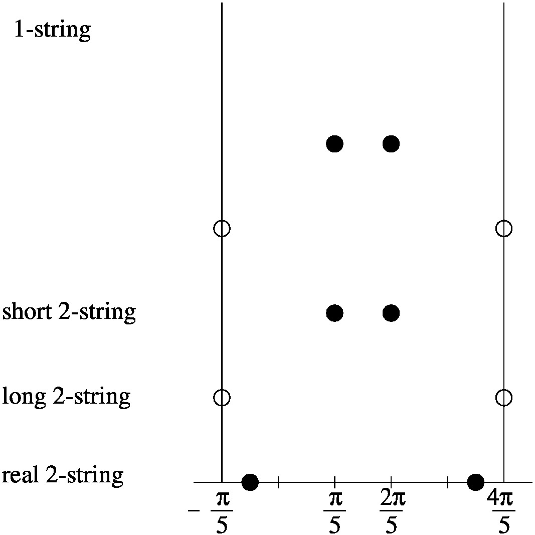
Figure 4.1: Typical configuration of zeros of the transfer matrix eigenvalue. The boundary condition $(1,1)$ is on the left, while $(1,2)$ is on the right.

The $1$-string $u_{j}=3\pi/10+iv_{j}$ lies in the middle of the analytical strip and has real part $3\pi/10$ and exist in the $(1,1)$ sector only. The two zeros of a short $2$-string $u_{j}=\pi/5+iw_{j}$, $2\pi/5+iw_{j}$ have common imaginary parts and real parts $\pi/5$, $2\pi/5$ respectively. The two zeros of a long $2$-string $u_{j}=-\pi/5+iw_{j}$, $4\pi/5+iw_{j}$ have common imaginary parts and real parts $-\pi/5$, $4\pi/5$ respectively so that these zeros sit at the edge of the analytical strip. Lastly, a real 2-string consists of a pair of zeros $u_{j}=\pi/10,\pi/2$ on the real axis. The string contents satisfy the $(m,n)$ system

$$2m+n+3-s=N\Leftrightarrow m+n=N-3+s,\qquad s=1,2$$ (4.34)

$$m=\text{\{number of short $2$-strings\}},\qquad n=\text{\{number of long $2$-strings\}}$$ (4.35)

There is always a real 2-string on the real axis and, in the $(r,s)=(1,1)$ sector, a single $1$-string furthest from the real axis. Each “short $2$-string" contributes two zeros and, by periodicity, each “long $2$-string contributes one zero. The 1-string contributes one zero and so does the real 2-string since it is shared between the upper and lower half planes. Consequently, the $(m,n)$ system expresses the conservation of the total number of zeros in a periodicity strip. The roles of $m$ and $n$ are interchanged under duality. For the leading excitations $m$ is finite but $n\sim N$ as $N\to\infty$.

As explained in [47], an excitation with string content $(m,n)$ is uniquely labeled by a set of quantum numbers

$$I=(I_{1},I_{2},\ldots,I_{m})$$ (4.36)

where the integers $I_{j}\geq 0$ give the number of long 2-strings whose imaginary parts $w_{j}$ are greater than that of the given short 2-string $v_{j}$. The short 2-strings $v_{j}$ and long 2-strings $w_{j}$ labeled by $j=1$ are closest to the real axis. The quantum numbers $I_{j}$ satisfy

$$n\geq I_{1}\geq I_{2}\geq\dots\geq I_{m}\geq 0.$$ (4.37)

For given string content $(m,n)$, the lowest excitation occurs when all of the short 2-strings are further out from the real axis than all of the long 2-strings. In this case all of the quantum numbers vanish $I_{j}=0$. Bringing the location of a short 2-string closer to the real axis by interchanging the location of the short 2-string with a long 2-string increments its quantum number by one unit and increases the energy.

Finitized characters

For $N=s-1$ (mod 2), the (fermionic) finitized characters are

$$(r,s)=(1,1): \chi_{0}^{(N)}(q)=\sum_{m=0}^{(N-2)/2}q^{m^{2}+m}\left[\begin{array}[]{c}N-2-m\\ m\end{array}\right]_{q}\to\chi_{0}(q)$$ (4.40)

$$(r,s)=(1,2): \chi_{-1/5}^{(N)}=\sum_{m=0}^{(N-1)/2}q^{m^{2}}\left[\begin{array}[]{c}N-1-m\\ m\end{array}\right]_{q}\to\chi_{1}(q)$$ (4.43)

where

$$\left[\begin{array}[]{c}N\\ m\end{array}\right]_{q}=\prod_{i=1}^{m}\frac{1-q^{N+1-i}}{1-q^{i}}\to\prod_{i=1}^{m}\frac{1}{1-q^{i}}\quad\mbox{for}\quad N\to\infty$$

These finitized characters can also be written in the form

$$\chi_{1,s}^{(N)}(q)=\sum q^{E}=\sum_{\sigma}q^{\sum_{j=1}^{N-1}jH(\sigma_{j-1},\sigma_{j},\sigma_{j+1})}$$ (4.44)

where the sum is over all one-dimensional RSOS paths $\sigma=\{\sigma_{0},\sigma_{1},\ldots,\sigma_{N}\}$ on $A_{4}$ with $\sigma_{0}=s$ and $\sigma_{N}=1$. The energy function $H$ is

$$H(\sigma_{j-1},\sigma_{j},\sigma_{j+1})=\begin{cases}1,&(\sigma_{j-1},\sigma_{j},\sigma_{j+1})=(2,1,2)\ \mbox{or}\ (3,4,3)\\ 0,&\text{otherwise}\end{cases}$$ (4.45)

Notice that this local energy function differs from the one introduced by Forrester and Baxter.

Bijection between RSOS paths, strings and Virasoro modes

There is in fact a bijection [50] between the one-dimensional RSOS paths $\sigma$ that label the eigenstates (eigenvalues), the allowed patterns of strings in the periodicity strip and the state described in terms of the Virasoro modes. A triple $(\sigma_{j-1},\sigma_{j},\sigma_{j+1})=(2,1,2)$ or $(3,4,3)$ corresponds to a short $2$-string (particle) at position $j$ and an insertion of a Virasoro mode $L_{-j}$ whereas a pair segment $(\sigma_{j},\sigma_{j+1})=(2,3)$ or $(3,2)$ corresponds to a long $2$-string (dual particle) at position $j+\frac{1}{2}$. In addition, in the sector $(r,s)=(1,1)$, there is a $1$-string at $j=0$ corresponding to the initial height $s=1$ at $j=0$. This bijection is illustrated in Figure 4.2. Notice that only the relative positions of the long and short $2$-strings is important. If $s=1$ the first and last ($3-s$) segments are inactive whereas, if $s=2$, only the last ($3-s$) segments are inactive. We see that the geometric constraint

$$2m+n+3-s=N$$ (4.46)

agrees with the $(m,n)$ system.

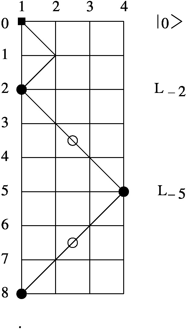
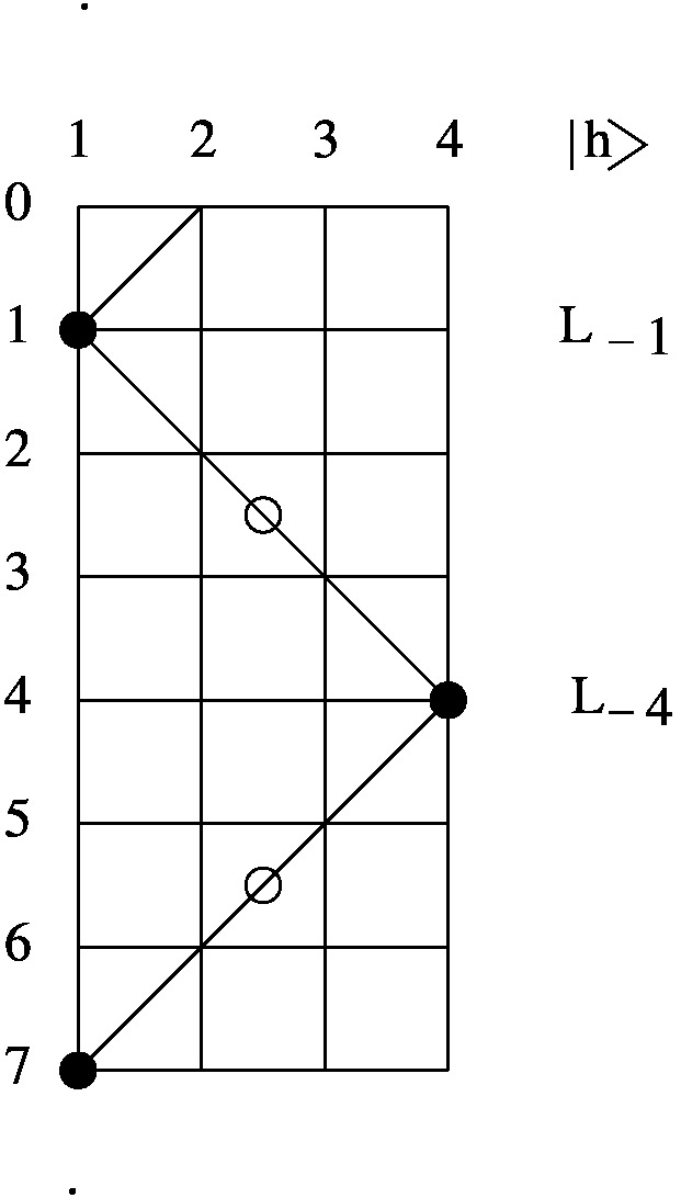
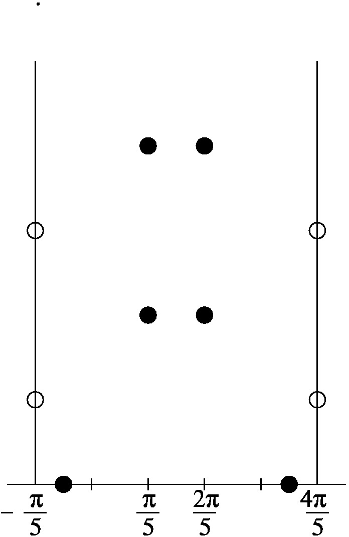
Figure 4.2: Bijection of one-dimensional configurational paths $\sigma$, strings in the periodicity strip for the $(r,s)=(1,1)$ sector and the Virasoro modes over $|0\rangle$ is shown on the left part. The right part contains the analogous figures for the case $(r,s)=(1,2)$. The paths $\sigma$ (rotated $90^{\circ}$ clockwise) are shown on the left and the analytical strip containing a $1$-string (solid square), short 2-strings (solid circles) and $2$-strings (open circles) in the upper-half complex $u$-plane are shown on the right. For each short two strings we associate a Virasoro mode where they are located, $L_{-2}$ and $L_{-5}$ in the ($1,1$) and $L_{-1}$ , $L_{-4}$ in the $(1,2)$ cases. The string (particle) content is $m=n=2$ with $N=8$ in the $(1,1)$ and with $N=7$ in the $(1,2)$ cases. The energies of these excited states are $E=2+5=7$ ($E=1+4=5)$ since there are two particles (short $2$-strings) at respective positions $j=2,5$ ($1,4)$, respectively. The corresponding states in the Virasoro modules are $L_{-5}L_{-2}|0\rangle$ and $L_{-4}L_{-1}|h\rangle$.

Flow between boundary conditions

We are in the position now to describe the boundary flows induced by $\xi$ between the boundary conditions $(1,1)$ and $(1,2)$. This flow is realized when $\xi$ goes from $0$ to $\infty$ and we can describe it at the three different languages we already introduced.

In terms of the zeros and $(n,m)$ system the flow is very simple: the 1-string which exist only for the $(1,1)$ boundary condition start to move to infinity in the imaginary direction as indicated on the figure. There is no change in the 2-strings.

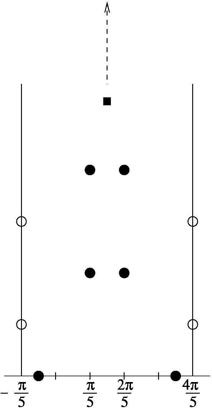
Figure 4.3: The boundary flow in terms of the zeros. On the left $\xi=0$ while on the right $\xi=\infty$. In the $\xi\to\infty$ limit, shown in the middle, nothing else happens than the imaginary location of the 1-string moves to infinity and disappears. The distribution of the 2-strings are not affected at all.

The flow in terms of the paths is also simple we merely have to remove the first raw of the pathspace.

Most enlightening is the flow in terms of the Virasoro modes. First of all the highest weight state $|0\rangle$ flows to $|\Phi\rangle$, and in the module the rule is very simple we have to increase the index of every Virasoro mode by one $L_{-n}\to L_{-n+1}$:

$$L_{-n_{1}}L_{-n_{2}}...L_{-n_{k}}|0\rangle\rightarrow L_{-n_{1}+1}L_{-n_{2}+1}...L_{-n_{k}+1}|h\rangle$$

This very simple flow is summarized for the first few excited states in the following table

Level	State in the $(1,1)$ module	State in the $(1,2)$ module	Level
h.w. state	$|0\rangle$	|$\Phi\rangle$	h.w. state
2	$L_{-2}|0\rangle$	$L_{-1}|\Phi\rangle$	1
3	$L_{-3}|0\rangle$	$L_{-2}|\Phi\rangle$	2
4	$L_{-4}|0\rangle$	$L_{-3}|\Phi\rangle$	3
5	$L_{-5}|0\rangle$	$L_{-4}|\Phi\rangle$	4
6	$L_{-2}L_{-4}|0\rangle$	$L_{-1}L_{-3}|\Phi\rangle$	4
6	$L_{-6}|0\rangle$	$L_{-5}|\Phi\rangle$	5
7	$L_{-2}L_{-5}|0\rangle$	$L_{-1}L_{-4}|\Phi\rangle$	5
7	$L_{-7}|0\rangle$	$L_{-6}|\Phi\rangle$	6
8	$L_{-2}L_{-6}|0\rangle$	$L_{-1}L_{-5}|\Phi\rangle$	6
8	$L_{-3}L_{-5}|0\rangle$	$L_{-2}L_{-4}|\Phi\rangle$	6
8	$L_{-8}|0\rangle$	$L_{-7}|\Phi\rangle$	7
9	$L_{-2}L_{-7}|0\rangle$	$L_{-1}L_{-6}|\Phi\rangle$	7
9	$L_{-3}L_{-6}|0\rangle$	$L_{-2}L_{-5}|\Phi\rangle$	7
9	$L_{-9}|0\rangle$	$L_{-8}|\Phi\rangle$	8

As expected and shown in the table above, the character will flow from $X_{1,1}=1+q^{2}+q^{3}+q^{4}+q^{5}+2q^{6}+2q^{7}+3q^{8}+3q^{9}+...$ to $X_{1,2}=1+q+q^{2}+q^{3}+2q^{4}+2q^{5}+3q^{6}+3q^{7}+...$.

The level by level flow agrees with the TCSA result of [90]

4.2.1.2 Periodic case

The best way to describe the periodic case is based on the previously introduced boundary identification. In analyzing the zeros of the transfer matrix we can distinguish two different appearance of zeros as shown on the figure 4.4

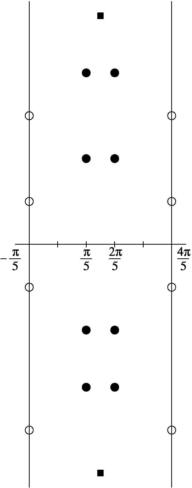
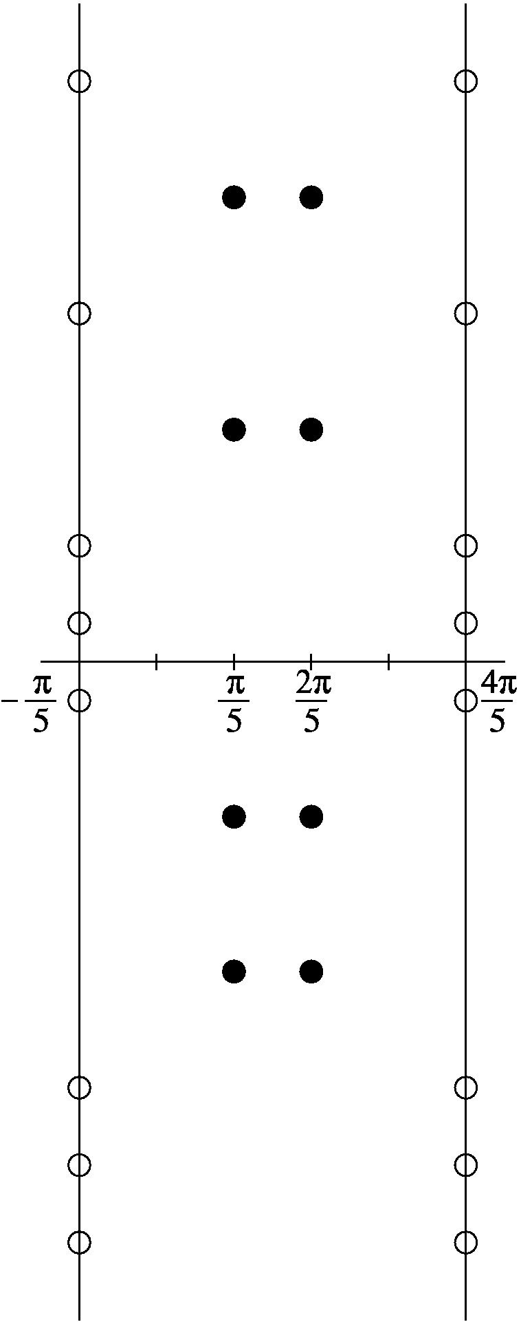
Figure 4.4: The two appearing configurations of zeros of the transfer matrix eigenvalue in the periodical case.

The first we can recognize is that we have similar short and long 2-strings and 1-strings as in the boundary case. What is different, however, is that the zeros on the lower half plane are not necessarily related to those on the upper half plane except for the 1-string. So if we have a 1-string on the lower half we always have one the upper half, too. In classifying the states we can use the already developed classification for the boundary case, taking into account that the lower and upper halves are independent.

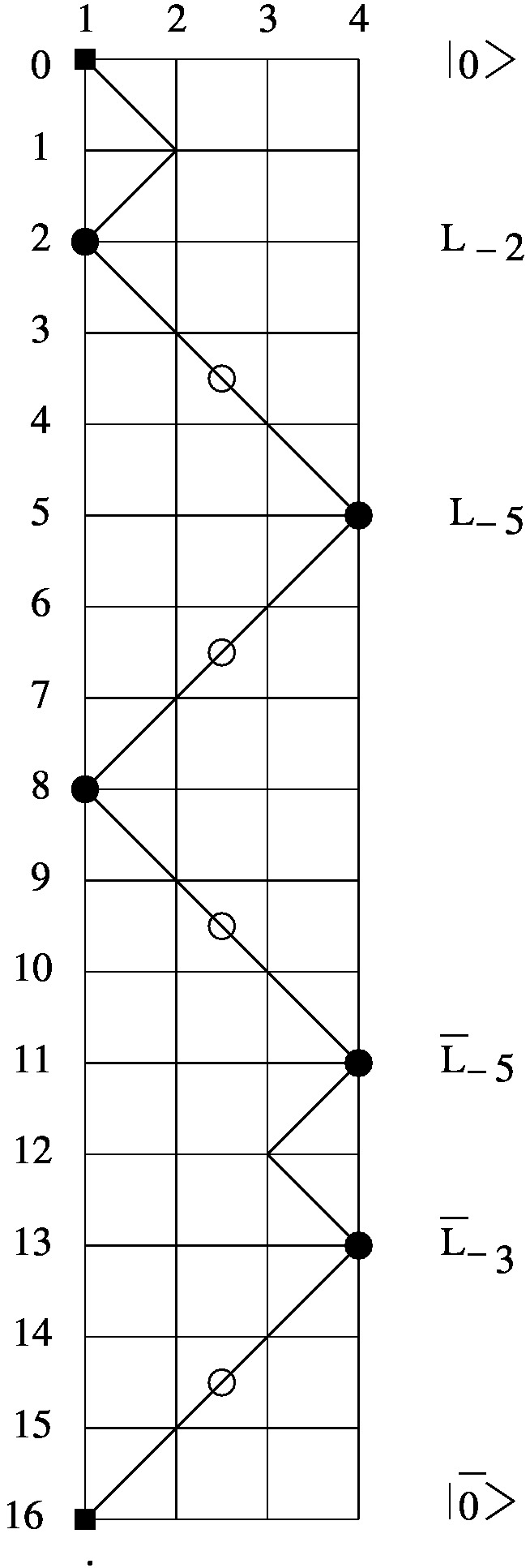
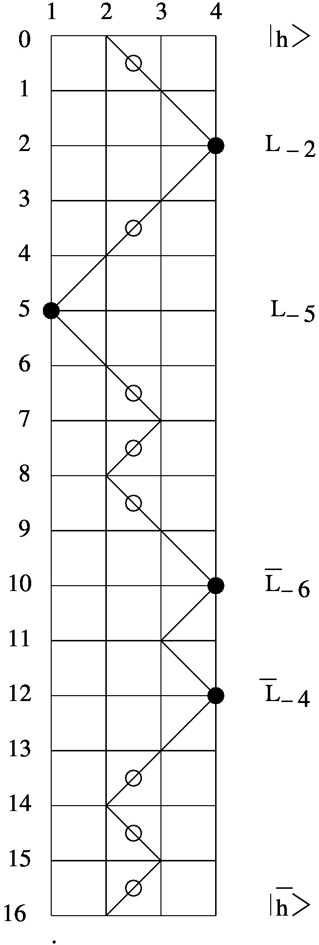
Figure 4.5: The identification between the zeros of the transfer matrix, paths and Virasoro modes in the periodical case.

For the $(m,n)$ structure, we have to differentiate between the structures on the 2 sides of the real axis. Now our lattice is $2N$ dimensional with $N$ zeroes on each side. We define an $(m,n;\bar{m},\bar{n})$ system. On each side the eigenvalues with zeros at $\frac{3\pi}{10}$ correspond to the $s=1$ and have $N-2$ zeros, while the other eigenvalues lie in the $s=2$ sector with $N$ zeros. Formulating this, we get that $2m+n-2s+4=N$ or equivalently $2m+n=N+2s-4$, where $m$ is the number of the short 2-strings and $n$ is the number of long 2-strings. Similarly $2\bar{m}+\bar{n}=N+2s-4$.

Studying the zero structures, we find that they resemble the Hilbert spaces of $\bar{V_{1}}\otimes V_{1}$ for the structures with zeroes with the 1-string and $\bar{V_{2}}\otimes V_{2}$ for those without the 1-string. In fact, the real axis separates the $\bar{V_{1}}$ and $\bar{V_{2}}$ parts of the tensored states from the $V_{1}$ and $V_{2}$ respectively. We define the vacuum $|0\rangle$ as the state with $|0,0\rangle$ and the (1,2) ground state $|\Phi\rangle$ as the $|\frac{-1}{5},\frac{-1}{5}\rangle$ state.

The state with one short string furthest from the real axis up below the 1 string corresponds to $L_{-2}|0\rangle$ and moving the short string downwards through the long strings increases the level by 1 for each permutation, thus creating the $L_{-n}|0\rangle$ states. The mirror image on the zeroes below the real axis corresponds to the $\bar{L}_{-n}|0\rangle$. A similar description also applies for $L_{-n_{1}}...L_{-n_{N}}|0\rangle$.

For the (1,2) states, the lowest excitation appears with a short string on the top of all long strings, with no 1-string above. This is $L_{-1}|\Phi\rangle$, and every time we lower the short string below a long string we obtain one extra unit of energy, hence we have all the $L_{-n}|\Phi\rangle$ and similarly for the mirror image of $\bar{L}$ and for combinations of those.

Summarizing, in this model we find out that the first few states that we obtain from the classification of the zeros of the eigenvalues are:

Level	$\bar{V_{1}}\otimes V_{1}$	$\bar{V_{2}}\otimes V_{2}$
0	$|0\rangle$	$|\Phi\rangle$
1		$L_{-1}|\Phi\rangle$, $\bar{L}_{-1}|\Phi\rangle$
2	$L_{-2}|0\rangle$, $\bar{L}_{-2}|0\rangle$	$L_{-2}|\Phi\rangle$, $\bar{L}_{-2}|\Phi\rangle$, $\bar{L}_{-1}L_{-1}|\Phi\rangle$
3	$L_{-3}|0\rangle$ , $\bar{L}_{-3}|0\rangle$	$L_{-3}|\Phi\rangle$, $\bar{L}_{-3}|\Phi\rangle$, $\bar{L}_{-2}L_{-1}|\Phi\rangle$, $\bar{L}_{-1}L_{-2}|\Phi\rangle$
4	$L_{-4}|0\rangle$ , $\bar{L}_{-4}|0\rangle$, $\bar{L}_{-2}L_{-2}|0\rangle$	$L_{-4}|\Phi\rangle$, $L_{-3}L_{-1}|\Phi\rangle$, $L_{-3}\bar{L}_{-1}|\Phi\rangle$, $L_{-2}\bar{L}_{-2}|\Phi\rangle$,
		$\bar{L}_{-3}L_{-1}|\Phi\rangle$, $\bar{L}_{-3}\bar{L}_{-1}|\Phi\rangle$, and $\bar{L}_{-4}|\Phi\rangle$

Table 2 lists the first few states that we can see from the zero eigenvalues of the periodic transfer matrix. In a lattice of $2N$ sites, one can read all the states up to level $N$ completely. The same can be done from the RSOS paths in the Hilbert space.

4.2.1.3 The case of a seam

Introducing a seam we can analyze the two limiting cases similarly we analyzed in the boundary setting, namely $\xi$ going from $0$ to $\infty$. Clearly for $\xi=0$ the seam disappears (identity seam) and we recover the results of the periodic boundary condition. In the $\xi\to\infty$ limit we found the following identification between the strings the paths and the Virasoro modes

-

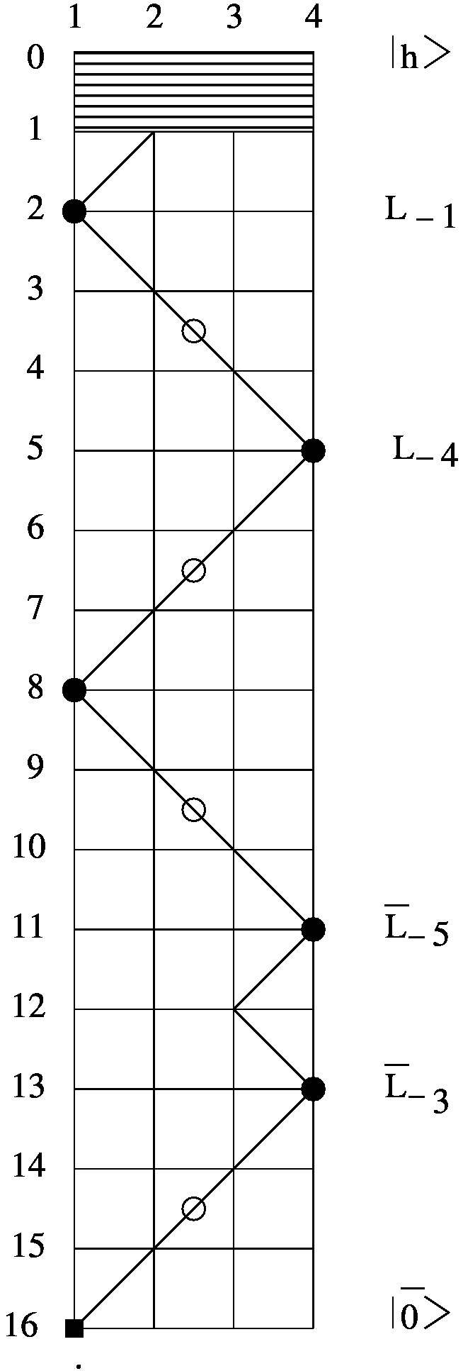
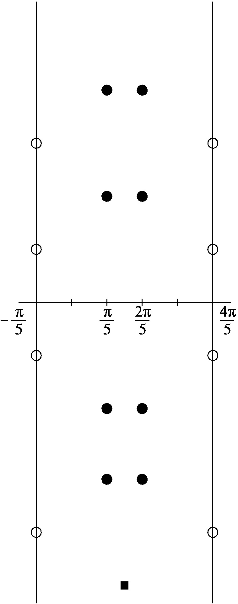
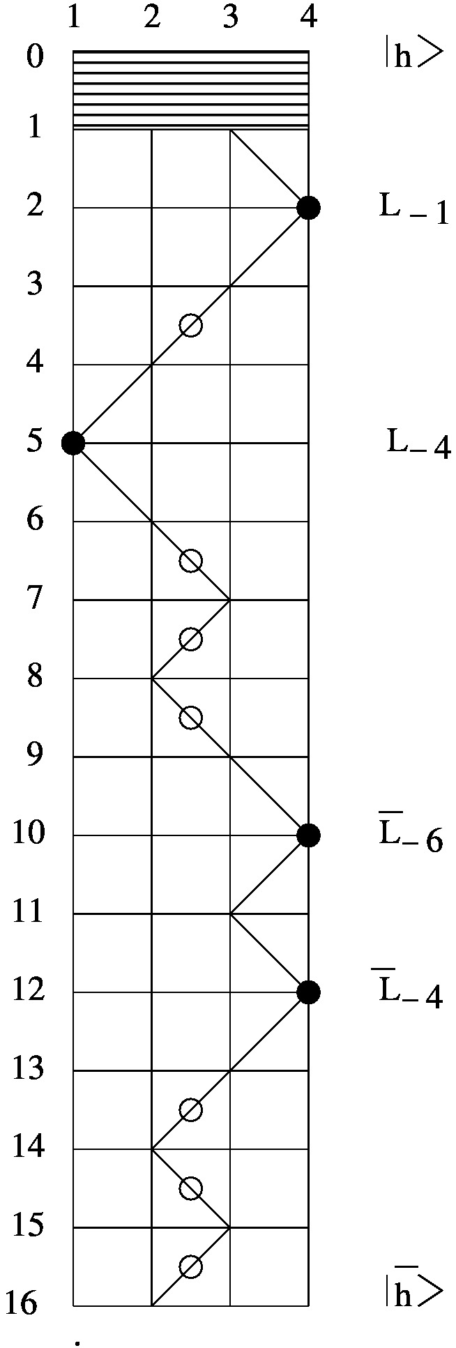
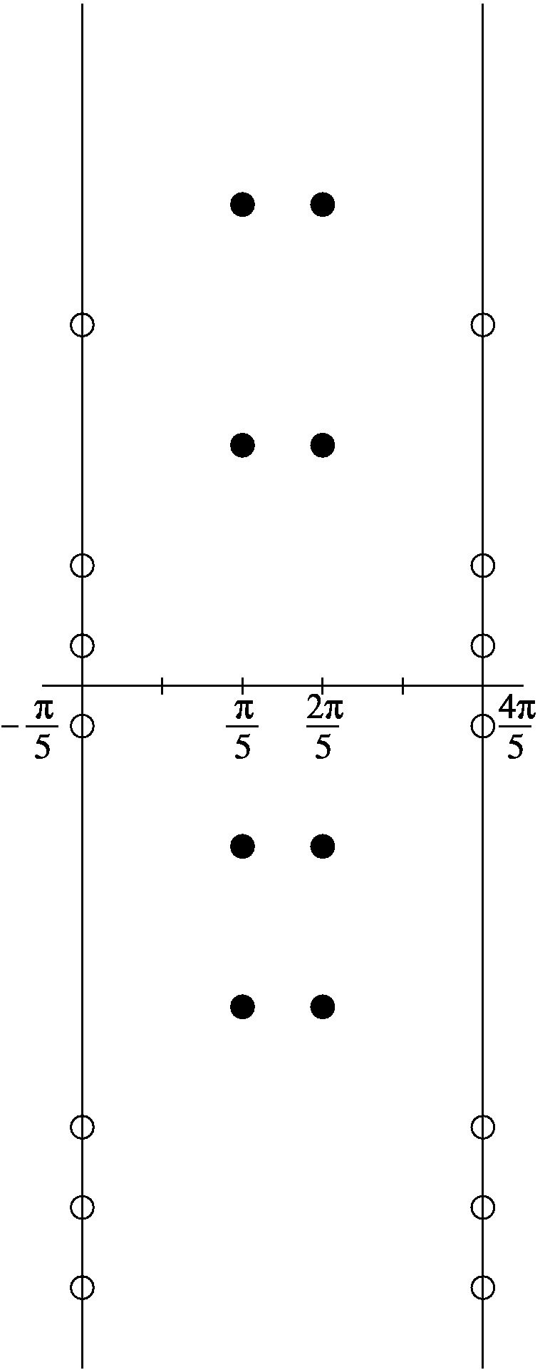
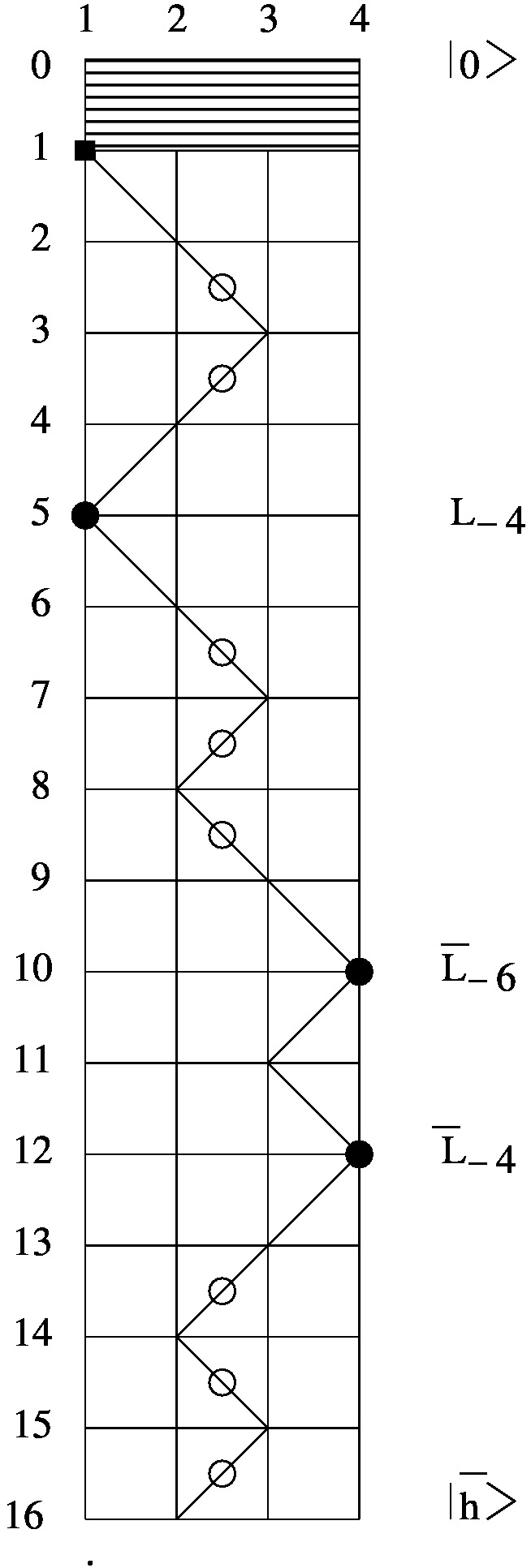
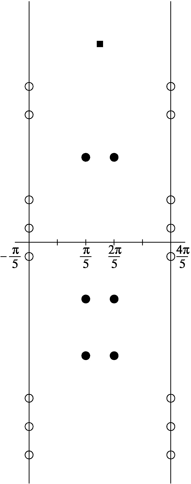
Figure 4.6: The identification between the zeros of the transfer matrix, paths and Virasoro modes in the case of a seam at the first site. The seam shadows the periodicity of the paths.

The flows are very simple in terms of the zeros. We have the following simple mechanism. The flows can be explained in three mechanisms:

A. If the outermost string is a 1-string, it flows towards infinity with increasing $b$. (Plot on the left)

B. If the outermost string is a short 2-string, one of the zeroes flows to infinity and the other goes to $\frac{3\pi}{10}$. (Plot on the right)

C. If the outermost string is a long 2-string, it flows towards infinity. (Plot in the middle)

In terms of the states this is summarized as follows:

1. Due to type A flows:

$$L_{-N_{1}}...L_{-N_{n}}\bar{L}_{-\bar{N}_{1}}....\bar{L}_{-\bar{N}_{n}}|0\rangle\rightarrow L_{-N_{1}}...L_{-N_{n}}\bar{L}_{-\bar{N}_{1}+1}....\bar{L}_{-\bar{N}_{n}+1}|\bar{\phi}\rangle$$

with $|0\rangle\rightarrow|\bar{\phi}\rangle$

2. Due to type B flows:

$$(L_{-N_{1}}...L_{-N_{n}}\bar{L}_{-\bar{N}_{1}}....\bar{L}_{-\bar{N}_{n}})\bar{L}_{-1}|\Phi\rangle\rightarrow(L_{-N_{1}}...L_{-N_{n}}\bar{L}_{-\bar{N}_{1}+1}....\bar{L}_{-\bar{N}_{n}+1})|\phi\rangle$$

3. Due to type C flows:

$$L_{-N_{1}}...L_{-N_{n}}\bar{L}_{-\bar{N}_{1}}....\bar{L}_{-\bar{N}_{n}}|\Phi\rangle\rightarrow L_{-N_{1}}...L_{-N_{n}}\bar{L}_{-\bar{N}_{1}+1}....\bar{L}_{-\bar{N}_{n}+1}|\Phi\rangle$$

Now using the first few states of the trivial defect case from Table 2, we will deduce their corresponding states using this mechanism, and it is indeed what we can observe from the flows of the zero eigenvalues as was shown for sample states above.

Level	Trivial Defect	Non-trivial Defect	Level
h.w. state	$|0\rangle$	|$\bar{\phi}\rangle$	h.w. state
h.w. state	|$\Phi\rangle$	|$\Phi\rangle$	h.w. state
1	$\bar{L}_{-1}|\Phi\rangle$	$|\phi\rangle$	h.w. state
1	$L_{-1}|\Phi\rangle$	$L_{-1}|\Phi\rangle$	1
2	$\bar{L}_{-2}|0\rangle$	$\bar{L}_{-1}$$|\bar{\phi}\rangle$	1
2	$\bar{L}_{-2}|\Phi\rangle$	$\bar{L}_{-1}|\Phi\rangle$	1
2	$\bar{L}_{-1}L_{-1}|\Phi\rangle$	$L_{-1}|\phi\rangle$	1
2	$L_{-2}|\Phi\rangle$	$L_{-2}|\Phi\rangle$	2
2	$L_{-2}|0\rangle$	$L_{-2}|\bar{\phi}\rangle$	2
3	$\bar{L}_{-3}|0\rangle$	$\bar{L}_{-2}$$|\bar{\phi}\rangle$	2
3	$\bar{L}_{-3}|\Phi\rangle$	$\bar{L}_{-2}|\Phi\rangle$	2
3	$\bar{L}_{-2}L_{-1}|\Phi\rangle$	$\bar{L}_{-1}L_{-1}|\Phi\rangle$	2
3	$\bar{L}_{-1}L_{-2}|\Phi\rangle$	$L_{-2}|\phi\rangle$	2
3	$L_{-3}|\Phi\rangle$	$L_{-3}|\Phi\rangle$	3
3	$L_{-3}|0\rangle$	$L_{-3}|0\rangle$	3
4	$\bar{L}_{-1}\bar{L}_{-3}|\Phi\rangle$	$\bar{L}_{-2}|\phi\rangle$	2

Table 3 shows the exact flow from each state in the trivial defect Hilbert Space to its corresponding state in the non-trivial one up to the second order descendent level in the defect Hilbert space.

It can be seen that the flow occurs from $\bar{V}_{1}\otimes V_{1}+\bar{V}_{2}\otimes V_{2}$ to $\bar{V}_{1}\otimes V_{2}+\bar{V}_{2}\otimes V_{1}+\bar{V}_{2}\otimes V_{2}$ as we expect from defect conformal field theory. Had we taken the limit $b\rightarrow-\infty$, we would have got the similar total outcome, but with $\phi$ and $\bar{\phi}$ exchanged, and $L_{-n}$ being the operator augmented to $L_{-n+1}$ instead of $\bar{L}$ as happens here.

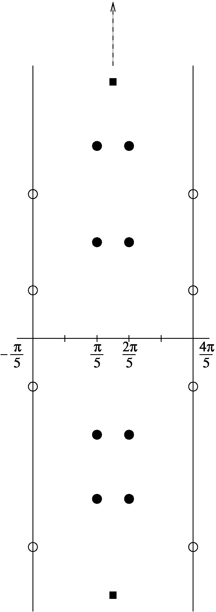
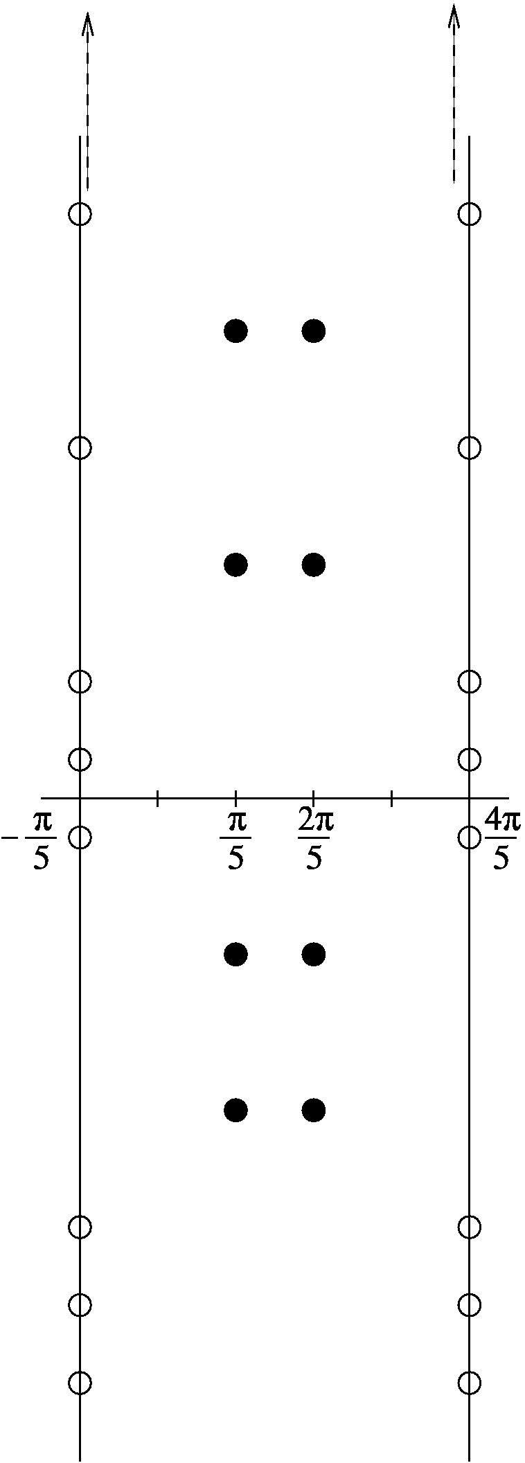
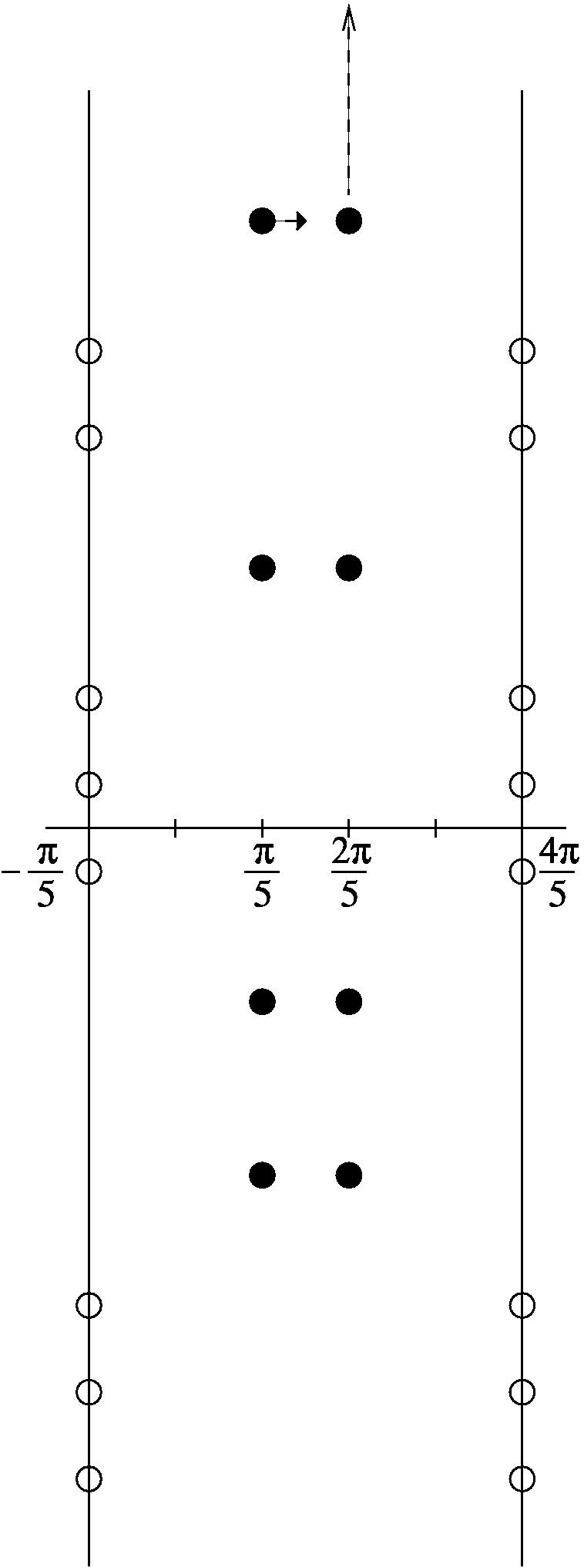
Figure 4.7: The identification between the zeros of the transfer matrix, paths and Virasoro modes in the case of a seam at the first site. The seam shadows the periodicity of the paths. The two figures on the left correspond to type A flow, the outermost 1-string flows to infinity, and the state flows from $L_{-3}L_{-5}\bar{L}_{-2}\bar{L}_{-5}|0\rangle\rightarrow L_{-3}L_{-5}\bar{L}_{-1}\bar{L}_{-4}|\bar{\phi}\rangle$. The middle two figures are of type C, the long 2-string goes away to infinity and the state flows from $L_{-4}L_{-6}\bar{L}_{-2}\bar{L}_{-5}|\Phi\rangle\rightarrow L_{-4}L_{-6}\bar{L}_{-1}\bar{L}_{-4}|\Phi\rangle$. Finally the two figures on the right show how a short 2-string has one of its zeroes flow to infinity and the other to the middle $u=\frac{3\pi}{10}$, and the state flows from $L_{-4}L_{-6}\bar{L}_{-1}\bar{L}_{-5}|\Phi\rangle\rightarrow L_{-4}L_{-6}\bar{L}_{-4}|\phi\rangle$

4.3 TBA Equations

In this section we solve the TBA equations of the Lee-Yang model for the periodic boundary conditions with and without a seam, and for the boundary model in both the critical and the massive cases. We derive those equations on the lattice, and after scaling we confirm the results of the continuum limit equations which were derived in [91, 37, 90]. Our approach is systematic since we know the analytic structure and the zero eigenvalue locations in the analytic strip, which allows us to solve the TBAs taking into account this structure.

4.3.1 Critical/Massless TBAs:

4.3.1.1 Periodic boundary conditions

The transfer matrix satisfies the functional relation

$$T(u)T(u+\lambda)=\left(\frac{\sin(\lambda+u)\sin(\lambda-u)}{\sin^{2}\lambda}\right)^{N}+\left(\frac{\sin u}{\sin\lambda}\right)^{N}T(u+3\lambda)$$

We normalize the transfer matrix as:

$$t(u)=\left(\frac{s(\lambda)s(u+2\lambda)}{s(u+\lambda)s(u+3\lambda)}\right)^{N}T_{1}(u)$$

and we get that

$$t(u)t(u+\lambda)=1+t(u+3\lambda)$$

Using the periodicity $t(u)=t(u+\pi)$ we rewrite it as $t(u)t(u-\frac{2\pi}{5})=1+t(u-\frac{\pi}{5})$, and after shifting $u$ we have

$$t(u+\frac{\pi}{5})t(u-\frac{\pi}{5})=1+t(u)$$

We decompose $t$ into two components $f$ and $l$:

$$t(u)=f^{N}(u)l(u)$$

where $f^{N}$ corresponds to the bulk free energy (order $N$ term) and $l$ corresponds to the finite size corrections (order $\frac{1}{N}$ term) and $N$ is even. We want to kill the $N$th order zeros at $-\frac{\pi}{5},\frac{4\pi}{5}$ and poles at $\frac{\pi}{5},\frac{2\pi}{5}$ in $f(u)$ which satisfies

$$f(u+\frac{\pi}{5})f(u-\frac{\pi}{5})=f(u)$$

The solution compatible with the analytical structure is

$$f(u)=\frac{\sin\frac{5u}{3}+\sin\frac{\pi}{3}}{\sin\frac{5u}{3}-\sin\frac{\pi}{3}}=-\tan(\frac{5u}{6}+\frac{\pi}{6})\tan(\frac{5u}{6}+2\frac{\pi}{6})$$

which is basically the shifted S-matrix. $f(u)$ satisfies $f(u)f(u+\lambda)=1$. Introducing the variable $\ u=\frac{3\pi}{10}+\frac{3ix}{5}\$ we write the functional equation as

$$t(x-i\frac{\pi}{3})t(x+i\frac{\pi}{3})=1+t(x)$$

In this variable

$$f(x)=-\tan(\frac{ix}{2}+\frac{5\pi}{12})\tan(\frac{ix}{2}+\frac{7\pi}{12})$$ (4.47)

Vacuum state:

The ground state has no zeroes inside the analytical strip, and since it is analytic in the strip, we can use the functional relation to write

$$\frac{t(x-i\frac{\pi}{3})t(x+i\frac{\pi}{3})}{t(x)}=\frac{l(x-i\frac{\pi}{3})l(x+i\frac{\pi}{3})}{l(x)}=1+t^{-1}(x)$$

For the ground state, inside the physical strip $x\in[-\frac{i\pi}{3},\frac{i\pi}{3}]$, both sides of the equation are ANZ, so we can take the log and solve in Fourier space, then

$$\log l(x)=-\varphi\star\log(1+t^{-1}(x))\qquad;\qquad\hat{\varphi}=\frac{1}{1-e^{k\frac{\pi}{3}}-e^{-k\frac{\pi}{3}}}$$

where

$$\ \varphi(x)=\frac{1}{2\pi}\underset{-\infty}{\overset{\infty}{\int}}dk\hat{\varphi}e^{ikx}\$$

and

$$\ \varphi\star f=\underset{-\infty}{\overset{\infty}{\int}}dy\varphi(x-y)f(y)$$ (4.48)

Now we restore $t$:

$$\log t(x)=N\log f(x)-\varphi\star\log(1+t^{-1}(x))$$ (4.49)

This is the ground-state TBA on the lattice. In the thermodynamic limit all interesting things happen around two domains: in the $u$ variable either on the upper half plane around $\frac{3}{5}i\log N$ or on the lower half plane around $-\frac{3}{5}i\log N$. For this reason in the $x$ variable we focus on the behavior around $\pm\log N$. Let us center the new functions around $x\pm\log N$ as $e^{\epsilon^{\pm}(x)}=\underset{N\to\infty}{\lim}t(x\pm\log N)$. Taking the continuum limit ($N\to\infty$) on the source term we get

$$N\lim_{N\to\infty}\log f(x+\log N)=N\lim_{N\to\infty}\log(1+4\sin\frac{\pi}{3}e^{\mp x}\frac{1}{N}+\dots)=4\sin\frac{\pi}{3}e^{\mp x}$$

which leads to the massless ground-state TBA equations

$$\epsilon^{\pm}(x)=4\sin\frac{\pi}{3}e^{\mp x}-\varphi\star\log(1+e^{-\epsilon^{\pm}(x)})$$ (4.50)

where $4\sin\frac{\pi}{3}$ can be easily absorbed by shifting $x$.

Excited states:

From our numerics, we know that in the excited states there are zero eigenvalues in the analycity strip. We classified them before as 1-strings and short 2-strings. The 1-strings occur at

$$u=\frac{3\pi}{10}+i\alpha$$

and additionally the short strings at

$$u=\begin{cases}\frac{\pi}{5}+i\beta_{j}\\ \frac{2\pi}{5}+i\beta_{j}\end{cases}$$

For finite energy states in the continuum ($N\to\infty$) limit, they go to infinity as $\alpha=\frac{3}{5}(\pm\log N+\tilde{\alpha}^{\pm})$ and $\beta_{j}=\frac{3}{5}(\pm\log N+\tilde{\beta}_{j}^{\pm})$ on the upper/lower half plane, respectively as it can be analyzed numerically.

In the $x=\frac{5}{3i}(u-\frac{3\pi}{10})$ variable they are located at

$$\begin{array}[]{cc}x_{0}^{\pm}=\frac{5\alpha}{3}=\log N+\tilde{\alpha}^{\pm}\\ x_{j}^{\pm}=\pm i\frac{\pi}{6}+\log N+\tilde{\beta}_{j}^{\pm}\end{array}$$

As we would like to take logarithm we need functions free of zeros and poles on the physical strip. The function which can eliminate the single zero is

$$\sigma_{0}(x)=\tanh\left(\frac{3}{4}x\right)$$ (4.51)

while the one which eliminates the two zeros at $\pm\frac{\pi}{6}$ is

$$\sigma_{1}(x)=f(x)^{-1}=\frac{\cosh x+\sin\frac{\pi}{3}}{\cosh x-\sin\frac{\pi}{3}}$$ (4.52)

These functions satisfy

$$\begin{array}[]{cc}\sigma_{0}(x-\frac{i\pi}{3})\sigma_{0}(x+\frac{i\pi}{3})=1\\ \sigma_{1}(x-\frac{i\pi}{3})\sigma_{1}(x+\frac{i\pi}{3})=\sigma_{1}(x)\end{array}$$ (4.53)

With these functions we parametrize the normalized transfer matrix eigenvalue as

$$t(x)=f(x)^{N}\prod_{\pm}\sigma_{0}(x-x_{0}^{\pm})\prod_{j=1}^{M}\sigma_{1}(x-x_{j}^{\pm})l(x)$$ (4.54)

which ensures that $l(x)$ is ANZ in the physical strip. The functional equation then takes the form

$$\prod_{\pm}\sigma_{0}(x-x_{0}^{\pm})\frac{t(x-i\frac{\pi}{3})t(x+i\frac{\pi}{3})}{t(x)}=\frac{l(x-i\frac{\pi}{3})l(x+i\frac{\pi}{3})}{l(x)}=\prod_{\pm}\sigma_{0}(x-x_{0}^{\pm})(1+t^{-1}(x))$$ (4.55)

Clearly both sides are ANZ in the interior of the physical strip: the combination $\prod_{\pm}\sigma_{0}(x-x_{0}^{\pm})t^{-1}(x)$ is regular at $x=x_{0}^{\pm}.$ Taking then logarithm and going to Fourier space we find:

$$\log l(x)=-\varphi\star\log(\prod_{\pm}\sigma_{0}(x-x_{0}^{\pm})(1+t^{-1}(x)))$$

Restoring $t$ we obtain the excited-state massless TBA equation on the lattice:

$$\begin{array}[]{cc}\log t(x)=N\log f(x)+\sum_{\pm}\log(\sigma_{0}(x-x_{0}^{\pm}))+\sum_{j,\pm}\log(\sigma_{1}(x-x_{j}^{\pm}))\\ -\varphi\star\log(\prod_{\pm}\sigma_{0}(x-x_{0}^{\pm})(1+t^{-1}(x)))\end{array}$$ (4.56)

The parameters of the excited state $x_{i}=\{x_{0}^{\pm},x_{j}^{\pm}\}$ are determined self-consistently from the fact that it is a zero of the transfer matrix:

$$t(x)|_{x=x_{i}\pm\frac{i\pi}{3}}=-1$$

In the scaling limit we can focus on the two scaling domains at $\pm\log N$ by introducing

$$e^{\epsilon^{\pm}(x)}=\lim_{N\to\infty}\sigma_{0}(x\pm\log N-x_{0}^{\pm})^{-1}t(x+\log N)$$

and in this limit, it satisfies the excited-state massless TBA equation:

$$\epsilon^{\pm}(x)=4\sin\frac{\pi}{3}e^{\mp x}+\sum_{j}\log\sigma_{1}(x-\tilde{\beta}_{j}^{\pm})-\varphi\star\log(\sigma_{0}(x-\tilde{\alpha}^{\pm})+e^{-\epsilon^{\pm}(x)})$$ (4.57)

The parameters satisfy the following equations

$$e^{\epsilon^{\pm}(x)}\sigma_{0}(x-\tilde{\alpha}^{\pm})|_{x=\tilde{x}_{i}\pm\frac{i\pi}{3}}=-1$$

4.3.1.2 Seam

The transfer matrix of the model with periodical boundary conditions with a seam of parameter $\xi$ can be defined on a lattice of $N$ sites ($N$ is even) from the local face weights and satisfies the relation:

$$T_{1}(u)T_{1}(u+\lambda)=\frac{s(u+\lambda+\xi)s(\lambda-u-\xi)}{s^{2}(\lambda)}\left(\frac{s(u+\lambda)s(\lambda-u)}{s^{2}(\lambda)}\right)^{N-1}\mathbb{I}+\frac{s(u+\xi)}{s(\lambda)}\left(\frac{s(u)}{s(\lambda)}\right)^{N-1}T_{1}(u+3\lambda)$$

Defining the normalization

$$t(u)=\frac{s(\lambda)s(u+2\lambda+\xi)}{s(u+\lambda+\xi)s(u+3\lambda+\xi)}\left(\frac{s(\lambda)s(u+2\lambda)}{s(u+\lambda)s(u+3\lambda)}\right)^{N-1}T_{1}(u)$$

We obtain the functional relations:

$$t(u)t(u+\lambda)=1+t(u+3\lambda)$$

Using the same relation assumed for the periodic boundary conditions, we would like to kill the $(N-1)$th order zeros at $-\frac{\pi}{5},\frac{4\pi}{5}$ and poles at $\frac{\pi}{5},\frac{2\pi}{5}$, and the order one zeroes at $-\frac{\pi}{5}-\xi=\frac{4\pi}{5}-\xi$ and poles $\frac{\pi}{5}-\xi$, $\frac{2\pi}{5}-\xi$. Here $\xi=ib$, is a pure imaginary parameter. We use the same

$$f(u)=-\tan(\frac{5u}{6}+\frac{\pi}{6})\tan(\frac{5u}{6}+2\frac{\pi}{6})$$

and write the transfer matrix in the form

$$t(u)=f(u)^{N-1}f(u+\xi)l(u)$$

We introduce the variable $u=\frac{3\pi}{10}+\frac{3ix}{5}$ and solve functional equation

$$t(x-i\frac{\pi}{3})t(x+i\frac{\pi}{3})=1+t(x)$$

Vacuum state

Since this state has no zeros in the physical strip we get that:

$$\log t(x)=(N-1)\log f(x)+\log f(x-\frac{5i\xi}{3})-\varphi\star\log(1+t^{-1}(x))$$ (4.58)

This is the ground-state TBA on the lattice with a seam.

In the thermodynamic limit $u$ scales as $\pm i\frac{3}{5}\log N$ (upper or lower half plane), hence in the $x$ variable we focus on the behavior around $\pm\log N$. We can also play with the parameter $\xi$. If we do not scale it in the thermodynamic limit it simply disappears from the equations. If we scale with $\mp i\frac{3}{5}\log N$ it will appear in the equation for $\epsilon^{\pm}$ only, respectively. Let us focus on the plus sign: so $\xi=-i\frac{3}{5}(\tilde{\xi}+\log N$). Now we center the new functions around $x\pm\log N$ as $e^{\epsilon^{\pm}(x)}=\underset{N\to\infty}{\lim}t(x\pm\log N)$. Taking the continuum limit ($N\to\infty$) on the source term we get the massless ground-state TBA equations in the presence of a seam:

$$\epsilon^{\pm}(x)=4\sin\frac{\pi}{3}e^{\mp x}+\log f(x-\tilde{\xi})-\varphi\star\log(1+e^{-\epsilon^{\pm}(x)})$$ (4.59)

This agrees with the scaled bulk TBA equation as

$$f(x-\tilde{\xi})=T_{-}(\frac{i\pi}{2}+x)\quad;\quad b=3+\frac{6i\tilde{\xi}}{\pi}$$

where $\ \ \ T_{-}(x)=[-1+b][1+b]\ \ \$ with $\ \ \ [s]=i\frac{\sinh(\frac{x}{2}+i\pi\frac{s}{12})}{\sinh(\frac{x}{2}+i\pi\frac{s}{12}-i\frac{\pi}{2})}\ \$

$T_{-}$ is the transmission matrix in the continuum theory with a defect for $b=3+\frac{6i\tilde{\xi}}{\pi}$ as we expect from [37].

Excited states

For large $\xi$, where the flow of states has already occurred to the (1,2) module, we might have 1-strings at

$$u=\frac{3\pi}{10}+i\alpha$$

and short 2-strings at

$$u=\begin{cases}\frac{\pi}{5}+i\beta_{j}\\ \frac{2\pi}{5}+i\beta_{j}\end{cases}$$

For finite energy states in the continuum ($N\to\infty$) limit they go to infinity as $\alpha=\frac{3}{5}(\pm\log N+\tilde{\alpha}^{\pm})$ and $\beta_{j}=\frac{3}{5}(\pm\log N+\tilde{\beta}_{j}^{\pm})$, but here $\alpha$ occurs either in the upper or in the lower half plane, and $\beta_{i}^{\pm}$ need not be symmetric with respect to the real axis.

In the $x=\frac{5}{3i}(u-\frac{3\pi}{10})$ variable they are located at

$$\begin{array}[]{cc}x_{0}^{\pm}=\frac{5\alpha}{3}=\log N+\tilde{\alpha}^{\pm}\\ x_{j}^{\pm}=\pm i\frac{\pi}{6}+\log N+\tilde{\beta}_{j}^{\pm}\end{array}$$

Again, it is important to note that the $\pm$ sign here on $x$ is to indicate whether the zero is occurring in the upper or the lower half plane, and doesn’t indicate symmetry with respect to the real axis. Similar to the periodic case, to take logarithm we need functions free of zeros and poles on the physical strip. The function which can eliminate the single zero is $\ \sigma_{0}(x)=\tanh\left(\frac{3}{4}x\right)\$ while the one which eliminates the two zeros at $\pm\frac{\pi}{6}$ is $\ \sigma_{1}(x)=f(x)^{-1}=\frac{\cosh x+\sin\frac{\pi}{3}}{\cosh x-\sin\frac{\pi}{3}}\$ .

With these functions we parametrize the normalized transfer matrix eigenvalue as

$$t(x)=f(x)^{N}\sigma_{0}(x-x_{0}^{\pm})\prod_{j=1}^{M}\sigma_{1}(x-x_{j}^{\pm})l(x)$$ (4.60)

Here, there is no product over $\sigma_{0}$ as it only occurs once, either in the upper or in the lower half planes. With this parametrization, $l(x)$ is ANZ in the physical strip. Following the same derivation of the excited periodic states, we find:

$$\log l(x)=-\varphi\star\log(\sigma_{0}(x-x_{0}^{\pm})(1+t^{-1}(x)))$$

Restoring $t$ we obtain

$$\begin{array}[]{cc}\log t(x)=(N-1)\log f(x)+\log f(x-\frac{5i\xi}{3})+\log(\sigma_{0}(x-x_{0}^{\pm}))\\ +\sum_{j}\log(\sigma_{1}(x-x_{j}^{\pm}))-\varphi\star\log(\sigma_{0}(x-x_{0}^{\pm})(1+t^{-1}(x)))\end{array}$$ (4.61)

In the scaling limit we, we repeat same scalings as before and we get that $\ e^{\epsilon^{\pm}(x)}=\underset{N\rightarrow\infty}{\lim}\sigma_{0}(x\pm\log N-x_{0}^{\pm})^{-1}t(x+\log N)\$ satisfies the equation:

$$\begin{array}[]{cc}\epsilon^{\pm}(x)=4\sin\frac{\pi}{3}e^{\mp x}+\log f(x-\tilde{\xi})+\sum_{j}\log\sigma_{1}(x-\tilde{\beta}_{j}^{\pm})\\ -\varphi\star\log(\sigma_{0}(x-\tilde{\alpha}^{\pm})+e^{-\epsilon^{\pm}(x)})\end{array}$$ (4.62)

where, as mentioned before $\ f(x-\tilde{\xi})=T_{-}(\frac{i\pi}{2}+x)\quad;\quad b=3+\frac{6i\tilde{\xi}}{\pi}\$and the parameters satisfy the following equations $e^{\epsilon^{\pm}(x)}\sigma_{0}(x-\tilde{\alpha}^{\pm})|_{x=\tilde{x}_{i}\pm\frac{i\pi}{3}}=-1$.

4.3.1.3 Boundary

It is convenient to define the normalized transfer matrix for the boundary double row transfer matrix as

$$t(u)=S_{s}(u)\,\frac{s^{2}(2u-\lambda)}{s(2u+\lambda)s(2u-3\lambda)}\Bigl{[}\frac{s(\lambda)s(u+2\lambda)}{s(u+\lambda)s(u+3\lambda)}\Bigr{]}^{N}D(u)$$

and

$$S_{s}(u) = \begin{cases}1,&s=1\\ \frac{s(\lambda)^{2}s(u+\xi+2\lambda)s(u-\xi+2\lambda)}{s(u+\xi+\lambda)s(u+\xi+3\lambda)s(u-\xi+3\lambda)s(u-\xi+\lambda)}&s=2\end{cases}$$

where $N$ is even for $s=1$ and odd for $s=2$. It can then be shown [73] that the normalized transfer matrix satisfies the universal TBA functional equation

$$t(u)t(u+\lambda)=1+t(u+3\lambda)$$ (4.63)

Using the periodicity $t(u)=t(u+\pi)$ we rewrite it as $t(u)t(u-\frac{2\pi}{5})=1+t(u-\frac{\pi}{5})$ and after shifting $u$ we have

$$t(u+\frac{\pi}{5})t(u-\frac{\pi}{5})=1+t(u)$$

We write

$$t(u)=f(u)^{2N}g(u)l(u)$$

where $f^{2N}$ is the bulk free energy (order $N$ term), $g$ is the boundary energy (order 1 term) and $l$ corresponds to the finite size corrections (order $\frac{1}{N}$ term). Similarly as before we would like to kill the $N$th order zeros at $-\frac{\pi}{5},\frac{4\pi}{5}$ and poles at $\frac{\pi}{5},\frac{2\pi}{5}$ by $f(u)$ which satisfies $f(u+\frac{\pi}{5})f(u-\frac{\pi}{5})=f(u)$ where the solution $f(u)$ compatible with the analytical structure is

$$f(u)=\frac{\sin\frac{5u}{3}+\sin\frac{\pi}{3}}{\sin\frac{5u}{3}-\sin\frac{\pi}{3}}=-\tan(\frac{5u}{6}+\frac{\pi}{6})\tan(\frac{5u}{6}+\frac{2\pi}{6})$$

which is basically the shifted S-matrix.

Introducing the variable $u=\frac{3\pi}{10}+\frac{3ix}{5}$ we write the functional equation as

$$t(x-i\frac{\pi}{3})t(x+i\frac{\pi}{3})=1+t(x)$$ (4.64)

and in this variable,

$$f(x)=-\tan(\frac{ix}{2}+\frac{5\pi}{12})\tan(\frac{ix}{2}+\frac{7\pi}{12})$$

(r,s)=(1,1) sector

We also want to eliminate the zeroes of order 1 which originate from the normalization and from the analytical strip.

For $s=1$, $S_{s}(u)=1$ , hence it has no contribution here. Hence the only contributions come from a double zero at $u=\frac{\lambda}{2}$ and poles at $u=\frac{-\lambda}{2}=\frac{-3\pi}{10}=\frac{7\pi}{10}$ and $u=\frac{3\lambda}{2}=\frac{9\pi}{10}=\frac{-\pi}{10}$. Due to $\frac{\pi}{2}$ periodicity, it also has poles at $\frac{\pi}{5}$ and $\frac{2\pi}{5}$. Also from the analytic structure there are zeroes occurring at $\frac{\pi}{10}$ and $\frac{\pi}{2}$. The factor that we need to insert and compatible with the analytical structure is:

$$g_{1,1}(u)=-\frac{\tan^{2}(\frac{5u}{6}-\frac{\pi}{4})\tan(\frac{5u}{6}-\frac{\pi}{12})\tan(\frac{5u}{6}-5\frac{\pi}{12})}{\tan(\frac{5u}{6}-\frac{\pi}{6})\tan(\frac{5u}{6}-\frac{\pi}{3})}$$

In terms of the $x$ variable we get:

$$g_{1,1}(x)=-\frac{\tan^{2}(\frac{ix}{2})\tan(\frac{ix}{2}+\frac{\pi}{6})\tan(\frac{ix}{2}-\frac{\pi}{6})}{\tan(\frac{ix}{2}-\frac{\pi}{12})\tan(\frac{ix}{2}+\frac{\pi}{12})}$$

where $g_{1,1}(x)$ satisfies the relation

$$g_{1,1}(x-i\frac{\pi}{3})g_{1,1}(x+i\frac{\pi}{3})=g_{1,1}(x)$$ (4.65)

Here it is important to mention that $g_{1,1}(x)=R_{1}^{-1}(\frac{i\pi}{2}+x)R_{1}^{-1}(\frac{i\pi}{2}-x)$ where $R_{1}$ is the reflection matrix of the continuum boundary theory of the Lee-Yang model corresponding to the identity module, defined by $R_{1}(x)=(\frac{1}{2})(\frac{3}{2})(-2)$ and $(s)=\frac{\sinh(\frac{x}{2}+i\frac{\pi s}{6})}{\sinh(\frac{x}{2}-i\frac{\pi s}{6})}$. This will be important when we analyze the massive case.

In addition, in this sector we always have one strings at

$$u=\frac{3\pi}{10}+i\alpha$$

and short strings at

$$u=\begin{cases}\frac{\pi}{5}+i\beta_{j}\\ \frac{2\pi}{5}+i\beta_{j}\end{cases}$$

For finite energy states in the continuum ($N\to\infty$) limit they go to infinity as $\alpha=\frac{3}{5}(\pm\log N+\tilde{\alpha}^{\pm})$ and $\beta_{j}=\frac{3}{5}(\pm\log N+\tilde{\beta}_{j}^{\pm})$ on the upper/lower half plane, respectively. In the boundary case $\tilde{\alpha}^{-}=-\tilde{\alpha}^{+}$, and $\tilde{\beta}^{-}=\tilde{\beta}^{+}$, as we can see from their symmetry with respect to the real axis.

In the $x=\frac{5}{3i}(u-\frac{3\pi}{10})$ variable they are located at $x_{0}^{\pm}=\frac{5\alpha}{3}=\log N+\tilde{\alpha}^{\pm}$and at $x_{j}^{\pm}=\pm i\frac{\pi}{6}+\log N+\tilde{\beta}_{j}^{\pm}$. As we would like to take logarithm we need functions free of zeros and poles on the physical strip. Those functions were defined before as $\sigma_{0}(x)$ and $\sigma_{1}(x)$. With these functions we parametrize the normalized transfer matrix eigenvalue as

$$t(x)=f(x)^{2N}g_{1,1}(x)\prod_{\pm}\sigma_{0}(x-x_{0}^{\pm})\prod_{j=1}^{M}\sigma_{1}(x-x_{j}^{\pm})l(x)$$ (4.66)

which ensures that $l(x)$ is ANZ in the physical strip. The functional equation then takes the form

$$\prod_{\pm}\sigma_{0}(x-x_{0}^{\pm})\frac{t(x-i\frac{\pi}{3})t(x+i\frac{\pi}{3})}{t(x)}=\frac{l(x-i\frac{\pi}{3})l(x+i\frac{\pi}{3})}{l(x)}=\prod_{\pm}\sigma_{0}(x-x_{0}^{\pm})(1+t^{-1}(x))$$

Clearly both sides are ANZ in the interior of the physical strip: the combination $\prod_{\pm}\sigma_{0}(x-x_{0}^{\pm})t^{-1}(x)$ is regular and non-zero at $x=x_{0}^{\pm}.$ Taking the logarithm and going to Fourier space we find:

$$\log l(x)=-\varphi\star\log(\prod_{\pm}\sigma_{0}(x-x_{0}^{\pm})(1+t^{-1}(x)))$$

where the convolution $\star$ was defined in equation (4.48). Restoring $t$ we obtain

$$\begin{array}[]{cc}\log t(x)=2N\log f(x)+\log g_{1,1}(x)+\sum_{\pm}\log(\sigma_{0}(x-x_{0}^{\pm}))+\sum_{j,\pm}\log(\sigma_{1}(x-x_{j}^{\pm}))\\ -\varphi\star\log(\prod_{\pm}\sigma_{0}(x-x_{0}^{\pm})(1+t^{-1}(x)))\end{array}$$ (4.67)

The parameters are determined by $t(x)|_{x=x_{i}\pm\frac{i\pi}{3}}=-1$.

In the scaling limit we can focus on the two scaling domains at $\pm\log N$ . We have calculated the scaling limits of $f,\ \sigma_{0}(x-x_{0}^{\pm})$and $\sigma_{1}(x-x_{j}^{\pm})$ before, with the new function $g_{1,1}(x)$ scaling to 1 in the massless case, hence disappearing from the scaling TBA. Using

$$e^{\epsilon^{\pm}(x)}=\lim_{N\to\infty}\sigma_{0}(x\pm\log N-x_{0}^{\pm})^{-1}t(x+\log N)$$ (4.68)

The parameters satisfy $e^{\epsilon^{\pm}(x)}\sigma_{0}(x-\tilde{\alpha}^{\pm})|_{x=\tilde{x}_{i}\pm\frac{i\pi}{3}}=-1$.

And $\epsilon(x)$ satisfies the equation

$$\epsilon^{\pm}(x)=8\sin\frac{\pi}{3}e^{\mp x}+\sum_{j}\log\sigma_{1}(x-\tilde{\beta}_{j}^{\pm})-\varphi\star\log(\sigma_{0}(x-\tilde{\alpha}^{\pm})+e^{-\epsilon^{\pm}(x)})$$ (4.69)

This is the general massless TBA in the (1,1) sector. It is important to mention that for the groundstate of this sector, there are no short 2-strings, hence $\sigma_{1}$ doesn’t appear and the ground state massless TBA of this sector on the lattice is:

$$\begin{array}[]{cc}\log t(x)=2N\log f(x)+\log g_{1,1}(x)+\sum_{\pm}\log(\sigma_{0}(x-x_{0}^{\pm}))\\ -\varphi\star\log(\prod_{\pm}\sigma_{0}(x-x_{0}^{\pm})(1+t^{-1}(x)))\end{array}$$ (4.70)

while the scaled ground-state massless TBA is

$$\epsilon^{\pm}(x)=8\sin\frac{\pi}{3}e^{\mp x}+-\varphi\star\log(\sigma_{0}(x-\tilde{\alpha}^{\pm})+e^{-\epsilon^{\pm}(x)})$$ (4.71)

(r,s)=(1,2) sector

Similar analysis follows in this sector, where we have to take into account the contribution of $S_{s}(u)$.

For $s=2$ , $S_{2}(u)$ is proportional to $f(u+\xi)f(u-\xi)$, therefore we should account for their respective zeroes and poles.

The other contributions from the normalization and the analytic strip are the same as before, and they were included in $g_{1,1}(u)$. Then we need to define the new $g_{1,2}$ term as:

$$g_{1,2}(u)=g_{1,1}(u)\times f(u+\xi)f(u-\xi)$$

In terms of the $x$ variable we get:

$$g_{1,2}(x)=-\frac{\tan^{2}(\frac{ix}{2})\tan(\frac{ix}{2}+\frac{\pi}{6})\tan(\frac{ix}{2}-\frac{\pi}{6})}{\tan(\frac{ix}{2}-\frac{\pi}{12})\tan(\frac{ix}{2}+\frac{\pi}{12})}f(x-\frac{5i\xi}{3})f(x+\frac{5i\xi}{3})$$ (4.72)

where $g_{1,2}(x)$ satisfies the relation

$$g_{1,2}(x-i\frac{\pi}{3})g_{1,2}(x+i\frac{\pi}{3})=g_{1,2}(x)$$

Again we note that $g_{1,2}(x)=R_{\phi}^{-1}(\frac{i\pi}{2}+x)R_{1}^{-1}(\frac{i\pi}{2}-x)$ where $R_{1}$ and $R_{\phi}$ are the reflection matrices of the continuum boundary theory of the Lee-Yang model corresponding to the $Id$ and $\phi$ modules of the Virasoro algebra with highest weights $0$ and $\frac{-1}{5}$ respectively. They are defined by

$$\begin{array}[]{cc}R_{1}(x)=(\frac{1}{2})(\frac{3}{2})(-2)\\ R_{\phi}=(\frac{1}{2})(\frac{3}{2})(-2)(\frac{b-1}{2})(\frac{b+1}{2})(\frac{5-b}{2})(\frac{-5-b}{2})\end{array}$$

in the case where $b=3-\frac{10\xi}{\pi}$. This will also be important in the analysis of the massive case.

In addition, in this sector, in general we will have short 2-strings ( no 1-strings) located at:

$$u=\begin{cases}\frac{\pi}{5}+i\beta_{j}\\ \frac{2\pi}{5}+i\beta_{j}\end{cases}$$

In the $x=\frac{5}{3i}(u-\frac{3\pi}{10})$ variable they are located at $x_{j}^{\pm}=\pm i\frac{\pi}{6}+\log N+\tilde{\beta}_{j}^{\pm}$.

We parametrize the normalized transfer matrix eigenvalue as

$$t(x)=f(x)^{2N}g_{1,2}(x)\prod_{j=1}^{M}\sigma_{1}(x-x_{j}^{\pm})l(x)$$ (4.73)

which ensures that $l(x)$ is ANZ in the physical strip. The functional equation then takes the form

$$\frac{t(x-i\frac{\pi}{3})t(x+i\frac{\pi}{3})}{t(x)}=\frac{l(x-i\frac{\pi}{3})l(x+i\frac{\pi}{3})}{l(x)}=(1+t^{-1}(x))$$

Both sides are ANZ in the interior of the physical strip. Taking then logarithm and going to Fourier space we find:

$$\log l(x)=-\varphi\star\log(1+t^{-1}(x))$$

Restoring $t$ we obtain

$$\log t(x)=2N\log f(x)+\log g_{1,2}(x)+\sum_{j,\pm}\log(\sigma_{1}(x-x_{j}^{\pm}))-\varphi\star\log(1+t^{-1}(x))$$ (4.74)

The parameters are determined by $t(x)|_{x=x_{i}\pm\frac{i\pi}{3}}=-1$.

In the scaling limit we again focus on the two scaling domains at $\pm\log N$. We have calculated the scaling limits of those functions before, with the new function $g_{1,2}(x)$ scaling to 1 in the massless case for finite $\xi$. However, if we scale $\xi\rightarrow-i\frac{3}{5}(\tilde{\xi}+\log N)$, and use $e^{\epsilon^{\pm}(x)}=\lim_{N\to\infty}t(x+\log N)$, it satisfies the equation

$$\epsilon^{\pm}(x)=8\sin\frac{\pi}{3}e^{\mp x}+\log g_{1,2}(x-\tilde{\xi})+\sum_{j}\log\sigma_{1}(x-\tilde{\beta}_{j}^{\pm})-\varphi\star\log(1+e^{-\epsilon^{\pm}(x)})$$ (4.75)

This is the general TBA in the (1,2) sector. For the groundstate of this sector, there are no short 2-strings, hence $\sigma_{1}$ doesn’t appear and the ground state massless TBA of this sector on the lattice is:

$$\log t(x)=2N\log f(x)+\log g_{1,2}(x)-\varphi\star\log(1+t^{-1}(x))$$ (4.76)

while the scaled ground-state massless TBA is

$$\epsilon^{\pm}(x)=8\sin\frac{\pi}{3}e^{\mp x}+\log g_{1,2}(x-\tilde{\xi})-\varphi\star\log(1+e^{-\epsilon^{\pm}(x)})$$ (4.77)

4.3.2 Off-Critical/Massive TBAs:

4.3.2.1 Periodic boundary conditions

In the massive description we have to make the following replacements $\ \sin u\to\vartheta_{1}(u,q)$ and $\cos u\to\vartheta_{2}(u,q)$. We solve the functional relations:

$$t^{\prime}(u)t^{\prime}(u+\lambda)=1+t^{\prime}(u+3\lambda)$$

where the off-critical transfer matrix is double-periodic

$$t^{\prime}(u)=t(u+\pi)\quad;\qquad t^{\prime}(u+i\pi\epsilon)=C\cdot t^{\prime}(u)\quad;\quad q=e^{-\pi\epsilon^{\prime}}$$ (4.78)

This means that $\partial_{u}\log t^{\prime}(u)$ is also periodic. The prime indicates that the expressions correspond to the massive case whose functions are determined in terms of elliptic thetas to differentiate them from the critical expressions used before which were trigonometric functions.

Now we rewrite the functional relation as $t^{\prime}(u)t^{\prime}(u-\frac{2\pi}{5})=1+t^{\prime}(u-\frac{\pi}{5})\$, and after shifting $u$ we get

$$t^{\prime}(u+\frac{\pi}{5})t^{\prime}(u-\frac{\pi}{5})=1+t^{\prime}(u)$$

Similar to the critical case, we need to kill the $N$th order zeros at $-\frac{\pi}{5},\frac{4\pi}{5}$ and poles at $\frac{\pi}{5},\frac{2\pi}{5}$ by $f^{\prime}(u)$ which satisfies

$$f^{\prime}(u+\frac{\pi}{5})f^{\prime}(u-\frac{\pi}{5})=f^{\prime}(u)\quad;\qquad f^{\prime}(u+i\pi\epsilon)=f^{\prime}(u)$$ (4.79)

The resulting function $l^{\prime}(u)$ will be analytical and nonzero in the required domain. So we define

$$t^{\prime}(u)=f^{\prime}(u)^{N}l^{\prime}(u)$$

The solution for $f^{\prime}(u)$ compatible with the analytical structure is

$$f^{\prime}(u,q)=-\frac{\vartheta_{1}(\frac{5u}{6}+\frac{\pi}{6},p)\vartheta_{1}(\frac{5u}{6}+\frac{2\pi}{6},p)}{\vartheta_{2}(\frac{5u}{6}+\frac{\pi}{6},p)\vartheta_{2}(\frac{5u}{6}+\frac{2\pi}{6},p)}$$ (4.80)

where the periodicity requires $p=q^{\frac{6}{5}}.$ Introducing the variable $u=\frac{3\pi}{10}+\frac{3ix}{5}$, we write the functional equation as

$$t^{\prime}(x-i\frac{\pi}{3})t^{\prime}(x+i\frac{\pi}{3})=1+t^{\prime}(x)$$ (4.81)

The periodicity box in the variable $x$ is $\Re e(x)\in(-\pi\epsilon\frac{5}{12},\pi\epsilon\frac{5}{12})$ and $\Im m(x)\in(-\frac{\pi}{3},\frac{\pi}{3})$, which is the analogue of the physical strip.

Vacuum state

We divide 4.81 by $t$ and use the functional relation to write

$$\frac{t^{\prime}(x-i\frac{\pi}{3})t^{\prime}(x+i\frac{\pi}{3})}{t^{\prime}(x)}=\frac{l^{\prime}(x-i\frac{\pi}{3})l^{\prime}(x+i\frac{\pi}{3})}{l^{\prime}(x)}=1+t^{\prime-1}(x)$$

After taking log (both sides are ANZ in the physical box) we solve it in Fourier space. The functions are periodic with period $x\equiv x+V$, where $V=\frac{5\pi\epsilon}{3}$. So we expand them as

$$h(x)=\sum_{k}e^{i\omega kx}h_{k}\quad;\qquad h_{k}=\frac{1}{V}\int_{-\frac{V}{2}}^{\frac{V}{2}}\,h(x)e^{-i\omega kx}dx\qquad;\qquad\omega=\frac{2\pi}{V}$$

and solve the equation for $\log l^{\prime}(x)$ as

$$\log l^{\prime}_{k}=\frac{\log(1+t^{\prime-1})_{k}}{e^{\frac{\pi}{3}\omega k}+e^{-\frac{\pi}{3}\omega k}-1}$$

our in real space

$$\log l^{\prime}(x)=-\varphi_{\epsilon}\star\log(1+t^{\prime-1}(x)):=\frac{1}{V}\int_{-\frac{V}{2}}^{\frac{V}{2}}dx\varphi_{\epsilon}(x-x^{\prime})\log(1+t^{\prime-1}(x^{\prime}))$$ (4.82)

where

$$\varphi_{\epsilon}(x)=\sum_{k}\frac{e^{i\omega kx}}{1-e^{\frac{\pi}{3}\omega k}-e^{-\frac{\pi}{3}\omega k}}$$ (4.83)

Now we restore $t^{\prime}$:

$$\log t^{\prime}(x)=N\log f^{\prime}(x)-\varphi_{\epsilon}\star\log(1+t^{\prime-1}(x))$$ (4.84)

This is the ground-state massive TBA on the lattice.

We take the continuum limit such that we scale $x\to x+\log N$ and $N\to\infty$:

$$\lim_{N\to\infty}N\log f^{\prime}(\frac{3\pi}{10}+\frac{3i(x+\log N)}{5},p)$$

In order to have a finite limit we send $p\to 0$ and obtain

$$\lim_{N\to\infty}N\log f^{\prime}(\frac{3\pi}{10}+\frac{3i(x+\log N)}{5},p)=2\sqrt{3}(e^{-x}+N^{2}p^{2}e^{x})+O(p^{4}N^{3})$$

If we choose

$$p=\frac{mL}{4\sqrt{3}}\frac{1}{N}=\frac{\mu}{N}$$ (4.85)

This is equivalent to shifting $x$ as $x\rightarrow x-\log\mu.$Then after shifting the $x$ variable we obtain the standard massive TBA on the lattice:

$$\log t^{\prime}(x)=mL\cosh(x)-\varphi\star\log(1+t^{\prime-1}(x))$$ (4.86)

as in this limit $\epsilon\to\infty$ and so $\varphi_{\epsilon}\to\varphi$.

If we define

$$e^{\epsilon(x)}=\lim_{N\to\infty}t^{\prime}(x+\log N-\log\mu)$$

Then it satisfies the massive periodic TBA

$$\epsilon(x)=mL\cosh x-\varphi\star\log(1+e^{-\epsilon(x)})$$ (4.87)

Excited states

We repeat the same analysis as in the critical case and indicate the important and new elements in the analysis. From the numerics, we assume the existence of single real zeros and complex conjugated short strings. However, contrary to the critical case we do not assume that they are located exactly at $\pm\frac{i\pi}{6}$. The relevant functions to eliminate these zeros with the required periodicity are

$$\begin{array}[]{cc}\sigma^{\prime}_{0}(x,r)=i\frac{\vartheta_{1}(\frac{3x}{4i},r)}{\vartheta_{2}(\frac{3x}{4i},r)}\quad;\qquad r=q^{\frac{4}{5}}\\ \sigma^{\prime}_{1}(x,p)=-\frac{\vartheta_{2}(\frac{ix}{2}+\frac{5\pi}{12},p)\vartheta_{2}(\frac{ix}{2}+\frac{7\pi}{12},p)}{\vartheta_{1}(\frac{ix}{2}+\frac{5\pi}{12},p)\vartheta_{1}(\frac{ix}{2}+\frac{7\pi}{12},p)}\end{array}$$ (4.88)

$\sigma^{\prime}_{0}(x,r)$ has a single zero at $x=0$ within the periodicity box, while $\sigma^{\prime}_{1}(x,q)$ has one at $i\frac{\pi}{6}$ and another at $-i\frac{\pi}{6}$. So eliminating singularities on the upper half plane at $\beta_{i}$ ($\Re e(\beta_{i})>0$) we use $\sigma^{\prime}_{1}(x-\beta_{i}-\frac{i\pi}{6},p)$ while on the lower half plane at $\beta_{i}$ ($\Re e(\beta_{i})<0$) we use $\sigma^{\prime}_{1}(x-\beta_{i}+\frac{i\pi}{6},p)$. A short two string with locations $\beta_{k}=u_{k}\pm iv_{k}$ can be eliminated by

$$\sigma^{\prime}_{1}(x-u_{k}-\frac{i\pi}{6}-iv_{k},p)\sigma^{\prime}_{1}(x-u_{k}+iv_{k}+\frac{i\pi}{6},p)=\sigma^{\prime}_{2}(x-u_{k},v_{v},p)$$ (4.89)

For a state with one-strings at $x_{0}^{\pm}$ and short two-strings at $x_{j}^{\pm}=(u_{j}^{\pm},v_{j}^{\pm})$, the calculation analogous to the massless case leads to

$$\begin{array}[]{cc}\log t^{\prime}(x)=N\log f^{\prime}(x)+\sum_{\pm}\log(\sigma^{\prime}_{0}(x-x_{0}^{\pm},r))+\sum_{j,\pm}\log(\sigma^{\prime}_{2}(x-u_{j}^{\pm},v_{j}^{\pm},p))\\ -\varphi_{\epsilon}\star\log(\prod_{\pm}\sigma^{\prime}_{0}(x-x_{0}^{\pm},r)(1+t^{\prime-1}(x)))\end{array}$$ (4.90)

We do the continuum scaling as we did in the vacuum case while, in addition, we suppose that the one string and the two strings scale as $x_{k}\to x_{k}\mp\log\frac{N}{\mu}$ , then we have to take into account that in the scaling limit

$$\begin{array}[]{cc}\underset{N\to\infty}{\lim}\sigma^{\prime}_{0}(x\pm\log\frac{N}{\mu}-x_{0}^{\pm},r)^{-1}=\sigma_{0}(x-\tilde{\alpha}_{j})\\ \underset{N\to\infty}{\lim}\sigma^{\prime}_{2}(x\pm\log\frac{N}{\mu}-u_{k},v_{v},p)=\sigma_{2}(x-u_{k},v_{v})\end{array}$$ (4.91)

where we retain the trigonometric expressions $\sigma_{0}(x)=\tanh(\frac{3x}{4})$ and $\sigma_{1}(x)=-\tan(\frac{ix}{2}-\frac{\pi}{12})\tan(\frac{ix}{2}+\frac{\pi}{12})$, and define

$$\sigma_{2}(x-u_{k},v_{v})=\sigma_{1}(x-u_{k}-\frac{i\pi}{6}-iv_{k})\sigma_{1}(x-u_{k}+iv_{k}+\frac{i\pi}{6})$$

we can define the function

$$e^{\epsilon(x)}=\lim_{N\to\infty}\sigma^{\prime}_{0}(x+\log\frac{N}{\mu}-x_{0}^{\pm})^{-1}t^{\prime}(x+\log\frac{N}{\mu})$$

and it satisfies the equation

$$\epsilon(x)=mL\cosh x+\sum_{j}\log\sigma_{2}(x-\tilde{u}_{j},\tilde{v}_{j})-\varphi\star\log(\sigma_{0}(x-\tilde{\alpha}_{j})+e^{-\epsilon(x)})$$ (4.92)

The parameters as before, satisfy the following equations $e^{\epsilon(x)}\sigma_{0}(x)|_{x=\tilde{x}_{i}\pm\frac{i\pi}{3}}=-1$.

This is the massive excited state for the Lee-Yang model with periodic boundary conditions.

4.3.2.2 Seam

In a similar derivation to the critical periodic model with a seam, we derive the massive one here. The periodic transfer matrix in presence of a seam satisfies the following relation:

$$T_{1}(u)T_{1}(u+\lambda)=\frac{s(u+\lambda+\xi)s(\lambda-u-\xi)}{s^{2}(\lambda)}\left(\frac{s(u+\lambda)s(\lambda-u)}{s^{2}(\lambda)}\right)^{N-1}\mathbb{I}+\frac{s(u+\xi)}{s(\lambda)}\left(\frac{s(u)}{s(\lambda)}\right)^{N-1}T_{2}(u)$$

with

$$t^{\prime}(u)=\frac{s(\lambda)s(u+2\lambda+\xi)}{s(u+\lambda+\xi)s(u+3\lambda+\xi)}\left(\frac{s(\lambda)s(u+2\lambda)}{s(u+\lambda)s(u+3\lambda)}\right)^{N-1}T_{1}(u)$$

we obtain the relation

$$t^{\prime}(u)t^{\prime}(u+\lambda)=1+t^{\prime}(u+3\lambda)$$

Then, writing $t^{\prime}(u)=f^{\prime N-1}(u)f^{\prime}(u+\xi)l^{\prime}(u)$, and killing the zeroes of the normalization, exactly as we did before and making the change of variables $u=\frac{3\pi}{10}+\frac{3ix}{5}$, we obtain

$$f^{\prime}(x)=-\frac{\vartheta_{1}(\frac{ix}{2}+\frac{5\pi}{12},p)\vartheta_{1}(\frac{ix}{2}+\frac{7\pi}{12},p)}{\vartheta_{2}(\frac{ix}{2}+\frac{5\pi}{12},p)\vartheta_{2}(\frac{ix}{2}+\frac{7\pi}{12},p)}$$ (4.93)

and the periodicity requires that $p=q^{\frac{6}{5}}$ as before.

Vacuum state

Since this state has no zeros in the physical strip we get that:

$$\log t^{\prime}(x)=(N-1)\log f^{\prime}(x)+\log f^{\prime}(x-\frac{5i\xi}{3})-\varphi_{\epsilon}\star\log(1+t^{\prime-1}(x))$$ (4.94)

where the convolution $\star$ and $\varphi_{\epsilon}$ were defined in (4.82) and (4.83) respectively. This is the massive ground-state TBA on the lattice with a seam.

We take now the scaling limit. We calculated the scalings of those functions before in the previous section. Only $\log f^{\prime}(x-\frac{5i\xi}{3})$ was not considered. As $x\to x+\log\frac{N}{\mu}$ and taking $\xi=-i\frac{3}{5}(\tilde{\xi}+\log\frac{N}{\mu}$), we get that the continuum limit of $f^{\prime}(x-\frac{5i\xi}{3})$ is exactly its trigonometric form $f(x-\tilde{\xi)}$ where

$$f(x)=-\tan(\frac{ix}{2}+\frac{5\pi}{12})\tan(\frac{ix}{2}+\frac{7\pi}{12})$$

Defining $e^{\epsilon(x)}=\underset{N\rightarrow\infty}{\lim}t^{\prime}(x+\log\frac{N}{\mu})$ we get

$$\epsilon(x)=mL\cosh x+\log f(x-\tilde{\xi})-\varphi\star\log(1e^{-\epsilon(x)})$$ (4.95)

In other words, the ground-state massive seam TBA becomes:

$$\epsilon(x)=mL\cosh x+\log T_{-}(\frac{i\pi}{2}+x)-\varphi\star\log(1+e^{-\epsilon(x)})$$ (4.96)

Excited states:

To eliminate the zeros of the 1-string and short 2-strings with the required periodicity, we use $\sigma^{\prime}_{0}(x,r)$ and $\sigma^{\prime}_{1}(x,p)$. As before a short two string with locations $\beta_{k}=u_{k}\pm iv_{k}$ can be eliminated by

$$\sigma^{\prime}_{1}(x-u_{k}-\frac{i\pi}{6}-iv_{1k},q)\sigma^{\prime}_{1}(x-u_{k}+iv_{2k}+\frac{i\pi}{6},q)=\sigma^{\prime}_{2}(x-u_{k},v_{v},q)$$ (4.97)

where $v_{1}$ and $v_{2}$ are not necessarily equal.

Now suppose in the state we have one string at $x_{0}^{\pm}$ (either in the upper or in the lower half plane) and short two strings at $x_{j}^{\pm}=(u_{j}^{\pm},v_{j}^{\pm})$. A calculation analogous to the massless case leads to

$$\begin{array}[]{cc}\log t^{\prime}(x)=(N-1)\log f^{\prime}(x)+\log f^{\prime}(x-\tilde{\xi})+\sum_{\pm}\log(\sigma^{\prime}_{0}(x-x_{0}^{\pm},r))+\\ \sum_{j,\pm}\log(\sigma^{\prime}_{2}(x-u_{j}^{\pm},v_{j}^{\pm},p))-\varphi\star\log(\prod_{\pm}\sigma^{\prime}_{0}(x-x_{0}^{\pm},r)(1+t^{\prime-1}(x)))\end{array}$$ (4.98)

We already know the scaling limit of this relation. Defining the function

$$e^{\epsilon(x)}=\lim_{N\to\infty}\sigma^{\prime}_{0}(x\pm\log\frac{N}{\mu}-x_{0}^{\pm})^{-1}t^{\prime}(x+\log\frac{N}{\mu})$$ (4.99)

It satisfies the equation

$$\epsilon(x)=mL\cosh x+\log f_{T}(x-\tilde{\xi})+\sum_{j}\log\sigma_{2}(x-\tilde{u}_{j},\tilde{v}_{j})-\varphi\star\log(\sigma_{0}(x-\tilde{\alpha}_{j})+e^{-\epsilon(x)})$$

or using the relation derived before $f(x-\tilde{\xi})=T_{-}(\frac{i\pi}{2}+x)\quad;\quad b=3+\frac{6i\tilde{\xi}}{\pi}$ then

$$\epsilon(x)=mL\cosh x+\log T_{-}(\frac{i\pi}{2}+x)+\sum_{j}\log\sigma_{2}(x-\tilde{u}_{j},\tilde{v}_{j})-\varphi\star\log(\sigma_{0}(x-\alpha)+e^{-\epsilon(x)})$$ (4.100)

which is the massive excited-state TBA of the Lee-Yang model with a seam.

4.3.2.3 Boundary

Similar to the massless case we define:

$$t(u)=S_{s}(u)\,\frac{\vartheta_{1}^{2}(2u-\lambda,q)}{\vartheta_{1}(2u+\lambda,q)\vartheta_{1}(2u-3\lambda,q)}\Bigl{[}\frac{\vartheta_{1}(\lambda,q)\vartheta_{1}(u+2\lambda,q)}{\vartheta_{1}(u+\lambda,q)\vartheta_{1}(u+3\lambda,q)}\Bigr{]}^{N}D(u)$$

with

$$S_{s}(u) = \begin{cases}1,&s=1\\ \frac{\vartheta_{1}(\lambda,q)^{2}\vartheta_{1}(u+\xi+2\lambda,q)\vartheta_{1}(u-\xi+2\lambda,q)}{\vartheta_{1}(u+\xi+\lambda,q)\vartheta_{1}(u+\xi+3\lambda,q)\vartheta_{1}(u-\xi+3\lambda,q)\vartheta_{1}(u-\xi+\lambda,q)}&s=2\end{cases}$$

Then the normalized transfer matrix satisfies the universal TBA functional equation

$$t(u)t(u+\lambda)=1+t(u+3\lambda)$$

We write

$$t^{\prime}(u)=f^{\prime}(u)^{2N}g^{\prime}(u)l^{\prime}(u)$$

To kill the $N$th order zeroes and poles, and after shifting $u$, and with $p=q^{\frac{6}{5}}$we have

$$f^{\prime}(x)=-\frac{\vartheta_{1}(\frac{ix}{2}+\frac{5\pi}{12},\ p)}{\vartheta_{2}(\frac{ix}{2}+\frac{5\pi}{12},\ p)}\frac{\vartheta_{1}(\frac{ix}{2}+\frac{7\pi}{12},\ p)}{\vartheta_{2}(\frac{ix}{2}+\frac{7\pi}{12},\ p)}$$

(r,s)=(1,1) sector:

We also want to eliminate the zeroes of order 1 which originate from the normalization and from the analytical strip. In a similar analysis of the critical case, and taking into account the periodicity implied by the normalization, we deduce that the factor that we need to insert and compatible with the analytical structure is:

$$g^{\prime}_{1,1}(u)=-\frac{\vartheta_{1}^{2}(\frac{5u}{6}-\frac{\pi}{4},p^{\frac{1}{2}})\vartheta_{1}(\frac{5u}{6}-\frac{\pi}{12},p^{\frac{1}{2}})\vartheta_{1}(\frac{5u}{6}-\frac{5\pi}{12},p^{\frac{1}{2}})\vartheta_{2}(\frac{5u}{6}-\frac{\pi}{6},p^{\frac{1}{2}})\vartheta_{2}(\frac{5u}{6}-\frac{\pi}{3},p^{\frac{1}{2}})}{\vartheta_{2}^{2}(\frac{5u}{6}-\frac{\pi}{4},p^{\frac{1}{2}})\vartheta_{2}(\frac{5u}{6}-\frac{\pi}{12},p^{\frac{1}{2}})\vartheta_{2}(\frac{5u}{6}-\frac{5\pi}{12},p^{\frac{1}{2}})\vartheta_{1}(\frac{5u}{6}-\frac{\pi}{6},p^{\frac{1}{2}})\vartheta_{1}(\frac{5u}{6}-\frac{\pi}{3},p^{\frac{1}{2}})}$$

In terms of the $x$ variable we get:

$$g^{\prime}_{1,1}(x)=-\frac{\vartheta_{1}^{2}(\frac{ix}{2},p^{\frac{1}{2}})\vartheta_{1}(\frac{ix}{2}+\frac{\pi}{6},p^{\frac{1}{2}})\vartheta_{1}(\frac{ix}{2}-\frac{\pi}{6},p^{\frac{1}{2}})\vartheta_{2}(\frac{ix}{2}-\frac{\pi}{12},p^{\frac{1}{2}})\vartheta_{2}(\frac{ix}{2}+\frac{\pi}{12},p^{\frac{1}{2}})}{\vartheta_{2}^{2}(\frac{ix}{2},p^{\frac{1}{2}})\vartheta_{2}(\frac{ix}{2}+\frac{\pi}{6},p^{\frac{1}{2}})\vartheta_{2}(\frac{ix}{2}-\frac{\pi}{6},p^{\frac{1}{2}})\vartheta_{1}(\frac{ix}{2}-\frac{\pi}{12},p^{\frac{1}{2}})\vartheta_{1}(\frac{ix}{2}+\frac{\pi}{12},p^{\frac{1}{2}})}$$

The priodicity of $g$ is half that of $f$, due to the fact that the order 1 normalization is a function of $2u$, rather than $u$, hence the period is divided by two, or equivalently the nome of $g$ is $p^{\frac{1}{2}}.$

$g^{\prime}_{1,1}(x)$ satisfies the relation

$$g^{\prime}_{1,1}(x-i\frac{\pi}{3})g^{\prime}_{1,1}(x+i\frac{\pi}{3})=g^{\prime}_{1,1}(x)$$ (4.101)

We eliminate the zeros of the 1-string and short 2-strings with the required periodicity, we use $\sigma^{\prime}_{0}(x,r)$ and $\sigma^{\prime}_{2}(x-u_{k},v_{v},p)$. As before a short two string with locations $\beta_{k}=u_{k}\pm iv_{k}$ can be eliminated by

$$\sigma^{\prime}_{1}(x-u_{k}-\frac{i\pi}{6}-iv_{1k},q)\sigma^{\prime}_{1}(x-u_{k}+iv_{2k}+\frac{i\pi}{6},q)=\sigma^{\prime}_{2}(x-u_{k},v_{v},q)$$ (4.102)

where $v_{1}$ and $v_{2}$ are not necessarily equal.

In the $x=\frac{5}{3i}(u-\frac{3\pi}{10})$ variable they are located at $x_{0}^{\pm}=\frac{5\alpha}{3}=\log N+\tilde{\alpha}^{\pm}$and at $x_{j}^{\pm}=\pm i\frac{\pi}{6}+\log N+\tilde{\beta}_{j}^{\pm}$. As we would like to take logarithm we need functions free of zeros and poles on the physical strip. Those functions were defined before as $\sigma^{\prime}_{0}(x,r)$ and $\sigma^{\prime}_{2}(x,p)$.

With these functions we parametrize the normalized transfer matrix eigenvalue as

$$t^{\prime}(x)=f^{\prime}(x)^{2N}g^{\prime}_{1,1}(x)\prod_{\pm}\sigma^{\prime}_{0}(x-x_{0}^{\pm},r)\prod_{j=1}^{M}\sigma^{\prime}_{2}(x-u_{k},v_{v},q)l^{\prime}(x)$$ (4.103)

which ensures that $l^{\prime}(x)$ is ANZ in the physical strip.

We find:

$$\log l^{\prime}(x)=-\varphi_{\epsilon}\star\log(\prod_{\pm}\sigma^{\prime}_{0}(x-x_{0}^{\pm})(1+t^{\prime-1}(x)))$$

where the convolution $\star$ was defined in equation (4.82). Restoring $t$ we obtain

$$\begin{array}[]{cc}\log t^{\prime}(x)=2N\log f^{\prime}(x)+\log g^{\prime}_{1,1}(x)+\sum_{\pm}\log(\sigma^{\prime}_{0}(x-x_{0}^{\pm}))+\sum_{j,\pm}\log(\sigma^{\prime}_{2}(x-u_{k},v_{v},q))\\ -\varphi_{\epsilon}\star\log(\prod_{\pm}\sigma^{\prime}_{0}(x-x_{0}^{\pm})(1+t^{\prime-1}(x)))\end{array}$$ (4.104)

The parameters are determined by $t(x)|_{x=x_{i}\pm\frac{i\pi}{3}}=-1$.

In the scaling limit, $g^{\prime}_{1,1}(x)\rightarrow g_{1,1}(x)=R_{1}^{-1}(\frac{i\pi}{2}+x)R_{1}^{-1}(\frac{i\pi}{2}-x)$.

Using

$$e^{\epsilon(x)}=\lim_{N\to\infty}\sigma^{\prime}_{0}(x+\log\frac{N}{\mu}-x_{0}^{\pm})^{-1}t^{\prime}(x+\log\frac{N}{\mu})$$ (4.105)

The parameters satisfy $e^{\epsilon(x)}\sigma^{\prime}_{0}(x-\tilde{\alpha}^{\pm})|_{x=x_{i}\pm\frac{i\pi}{3}}=-1$.

And $\epsilon(x)$ satisfies the equation

$$\begin{array}[]{cc}\epsilon(x)=2mL\cosh x-\log R_{1}(\frac{i\pi}{2}+x)R_{1}(\frac{i\pi}{2}-x)+\sum_{j}\log\sigma^{\prime}_{2}(x-u_{k},v_{v},q)\\ -\varphi\star\log(\sigma_{0}(x-\tilde{\alpha}^{\pm})+e^{-\epsilon(x)})\end{array}$$ (4.106)

This is the general massive TBA in the (1,1) sector. It is important to mention that for the groundstate of this sector, there are no short 2-strings, hence $\sigma_{1}$ doesn’t appear and the ground state massive TBA of this sector on the lattice is:

$$\begin{array}[]{cc}\log t^{\prime}(x)=2N\log f^{\prime}(x)+\log g^{\prime}_{1,1}(x)+\sum_{\pm}\log(\sigma^{\prime}_{0}(x-x_{0}^{\pm}))\\ -\varphi_{\epsilon}\star\log(\prod_{\pm}\sigma^{\prime}_{0}(x-x_{0}^{\pm})(1+t^{\prime-1}(x)))\end{array}$$ (4.107)

while the scaled ground-state massive TBA is

$$\epsilon(x)=2mL\cosh x-\log R_{1}(\frac{i\pi}{2}+x)R_{1}(\frac{i\pi}{2}-x)+-\varphi\star\log(\sigma_{0}(x-\tilde{\alpha}^{\pm})+e^{-\epsilon(x)})$$ (4.108)

(r,s)=(1,2) sector

Similar analysis follows in this sector, where we have to take into account the contribution of $S_{s}(u)$.

For $s=2$ , $S_{2}(u)$ is proportional to $f^{\prime}(u+\xi)f^{\prime}(u-\xi)$, therefore we should account for their respective zeroes and poles.

The other contributions from the normalization and the analytic strip are the same as before, and they were included in $g^{\prime}_{1,1}(u)$. Then we need to define the new $g^{\prime}_{1,2}$ term as:

$$g^{\prime}_{1,2}(u)=g^{\prime}_{1,1}(u)\times f^{\prime}(u+\xi)f^{\prime}(u-\xi)$$

In terms of the $x$ variable we get:

$$\begin{array}[]{cc}g^{\prime}_{1,2}(x)=-\frac{\vartheta_{1}^{2}(\frac{ix}{2},p^{\frac{1}{2}})\vartheta_{1}(\frac{ix}{2}+\frac{\pi}{6},p^{\frac{1}{2}})\vartheta_{1}(\frac{ix}{2}-\frac{\pi}{6},p^{\frac{1}{2}})\vartheta_{2}(\frac{ix}{2}-\frac{\pi}{12},p^{\frac{1}{2}})\vartheta_{2}(\frac{ix}{2}+\frac{\pi}{12},p^{\frac{1}{2}})}{\vartheta_{2}^{2}(\frac{ix}{2},p^{\frac{1}{2}})\vartheta_{2}(\frac{ix}{2}+\frac{\pi}{6},p^{\frac{1}{2}})\vartheta_{2}(\frac{ix}{2}-\frac{\pi}{6},p^{\frac{1}{2}})\vartheta_{1}(\frac{ix}{2}-\frac{\pi}{12},p^{\frac{1}{2}})\vartheta_{1}(\frac{ix}{2}+\frac{\pi}{12},p^{\frac{1}{2}})}\\ \times f^{\prime}(x-\frac{5i\xi}{3})f^{\prime}(x+\frac{5i\xi}{3})\end{array}$$ (4.109)

$g_{1,2}(x)$ satisfies the relation

$$g^{\prime}_{1,2}(x-i\frac{\pi}{3})g^{\prime}_{1,2}(x+i\frac{\pi}{3})=g^{\prime}_{1,2}(x)$$

The zeros short 2-strings are eliminated by $\sigma^{\prime}_{2}(x-u_{k},v_{v},p)$

In the $x=\frac{5}{3i}(u-\frac{3\pi}{10})$ variable they are located at $x_{j}^{\pm}=\pm i\frac{\pi}{6}+\log N+\tilde{\beta}_{j}^{\pm}$. As we would like to take logarithm we need functions free of zeros and poles on the physical strip. We take $\sigma^{\prime}_{1}(x,p)$ to accommodate for the zeroes of the short strings. With these functions we parametrize the normalized transfer matrix eigenvalue as

$$t^{\prime}(x)=f^{\prime}(x)^{2N}g^{\prime}_{1,2}(x)\prod_{j=1}^{M}\sigma^{\prime}_{2}(x-u_{k},v_{v},p)l^{\prime}(x)$$

then we obtain

$$\log t^{\prime}(x)=2N\log f^{\prime}(x)+\log g^{\prime}_{1,2}(x)+\sum_{j,\pm}\log(\sigma^{\prime}_{2}(x-u_{k},v_{v},p))-\varphi_{\epsilon}\star\log(1+t^{\prime-1}(x))$$ (4.110)

The parameters are determined by $t^{\prime}(x)|_{x=x_{i}\pm\frac{i\pi}{3}}=-1$.

In the scaling ($N\rightarrow\infty)$ limit, as $x\rightarrow x+\log\frac{N}{\mu}$ and $\xi\rightarrow-i\frac{3}{5}(\tilde{\xi}+\log\frac{N}{\mu})$ then

$$g^{\prime}_{1,2}(x)\rightarrow g_{1,2}(x)=R_{\phi}^{-1}(\frac{i\pi}{2}+x)R_{1}^{-1}(\frac{i\pi}{2}-x)$$

for $b=3+\frac{6\tilde{\xi}}{\pi}$ in the expression of $R_{\phi}$.

Using $e^{\epsilon(x)}=\lim_{N\to\infty}t(x+\log\frac{N}{\mu})$, it satisfies the equation

$$\begin{array}[]{cc}\epsilon(x)=2mL\cosh x-\log R_{\phi}^{-1}(\frac{i\pi}{2}+x)R_{1}^{-1}(\frac{i\pi}{2}-x)+\sum_{j}\log\sigma^{\prime}_{2}(x-u_{k},v_{v},p)\\ -\varphi\star\log(1+e^{-\epsilon(x)})\end{array}$$ (4.111)

This is the general massive TBA in the (1,2) sector. For the groundstate of this sector, there are no short 2-strings, hence $\sigma_{1}$ doesn’t appear and the ground state massless TBA of this sector on the lattice is:

$$\log t^{\prime}(x)=2N\log f^{\prime}(x)+\log g^{\prime}_{1,2}(x)+-\varphi\star\log(1+t^{\prime-1}(x))$$ (4.112)

while the scaled ground-state massive boundary TBA in the (1,2) sector is

$$\epsilon(x)=2mL\cosh x-\log R_{\phi}^{-1}(\frac{i\pi}{2}+x)R_{1}^{-1}(\frac{i\pi}{2}-x)+-\varphi\star\log(1+e^{-\epsilon(x)})$$ (4.113)

We have derived all the TBAs for the periodical boundary model with and without a seam, and for the boundary model in both critical and massive regimes for ground and excited states.

Chapter 5 Energy corrections: from Lee-Yang to SYM

As mentioned in the introduction, AdS/CFT correspondence [1] relates the string energies on the $AdS_{5}\times S^{5}$ background to the anomalous dimensions of gauge invariant operators in maximally supersymmetric four dimensional $SU(N)$ gauge theory. The correspondence is particularly useful in the large $N$ limit when it can be described by a two dimensional integrable field theory [98]. The advantage of the integrable two dimensional point of view lies in its non-perturbative nature, which nevertheless, can be used to calculate perturbative quantities, too. Indeed, the leading finite size correction of a two particle state can be described in terms of the asymptotic Bethe ansatz and the generalized Lüscher formulas [99], which, when expanded in the coupling constant, provides the exact perturbative anomalous dimension of the Konishi operator up to seven loops.

To show this resemblance, we start by calculating higher order corrections for the energy of a one particle state in the Lee-Yang model. We do this because it turns out that the $F-term$ corrections can be calculated in an analogous way for several other models. We deduce a general result that can be applied to integrable models including the $AdS$ superstring sigma model.

In the bulk Lee-Yang model, we know that the multiparticle state energy is given by

$$E_{\{n_{j}\}}(L)=m{\displaystyle\sum_{j=1}^{N}\cosh\theta_{j}-m{\displaystyle\int_{-\infty}^{+\infty}\frac{d\theta}{2\pi}\cosh\theta\log(1+e^{-\epsilon(\theta)})}}$$

The ground state TBA is given by

$$\epsilon(\theta)=mL\cosh\theta-\frac{1}{2\pi}\intop_{-\infty}^{+\infty}d\theta^{\prime}\phi(\theta-\theta^{\prime})\log(1+e^{-\epsilon(\theta)})$$ (5.1)

where $\phi(\theta)=-i\partial_{\theta}\log S(\theta)$ and $S(\theta)$ is the scattering matrix of the model [60]

In the large volume limit, it reduces to:

$$\epsilon(\theta)=mL\cosh\theta$$

Substituting this into the energy equation we get that the leading finite size correction is given by:

$$E_{0}(L)=-m{\displaystyle\int_{-\infty}^{+\infty}\frac{d\theta}{2\pi}\cosh\theta\log(1+e^{-mL\cosh\theta})}$$

$$=-m{\displaystyle\int_{-\infty}^{+\infty}\frac{d\theta}{2\pi}\cosh\theta e^{-mL\cosh\theta}}$$ (5.2)

while for a moving one particle state TBA we need to do one more iteration. The one particle TBA equation is

$$\epsilon(\theta)=mL\cosh\theta+\log\frac{S(\theta-\theta_{0})}{S(\theta+\theta_{0})}-\frac{1}{2\pi}\intop_{-\infty}^{+\infty}d\theta^{\prime}\phi(\theta-\theta^{\prime})\frac{S(\theta+\theta_{0})}{S(\theta-\theta_{0})}e^{-mL\cosh\theta})$$ (5.3)

The $\theta_{0}$ is not arbitrary. It is determined from the relation $\epsilon(\theta_{0})=i\pi(2n+1)$ therefore (neglecting the third term for large $L)$ we have

$$mL\cosh\theta_{0}+i\pi-\log S(2\theta_{0})=i\pi(2n+1)$$

or

$$mL\cosh\theta_{0}-\log S(2\theta_{0})=2i\pi n$$

For a standing particle, $n=0$ thus the first two terms need to cancel each other. For large $L$ this can only happen if $\theta_{0}$ causes a singularity in $S(2\theta_{0}),$ hence for $\theta_{0}=\frac{i\pi}{6}$. Continuing the analysis for a standing particle, the contribution to the $F-terms$ will come from the energy correction

$$E_{1}(L)=-m\intop_{-\infty}^{+\infty}d\theta\cosh\theta\frac{S(\theta+\theta_{0})}{S(\theta-\theta_{0})}e^{-mL\cosh\theta}$$

Hence the first order correction for a standing particle state if given by:

$$E_{1}(L)-E_{0}(L)=-m\intop_{-\infty}^{+\infty}d\theta\cosh\theta(\frac{S(\theta+\theta_{0})}{S(\theta-\theta_{0})}-1)e^{-mL\cosh\theta}$$

Now using that $\theta_{0}=\frac{i\pi}{6}+i\delta$, where $\delta$ is a small correction , and the fusion relation of the Lee-Yang $S(\theta+i\pi/3)S(\theta-i\pi/3)=S(\theta)$ we get the energy correction for the one-particle state. $\delta$ will lead to $\mu-term$ corrections whereas the $F-term$ contribution will be:

$$E_{1}(L)-E_{0}(L)=-m\intop_{-\infty}^{+\infty}d\theta\cosh\theta(S(\frac{i\pi}{2}-\theta)-1)e^{-mL\cosh\theta}$$ (5.4)

This final result is general. It applies to the $F-term$ contribution of the Lee-Yang [60], the sinh-Gordon [99], some sectors of the sine-Gordon and several other models. It is conjectured to be the relation that gives the higher order $F$ correction terms for integrable model TBAs. It is generalized to the $AdS$ model.

With the $AdS/CFT$ conjecture and the identical 4-loop corrections that we find on both sides of the duality, we can calculate higher order corrections for the superstring model and assume that those results will hold on the other side of the duality.The direct perturbative gauge theory calculations are very cumbersome and have been evaluated for the Konishi operator up to 4 and 5 loops only [101, 100] , where the wrapping part of the correction matches exactly the Lüscher type finite size correction [99]. Thus the integrability based “string theory” techniques provide a way to go beyond the available perturbative calculations and collect information about higher order results.

The $\beta$-deformed theory is an $\mathcal{N}=1$ supersymmetric, exactly marginal deformation of the $\mathcal{N}=4$ SYM and has been always the testing ground of the AdS/CFT duality. The dispersion relation of the excitations was calculated exactly in [104], which together with wrapping corrections [105, 106] provides the exact anomalous dimension of a single impurity operator $\mbox{Tr}(XZ^{L})$. On the string theory side this operator corresponds to a one particle state in the $su(2)$ sector in finite volume. The leading finite size effect follows from the momentum quantization, or asymptotic Bethe Ansatz equation [107]. As the volume decreases Lüscher/wrapping type correction becomes important [99, 102, 108] and for an exact description they have to be summed up. An educated way to take all finite size correction into account would be to extend the Thermodynamic Bethe Ansatz of the $\mathcal{N}=4$ theory [109, 98, 111, 112, 113, 114, 115] to the $\beta$-deformed case. This has been recently done in [127].

We are interested in the $\beta$ -deformed theory at a particular value of $\beta$, namely for the simplest nontrivial $\beta=\frac{1}{2}$ and evaluate the Lüscher correction at NNLO in the coupling. This value of $\beta$ is interesting as it correspond to a particular orbifold theory, too. As it was conjectured in [118] the anomalous dimension of the $su(2)$ particle ($\mbox{Tr}(XZ)$) in the $\beta=\frac{1}{2}$-deformed theory coincides with the anomalous dimension of the $sl(2)$ particle ($\mbox{Tr}(DZZ)$) of the orbifold theory.

In the results, multiple zeta functions appear. Multiple zeta values (MZVs) are the generalization of zeta functions:

$$\zeta(a_{1},a_{2},\dots,a_{n})=\sum_{j_{1}>j_{2}>\dots>j_{n}>0}\frac{1}{j_{1}^{a_{1}}j_{2}^{a_{2}}\dots\,j_{n}^{a_{n}}}$$

and are trivially related to the values of nested harmonic sums taken at infinity. A recent review is presented in [123].

We calculate the anomalous dimension of the operator $\mbox{Tr}(XZ)$ in the $\beta=\frac{1}{2}$ deformed theory. It is a very special state as it has a vanishing rapidity $u=0$, ($p=\pi$), which is not effected by finite size corrections. In contrast, the energy is shifted by vacuum polarization effects as

$$E=E_{ABA}+\Delta E$$ (5.5)

The asymptotic Bethe Ansatz energy $E_{ABA}$ is simply the dispersion relation of a standing particle:

$$E_{ABA} = \sqrt{1+16g^{2}\sin^{2}(\frac{p}{2})}=\sqrt{1+16g^{2}}$$

$$= 1+8g^{2}-32g^{4}+256g^{6}-2560g^{8}+28672g^{10}-344064g^{12}+O\left(g^{13}\right)$$

while $\Delta E$ corresponds to the wrapping interactions and has the expansion

$$\Delta E=\Delta E_{4}g^{8}+\Delta E_{5}g^{10}+\Delta E_{6}g^{12}+\dots$$ (5.6)

In [102]the LO correction was calculated

$$\Delta E_{4}=128(4\zeta(3)-5\zeta(5))$$ (5.7)

The NLO correction turned out to be [103] :

$$\Delta E_{5}=-128(12\zeta(3)^{2}+32\zeta(3)+40\zeta(5)-105\zeta(7))$$ (5.8)

And in [128] we evaluated the NNLO correction and obtained

$$\Delta E_{6}=-128(48\zeta(3)^{2}-592\zeta(5)-24\zeta(3)(8+15\zeta(5))-322\zeta(7)+1701\zeta(9))$$ (5.9)

which completes the anomalous dimension of the operator up to six loops.

Chapter 6 Conclusions

In the first part of this thesis I presented an introductory review of the Lee Yang model. The in chapter 3, I initiated the form factor program for purely transmitting integrable defect theories. I restricted for a single particle type, but the extension of the program for diagonal bulk scatterings and diagonal transmissions is straightforward [92]. We laid down axioms for the form factors of operators localized both in the bulk and also on the defect. We determined the solutions of the consistency requirements for bulk operators in terms of the bulk form factors together with the transmission matrix. These form factors determine the correlation functions of bulk operators, which we elaborated in details for the two point functions. In the case of defect operators we gave the general form of the solutions and explicitly calculated for the free boson and for some operator in the Lee-Yang model. We also described how the fusion method can be used to generate new form factor solutions from old ones.

In the analysis of the Lee-Yang model we observed relations between the defect operators which should have the origin in defect conditions. The lack of the Lagrangian definition of the model prevented us to analyze this question. In order to achieve this aim one has to analyze the simultaneous integrable defect and bulk perturbations of the defect Lee-Yang model using conformal perturbation theory and establish the relation between the bulk and defect couplings, which maintains integrability. This approach then can be used to derive defect conditions which will provide relations between fields living on the defect. In pushing forward this program one has to solve the defect Lee-Yang model first. The explicit knowledge of the correlation functions together with the structure constants will make it possible to bridge the operators appearing in the form factor program to their UV counterparts by analyzing the short distance behavior of the two point functions obtained from the explicit form factor solutions.

Another interesting problem is to see that we have as many polynomial solution of the form factor equation as many local operators existing in the theory. We have seen this coincidence in the case of the free boson. In the case of the Lee-Yang model the nontrivial mixing between the left and right degrees of freedom and the various cancellations between the leading order scaling terms prevented us from performing this analysis. Possibly a more careful analysis along the line of [97] would clear up this point as well.

We have analyzed the free boson and the Lee-Yang model, the method, however, has a straightforward application for the sinh-Gordon model adopting ideas from the boundary form factor solutions [93, 94].

The defect form factors in the Lee-Yang model can be tested by extending them for finite volume and comparing to direct TCSA data. They also can be used to build up finite temperature defect correlation functions. These are direct generalizations of the related boundary analysis developed in [95, 96].

Whereas in the second part, in chapter 4, we defined the Lee Yang model on the lattice as a special case of the $A_{L}$ Forrester-Baxter model. We defined the face weights, for both massless and massive models and then defined the transfer matrices for the periodic boundary conditions, with and without a seam and also the double row transfer matrices for the boundary case. Analyzing their analytic structure by finding the zero eigenvalues of those matrices using numerical methods we were able to provide a systematic classification and deduce their finitized characters. We were also able to deduce a direct bijection between the paths, the zero structure and the Virasoro modes. Given the analytic structure of the transfer matrix for any energy eigenvalue, we can associate it in a one-to-one correspondence with a state in the Virasoro module. For the boundary case, I classified the boundary flows between the states of the two modules of the model exactly. More interestingly, we applied this to the case of a seam where the operator content and the flow patterns are much richer, and the method accurately describes all the flows in terms of the states, the zero structure and the path diagrams.

With the knowledge of the analytic structure, and using the functional relations of the model in the three different boundary conditions, one can solve the TBA equations for all cases in the massless and the massive regimes. The seam TBA is also consistent with the transmission matrix suggested in the bootstrap. The results also confirm what was found before through the TBA approach. However, before, the analytic structure was guessed. On the lattice, in contrast, it is exactly determined.

The methods of this part are general in the sense that they can be applied for a variety of models of more complexity. A future line of research can work on solving other integrable models.

In the large volume limit, I calculated the Luscher correction terms of the TBA energy of a one-particle state to higher orders. This generalization is important as similar techniques are used in the analysis of energy corrections due to wrappings for superstrings in the sigma model. I display those ideas in the end of the dissertation as this is an important direction of work in string theory models, particularly in the AdS/CFT correspondence.

Appendix

Calculation of the anomalous dimension from AdS/CFT

In this appendix we explain how to obtain the leading Lüscher correction for a one particle state in the $\beta=\frac{1}{2}$ deformed theory by recalling the available formulas from the literature.

As the anomalous dimension of the single impurity operator corresponds to a standing particle state, we have to calculate the standard Lüscher correction. It describes how the one particle energy (dispersion relation)

$$E=E(p=\pi)=\sqrt{1+16g^{2}\sin^{2}(\frac{p}{2})}=\sqrt{1+16g^{2}}=\epsilon$$ (6.1)

is modified due to vacuum polarization effects. The $p=\pi$ momentum corresponds to vanishing rapidity $u=0$ which is protected by symmetry. Consequently the leading finite size correction is the energy correction which originates from virtual particles propagating around the circle and can be written as

$$\Delta E=-\sum_{Q=1}^{\infty}\int\frac{dq}{2\pi}\mbox{sTr}(S_{Q1}^{Q1}(q,0))e^{-\tilde{\epsilon}_{Q}(q)L}+O(g^{16})$$ (6.2)

Here we sum up for all bound-states of charge $Q$ of the mirror model, whose momenta are $q$, $S_{Q1}^{Q1}$ describes how they scatter on the fundamental particle and $\tilde{\epsilon}(q)$ denotes their mirror energy. We have to expand this expression in NNLO in $g$. The above form exactly describes the energy correction up to the order $g^{14}$ only since at the order $g^{16}$ double wrapping effects will contribute, too. Let us analyze the $g$ dependence of the various terms.

Exponential factor

The mirror energy has the following parametrization

$$e^{-\tilde{\epsilon}_{Q}(q)}=\frac{z^{-}(q,Q)}{z^{+}(q,Q)}\quad;\qquad z^{\pm}(q,Q)=\frac{q+iQ}{4g}\left(\sqrt{1+\frac{16g^{2}}{q^{2}+Q^{2}}}\pm 1\right)$$ (6.3)

Matrix part of the scattering matrix

The contribution of the scattering matrix can be factored as

$$\mbox{sTr}(S_{Q1}^{Q1}(q,0))=S_{scalar}(q,0)\mbox{sTr}(S_{matrix}^{su(2)}(q,0))^{2}$$ (6.4)

where the super-trace of the matrix part contain the contributions of all polarizations. The various polarizations of the mirror bound-states can be labeled in the super-space formalism as $(w_{3}^{j}w_{4}^{Q-j}$, $w_{3}^{j}w_{4}^{Q-2-j}\theta_{1}\theta_{2}$, $w_{3}^{j}w_{4}^{Q-1-j}\theta_{3}$, $w_{3}^{j}w_{4}^{Q-1-j}\theta_{4})$ see [99, 124] for the details. The super-trace in the $\beta$- deformed theory evaluates in the previous basis as

$$\mbox{sTr}(S_{matrix}^{su(2)}(z,x))=\sum_{j=0}^{Q}SB1_{j}(z,x)+\sum_{j=0}^{Q-2}SB2_{j}(z,x)+i\sum_{j=0}^{Q-1}SF1_{j}(z,q)-i\sum_{j=0}^{Q-1}SF2_{j}(z,q)$$ (6.5)

The S-matrix elements can be extracted from [99]. In calculating the corrections for the $su(2)$ representative neither of the S-matrix contributions depends on $j$ and they read explicitly as

$$SB1_{j}(z,x)=\frac{z^{+}-x^{+}}{z^{-}-x^{+}}\frac{\tilde{\eta}_{1}}{\eta_{1}}\quad;\qquad SB2_{j}(z,x)=\frac{z^{+}-x^{-}}{z^{-}-x^{+}}\frac{(1-x^{+}z^{-})}{(1-x^{-}z^{-})}\frac{x^{-}}{x^{+}}\frac{\tilde{\eta}_{1}}{\eta_{1}}\left(\frac{\tilde{\eta}_{2}}{\eta_{2}}\right)^{2}$$

$$SF1_{j}(z,x)=\frac{z^{+}-x^{-}}{z^{-}-x^{+}}\frac{\tilde{\eta}_{1}}{\eta_{1}}\frac{\tilde{\eta}_{2}}{\eta_{2}}\quad;\qquad SF2_{j}(z,x)=\frac{z^{+}-x^{+}}{z^{-}-x^{+}}\frac{(1-x^{+}z^{-})}{(1-x^{-}z^{-})}\frac{x^{-}}{x^{+}}\frac{\tilde{\eta}_{1}}{\eta_{1}}\frac{\tilde{\eta}_{2}}{\eta_{2}}$$

The appearing string frame factors can be written as $\frac{\tilde{\eta}_{1}}{\eta_{1}}=\sqrt{\frac{z^{-}}{z^{+}}}$ and $\left(\frac{\tilde{\eta}_{2}}{\eta_{2}}\right)^{2}=\frac{x^{-}}{x^{+}}$. The $x^{\pm}$ parameters depend on the momentum the usual way

$$x^{\pm}(p)=\frac{\cot\frac{p}{2}\pm i}{4g}\left(1+\sqrt{1+16g^{2}\sin^{2}\frac{p}{2}}\right)$$ (6.6)

which in our case results in

$$x^{\pm}=\pm x=\pm\frac{i}{4g}(1+\epsilon)\quad;\qquad\frac{x^{-}}{x^{+}}=-1$$

With these variables the super-trace of the matrix part takes a particularly simple form

$$\mbox{sTr}(S_{matrix}^{su(2)}(z,x))=\frac{2x(1+2Qz^{-}(x-z^{+}))}{(x-z^{-})(1+xz^{-})}e^{-\tilde{\epsilon}_{Q}(q)/2}$$ (6.7)

We have checked that the matrix part of the $sl(2)$ representative of the orbifold model gives the same result. There, the deformation is such that the fermions do not contribute as the two undeformed fermionic S matrix elements are the same [125, 102].

Scalar part of the scattering matrix

The scalar part of the scattering matrix of a charge $Q$ bound-state can be obtained by multiplying the scalar factors of its individual scattering constituents. The charge $Q$ bound-state composed of elementary magnons as $z=(z_{1},\dots,z_{Q})$, such that $z^{-}=z_{1}^{-}$ and $z_{Q}^{+}=z^{+}$and the bound-state condition is also satisfied $z_{i}^{+}=z_{i+1}^{-}$. Thus the full scalar factor as the product of the elementary scalar factors turns out to be [99]:

$$S_{scalar}(z,x)=\prod_{i=1}^{Q}S^{sl(2)}(z_{i},x)=\prod_{i=1}^{Q}e^{-2i\sigma(z_{i},x)}\frac{z_{i}^{-}-x^{+}}{z_{i}^{+}-x^{-}}\frac{1-\frac{1}{z_{i}^{+}x^{-}}}{1-\frac{1}{z_{i}^{-}x^{+}}}$$ (6.8)

In calculating the Lüscher correction we have to evaluate this expression when $z$ is in the mirror kinematics ($|z^{-}|<1,|z^{+}|>1$). The analytical continuation has been carefully elaborated in [126]:

$$S_{scalar}^{-1}(z,x)=\Sigma_{Q,1}^{2}(z,x)S^{su(2)}(z,x)$$ (6.9)

A particularly good feature of the formula is that both expressions depend on $z^{\pm}$ only and not on the individual $z_{i}^{\pm}$. Explicitly the $su(2)$ scalar factors read as:

$$S^{su(2)}(z,x)=\frac{(z^{+}-x^{-})(z^{+}-x^{+})}{(z^{-}-x^{+})(z^{-}-x^{-})}\frac{(1-\frac{1}{z^{+}x^{-}})(1-\frac{1}{z^{+}x^{+}})}{(1-\frac{1}{z^{-}x^{+}})(1-\frac{1}{z^{-}x^{-}})}$$ (6.10)

while for the case $|x^{\pm}|>1$ following [126] we can write

$$-i\log\Sigma_{Q,1}(z,x) = \Phi(z^{+},x^{+})-\Phi(z^{+},x^{-})-\Phi(z^{-},x^{+})+\Phi(z^{-},x^{-})$$

$$+\frac{1}{2}\left[-\Psi(z^{+},x^{+})+\Psi(z^{+},x^{-})-\Psi(z^{-},x^{+})+\Psi(z^{-},x^{-})\right]$$

$$+\frac{1}{2i}\log\left[\frac{(z^{+}-x^{+})(x^{-}-\frac{1}{z^{+}})^{2}}{(z^{+}-x^{-})(x^{-}-\frac{1}{z^{-}})(x^{+}-\frac{1}{z^{-}})}\right]$$

We have to be careful as the conventions of [126] are different from ours. To turn into our conventions one has to replace $z^{\pm}\to z^{\mp}$ and $x^{\pm}\to x^{\mp}.$ There are integral representations for $\Phi$ and$\Psi$ as

$$\Phi(x_{1},x_{2})=i\oint_{C_{1}}\frac{dw_{1}}{2\pi i}\oint_{C_{1}}\frac{dw_{2}}{2\pi i}\frac{1}{w_{1}-x_{1}}\frac{1}{w_{2}-x_{2}}\log\frac{\Gamma(1+ig(w_{1}+w_{1}^{-1}-w_{2}-w_{2}^{-1}))}{\Gamma(1-ig(w_{1}+w_{1}^{-1}-w_{2}-w_{2}^{-1}))}$$ (6.11)

$$\Psi(x_{1},x_{2})=i\oint_{C_{1}}\frac{dw_{2}}{2\pi i}\frac{1}{w_{2}-x_{2}}\log\frac{\Gamma(1+ig(x_{1}+x_{1}^{-1}-w_{2}-w_{2}^{-1}))}{\Gamma(1-ig(x_{1}+x_{1}^{-1}-w_{2}-w_{2}^{-1}))}$$ (6.12)

where the integrations are for the unit circle. They are well-defined provided none of the $x_{i}$ lies on the unit circle.

As by now we have collected all the necessary formulas we turn to analyze their weak coupling expansions.

Weak coupling expansion

Our aim is to calculate the weak coupling expansion of $\Delta E$ for $L=1$. In doing so we decompose the integrand of the Lüscher correction

$$\Delta E=-\sum_{Q=1}^{\infty}\int\frac{dq}{2\pi}P(q,Q)\Sigma(q,Q)$$ (6.13)

into a simpler rational part

$$P(q,Q)=\frac{4x^{2}(1+2Qz^{-}(x-z^{+}))^{2}}{((xz^{-})^{2}-1)(x^{2}-(z^{+})^{2})}\left(\frac{z^{-}}{z^{+}}\right)^{2}$$ (6.14)

which contains both the matrix part and the rational part of the scalar factor, and into the more complicated $\Sigma$ part:

$$i\log\Sigma(q,Q) = 2(\Phi(z^{+},x^{+})-\Phi(z^{+},x^{-})-\Phi(z^{-},x^{+})+\Phi(z^{-},x^{-}))$$

$$-\Psi(z^{+},x^{+})+\Psi(z^{+},x^{-})-\Psi(z^{-},x^{+})+\Psi(z^{-},x^{-})$$

We expand these functions in $g^{2}$ as

$$P(q,Q)=P_{8}(q,Q)g^{8}+P_{10}(q,Q)g^{10}+P_{12}(q,Q)g^{12}+\dots$$ (6.15)

$$\Sigma(q,Q)=1+\Sigma_{2}(q,Q)g^{2}+\Sigma_{4}(q,Q)g^{4}+\dots$$ (6.16)

The expansion of the rational part is quite straightforward and we obtain

$$P_{8}(q,Q)=\frac{4096Q^{2}(-1+q^{2}+Q^{2})^{2}}{(q^{2}+Q^{2})^{4}(q^{4}+(-1+Q^{2})^{2}+2q^{2}(1+Q^{2}))}$$

$$\frac{P_{10}(q,Q)}{P_{8}(q,Q)} = -\frac{8(7q^{4}+3(Q^{2}-1)^{2}+10q^{2}(1+Q^{2}))}{(q^{2}+Q^{2})(q^{4}+(-1+Q^{2})^{2}+2q^{2}(1+Q^{2}))}$$

$$\frac{P_{12}(q,Q)}{P_{10}(q,Q)} = -\frac{2(27+268q^{2}+704q^{4})}{(3+28q^{2}+64q^{4})(q^{2}+Q^{2})}+\frac{16(-3q^{2}+2q^{2}Q)}{(1+4q^{2})(1+q^{2}-2Q+Q^{2})}$$

$$-\frac{16(3q^{2}+2q^{2}Q)}{(1+4q^{2})(1+q^{2}+2Q+Q^{2})}-\frac{8(-81q^{2}-117q^{4}+16q^{6}+27q^{2}Q^{2}+16q^{4}Q^{2})}{(3+16q^{2})(3+10q^{2}+7q^{4}-6Q^{2}+10q^{2}Q^{2}+3Q^{4})}$$

In expanding the $\Psi$ and $\Phi$ functions we use the same method we used in (7). The expansion of the $\Psi(x_{1},x_{2})$ functions for $|x_{2}|>1$ (string region) reads as follows

$$\Psi(x_{1},x_{2}) = -\frac{g}{x_{2}}(\Psi(1-ig(x_{1}+x_{1}^{-1}))+\Psi(1+ig(x_{1}+x_{1}^{-1})))$$

$$-\frac{ig^{2}}{2x_{2}^{2}}(\Psi_{1}(1-ig(x_{1}+x_{1}^{-1}))-\Psi_{1}(1+ig(x_{1}+x_{1}^{-1})))$$

$$+\frac{g^{3}}{2x_{2}}(\Psi_{2}(1-ig(x_{1}+x_{1}^{-1}))+\Psi_{2}(1+ig(x_{1}+x_{1}^{-1})))+\dots$$

where $\Psi_{n}(x)=(\frac{d}{dx})^{n}(\log(\Gamma(x))$ are the standard polygamma functions. If $|x_{1}|>1$ then $\Phi(x_{1},x_{2})$ starts at $g^{6}$. In the opposite case using the identity $\Phi(x_{1},x_{2})=\Phi(0,x_{2})-\Phi(x_{1}^{-1},x_{2})$, being valid if $|x_{1}|\neq 1$, we can calculate the leading expansion of $\Phi$ as

$$\Phi(0,x)=\frac{2}{x}(\gamma_{E}g-3\zeta(3)g^{3}+\dots)$$

Using functional identities valid for integer $Q$ we obtained

$$\Sigma_{2}(q,Q)=-\frac{16Q}{q^{2}+Q^{2}}-8\Bigr{(}S_{1}\Bigl{(}\frac{Q-iq-2}{2}\Bigl{)}+S_{1}\Bigl{(}\frac{Q+iq-2}{2}\Bigl{)}\Bigl{)}$$

and

$$\Sigma_{4}(q,Q) = \frac{1}{2}\Sigma_{2}(q,Q)^{2}+\frac{64Q(1+q^{2}+Q^{2})}{(q^{2}+Q^{2})^{2}}-\frac{32iq}{q^{2}+Q^{2}}\Bigr{(}S_{2}\Bigl{(}\frac{Q-iq-2}{2}\Bigl{)}-S_{2}\Bigl{(}\frac{Q+iq-2}{2}\Bigl{)}\Bigl{)}+$$

$$32\Bigr{(}S_{1}\Bigl{(}\frac{Q-iq-2}{2}\Bigl{)}+S_{1}\Bigl{(}\frac{Q+iq-2}{2}\Bigl{)}\Bigl{)}+8\Bigr{(}S_{3}\Bigl{(}\frac{Q-iq-2}{2}\Bigl{)}+S_{3}\Bigl{(}\frac{Q+iq-2}{2}\Bigl{)}\Bigl{)}+18\zeta(3)$$

where $S_{n}(x)$ are the analytical continuation of the harmonic sums $S_{n}(N)=\sum_{k=1}^{N}\frac{1}{k^{n}}$. They are related to the polygamma functions as

$$\Psi_{n}(Q)=(-1)^{n+1}n!(\zeta(n+1)-S_{n+1}(Q-1)$$

Further details are given in [128].

References

- [1] J. M. Maldacena, “The large N limit of superconformal field theories and supergravity”, Adv. Theor. Math. Phys. 2 (1998) 231 [Int. J. Theor. Phys. 38 (1999) 1113], [hep-th/9711200]; S. S. Gubser, I. R. Klebanov and A. M. Polyakov, “Gauge theory correlators from non-critical string theory”, Phys. Lett. B 428 (1998) 105, [hep-th/9802109]; E. Witten, “Anti-de Sitter space and holography”, Adv. Theor. Math. Phys. 2 (1998) 253, [hep-th/9802150].
- [2] J. A. Minahan and K. Zarembo, The Bethe-ansatz for N = 4 super Yang-Mills, JHEP 0303, 013 (2003), [hep-th/0212208].
- [3] N. Beisert, C. Kristjansen and M. Staudacher, The dilatation operator of N = 4 super Yang-Mills theory, Nucl. Phys. B 664 (2003) 131, [hepth/0303060].
- [4] N. Beisert and M. Staudacher, The N = 4 SYM integrable super spin chain, Nucl. Phys. B 670 (2003) 439, [hep-th/0307042].
- [5] A. V. Belitsky, S. E. Derkachov, G. P. Korchemsky and A. N. Manashov, Quantum integrability in (super) Yang-Mills theory on the light-cone, Phys. Lett. B 594 (2004) 385 [hep-th/0403085].
- [6] I. Bena, J. Polchinski and R. Roiban, Hidden symmetries of the superstring, Phys. Rev. D 69 (2004) 046002, [hep-th/0305116].
- [7] L. Dolan, C. R. Nappi and E. Witten, A relation between approaches to integrability in superconformal Yang-Mills theory, JHEP 0310 (2003) 017, [hep-th/0308089].
- [8] F.A. Smirnov, Form factors in completely integrable models of quantum field theory, Advanced Series in Mathematical Physics Vol. 14 World Scientific, Singapore.M. Karowski and P. Weisz, Nucl. Phys. B139 (1978) 455-476.
- [9] Hratchya M. Babujian, Angela Foerster, Michael Karowski, The Form Factor Program: a Review and New Results - the Nested SU(N) Off-Shell Bethe Ansatz, arXiv:hep-th/0609130.
- [10] G. Chew, the S-matrix theory of strong interactions, New York, W.A. Benjamin Inc,. 1961
- [11] B. Schroer, T.T. Troung and P.Weisz, Towards an explicit construction of the sine-Gordon theory, Phys. Lett. B, 1976, V.63, 422–424.
- [12] Karowski M., Thun H.J., Truong T.T., Weisz P., On the uniqueness of a purely elastic S matrix in 1 + 1 dimensions, Phys. Lett. B, 1977, V.67, 321–322.
- [13] ] Karowski M., Thun H.J., Complete S matrix of the massive Thirring model, Nuclear Phys. B, 1977, V.130, 295–308.
- [14] Berg B., Karowski M., Weisz, P., Construction of Green functions from an exact S matrix, Phys. Rev. D, 1979, V.19, 2477–2479.
- [15] Karowski M., Weisz P., Exact form factors in (1+1)-dimensional field theoretic models with soliton behavior, Nuclear Phys. B, 1978, V.139, 455–476.
- [16] Babujian H., Foerster A., Karowski M., The nested SU(N) off-shell Bethe ansatz and exact form factors, J. Stat. Mech., 2006, to appear, hep-th/0611012
- [17] Babujian H., Karowski M., Exact form factors for the scaling Z(N)-Ising and the affine A(N − 1) Toda quantum field theories, Phys. Lett. B, 2003, V.575, 144–150, hep-th/0309018
- [18] Babujian H., Foerster A., Karowski M., Exact form factors in integrable quantum field theories: the scaling Z(N)-Ising model, Nuclear Phys. B, 2006, V.736, 169–198, hep-th/0510062.
- [19] Babujian H.M., Correlation function in WZNW model as a Bethe wave function for the Gaudin magnetics, in Gosen 1990, Proceedings, Theory of Elementary Particles, 1990, 12–23 (see High Energy Physics Index, 1991, V.29, N 12257).
- [20] Babujian H.M., Off-shell Bethe ansatz equation and N point correlators in SU(2) WZNW theory, J. Phys. A: Math. Gen., 1993, V.26, 6981–6990.
- [21] Babujian H.M., Flume R., Off-shell Bethe ansatz equation for Gaudin magnets and solutions of Knizhnik– Zamolodchikov equations, Modern Phys. Lett. A, 1994, V.9, 2029–2040, hep-th/9310110
- [22] Frenkel I.B., Reshetikhin N.Y., Quantum affine algebras and holonomic difference equations, Comm. Math. Phys., 1992, V.146, 1–60
- [23] Schechtman V., Varchenko A., Arrangements of hyperplanes and Lie algebra homology, Invent. Math., 1991, V.106, 139–194.
- [24] Patrick Dorey, Exact S-matrices, arXiv:hep-th/9810026.
- [25] S. Ghoshal and A. Zamolodchikov, Boundary S-Matrix and Boundary State in Two-Dimensional Integrable Quantum Field Theory, Int.J.Mod.Phys. A9 (1994) 3841-3886; Erratum-ibid. A9 (1994) 4353.
- [26] Patrick Dorey, Roberto Tateo, Gerard Watts, Generalizations of the Coleman-Thun mechanism and boundary reflection factors, Phys. Lett. B448 (1999) 249-256.
- [27] Z. Bajnok, G. Böhm, G. Takács, Boundary reduction formula, J.Phys. A35 (2002) 9333-9342.
- [28] Z. Bajnok, G. Böhm, G. Takács, On perturbative quantum field theory with boundary, Nucl.Phys. B682 (2004) 585-617.
- [29] Z. Bajnok, L. Palla, G. Takacs, On the boundary form factor program, Nucl.Phys. B750 (2006) 179-212
- [30] G. Delfino, G. Mussardo and P. Simonetti, Statistical Models with a Line of Defect, Phys.Lett. B 328 (1994) 123.
- [31] G. Delfino, G. Mussardo and P. Simonetti, Scattering Theory and Correlation Functions in Statistical Models with a Line of Defect, Nucl. Phys. B 432 (1994) 518.
- [32] O.A. Castro-Alvaredo, A. Fring and F. Göhmann, On the absence of simultaneous reflection and transmission in integrable impurity systems, hep-th/0201142.
- [33] Z. Bajnok, O. El Deeb: Form factors in the presence of integrable defects, Nuclear Physics B 832, p. 500-519, 2010, arXiv:0909.3200 [hep-th]
- [34] Z. Bajnok, A. George, From Defects to Boundaries, Int.J.Mod.Phys. A21 (2006) 1063-1078.
- [35] P. Bowcock, E. Corrigan, C. Zambon, Classically integrable field theories with defects, Int.J.Mod.Phys. A19S2 (2004) 82-91.
- [36] P. Bowcock, E. Corrigan, C. Zambon, Affine Toda field theories with defects, JHEP 0401 (2004) 056.
- [37] Z. Bajnok, Zs. Simon, Solving topological defects via fusion, Nucl.Phys.B802 (2008) 307-329.
- [38] Z. Bajnok, Equivalences between spin models induced by defects, J.Stat.Mech. 0606 (2006) P010.
- [39] Robert Konik, Andre’ LeClair, Purely Transmitting Defect Field Theories, Nucl.Phys. B538 (1999) 587-611.
- [40] P. Bowcock, E.Corrigan, C. Zambon, Some aspects of jump-defects in the quantum sine-Gordon model, JHEP 0508 (2005) 023.
- [41] E. Corrigan, C. Zambon, On purely transmitting defects in affine Toda field theory, JHEP 07 (2007) 001.
- [42] J. L. Cardy and G. Mussardo, S matrix of the Lee-Yang edge singularity in two dimensions, Phys. Lett. B225 (1989) 275-278.
- [43] P. Dorey, M. Pillin, R. Tateo and G.M.T. Watts, One-point functions in perturbed boundary conformal field theories, Nucl. Phys. B594 (2001) 625.
- [44] M. Kormos, I. Runkel, G.M.T. Watts, Defect flows in minimal models, arXiv:0907.1497
- [45] A.B. Zamolodchikov, Two point correlation function in scaling Lee-Yang model, Nucl. Phys. B348 (1991) 619-641.
- [46] G. Feverati, P. A. Pearce and F. Ravanini, Exact boundary flows of the tricritical Ising model, hep-th/0308075, Nucl. Phys. B 675, 469–515 (2003).
- [47] P. A. Pearce, L. Chim and C. Ahn, Excited TBA equations I: massive tricritical Ising model, hep-th/0012223, Nucl. Phys. B601, 539-568 (2001).
- [48] P. A. Pearce, L. Chim and C. Ahn, Excited TBA equations II: massless flow from tricritical to critical Ising model, Nucl. Phys. B660, 579–606 (2003).
- [49] P. J. Forrester and R. J. Baxter, Further exact solutions of the eight-vertex SOS model and generalizations of the Rogers-Ramanujan identities, J. Stat. Phys. 38 (1985) 435–472.
- [50] G. Feverati and P. A. Pearce, Critical RSOS and Minimal Models I: Paths, Fermionic Algebras and Virasoro Modules, hep-th/0211185 (2002).
- [51] Pearce P. and Nienhuis B., Scaling limit of RSOS lattice models and TBA equations, Nucl.Phys. B519 (1998) 579-596, hep-th/9711185
- [52] H. Riggs, Solvable lattice models with minimal and nonunitary critical behavior in two dimensions, Nucl. Phys. B326 (1989) 673–688.
- [53] C.N. Yang and C.P. Yang, Thermodynamics of a one-dimensional system of bosons with repulsive delta-function interaction, J. Math. Phys. 10 (1969) 1115.
- [54] Al.B. Zamolodchikov, Thermodynamic Bethe ansatz in relativistic models: Scaling 3-state potts and Lee-Yang models, Nucl. Phys. B342 (1990) 695-720.
- [55] Al.B. Zamolodchikov, Thermodynamic Bethe ansatz for RSOS scattering theories, Nucl. Phys. B358 (1991) 497-523.
- [56] Al.B. Zamolodchikov, From tricritical Ising to critical Ising by thermodynamic Bethe ansatz, Nucl. Phys. B358 (1991) 524-546.
- [57] Al.B. Zamolodchikov, TBA equations for integrable perturbed coset models, Nucl. Phys. B366 (1991) 122-132.
- [58] M. J. Martins, Complex excitations in the thermodynamic Bethe-anzatz approach, Phys. Rev. Lett. 67 (1991) 419-421.
- [59] P. Fendley, Excited-state thermodynamics, Nucl. Phys. B374 (1992) 667-691.
- [60] P. Dorey and R. Tateo, Excited states by analytic continuation of TBA equations, Nucl. Phys. B482 (1996) 639-659.
- [61] V.V. Bazhanov, S.L. Lukyanov, A.B. Zamoldchikov, Quantum field theories in finite volume: Excited state energies, Nucl. Phys. B489 (1997) 487-531.
- [62] D. Fioravanti, A. Mariottini, E. Quattrini, and F. Ravanini, Excited state Destri-De Vega equation for sine-Gordon and restricted sine-Gordon models, Phys. Lett. B390 (1997) 243-251.
- [63] R. J. Baxter, Hard hexagons: exact solution, J. Phys. A13 (1980) L61.
- [64] R. J. Baxter, “Exactly Solved Models in Statistical Mechanics”. Academic Press, London, 1982.
- [65] G. E. Andrews, R. J. Baxter and P. J. Forrester, Eight-vertex SOS model and generalized Rogers-Ramanujan-type identities, J. Stat. Phys. 35 (1984) 193-266.
- [66] D.A. Huse, Exact exponents for infinitely many new multicritical points, Phys. Rev. B30 (1984) 3908-3915.
- [67] A. A. Belavin, A. M. Polyakov and A. B. Zamolodchikov, Infinite conformal symmetry in two-dimensional quantum field theory, Nucl. Phys. B241 (1984) 333-380.
- [68] R. J. Baxter and P. A. Pearce, Hard hexagons: interfacial tension and correlation length, J. Phys. A15 (1982) 897.
- [69] R. J. Baxter and P. A. Pearce, Hard squares with diagonal attractions, J. Phys. A16 (1983) 2239.
- [70] P. A. Pearce and A. Klümper, Finite-size corrections and scaling dimensions of solvable lattice models: An analytic method, Phys. Rev. Lett. 66 (1991) 974-977.
- [71] A. Klümper and P. A. Pearce, Analytic calculation of scaling dimensions: Tricritical hard squares and critical hard hexagons, J. Stat. Phys. 64 (1991) 13-76.
- [72] A. Klümper and P. A. Pearce, Conformal weights of RSOS lattice models and their fusion hierarchies, Physica A183 (1992) 304-350.
- [73] R.E. Behrend, P.A. Pearce and D.L. O’Brien, Interaction-round-a-face models with fixed boundary conditions: The ABF fusion hierarchy, J. Stat. Phys. 84, 1-48 (1996).
- [74] Z. Bajnok, O. El Deeb, P. Pearce: Lattice, In preparation.
- [75] A.M. Polyakov, Conformal symmetry of critical fluctuations, JEPT Lett. 12 (1970), 381-383
- [76] P.H. Ginsparg, Applied Conformal Field Theory, 1988, hep-th/9108028
- [77] J. Cardy, Conformal Field Theory and Statistical Mechanics, 2008, arxiv:0807.3472[cond-mat.stat-mech]
- [78] A.M. Polyakov, A.A. Belavin and A.B. Zamolodchikov, Infinite Conformal Symmetry of Critical Fluctuations in Two Dimensions, J. Stat.Phys. 34 (1984) 763
- [79] A.B. Zamolodchikov, Integrable field theory from conformal field theory, Adv. Stud. Pure Math. 19 (1989) 641-674
- [80] A.B. Zamolodchikov, Higher order integrals of motion in two dimensional models of the field theory with a broken conformal symmetry, JETP Lett 46 (1987) 160-164
- [81] A.B. Zamolodchikov, Renormalization group and perturbation theory near fixed points in two dimensional field theory, Sov. J.Nucl. Phys. 46 (1987), 1090
- [82] A.B. Zamolodchikov, Thermodynamic Bethe Ansatz in relativistic models. Scaling three Potts and Lee-Yang models, Nucl. Phys. B342 (1990) 695-720
- [83] T.R. Klassen and E. Melzer, The thermodynamics of purely elastic scattering theories and conformal perturbation theory, Nucl. Phys. B350 (1991) 635-689
- [84] J.L. Cardy and G. Mussardo, S matrix of the Yang-Lee edge singularity in two dimensions, Phys. Lett. B225 (1989) 275
- [85] P.A. Pearce and S.O. Warnaar, in preparation (2000).
- [86] G. Mussardo, Off-critical statistical models: Factorized scattering theories and bootstrap program, Phys. Rept 218 (1992) 215-379.
- [87] C.N. Yang, Some Exact Results for the Many-Body Problem in One Dimension with Repulsive Delta-Function Interaction, Phys. Rev. Lett. 19 (1967) 1312-1314.
- [88] R. J. Baxter, Partition function of the Eight-Vertex lattice model, Annals of Phys. 70 (1972) 193-228.
- [89] A.B. Zamolodchikov and A.B. Zamolodchikov, Factorized S-matrices in two dimensions as the exact solutions of certain relativistic quantum field theory models, Annals of Phys. 120 (1979) 253-291.
- [90] P. Dorey, A. Pocklington, R. Tateo and G. Watts, TBA and TCSA with boundaries and excited states, Nucl. Phys. B525 (1998) 641-663
- [91] A. LeClair, G. Mussardo. H. Saleur and S.Skorkik, Boundary energy and boundary states in integrable quantum field theories, Nucl. Phys. B453:581-618, 1995
- [92] Olalla A. Castro-Alvaredo, Form factors of boundary fields for A(2)-affine Toda field theory, J. Phys. A41: (2008) 19400
- [93] 5 Olalla A. Castro-Alvaredo, Boundary form factors of the sinh-Gordon model with Dirichlet boundary conditions at the self-dual point, J. Phys. A39: (2006) 11901-11914
- [94] G. Takacs, Form factors of boundary exponential operators in the sinh-Gordon model, Nucl. Phys. B805: (2008) 391-417.
- [95] G. Takacs, Finite temperature expectation values of boundary operators, Nucl. Phys. B805: (2008) 391-417.
- [96] M. Kormos, G. Takacs, Boundary form factors in finite volume, Nucl. Phys. B803: (2008) 277-298.
- [97] M. Szots, G. Takacs, Spectrum of local boundary operators from boundary form factor bootstrap, Nucl. Phys. B785: (2007) 211-233
- [98] G. Arutyunov, S. Frolov, Foundations of the Superstring. Part I, J. Phys. A42 (2009) 254003. arXiv:0901.4937, doi:10.1088/1751-8113/42/25/254003.
- [99] Z. Bajnok, R. A. Janik, Four-loop perturbative Konishi from strings and finite size effects for multiparticle states, Nucl. Phys. B807 (2009) 625–650. arXiv:0807.0399, doi:10.1016/j.nuclphysb.2008.08.020.
- [100] F. Fiamberti, A. Santambrogio, C. Sieg, D. Zanon, Wrapping at four loops in N=4 SYM, Phys. Lett. B666 (2008) 100–105. arXiv:0712.3522, doi:10.1016/j.physletb.2008.06.061.
- [101] F. Fiamberti, A. Santambrogio, C. Sieg, D. Zanon, Anomalous dimension with wrapping at four loops in N=4 SYM, Nucl. Phys. B805 (2008) 231–266. arXiv:0806.2095, doi:10.1016/j.nuclphysb.2008.07.014.
- [102] Z. Bajnok, R. A. Janik, T. Lukowski, Four loop twist two, BFKL, wrapping and strings, Nucl. Phys. B816 (2009) 376–398. arXiv:0811.4448, doi:10.1016/j.nuclphysb.2009.02.005.
- [103] Z. Bajnok, A. Hegedus, R. A. Janik, T. Lukowski, Five loop Konishi from AdS/CFT, arXiv:0906.4062.
- [104] A. Mauri, S. Penati, A. Santambrogio, D. Zanon, Exact results in planar N = 1 superconformal Yang-Mills theory, JHEP 11 (2005) 024. arXiv:hep-th/0507282.
- [105] F. Fiamberti, A. Santambrogio, C. Sieg, D. Zanon, Finite-size effects in the superconformal beta-deformed N=4 SYM, JHEP 08 (2008) 057. arXiv:0806.2103, doi:10.1088/1126-6708/2008/08/057.
- [106] F. Fiamberti, A. Santambrogio, C. Sieg, D. Zanon, Single impurity operators at critical wrapping order in the beta-deformed N=4 SYM, JHEP 08 (2009) 034. arXiv:0811.4594, doi:10.1088/1126-6708/2009/08/034.
- [107] N. Beisert, R. Roiban, Beauty and the twist: The Bethe ansatz for twisted N = 4 SYM, JHEP 08 (2005) 039. arXiv:hep-th/0505187.
- [108] C. Ahn, Z. Bajnok, D. Bombardelli, R. I. Nepomechie, Finite-size effect for four-loop Konishi of the beta- deformed N=4 SYM, arXiv:1006.2209
- [109] N. Gromov, V. Kazakov, P. Vieira, Exact Spectrum of Anomalous Dimensions of Planar N=4 Supersymmetric Yang-Mills Theory, Phys. Rev. Lett. 103 (2009) 131601. arXiv:0901.3753, doi:10.1103/PhysRevLett.103.131601.
- [110] G. Arutyunov, S. Frolov, String hypothesis for the mirror, JHEP 03 (2009) 152. arXiv:0901.1417, doi:10.1088/1126-6708/2009/03/152.
- [111] D. Bombardelli, D. Fioravanti, R. Tateo, Thermodynamic Bethe Ansatz for planar AdS/CFT: a proposal, J. Phys. A42 (2009) 375401. arXiv:0902.3930, doi:10.1088/1751-8113/42/37/375401.
- [112] G. Arutyunov, S. Frolov, Thermodynamic Bethe Ansatz for the Mirror Model, JHEP 05 (2009) 068. arXiv:0903.0141, doi:10.1088/1126-6708/2009/05/068.
- [113] N. Gromov, V. Kazakov, A. Kozak, P. Vieira, Exact Spectrum of Anomalous Dimensions of Planar N = 4 Supersymmetric Yang-Mills Theory: TBA and excited states, Lett. Math. Phys. 91 (2010) 265–287. arXiv:0902.4458, doi:10.1007/s11005-010-0374-8.
- [114] G. Arutyunov, S. Frolov, R. Suzuki, Exploring the mirror TBA, JHEP 05 (2010) 031. arXiv:0911.2224, doi:10.1007/JHEP05(2010)031.
- [115] A. Cavaglia, D. Fioravanti, R. Tateo, Extended Y-system for the correspondence, arXiv:1005.3016.
- [116] N. Gromov, F. Levkovich-Maslyuk, Y-system and beta-deformed N=4 Super-Yang-Mills, arXiv:1006.5438.
- [117] C. Ahn, Z. Bajnok, D. Bombardelli, R. I. Nepomechie, Twisted Bethe equations from a twisted S-matrix, arXiv:1010.3229.
- [118] J. Gunnesson, Wrapping in maximally supersymmetric and marginally deformed N=4 Yang-Mills, JHEP 04 (2009) 130. arXiv:0902.1427, doi:10.1088/1126-6708/2009/04/130.
- [119] G. Arutyunov, M. de Leeuw, S. J. van Tongeren, Twisting the Mirror TBA, arXiv:1009.4118.
- [120] G. Arutyunov, S. Frolov, R. Suzuki, Five-loop Konishi from the Mirror TBA, JHEP 04 (2010) 069. arXiv:1002.1711, doi:10.1007/JHEP04(2010)069.
- [121] J. Balog, A. Hegedus, 5-loop Konishi from linearized TBA and the XXX magnet, JHEP 06 (2010) 080. arXiv:1002.4142, doi:10.1007/JHEP06(2010)080.
- [122] J. Balog, A. Hegedus, The Bajnok-Janik formula and wrapping corrections, arXiv:1003.4303.
- [123] D. H. Bailey, J. M. Borwein, D. Broadhurst, W. Zudilin, Experimental Mathematics and Mathematical Physics, arXiv:1005.0414.
- [124] G. Arutyunov, S. Frolov, The S-matrix of String Bound States, Nucl. Phys. B804 (2008) 90–143. arXiv:0803.4323, doi:10.1016/j.nuclphysb.2008.06.005.
- [125] T. Lukowski, A. Rej, V. N. Velizhanin, Five-Loop Anomalous Dimension of Twist-Two Operators, arXiv:0912.1624.
- [126] G. Arutyunov, S. Frolov, The Dressing Factor and Crossing Equations, J. Phys. A42 (2009) 425401. arXiv:0904.4575, doi:10.1088/1751-8113/42/42/425401.
- [127] C. Ahn, Z. Bajnok, D. Bombardelli, R. Nepomechie, “TBA, NLO Luscher correction, and double wrapping in twisted AdS/CFT”, arXiv:1108.4914v3 [hep-th]
- [128] Z. Bajnok, O. El Deeb: 6-loop anomalous dimension of a single impurity operator from AdS/CFT and multiple zeta values, JHEP 1101:054,2011, arXiv:1010.5606 [hep-th]