UT-15-02

IPMU-15-0018

KEK-TH-1795

February, 2015

Footprints of Supersymmetry on Higgs Decay

Motoi Endo^(a,b), Takeo Moroi^(a,b), and Mihoko M. Nojiri^(b,c,d)

^(a)Department of Physics, University of Tokyo, Tokyo 113-0033, Japan

^(b)Kavli IPMU (WPI), University of Tokyo, Kashiwa, Chiba 277-8583, Japan

^(c)KEK Theory Center, IPNS, KEK, Tsukuba, Ibaraki 305-0801, Japan

^(d)The Graduate University of Advanced Studies (Sokendai),
Tsukuba, Ibaraki 305-0801, Japan

Motivated by future collider proposals that aim to measure the Higgs properties precisely, we study the partial decay widths of the lightest Higgs boson in the minimal supersymmetric standard model with an emphasis on the parameter region where all superparticles and heavy Higgs bosons are not accessible at the LHC. Taking account of phenomenological constraints such as the Higgs mass, flavor constraints, vacuum stability, and perturbativity of coupling constants up to the grand unification scale, we discuss how large the deviations of the partial decay widths from the standard model predictions can be. These constraints exclude large fraction of the parameter region where the Higgs widths show significant deviation from the standard model predictions. Nevertheless, even if superparticles and the heavy Higgses are out of the reach of $14\,{\rm TeV}$ LHC, the deviation may be large enough to be observed at future $e^{+}e^{-}$ collider experiments.

1 Introduction

The discovery of the Higgs boson at ATLAS and CMS experiments [1, 2] made a revolutionary impact on the field of particle physics. It not only confirmed the so-called Higgs mechanism for the electroweak symmetry breaking, but also opened a new possibility to perform a precise test of the standard model (SM) by studying the properties of the Higgs boson. In the SM, the coupling constants of the Higgs boson with other particles are well understood using the fact that the masses of quarks, leptons, and weak bosons originate in the vacuum expectation value (VEV) of the Higgs field, resulting in the prediction of the partial decay widths of the Higgs boson into various particles.

In models with physics beyond the SM (BSM), measurements of the Higgs couplings provide even exciting possibilities. In large class of BSM models, there exist new particles at the electroweak to TeV scale, which affect the properties of the Higgs boson. Thus, with the detailed study of the Higgs properties at collider experiments, we have a chance to observe a signal of BSM physics. Such a study will be one of the major subjects in forthcoming collider experiments, i.e., the LHC and future $e^{+}e^{-}$ colliders like ILC and TLEP [3].

Low energy supersymmetry (SUSY) is a well-motivated candidate of BSM physics. Compared to the SM, the particle content is enlarged in SUSY models. Even in the minimal setup, i.e., in the minimal SUSY SM (MSSM), there exist two Higgs doublets, $H_{u}$ and $H_{d}$, as well as superparticles. The lightest Higgs boson $h$, which plays the role of the “Higgs boson” discovered by ATLAS and CMS, is a linear combination of the neutral components of $H_{u}$ and $H_{d}$, while there exist other heavier Higgses. In the case where the mass scales of the heavier Higgses and the superparticles are high enough, the properties of $h$ are close to those of the SM Higgs boson. On the contrary, if the heavier Higgses or superparticles are relatively light, deviations of the Higgs properties from the SM predictions may be observed by future collider experiments. With the precise measurement of the partial decay widths (or branching ratios) of the Higgs boson, information about the heavy Higgses and/or superparticles may be obtained even if those heavy particles can not be directly discovered.

In this paper, we discuss how low the mass scales of the heavier Higgs bosons and superparticles should be to observe a deviation. We evaluate the partial decay widths of the lightest Higgs boson in the MSSM, taking account of the following phenomenological constraints: Higgs mass, flavor constraints of the $B$ mesons, stability of the electroweak (SM-like) vacuum against the transition to charge and color breaking (CCB) vacua, and perturbativity of coupling constants up to a high scale. These constraints exclude large fraction of the parameter region giving rise to a significant deviation. Even so, we will see that the deviations of the partial widths from the SM predictions can be of $\mathcal{O}(1)\,\%$ for some of the decay modes in the parameter region allowed by the above-mentioned constraints. In particular, the deviations may be large enough to be observed by future future $e^{+}e^{-}$ colliders like ILC and TLEP even if superparticles are so heavy that they would not be observed at the LHC.

The organization of this paper is as follows. In Sec. 2, we briefly overview the properties of the Higgs bosons in the MSSM. We also summarize the phenomenological constraints that are taken into account in our analysis. Then, in Sec. 3, we calculate the partial decay widths of the lightest Higgs boson in the MSSM and discuss how large the deviation from the SM prediction can be. Sec. 4 is devoted for conclusions and discussion.

2 MSSM: Brief Overview

2.1 Higgs sector of the MSSM

We review some of the important properties of the Higgs sector in the MSSM. There are two Higgs doublets, $H_{u}$ and $H_{d}$. As the neutral components acquire VEVs, the electroweak symmetry breaking (EWSB) occurs. The ratio of the two Higgs VEVs is parameterized by $\tan\beta\equiv\langle H_{u}^{0}\rangle/\langle H_{d}^{0}\rangle$. Assuming no CP violation in the Higgs potential, the mass eigenstates are classified as lighter and heavier CP-even Higgs bosons (denoted as $h$ and $H$, respectively), CP-odd (pseudo-scalar) Higgs $A$, and charged Higgs $H^{\pm}$. In the following, we concentrate on the case where the masses of the heavier Higgses ($H$, $A$, and $H^{\pm}$) are much larger than the electroweak scale. Then, the lightest Higgs boson $h$ should be identified as the one observed by the LHC. On the other hand, the masses of the heavier Higgses are almost degenerate. We parameterize the heavier Higgs masses using the pseudo-scalar mass $m_{A}$.

At the tree level, the lightest Higgs mass is predicted to be smaller than the $Z$-boson mass, while it is significantly pushed up by radiative corrections [4, 5, 6, 7, 8]. The mass matrix of the neutral CP-even Higgs bosons is denoted as

$$\mathcal{M}_{h}^{2}=\begin{bmatrix}m_{Z}^{2}\cos^{2}\beta+m_{A}^{2}\sin^{2}\beta+\delta M^{2}_{11}&-(m_{Z}^{2}+m_{A}^{2})\cos\beta\sin\beta+\delta M^{2}_{12}\\ -(m_{Z}^{2}+m_{A}^{2})\cos\beta\sin\beta+\delta M^{2}_{12}&m_{Z}^{2}\sin^{2}\beta+m_{A}^{2}\cos^{2}\beta+\delta M^{2}_{22}\end{bmatrix},$$ (2.1)

where $\delta M^{2}_{ij}$ represents radiative corrections.

At the one-loop level, the top-stop contribution dominates the radiative correction to the lightest Higgs mass, and is approximated as

$$\delta m_{h}^{2}\simeq\frac{3m_{t}^{4}}{2\pi^{2}v^{2}}\left[\log\frac{m_{\tilde{t}}^{2}}{m_{t}^{2}}+\frac{X_{t}^{2}}{m_{\tilde{t}}^{2}}\left(1-\frac{X_{t}^{2}}{12m_{\tilde{t}}^{2}}\right)\right],$$ (2.2)

where $v\simeq 246\,{\rm GeV}$ is the SM Higgs VEV, $m_{t}$ is the top-quark mass, $m_{\tilde{t}}^{2}\equiv m_{\tilde{t}_{1}}m_{\tilde{t}_{2}}$ (with $m_{\tilde{t}_{1}}$ and $m_{\tilde{t}_{2}}$ being the lighter and heavier stop masses, respectively), and $X_{t}=A_{t}-\mu\cot\beta$ (with $A_{t}$ and $\mu$ being the tri-linear scalar couplings for stop and the SUSY invariant Higgsino mass parameter, respectively). The top-stop contribution can significantly enhance the lightest Higgs mass. On the other hand, the bottom-sbottom contribution to the lightest Higgs mass becomes sizable when the bottom Yukawa coupling is large. It is likely to decrease the lightest Higgs mass.

When stop masses are $\mathcal{O}(1)\,{\rm TeV}$, there are up to four solutions for $A_{t}$ to satisfy the observed value of the Higgs mass $m_{h}$, for which we use $m_{h}=125.7\,{\rm GeV}$ [10]. Let us call these four solutions as

• NS: negative $A_{t}$ with smaller $|A_{t}|$,

• NL: negative $A_{t}$ with larger $|A_{t}|$,

• PS: positive $A_{t}$ with smaller $|A_{t}|$,

• PL: positive $A_{t}$ with larger $|A_{t}|$.

Assuming universal sfermion masses at the SUSY scale, the value of $|A_{t}|$ is typically a few times larger than the stop mass for NL and PL cases. Such a large value of $|A_{t}|$ has significant phenomenological implications, as we will discuss in the next section.

Since the one-loop correction to the Higgs mass is comparable to the tree-level value, higher order corrections are necessary to obtain reliable results. In particular, QCD correction, which appears at the two-loop level, and a large hierarchy between the SUSY scale and the electroweak scale require the resummation of the leading and sub-leading logarithms. We use FeynHiggs 2.10.2 [11, 12, 13, 14, 15] for the precise evaluation of the Higgs masses (as well as the mixing parameters and the partial decay widths of $h$).

At the tree level, $H_{u}$ ($H_{d}$) couples only to up-type quarks (down-type quarks as well as leptons). However, this is not the case once radiative corrections due to superparticles are taken into account. The Higgs couplings to bottom quark and tau lepton can be subject to sizable corrections even when SUSY breaking scale is very large. Let us parameterize the effective $h\bar{b}b$ and $h\bar{t}t$ vertices including radiative corrections as [16, 17, 18, 19, 20, 21]

$$-\mathcal{L}_{\rm eff}=\, y_{b}\,\epsilon_{ij}\bar{b}_{R}H_{d}^{i}Q_{L}^{j}+\Delta y_{b}\,\bar{b}_{R}Q_{L}^{k}H_{u}^{k*}+y_{t}\,\epsilon_{ij}\bar{t}_{R}Q_{L}^{i}H_{u}^{j}+\Delta y_{t}\,\bar{t}_{R}Q_{L}^{k}H_{d}^{k*}+{\rm h.c.},$$ (2.3)

where $b_{R}$, $t_{R}$, and $Q_{L}$ are right-handed bottom, right-handed top, and third-generation quark-doublets, respectively. In addition, $i$, $j$ and $k$ are $SU(2)_{L}$ indices, while the color indices are omitted for simplicity. Here, $\Delta y_{b}$ and $\Delta y_{t}$ are non-holomorphic radiative corrections to the Yukawa coupling constants.

After the electroweak symmetry breaking, the Yukawa couplings are related to the quark masses as

$$m_{b} =\frac{y_{b}}{\sqrt{2}}v\cos\beta\left(1+\frac{\Delta y_{b}}{y_{b}}\tan\beta\right)\equiv\frac{y_{b}}{\sqrt{2}}v\cos\beta(1+\Delta_{b}),$$ (2.4)

$$m_{t} =\frac{y_{t}}{\sqrt{2}}v\sin\beta\left(1+\frac{\Delta y_{t}}{y_{t}}\cot\beta\right)\equiv\frac{y_{t}}{\sqrt{2}}v\sin\beta(1+\Delta_{t}),$$ (2.5)

where, at the leading order in the mass-insertion approximation, $\Delta_{f}$ is given by

$$\Delta_{b} \simeq\left[\frac{2\alpha_{s}}{3\pi}M_{3}\mu\,I(m_{\tilde{b}_{1}}^{2},m_{\tilde{b}_{2}}^{2},M_{3}^{2})+\frac{y_{t}^{2}}{16\pi^{2}}\mu A_{t}\,I(m_{\tilde{t}_{1}}^{2},m_{\tilde{t}_{2}}^{2},\mu^{2})\right]\tan\beta,$$ (2.6)

$$\Delta_{t} \simeq\left[\frac{2\alpha_{s}}{3\pi}M_{3}\mu\,I(m_{\tilde{t}_{1}}^{2},m_{\tilde{t}_{2}}^{2},M_{3}^{2})+\frac{y_{b}^{2}}{16\pi^{2}}\mu A_{b}\,I(m_{\tilde{b}_{1}}^{2},m_{\tilde{b}_{2}}^{2},\mu^{2})\right]\cot\beta,$$ (2.7)

with $M_{3}$ being the gluino mass. The loop integral is defined as

$$I(a,b,c)=\frac{ab\ln a/b+bc\ln b/c+ca\ln c/a}{(a-b)(b-c)(a-c)}.$$ (2.8)

Notice that $\Delta_{b}$ is enhanced when $\tan\beta$ is large, while $\Delta_{t}$ is suppressed by $\cot\beta$.

The mass eigenstates of the Higgs bosons are given by linear combinations of $H_{u}$ and $H_{d}$. The CP-even parts of their neutral components are related to the mass eigenstates as

$$\operatorname{Re}(H_{u}^{0}) =\frac{1}{\sqrt{2}}(v\sin\beta+h\cos\alpha+H\sin\alpha),$$ (2.9)

$$\operatorname{Re}(H_{d}^{0}) =\frac{1}{\sqrt{2}}(v\cos\beta-h\sin\alpha+H\cos\alpha).$$ (2.10)

The mixing angle $\alpha$ depends on the pseudo-scalar mass $m_{A}$, and shows a decoupling behaviour, i.e., $\cos(\beta-\alpha)\rightarrow 0$ as $m_{A}\rightarrow\infty$. In this limit, $h$ behaves as the SM Higgs boson. Using Eq. (2.1), we obtain [24]

$$\cos(\beta-\alpha)=\frac{m_{Z}^{2}\sin 4\beta}{2m_{A}^{2}}\left(1+\frac{\delta M^{2}_{11}-\delta M^{2}_{22}}{2m_{Z}^{2}\cos 2\beta}-\frac{\delta M^{2}_{12}}{m_{Z}^{2}\sin 2\beta}\right)+\mathcal{O}\left(\frac{m_{Z}^{4}}{m_{A}^{4}}\right).$$ (2.11)

In Fig. 1, we show the behavior of $\cos(\beta-\alpha)$ as a function of $m_{A}$ with the masses of superparticles being fixed. Here, all the sfermion mass parameters, $m_{\tilde{Q}}$, $m_{\tilde{U}}$, $m_{\tilde{D}}$, $m_{\tilde{L}}$, and $m_{\tilde{E}}$, are taken to be universal at the SUSY scale $M_{\rm SUSY}$, where these mass parameters are soft SUSY breaking masses of sfermions with gauge quantum numbers of $({\bf 3},{\bf 2},\frac{1}{6})$, $({\bf\bar{3}},{\bf 1},-\frac{2}{3})$, $({\bf\bar{3}},{\bf 1},\frac{1}{3})$, $({\bf 1},{\bf 2},-\frac{1}{2})$, and $({\bf 1},{\bf 1},1)$, respectively, with the numbers in the parenthesis being quantum numbers for $SU(3)_{C}$, $SU(2)_{L}$, and $U(1)_{Y}$. Throughout our study, we take $M_{\rm SUSY}=(m_{\tilde{Q}}m_{\tilde{U}})^{1/2}$. In addition, the sfermion masses are assumed to be universal in generation indices. We can see that radiative corrections can enhance $\cos(\beta-\alpha)$ by an order of magnitude when $A_{t}$ is large, while it is comparable to the tree-level value with the smaller $|A_{t}|$ solutions.

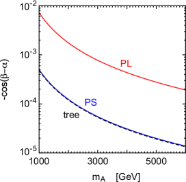
Figure 1: $\cos(\beta-\alpha)$ is plotted as a function of $m_{A}$ with $\tan\beta=35$, $M_{3}=-\mu=5\,{\rm TeV}$, and the approximate GUT relation among gaugino masses (see Eq. (3.2)). All the sfermion masses are assumed to be universal at $M_{\rm SUSY}$, and are also taken to be $5\,{\rm TeV}$. The red and blue lines correspond to the cases of the PL and PS solutions of $A_{t}$, respectively. The black dashed line is the tree-level value.

Denoting $h\bar{f}f$ coupling (with $f$ being the SM fermions) as

$$-\mathcal{L}_{h\bar{f}f}\equiv g_{h\bar{f}f}h\bar{f}f,$$ (2.12)

we obtain the $h\bar{b}b$ coupling constant as

$$g_{h\bar{b}b} =-\left(\frac{\sin\alpha}{\cos\beta}\right)\frac{1-\Delta_{b}\cot\alpha\cot\beta}{1+\Delta_{b}}g_{h\bar{b}b}^{\rm(SM)}$$

$$=\left[\sin(\beta-\alpha)-\frac{\tan\beta-\Delta_{b}\cot\beta}{1+\Delta_{b}}\cos(\beta-\alpha)\right]g_{h\bar{b}b}^{\rm(SM)},$$ (2.13)

where the superscript “(SM)” is used for the SM prediction. When $m_{A}$ is relatively large, $\sin(\beta-\alpha)$ is almost unity, while the second term proportional to $\cos(\beta-\alpha)$ induces a sizable deviation from the SM value. Similar relation holds for $h\bar{\tau}\tau$ vertex, and $\Delta_{\tau}$ is approximately given by

$$\Delta_{\tau} \simeq-\frac{3\alpha_{2}}{8\pi}M_{2}\mu\tan\beta\,I(m_{\tilde{\tau}_{L}}^{2},M_{2}^{2},\mu^{2}),$$ (2.14)

with $M_{2}$ being the Wino mass. Quantitatively, $\Delta_{\tau}$ is smaller than $\Delta_{b}$ in the parameter space of our study. As we will see later, $\Gamma(h\rightarrow\bar{b}b)$ and $\Gamma(h\rightarrow\bar{\tau}\tau)$ may show sizable deviations from the SM predictions even if $m_{A}$ is above TeV.

The $h\bar{t}t$ coupling constant is obtained as

$$g_{h\bar{t}t} =\left(\frac{\cos\alpha}{\sin\beta}\right)\frac{1-\Delta_{t}\tan\alpha\tan\beta}{1+\Delta_{t}}g_{h\bar{t}t}^{\rm(SM)}$$

$$=\left[\sin(\beta-\alpha)+\frac{\cot\beta-\Delta_{t}\tan\beta}{1+\Delta_{t}}\cos(\beta-\alpha)\right]g_{h\bar{t}t}^{\rm(SM)}.$$ (2.15)

The deviation from the SM value mainly comes from the second term in the bracket and is not enhanced by $\tan\beta$, since $\Delta_{t}$ is proportional to $\cot\beta$.

The gauge-boson final states are also important. In order to calculate the partial decay widths of the Higgs to gauge bosons, we have modified FeynHiggs 2.10.2 package to properly take account of the effect of non-holomorphic correction to the Higgs interaction. We have also modified the package to take the $\alpha_{\rm eff}$ approximation [28] for calculating the partial widths, in which the renormalization scale of the Higgs wave functions is set to be $p^{2}=0$, and the effects of radiative corrections are included in the mixing between the light and heavy Higgs bosons. Then, as we will see below, the partial decay widths show proper decoupling behavior in the large $m_{A}$ limit.

The processes induced by triangle loops, $h\rightarrow gg$ and $\gamma\gamma$, have been important for the Higgs discovery at the LHC. They are also important in studying new particles that couple to the Higgs boson. In SUSY models, the stop and sbottom loops contribute to the $hgg$ coupling. It is expressed by an approximate formula (cf. Refs. [25, 26, 27])

$$\frac{g_{hgg}}{g^{\rm(SM)}_{hgg}}\simeq\frac{g_{h\bar{t}t}}{g_{h\bar{t}t}^{\rm(SM)}}+\sum_{f=t,b}\frac{m_{f}^{2}}{4(1+\Delta_{f})^{2}}\left(\frac{1}{m^{2}_{\tilde{f}_{1}}}+\frac{1}{m^{2}_{\tilde{f}_{2}}}-\frac{X^{2}_{f}}{m^{2}_{\tilde{f}_{1}}m^{2}_{\tilde{f}_{2}}}\right),$$ (2.16)

up to $D$-term and bottom-loop contributions. Here, $X_{b}=A_{b}-\mu\tan\beta$. In the right-hand side, the first term comes from the top loop, while the second term is given by the stop and sbottom loops. The correction is positive in the non-mixing limit (i.e., $X_{f}\rightarrow 0$), whereas it becomes negative when the mixing terms are sizable. We also note here that $hVV$ couplings (with $VV=W^{+}W^{-}$ and $ZZ$) are approximately given by $g_{hVV}/g_{hVV}^{\rm(SM)}=\sin(\beta-\alpha)$. This ratio is very close to unity, and hence the deviations in these modes are very small.

2.2 Constraints

Before discussing the possibility of observing a deviation of the Higgs partial widths from the SM prediction at future colliders, we summarize phenomenological constraints on the MSSM parameter space which are adopted in our analysis.

2.2.1 $B_{s}\to\mu^{+}\mu^{-}$

In the SM, the flavor-changing decay, $B_{s}\to\mu^{+}\mu^{-}$, proceeds by virtual exchanges of the $Z$ and $W$ bosons. They are suppressed by the final-state helicity. In contrast, SUSY contributions can be enhanced considerably by large $\tan\beta$, when virtual exchanges of the heavy Higgs boson contribute to the decay [30, 31]. The branching ratio is expressed as [32, 33, 34, 35]

$${\rm Br}(B_{s}\to\mu^{+}\mu^{-})= \frac{G_{F}^{2}\alpha^{2}}{64\pi^{3}}f_{B_{s}}^{2}m_{B_{s}}^{3}\tau_{B_{s}}\left|V_{tb}V_{ts}^{*}\right|^{2}\sqrt{1-\frac{4m_{\mu}^{2}}{m_{B_{s}}^{2}}}$$

$$\times\left[\left(1-\frac{4m_{\mu}^{2}}{m_{B_{s}}^{2}}\right)\left|C_{Q1}-C_{Q1}^{\prime}\right|^{2}+\left|\left(C_{Q2}-C_{Q2}^{\prime}\right)+\frac{2m_{\mu}}{m_{B_{s}}}\left(C_{10}-C_{10}^{\prime}\right)\right|^{2}\right],$$ (2.17)

where $G_{F}$ is the Fermi constant, $m_{B_{s}}$ is the $B_{s}$-meson mass, $f_{B_{s}}$ is the decay constant of $B_{s}$, $m_{\mu}$ is the muon mass, $\tau_{B_{s}}$ is the lifetime of $B_{s}$, and $V_{ij}$ is Cabbino-Kobayashi-Maskawa matrix element. In the above expression, $C_{10}$, $C_{Q1}$ and $C_{Q2}$ are the Wilson coefficients of the effective operators, $\mathcal{O}_{i}\propto(\bar{s}\gamma_{\mu}P_{L}b)(\bar{\ell}\gamma^{\mu}\gamma_{5}\ell)$, $(\bar{s}P_{R}b)(\bar{\ell}\ell)$, and $(\bar{s}P_{R}b)(\bar{\ell}\gamma_{5}\ell)$, respectively, while $C_{i}^{\prime}$ are obtained by flipping chiralities, $R\leftrightarrow L$. Among them, the SM contribution appears only in $C_{10}$. Including higher order contributions and taking account of effects of the $B_{s}\text{-}\bar{B}_{s}$ oscillation, the SM prediction becomes [36]

$${\rm Br}(B_{s}\to\mu^{+}\mu^{-})_{\rm SM}=(3.65\pm 0.23)\times 10^{-9}.$$ (2.18)

This can be compared with the LHCb measurements [37]

$${\rm Br}(B_{s}\to\mu^{+}\mu^{-})_{\rm LHCb}=(2.8^{+0.7}_{-0.6})\times 10^{-9}.$$ (2.19)

Defining $\Delta{\rm Br}(B_{s}\to\mu^{+}\mu^{-})\equiv{\rm Br}(B_{s}\to\mu^{+}\mu^{-})-{\rm Br}(B_{s}\to\mu^{+}\mu^{-})_{\rm SM}$, where the first term in the right-hand side includes both the SUSY and SM contributions, the 95% C.L. bound is estimated as

$$-2.3\times 10^{-9}<\Delta{\rm Br}(B_{s}\to\mu^{+}\mu^{-})<0.6\times 10^{-9}.$$ (2.20)

We will adopt this constraint in our numerical analysis.

Even when superparticles are heavy, they affect the branching ratio through non-holomorphic contributions to the heavy Higgs couplings. Including radiative corrections and diagonalizing the quark mass matrices, effective couplings of the heavy Higgs bosons to the down-type fermions become [30, 31]

$$\mathcal{L}_{\rm eff}\simeq \frac{gm_{b}}{\sqrt{2}m_{W}\cos\beta}\frac{\Delta_{\rm FC}}{(1+\Delta_{b})(1+\Delta_{0})}V_{tb}V_{ts}^{*}\,(\bar{s}_{L}b_{R})\left(H+iA\right)$$

$$+\frac{gm_{\ell}}{\sqrt{2}m_{W}\cos\beta}\frac{1}{1+\Delta_{\ell}}(\bar{\ell}_{L}\ell_{R})\left(H+iA\right)+{\rm h.c.},$$ (2.21)

where $\Delta_{0}=\Delta_{b}-\Delta_{\rm FC}$. The flavor-changing coupling is induced by $\Delta_{\rm FC}$ as

$$\Delta_{\rm FC}=\frac{y_{t}^{2}}{16\pi^{2}}\mu A_{t}\tan\beta\,I(m_{\tilde{t}_{1}}^{2},m_{\tilde{t}_{2}}^{2},\mu^{2}).$$ (2.22)

Here, soft scalar masses are assumed to be universal in generation, and $\Delta_{\ell}$ is obtained by substituting $\tilde{\tau}\rightarrow\tilde{\ell}$ in Eq. (2.14). Then, the Wilson coefficients receive Higgs-mediated contributions,

$$C_{Q1}\simeq-C_{Q2}\simeq-\frac{m_{t}^{2}m_{b}m_{\mu}}{4\sin^{2}\theta_{W}m_{W}^{2}m_{A}^{2}}\frac{\tan^{3}\beta}{(1+\Delta_{b})^{2}}\frac{\mu A_{t}}{m_{\tilde{t}}^{2}}x_{\tilde{t}\mu}I(x_{\tilde{t}\mu},x_{\tilde{t}\mu},1),$$ (2.23)

where $m_{b}$ is the bottom-quark mass, $\theta_{W}$ is the Weinberg angle, and $x_{\tilde{t}\mu}\equiv m_{\tilde{t}}^{2}/\mu^{2}$. The non-holomorphic correction $\Delta_{\rm FC}$ as well as $\Delta_{b}$ does not decouple even for very heavy superparticles. We will see later that the corrections to ${\rm Br}(B_{s}\to\mu^{+}\mu^{-})$ can be sizable and that the constraint excludes some part of the parameter space of our interest.

The branching ratio of the inclusive decay of $b\to s\gamma$ may also be sensitive to the non-decoupling contributions to the (charged) Higgs boson. In the numerical analysis, defining $\Delta{\rm Br}(b\to s\gamma)\equiv{\rm Br}(b\to s\gamma)-{\rm Br}(b\to s\gamma)_{\rm SM}$, we adopt the 95% C.L. bound,

$$-3.6\times 10^{-5}<\Delta{\rm Br}(b\to s\gamma)<9.2\times 10^{-5}.$$ (2.24)

where the experimental value ${\rm Br}(b\to s\gamma)_{\rm exp}=(3.43\pm 0.21\pm 0.07)\times 10^{-4}$ [38] and the SM prediction ${\rm Br}(b\to s\gamma)_{\rm SM}=(3.15\pm 0.23)\times 10^{-4}$ [39] are combined. At the current accuracies, $B_{s}\to\mu^{+}\mu^{-}$ imposes more stringent bound on the parameter space than $b\to s\gamma$ except when superparticles are light.

In the numerical analysis, SuperIso 3.4 [40] is used for evaluating the SUSY contributions to the branching ratios as well as the SM predictions. In our analysis, we assume that the squark masses are universal in generations. If the squark masses are non-universal, there are extra contributions to $\Delta_{\rm FC}$, and the flavor constraints are affected (see e.g., Ref. [41]). Such a non-universality is expected even in the model with the universal scalar masses at the GUT scale. Thus, it should be noted that the flavor constraints that we will show below are just for a particular choice of the squark-mass parameters and may change if the squark mass matrices have non-universal structures.

2.2.2 Vacuum stability

With sufficiently large $|A_{t}|$, CCB vacua arise, and the minimum of the scalar potential with the correct EWSB becomes a false vacuum [42, 43, 44, 45]. When $|\mu|\ll|A_{t}|$, stop and the up-type Higgs fields acquire large VEVs at the CCB vacua, while the VEVs of other fields are relatively small. Recently, the decay rate of the SM-like vacuum has been studied in detail for such a case [46, 47, 48, 49]. On the other hand, if $\mu$ is as large as the stop masses, the down-type Higgs boson also has a large VEV at the CCB vacua due to the tri-linear scalar coupling among stops and the down-type Higgs, which is proportional to $y_{t}\mu$. The vacuum stability condition is important in such a case because significant deviations of the Higgs partial widths from the SM prediction may occur. In order to study the SM-like vacuum stability, we consider the tree-level scalar potential in the field space involving $\tilde{t}_{L}$, $\tilde{t}_{R}$, $h_{u}$ and $h_{d}$ (which are canonically normalized scalar fields embedded in the left-handed stop, right-handed stop, the up-type Higgs and the down-type Higgs, respectively).

The relevant part of the potential is given by

$$V= \frac{1}{2}m_{11}^{2}\,h_{d}^{2}+\frac{1}{2}m_{22}^{2}\,h_{u}^{2}-m_{12}^{2}\,h_{d}h_{u}+\frac{1}{2}m_{\tilde{Q}}^{2}\,\tilde{t}_{L}^{2}+\frac{1}{2}m_{\tilde{U}}^{2}\,\tilde{t}_{R}^{2}$$

$$+\frac{1}{\sqrt{2}}y_{t}(A_{t}h_{u}-\mu h_{d})\tilde{t}_{L}\tilde{t}_{R}+\frac{1}{4}y_{t}^{2}(\tilde{t}_{L}^{2}\tilde{t}_{R}^{2}+\tilde{t}_{L}^{2}h_{u}^{2}+\tilde{t}_{R}^{2}h_{u}^{2})$$

$$+\frac{1}{24}g_{3}^{2}(\tilde{t}_{L}^{2}-\tilde{t}_{R}^{2})^{2}+\frac{1}{32}g_{2}^{2}(h_{u}^{2}-h_{d}^{2}-\tilde{t}_{L}^{2})^{2}+\frac{1}{32}g_{Y}^{2}\left(h_{u}^{2}-h_{d}^{2}+\frac{1}{3}\tilde{t}_{L}^{2}-\frac{4}{3}\tilde{t}_{R}^{2}\right)^{2},$$ (2.25)

where

$$m_{11}^{2} =m_{A}^{2}\sin^{2}\beta-\frac{1}{2}m_{Z}^{2}\cos 2\beta,$$ (2.26)

$$m_{22}^{2} =m_{A}^{2}\cos^{2}\beta+\frac{1}{2}m_{Z}^{2}\cos 2\beta,$$ (2.27)

$$m_{12}^{2} =\frac{1}{2}m_{A}^{2}\sin 2\beta.$$ (2.28)

When the CCB vacua become deeper than the SM-like vacuum, the latter is not stable. The vacuum decay rate per unit volume is calculated in the semi-classical approximation, and is expressed as

$$\Gamma/V=C\exp(-S_{E}),$$ (2.29)

where $S_{E}$ is the Euclidean action of the so-called bounce solution [50, 51]. For the decay of the SM-like vacuum, $C$ is estimated to be $\sim(100\,{\rm GeV})^{4}$. In order for the lifetime of the SM-like vacuum to be longer than the present age of the universe, the Euclidean action is required to satisfy

$$S_{E}\gtrsim 400.$$ (2.30)

In our numerical analysis, CosmoTransition 2.0a1 [52] is used to find the bounce solution in the four-dimensional field space parameterized by $h_{d}$, $h_{u}$, $\tilde{t}_{L}$ and $\tilde{t}_{R}$, and to calculate the Euclidean bounce action $S_{E}$. The calculation is done at zero temperature, and therefore thermal effects are not taken into account. The model parameters such as the tri-linear and top Yukawa couplings are evaluated at the SUSY scale $M_{\rm SUSY}$.

In Fig. 2 we show the contours of constant $S_{E}$ for the PS and PL solutions on $m_{A}$ vs. $\mu$ plane. Here, $m_{\tilde{Q}}=m_{\tilde{U}}=M_{3}=5\,{\rm TeV}$, while sfermion masses, $m_{\tilde{D}}$, $m_{\tilde{L}}$ and $m_{\tilde{E}}$, are taken to be ${\rm max}(m_{\tilde{U}},\mu)$ (see Sec. 3). In each plot, the region between the solid (dashed) green lines satisfies $S_{E}>400$ ($300$). For the PS solution, these lines appear only for $|\mu|>10\,{\rm TeV}$. On the other hand, the upper bound on $|\mu|$ is comparable to the stop masses for the PL solution.

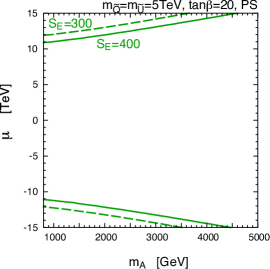
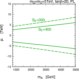
Figure 2: Contours of $S_{E}=300$ and $400$ on $m_{A}$ vs. $\mu$ plane for the PS and PL solutions of $A_{t}$. Here, $m_{\tilde{Q}}=m_{\tilde{U}}=M_{3}=5\,{\rm TeV}$, $m_{\tilde{D}}=m_{\tilde{L}}=m_{\tilde{E}}=\max(m_{\tilde{U}},|\mu|)$, and $\tan\beta=20$.

The tree-level potential Eq. (2.25) is used for our numerical analysis. Radiative corrections may change the scalar potential particularly around the SM-like vacuum. In order to study their effects, we also estimated the decay rate of the SM-like vacuum by including the top-stop and bottom-sbottom one-loop correction to the Higgs potential. We found that the Euclidean action tends to increase by about 10 – 20% for $S_{E}\sim 400$ from that of the tree-level potential. In order to see the sensitivity of $S_{E}$ to $\mu$, we show the contours of $S_{E}=300$ in the same plot.

When both $\mu$ and $\tan\beta$ are large, we might have to consider other CCB vacua in the sbottom-Higgs direction, which is driven by the tri-linear coupling of $y_{b}(A_{b}h_{d}-\mu h_{u})\tilde{b}_{L}\tilde{b}_{R}/\sqrt{2}$ (where $\tilde{b}_{L}$ and $\tilde{b}_{R}$ are left- and right-handed sbottoms, respectively) (cf. Ref. [41]). If both $\mu$ and $A_{b}$ are large, the bottom Yukawa coupling can be enhanced not only by $\tan\beta$ but also by $(1+\Delta_{b})^{-1}$ (see Eq. (2.31)). However, when the squark masses are universal, such a parameter region is already excluded by the other constraints discussed in this section. Therefore we do not consider the constraint coming from the CCB vacuum involving the sbottom sector in this paper.

2.2.3 Bottom Yukawa coupling

When $\tan\beta$ is very large, the bottom Yukawa coupling is sizable. We can impose an upper bound on $\tan\beta$ by requiring perturbativity of the Yukawa coupling constants up to, for instance, the GUT scale. In the MSSM, the bottom Yukawa coupling constant $y_{b}$ is proportional to $(1+\Delta_{b})^{-1}$, and hence, $y_{b}$ is enhanced when $\Delta_{b}$ is negative (see Eq. (2.4)). Consequently, the bound on $\tan\beta$ is more severe when $\Delta_{b}<0$.

In our numerical analysis, we estimate the bottom Yukawa coupling constant using the following relation:

$$y_{b}(M_{\rm SUSY})\simeq\frac{\sqrt{2}m_{b}(M_{\rm SUSY})}{v\cos\beta(1+\Delta_{b})}.$$ (2.31)

Then, we follow the evolutions of coupling constants by solving the renormalization group equations at the one-loop level and impose a condition that the bottom Yukawa coupling is perturbative up to the grand unified theory (GUT) scale $M_{\rm GUT}$. Numerically, we require

$$\left|y_{b}(M_{\rm GUT})\right|<1,$$ (2.32)

where we take $M_{\rm GUT}=2\times 10^{16}\,{\rm GeV}$. This constraint excludes a large $\tan\beta$ region especially when $\Delta_{b}<0$. Notice that $\Delta_{b}$ is a non-decoupling parameter, and hence, this constraint is important even in the limit of heavy superparticles.

3 Higgs Partial Decay Widths

In this section,we discuss the partial decay width of the lightest Higgs boson $h$. We define the ratio of the partial decay width of the lightest Higgs boson to that of the SM prediction:

$$R_{F}\equiv\frac{\Gamma(h\rightarrow F)}{\Gamma^{\rm(SM)}(h\rightarrow F)},$$ (3.1)

where $F$ denotes a specific final state. In the following, we show how much $R_{F}$ can deviate from the SM prediction ($R_{F}=1$) for various final states. As we have mentioned, FeynHiggs 2.10.2 is used to calculate the partial decay widths of the Higgs boson, in which full one-loop contributions are taken into account for the fermionic final states. In the package, a resummation of the $\Delta_{b}$ corrections is also included in calculating the partial decay width for $h\rightarrow\bar{b}b$ [53].

In our numerical calculation, we adopt (approximate) GUT relation among the $SU(3)_{C}$, $SU(2)_{L}$, and $U(1)_{Y}$ gaugino masses:

$$M_{3}(M_{\rm SUSY})=3M_{2}(M_{\rm SUSY})=6M_{1}(M_{\rm SUSY}).$$ (3.2)

All the phases in the MSSM parameters are assumed to be negligible, and we adopt the convention of $M_{3}>0$. For simplicity, we also assume that the sfermion masses are universal with respect to the generation indices.

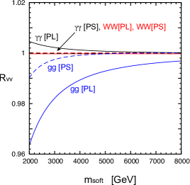
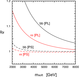
Figure 3: $R_{VV}$ (left) and $R_{\bar{f}f}$ (right) are shown as functions of $m_{\rm soft}$; here all the fermion masses, $M_{3}$, and $|\mu|$ are equal to $m_{\rm soft}$, and $\tan\beta=40$. (The sign of $\mu$ is taken to be negative, while Wino and Bino masses are given by using the approximate GUT relation (3.2).) In the left (right) plot, the black, red, and blue lines correspond to $h\rightarrow\gamma\gamma$ ($\bar{b}b$), $h\rightarrow W^{+}W^{-}$ ($\bar{\tau}\tau$), and $h\rightarrow gg$, respectively. The solid (dashed) lines correspond to the PL (PS) solutions of $A_{t}$. Note that the constraints in Sec. 2.2 are not taken into account.

First, we show the soft mass dependence of $R_{F}$ without taking the phenomenological constraints into account. In Fig. 3, $R_{F}$ are shown for $F=\gamma\gamma$, $W^{+}W^{-}$, $gg$, $\bar{b}b$, and $\bar{\tau}\tau$ as functions of $m_{\rm soft}$, taking $M_{3}=m_{A}=-\mu=m_{\tilde{Q}}=m_{\tilde{U}}=m_{\tilde{D}}=m_{\tilde{L}}=m_{\tilde{E}}\equiv m_{\rm soft}$ and $\tan\beta=40$. By choosing negative $\mu$ with $|\mu|\sim m_{\rm soft}$, the correction to the bottom Yukawa coupling becomes significant.

Remarkably, even though $m_{\rm soft}$ is around several TeV, the partial decay widths for $F=\bar{b}b$, $\bar{\tau}\tau$ and $gg$ deviate from the SM prediction by more than $\mathcal{O}(1)$ % for the PL solution. However, SUSY contributions to the other widths are smaller. Note that $R_{\bar{b}b}-1$ is as about twice as $R_{\bar{\tau}\tau}-1$ for the PL solution, which is due to the difference between $\Delta_{b}$ and $\Delta_{\tau}$. We also note here that the partial decay widths have an appropriate decoupling behaviour, i.e., $\Gamma(h\rightarrow F)\rightarrow\Gamma^{\rm(SM)}(h\rightarrow F)$ as the masses of superparticles and the heavy Higgs bosons become infinitely large.

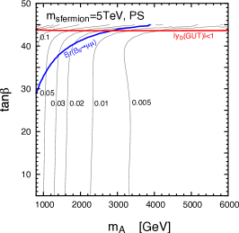
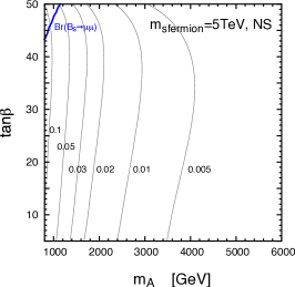
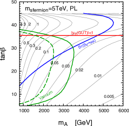
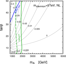
Figure 4: Contours of $R_{\bar{b}b}-1$ are shown for the PS, NS, PL, and NL solutions of $A_{t}$. Here, all the sfermion masses, $M_{3}$, and $|\mu|$ are taken to be $5\,{\rm TeV}$, and the sign of $\mu$ is set to be negative. The left regions of the blue lines are excluded by ${\rm Br}(B_{s}\to\mu^{+}\mu^{-})$, while those of the green solid (dashed) lines are constrained by the vacuum stability condition, $S_{E}>400$ (360). The bottom Yukawa coupling becomes non-perturbative below the GUT scale in the region above the red line.

Next, let us include the phenomenological constraints discussed in Sec. 2.2. In Fig. 4, contours of $R_{\bar{b}b}-1$ are shown on $m_{A}$ vs. $\tan\beta$ plane. Here, all the sfermion masses, $M_{3}$, and $|\mu|$ are set to be $5\,{\rm TeV}$. In the cases of the PS and PL solutions, the contours end at around $\tan\beta\sim 45$. This is because, when $\tan\beta$ is large, there is no solution for $A_{t}$ to satisfy $m_{h}=125.7\,{\rm GeV}$. The bottom-sbottom loop contribution interferes destructively with the top-stop contribution, and thus, larger (smaller) $A_{t}$ is required for the PS (PL) solution. Then, $A_{t}^{({\rm PS})}$ and $A_{t}^{({\rm PL})}$ merge into a single solution at certain $\tan\beta$, which is the value where the top-stop contributions cannot raise the Higgs mass anymore for fixed $m_{\rm soft}$. Note that, $\Delta_{b}$ is negative when $\mu<0$ and $A_{t}>0$. In such a case, $y_{b}$ is significantly larger than the tree-level value, and thus, the bottom-sbottom loop contributions are enhanced.

In Fig. 4, the constraints from ${\rm Br}(B_{s}\to\mu^{+}\mu^{-})$, the vacuum stability, and the perturbativity of the bottom Yukawa couplings are shown. Wide parameter region is excluded when $A_{t}$ is large, i.e., in the PL and NL panels. The constraints from ${\rm Br}(B_{s}\to\mu^{+}\mu^{-})$ and the vacuum stability become weaker for large $m_{A}$, while that from the perturbativity is not. For the PL solution, the constraints from ${\rm Br}(B_{s}\to\mu^{+}\mu^{-})$ and the vacuum stability change drastically as we vary $\tan\beta$ for $\tan\beta\gtrsim 30$, where the bottom Yukawa coupling is much larger than the tree-level value.

	LHC [3]		ILC [54]				TLEP [3]
$\sqrt{s}$ [GeV]	1400	1400	250	500	1000		240	350
$\int\!dt\,\mathcal{L}$ [$\,{\rm fb^{-1}}$]	300	3000	250	500	1000	2500	10000	+2600
$\gamma\gamma$	10 – 14	4 – 10	38	17	5.8	3.8	3.4	3.0
$gg$	12 – 16	6 – 10	12	4.0	1.6	1.2	2.2	1.6
$\bar{b}b$	20 – 26	8 – 14	9.4	1.9	0.78	0.64	1.8	0.84
$\bar{\tau}\tau$	12 – 16	4 – 10	10	3.8	1.6	1.3	1.9	1.1

Table 1: Expected accuracies of the determinations of the partial decay widths of the Higgs boson in units of percents [3, 54]. The accuracies of the widths are assumed to be twice the accuracies of the determinations of couplings.

Even if the masses of superparticles are relatively large (i.e., $5\,{\rm TeV}$), $R_{\bar{b}b}-1$ can be as large as $\mathcal{O}(1)$ %. Such a large deviation may be within the reach of future collider experiments. Expected accuracies at the future experiments have been discussed (see Table 1-16 of Ref. [3] and Ref. [54]); the numbers are summarized in Table 1. The accuracies of $\delta\Gamma(h\rightarrow\bar{b}b)=0.64\%$, $\delta\Gamma(h\rightarrow\bar{\tau}\tau)=1.1\%$, and $\delta\Gamma(h\rightarrow gg)=1.2\%$ are claimed to be achievable at $e^{+}e^{-}$ colliders ultimately. Therefore, it is found that, even if the superparticles are kinematically unaccessible at the LHC, we may observe the MSSM signal by studying the partial decay widths of $h$ in detail.

For the PL solution, it is also found that the partial width of $h\rightarrow\bar{b}b$ can deviate from the SM prediction by about 2% even for $m_{A}=6\,{\rm TeV}$. On the other hand, we checked that $R_{\bar{\tau}\tau}$ is smaller by about 1% than $R_{\bar{b}b}$ at the same parameter point, because the non-holomorphic correction $|\Delta_{b}|$ is bigger than $|\Delta_{\tau}|$ at this model point. When $\tan\beta$ is smaller, the difference between $R_{\bar{b}b}$ and $R_{\bar{\tau}\tau}$ decreases, since $\Delta_{b}$ is approximately proportional to $\tan\beta$; in such a case both $R_{\bar{b}b}$ and $R_{\bar{\tau}\tau}$ are well approximated by $(\sin\alpha/\cos\beta)^{2}$.

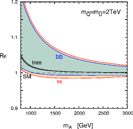
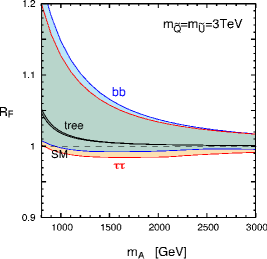
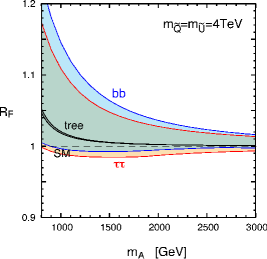
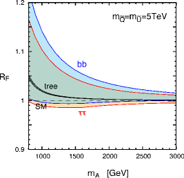
Figure 5: The ranges of $R_{\bar{b}b}$ (blue) and $R_{\bar{\tau}\tau}$ (red) with small $|A_{t}|$ solutions (i.e, the PS and NS solutions for $A_{t}$). We take $m_{\tilde{Q}}=m_{\tilde{U}}=M_{3}=2$, 3, 4 and $5\,{\rm TeV}$. Other sfermion masses are set to be $\max(m_{\tilde{Q}},|\mu|)$. The partial widths are constrained by ${\rm Br}(B_{s}\to\mu^{+}\mu^{-})$, the vacuum stability condition ($S_{E}>400$), and the perturbativity of the bottom Yukawa coupling ($|y_{b}({\rm GUT})|<1$). The black region corresponds to the tree-level prediction for $\tan\beta=5$–$50$. The black dashed line is the SM prediction.

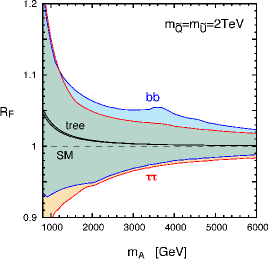
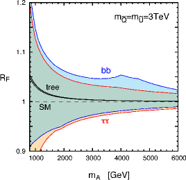
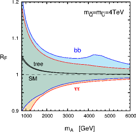
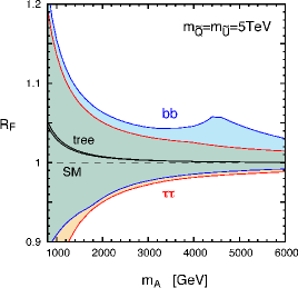
Figure 6: Same as Fig. 5, but with all the solutions of $A_{t}$.

Let us see how much $R_{\bar{b}b}$ and $R_{\bar{\tau}\tau}$ can change in the parameter space consistent with the phenomenological constraints. We have performed the scan in the following parameter space of the MSSM:

• $m_{\tilde{Q}}=m_{\tilde{U}}=M_{3}=2$, $3$, $4$, and $5\,{\rm TeV}$,

• $m_{\tilde{D}}=m_{\tilde{L}}=m_{\tilde{E}}=\max(m_{\tilde{U}},|\mu|)$,

• $A_{t}=A_{t}^{({\rm NS})}$, $A_{t}^{({\rm NL})}$, $A_{t}^{({\rm PS})}$, $A_{t}^{({\rm PL})}$,

• $0.8\,{\rm TeV}\leq m_{A}\leq 6\,{\rm TeV}$,

• $-5\leq\mu/m_{\tilde{U}}\leq-0.5$, or $0.5\leq\mu/m_{\tilde{U}}\leq 5$,

• $5\leq\tan\beta\leq 50$.

Here, $A_{t}$ is determined to satisfy $m_{h}=125.7\,{\rm GeV}$. The other tri-linear couplings (e.g., $A_{b}$ and $A_{\tau}$) are assumed to be equal to $A_{t}$; we checked that our numerical results are insensitive to this assumption. We take $m_{\tilde{Q}}=m_{\tilde{U}}=M_{3}$, while sfermion masses other than $m_{\tilde{Q}}$ and $m_{\tilde{U}}$ are set to be equal to $\max(m_{\tilde{U}},|\mu|)$. We have checked that $R_{\bar{b}b}$ and $R_{\bar{\tau}\tau}$ are almost insensitive to these scalar masses unless they are very small. However, when $|\mu|$ is much larger than $m_{\tilde{D}}$, $m_{\tilde{L}}$, and $m_{\tilde{E}}$, bottom and stau mixings become sizable which causes additional complexity to our parameter scan, and/or lighter stau become tachyonic. The values of $m_{\tilde{D}}$, $m_{\tilde{L}}$, and $m_{\tilde{E}}$ are chosen to avoid this problem.

If $|\mu|$ would become much larger than squark masses (e.g., $|\mu|/m_{\tilde{U}}\gg 5$), the Higgs partial widths could deviate from the SM prediction sizably, since the Higgs mixing angle would be enhanced by radiative corrections. However, the vacuum stability condition excludes significant amount of the parameter region with large $|\mu|$, as we have shown in Fig. 2. In our scan, we set $|\mu|/m_{\tilde{U}}\leq 5$; this upper bound is large enough to cover the whole region allowed by the vacuum stability.

In Figs. 5 and 6, we show the minimal and maximal values of $R_{\bar{b}b}$ and $R_{\bar{\tau}\tau}$ as functions of $m_{A}$ and $m_{\rm soft}$, taking into account the phenomenological constraints discussed in the previous section. Fig. 5 corresponds to the small $A_{t}$ solutions (NS and PS). The largest and smallest values of $R_{\bar{b}b}$ and $R_{\bar{\tau}\tau}$ are achieved when $|\mu|$ and $\tan\beta$ are large and are marginally allowed by the phenomenological constraints. The deviations mainly come from radiative corrections to the Higgs mixing angle and $\Delta_{b}$. In particular, the maximal value of $R_{\bar{b}b}$ is larger than that of $R_{\bar{\tau}\tau}$ for large $m_{\tilde{Q}}=m_{\tilde{U}}$. As discussed earlier, $\Delta_{b}$ becomes negative and sizable with $\mu<0$, which results in a significant enhancement of $R_{\bar{b}b}$.

Fig. 6 shows the minimal and maximal values of $R_{\bar{b}b}$ and $R_{\bar{\tau}\tau}$, taking all the solutions of NS, PS, NL, and PL into consideration. They change significantly compared to Fig. 5. The partial widths become extremum when $A_{t}$ takes the NL or PL solution except the maximal value for small $m_{A}$. For $m_{A}\lesssim 1\,{\rm TeV}$, the NS or PS solutions give the maximal value, since the phenomenological constraints, especially the vacuum stability condition, are too severe for the NL and PL solutions (see Fig. 4). As in the case of Fig. 5, the maximal value of $R_{\bar{b}b}$ is much larger than that of $R_{\bar{\tau}\tau}$ because $|\Delta_{b}|\gg|\Delta_{\tau}|$. The maximal value of $R_{\bar{b}b}$ has a non-trivial bump-like structure. When $m_{A}$ is small, medium (i.e., around the peak of the bump), and large, the partial decay width is bounded by the vacuum stability, flavor constraint, and the perturbativity of $y_{b}$, respectively.

The measurement of the Higgs couplings may provide an evidence of BSM, because the values of $R_{\bar{b}b}$ and $R_{\bar{\tau}\tau}$ may show significant deviation from the SM prediction. In future experiments, the partial decay widths of $h\rightarrow\bar{b}b$ and $h\rightarrow\bar{\tau}\tau$ may be measured at the $\lesssim 1\%$ level (see Table 1). In the case of the PS and NS solutions, $R_{\bar{b}b}-1$ can be as large as 2% (3%) if $m_{A}$ is $2.7\,{\rm TeV}$ ($2.2\,{\rm TeV}$) for $m_{\rm soft}=2\,{\rm TeV}$, and $2.6\,{\rm TeV}$ ($2.1\,{\rm TeV}$) for $m_{\rm soft}=5\,{\rm TeV}$. On the other hand, $R_{\bar{\tau}\tau}-1$ becomes larger than 2% (3%) when $m_{A}$ is smaller than $3.0\,{\rm TeV}$ ($2.4\,{\rm TeV}$) for $m_{\rm soft}=2\,{\rm TeV}$, and $2.1\,{\rm TeV}$ ($1.8\,{\rm TeV}$) for $m_{\rm soft}=5\,{\rm TeV}$. Including the PL and NL solutions, deviations of $2$ – $3$% level are achieved with larger value of $m_{A}$. For example, with $m_{\rm soft}=5\,{\rm TeV}$, $R_{\bar{b}b}-1=3\%$ can be achieved with $m_{A}=6.0\,{\rm TeV}$.

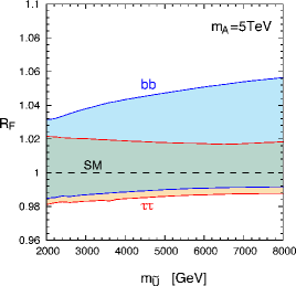
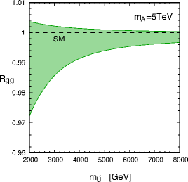
Figure 7: The ranges of $R_{\bar{f}f}$ (left) and $R_{gg}$ (right) are shown as functions of $m_{\tilde{U}}$. The parameters are scanned in the same manner as Fig. 6, but $m_{A}$ is fixed to be $5\,{\rm TeV}$ while $m_{\tilde{U}}$ is varied. Here, all the solutions of $A_{t}$ are included in the scan with imposing the phenomenological constraints discussed in Sec. 2.2. The black dashed line is the SM prediction.

In Fig. 7, we show the sfermion mass dependence of $R_{F}$ with taking the phenomenological constraints into account. The parameter scan is performed in the same setup as Fig. 6, but $m_{\tilde{U}}$ is varied. Here, $m_{A}$ is fixed to be $5\,{\rm TeV}$. In the left plot, the minimal and maximal values of $R_{\bar{b}b}$ and $R_{\bar{\tau}\tau}$ are shown. They are achieved by the PL or NL solution. Since $m_{A}$ is fixed, the decoupling behaviour is not observed. Rather, the non-decoupling contribution to $\Delta_{b}$ enhances $R_{\bar{b}b}$ as $m_{\tilde{U}}$ increases, since larger $|A_{t}|$ is required to satisfy $m_{h}=125.7\,{\rm GeV}$ for the solutions. On the other hand, it is found that radiative corrections to the Higgs mixing angle do not change so much even if $m_{\tilde{U}}$ increases.

In the right panel of Fig. 7, the minimal and maximal values of $R_{gg}$ are displayed. The maximal value occurs for the PS or NS solution, while the minimal value is achieved by the PL or NL solution. We can see the decoupling behavior, i.e., $R_{gg}$ approaches to unity as $m_{\tilde{U}}$ increases. The partial decay width of $h\rightarrow gg$ can deviate from the SM prediction by about 3% for $m_{\tilde{U}}=2\,{\rm TeV}$, while it decreases rapidly and becomes 1% for $m_{\tilde{U}}=3.7\,{\rm TeV}$. We have also checked that these values do not change so much for $m_{A}=8\,{\rm TeV}$. (However, they change significantly if $m_{A}$ is smaller, since the phenomenological constraints exclude the parameter space severely.) According to Table 1, the partial width of $h\rightarrow gg$ is expected to be measured at the $1.2\%$ accuracy in future experiments. Thus, as far as superparticles are relatively light, we may observe a signal of the MSSM in the measurements of this partial width even if the heavier Higgses are out of the reach of the LHC.

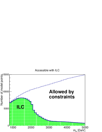
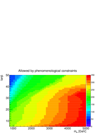
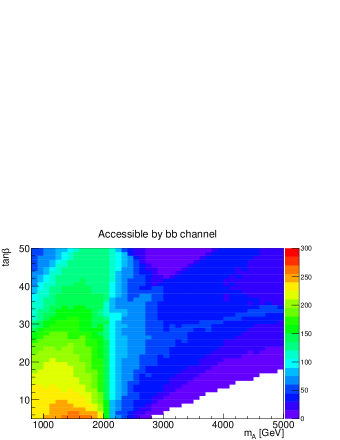
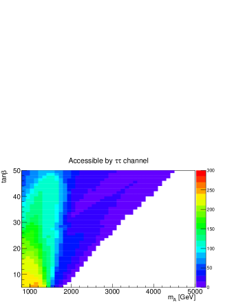
Figure 8: Upper-left: The number of model points accessible with ILC by at least one decay mode of $h$ as a function of $m_{A}$ (green histogram), as well as that of model points allowed by the phenomenological constraints (dotted histogram). Upper-right: The number of model points allowed by the phenomenological constraints on $m_{A}$ vs. $\tan\beta$ plane. Lower-left: The number of model points accessible with ILC by $h\rightarrow\bar{b}b$. Lower-right: The number of model points accessible with ILC by $h\rightarrow\bar{\tau}\tau$.

Finally, we show how large fraction of the parameter space can be covered by future $e^{+}e^{-}$ colliders. For this purpose, we define the $\delta\chi_{F}^{2}$ variable as

$$\delta\chi_{F}^{2}=\frac{\left[\Gamma(h\rightarrow F)-\Gamma^{\rm(SM)}(h\rightarrow F)\right]^{2}}{[\delta\Gamma(h\rightarrow F)]^{2}},$$ (3.3)

where $\delta\Gamma(h\rightarrow F)$ is the expected accuracies of the determinations of the Higgs partial decay widths at ILC with $\sqrt{s}=1\,{\rm TeV}$ and $\int\!dt\,\mathcal{L}=2500\,{\rm fb^{-1}}$ (see Table 1). Based on this quantity, we define the parameter region which is accessible with ILC at $\delta\chi_{F}^{2}\geq 4$. We perform a parameter scan and study if each model point is accessible with ILC and satisfies the phenomenological constraints. The MSSM parameters are scanned in the ranges of $800\,{\rm GeV}\leq m_{A}\leq 5\,{\rm TeV}$ (with the step size of $100\,{\rm GeV}$), $5\leq\tan\beta\leq 50$ (with the step size of $1$), and $0.5\leq|\mu|/m_{\tilde{U}}\leq 2$ (with the step size of $0.1$). Thus, for each set of $(m_{A},\tan\beta)$, 384 model points are studied, taking account of positive and negative values of $\mu$ as well as all four solutions of $A_{t}$. In addition, we adopt the relations $m_{\tilde{Q}}=M_{3}=m_{\tilde{U}}$, and $m_{\tilde{D}}=m_{\tilde{L}}=m_{\tilde{E}}=\max(m_{\tilde{U}},|\mu|)$. Concentrating on the parameter space where the LHC will have a difficulty in finding superparticles, $m_{\tilde{U}}$ is taken to be $3$, $4$, and $5\,{\rm TeV}$. In Fig. 8, the ILC coverage of the parameter space of our scan is displayed. In the upper-left panel, we show the distribution of the number of model points accessible with ILC by any of the decay modes of $h$ as a function of $m_{A}$. The green histogram is a distribution of the number of model points which satisfy $\delta\chi_{F}^{2}\geq 4$ and the phenomenological constraints, while the dotted one is that satisfying the phenomenological constraints without imposing $\delta\chi_{F}^{2}\geq 4$. We find that the number reduces drastically at $m_{A}\sim 2\,{\rm TeV}$. In the upper-right panel, we show the number of model points which survive the phenomenological constraints on $m_{A}$ vs. $\tan\beta$ plane. Here, $\delta\chi_{F}^{2}\geq 4$ is not imposed. Then, in the lower panels, we show the numbers of model points which can be accessed by the decay modes of $h\rightarrow\bar{b}b$ (lower-left) and $h\rightarrow\bar{\tau}\tau$ (lower-right) with taking account of the phenomenological constraints. They reduce significantly for $m_{A}\gtrsim 2\,{\rm TeV}$ irrespective of $\tan\beta$. The accessible points for $m_{A}\gtrsim 2\,{\rm TeV}$ are mostly with PL or NL solution.

4 Conclusions and Discussion

In this paper, we have studied the partial decay widths of the lightest Higgs boson in the MSSM. Taking account of relevant phenomenological constraints, i.e., Higgs mass, flavor constraints, vacuum stability, and the perturbativity of coupling constants up to the GUT scale, we have calculated the expected deviations of the partial decay widths from the SM predictions.

The partial decay widths are enhanced if the $\mu$-parameter is relatively large. However, such a choice may conflict with some of the phenomenological constraints. In particular, the vacuum-stability condition imposes a stringent constraint on the parameter space. We have found that, with too large $|\mu|$, there show up CCB vacua where the down-type Higgs field as well as the up-type Higgs and stop fields acquire large VEVs; existence of such CCB vacua was not seriously considered in the previous studies. In addition, when $\mu\tan\beta$ is large, non-holomorphic correction to the bottom Yukawa interaction becomes so large that the bottom Yukawa coupling constant becomes non-perturbative below the GUT scale. Large value of $\mu\tan\beta$ may also cause too large flavor-violating decay of $B$-mesons. By taking these constraints into account, the maximal and minimal possible values of the Higgs partial widths are restricted.

We found that the deviations of the partial decay widths from the SM predictions can be of $\mathcal{O}(1)$ % for some of the decay modes. In particular, those of $\Gamma(h\rightarrow\bar{b}b)$ and $\Gamma(h\rightarrow\bar{\tau}\tau)$ may show significant deviations even if the superparticles are out of the reach of 14TeV LHC. In addition, the deviation of $\Gamma(h\rightarrow gg)$ may also be sizable if the superparticles are relatively light. We emphasize that, although our scan is limited to some part of the MSSM parameter space, we have found the regions where the deviations from the SM predictions are within the reach of proposed $e^{+}e^{-}$ colliders even if superparticles would not be observed at the LHC.

Acknowledgements: The authors would like to thank Yasuhiro Shimizu for the collaboration in the early stage of this project. The authors also acknowledge YITP for their hospitality, at which this work was initiated. This work is supported by JSPS KAKENHI No. 23740172 (M.E.), No. 26400239 (T.M.), and No. 26287039 (M.M.N.). The work is supported by Grant-in-Aid for Scientific research from the Ministry of Education, Science, Sports, and Culture (MEXT), Japan, No. 23104008 (T.M.) and No. 23104006 (M.M.N.), and also by World Premier International Research Center Initiative (WPI Initiative), MEXT, Japan.

References

- [1] G. Aad et al. [ATLAS Collaboration], Phys. Lett. B 716 (2012) 1 [arXiv:1207.7214 [hep-ex]].
- [2] S. Chatrchyan et al. [CMS Collaboration], Phys. Lett. B 716 (2012) 30 [arXiv:1207.7235 [hep-ex]].
- [3] S. Dawson, A. Gritsan, H. Logan, J. Qian, C. Tully, R. Van Kooten, A. Ajaib and A. Anastassov et al., arXiv:1310.8361 [hep-ex].
- [4] Y. Okada, M. Yamaguchi and T. Yanagida, Prog. Theor. Phys. 85 (1991) 1.
- [5] Y. Okada, M. Yamaguchi and T. Yanagida, Phys. Lett. B 262, 54 (1991).
- [6] J. R. Ellis, G. Ridolfi and F. Zwirner, Phys. Lett. B 257 (1991) 83.
- [7] J. R. Ellis, G. Ridolfi and F. Zwirner, Phys. Lett. B 262, 477 (1991).
- [8] H. E. Haber and R. Hempfling, Phys. Rev. Lett. 66 (1991) 1815.
- [9] P. Z. Skands, B. C. Allanach, H. Baer, C. Balazs, G. Belanger, F. Boudjema, A. Djouadi and R. Godbole et al., JHEP 0407 (2004) 036 [hep-ph/0311123].
- [10] K. A. Olive et al. (Particle Data Group), Chin. Phys. C, 38, 090001 (2014).
- [11] S. Heinemeyer, W. Hollik and G. Weiglein, Comput. Phys. Commun. 124, 76 (2000) [hep-ph/9812320].
- [12] S. Heinemeyer, W. Hollik and G. Weiglein, Eur. Phys. J. C 9, 343 (1999) [hep-ph/9812472].
- [13] G. Degrassi, S. Heinemeyer, W. Hollik, P. Slavich and G. Weiglein, Eur. Phys. J. C 28, 133 (2003) [hep-ph/0212020].
- [14] M. Frank, T. Hahn, S. Heinemeyer, W. Hollik, H. Rzehak and G. Weiglein, JHEP 0702, 047 (2007) [hep-ph/0611326].
- [15] T. Hahn, S. Heinemeyer, W. Hollik, H. Rzehak and G. Weiglein, Phys. Rev. Lett. 112 (2014) 14, 141801 [arXiv:1312.4937 [hep-ph]].
- [16] L. J. Hall, R. Rattazzi and U. Sarid, Phys. Rev. D 50, 7048 (1994) [hep-ph/9306309, hep-ph/9306309].
- [17] R. Hempfling, Phys. Rev. D 49, 6168 (1994).
- [18] M. S. Carena, M. Olechowski, S. Pokorski and C. E. M. Wagner, Nucl. Phys. B 426, 269 (1994) [hep-ph/9402253].
- [19] M. S. Carena, S. Mrenna and C. E. M. Wagner, Phys. Rev. D 60, 075010 (1999) [hep-ph/9808312].
- [20] H. Eberl, K. Hidaka, S. Kraml, W. Majerotto and Y. Yamada, Phys. Rev. D 62, 055006 (2000) [hep-ph/9912463].
- [21] M. S. Carena, D. Garcia, U. Nierste and C. E. M. Wagner, Nucl. Phys. B 577, 88 (2000) [hep-ph/9912516].
- [22] L. Hofer, U. Nierste and D. Scherer, JHEP 0910, 081 (2009) [arXiv:0907.5408 [hep-ph]].
- [23] D. Noth and M. Spira, Phys. Rev. Lett. 101, 181801 (2008) [arXiv:0808.0087 [hep-ph]].
- [24] M. S. Carena, H. E. Haber, H. E. Logan and S. Mrenna, Phys. Rev. D 65 (2002) 055005 [Erratum-ibid. D 65 (2002) 099902] [hep-ph/0106116].
- [25] A. Arvanitaki and G. Villadoro, JHEP 1202, 144 (2012) [arXiv:1112.4835 [hep-ph]].
- [26] M. Reece, New J. Phys. 15, 043003 (2013) [arXiv:1208.1765 [hep-ph]].
- [27] E. Bagnaschi, R. V. Harlander, S. Liebler, H. Mantler, P. Slavich and A. Vicini, JHEP 1406, 167 (2014) [arXiv:1404.0327 [hep-ph]].
- [28] S. Heinemeyer, W. Hollik and G. Weiglein, Eur. Phys. J. C 16 (2000) 139 [hep-ph/0003022].
- [29] M. Cahill-Rowley, J. Hewett, A. Ismail and T. Rizzo, Phys. Rev. D 90 (2014) 9, 095017 [arXiv:1407.7021 [hep-ph]].
- [30] K. S. Babu and C. F. Kolda, Phys. Rev. Lett. 84, 228 (2000) [hep-ph/9909476].
- [31] S. R. Choudhury and N. Gaur, Phys. Lett. B 451, 86 (1999) [hep-ph/9810307].
- [32] G. Buchalla and A. J. Buras, Nucl. Phys. B 400, 225 (1993).
- [33] M. Misiak and J. Urban, Phys. Lett. B 451, 161 (1999) [hep-ph/9901278].
- [34] C. Bobeth, T. Ewerth, F. Kruger and J. Urban, Phys. Rev. D 64, 074014 (2001) [hep-ph/0104284].
- [35] C. Bobeth, A. J. Buras, F. Kruger and J. Urban, Nucl. Phys. B 630, 87 (2002) [hep-ph/0112305].
- [36] C. Bobeth, M. Gorbahn, T. Hermann, M. Misiak, E. Stamou and M. Steinhauser, Phys. Rev. Lett. 112 (2014) 101801 [arXiv:1311.0903 [hep-ph]].
- [37] V. Khachatryan et al. [CMS and LHCb Collaborations], arXiv:1411.4413 [hep-ex].
- [38] Y. Amhis et al. [Heavy Flavor Averaging Group (HFAG) Collaboration], arXiv:1412.7515 [hep-ex].
- [39] M. Misiak, H. M. Asatrian, K. Bieri, M. Czakon, A. Czarnecki, T. Ewerth, A. Ferroglia and P. Gambino et al., Phys. Rev. Lett. 98, 022002 (2007) [hep-ph/0609232].
- [40] F. Mahmoudi, Comput. Phys. Commun. 180 (2009) 1579 [arXiv:0808.3144 [hep-ph]].
- [41] W. Altmannshofer, M. Carena, N. R. Shah and F. Yu, JHEP 1301 (2013) 160 [arXiv:1211.1976 [hep-ph]].
- [42] J. M. Frere, D. R. T. Jones and S. Raby, Nucl. Phys. B 222, 11 (1983).
- [43] J. F. Gunion, H. E. Haber and M. Sher, Nucl. Phys. B 306, 1 (1988).
- [44] J. A. Casas, A. Lleyda and C. Munoz, Nucl. Phys. B 471, 3 (1996) [hep-ph/9507294].
- [45] A. Kusenko, P. Langacker and G. Segre, Phys. Rev. D 54, 5824 (1996) [hep-ph/9602414].
- [46] J. E. Camargo-Molina, B. O’Leary, W. Porod and F. Staub, JHEP 1312, 103 (2013) [arXiv:1309.7212 [hep-ph]].
- [47] D. Chowdhury, R. M. Godbole, K. A. Mohan and S. K. Vempati, JHEP 1402, 110 (2014) [arXiv:1310.1932 [hep-ph]].
- [48] N. Blinov and D. E. Morrissey, JHEP 1403, 106 (2014) [arXiv:1310.4174 [hep-ph]].
- [49] J. E. Camargo-Molina, B. Garbrecht, B. O’Leary, W. Porod and F. Staub, Phys. Lett. B 737, 156 (2014) [arXiv:1405.7376 [hep-ph]].
- [50] S. R. Coleman, Phys. Rev. D 15 (1977) 2929 [Erratum-ibid. D 16 (1977) 1248].
- [51] C. G. Callan, Jr. and S. R. Coleman, Phys. Rev. D 16 (1977) 1762.
- [52] C. L. Wainwright, Comput. Phys. Commun. 183 (2012) 2006 [arXiv:1109.4189 [hep-ph]].
- [53] K. E. Williams, H. Rzehak and G. Weiglein, Eur. Phys. J. C 71, 1669 (2011) [arXiv:1103.1335 [hep-ph]].
- [54] M. E. Peskin, arXiv:1312.4974 [hep-ph].