Nelson-Aalen tail product-limit process and extreme value index estimation under random censorship
Brahim Brahimi, Djamel Meraghni, Abdelhakim Necir∗
Laboratory of Applied Mathematics, Mohamed Khider University, Biskra, Algeria
Abstract
On the basis of Nelson-Aalen nonparametric estimator of the cumulative distribution function, we provide a weak approximation to tail product-limit process for randomly right-censored heavy-tailed data. In this context, a new consistent reduced-bias estimator of the extreme value index is introduced and its asymptotic normality is established only by assuming the second-order regular variation of the underlying distribution function. A simulation study shows that the newly proposed estimator performs better than the existing ones.
Keywords: Extreme values; Heavy tails; Hill estimator; Nelson-Aalen estimator; Random censoring; Tail index.
AMS 2010 Subject Classification: 62P05; 62H20; 91B26; 91B30.
Corresponding author:
necirabdelhakim@yahoo.fr
E-mail
addresses:
brah.brahim@gmail.com (B. Brahimi)
djmeraghni@yahoo.com (D. Meraghni)
1. Introduction
Let be independent copies of a non-negative random variable (rv) defined over some probability space with a cumulative distribution function (cdf) These rv’s are censored to the right by a sequence of independent copies of a non-negative rv independent of and having a cdf At each stage we can only observe the rv’s and with denoting the indicator function. The latter rv indicates whether there has been censorship or not. If we denote by the cdf of the observed then, by the independence of and we have Throughout the paper, we will use the notation for any Assume further that and are heavy-tailed or, in other words, that and are regularly varying at infinity with negative indices and respectively. That is
| (1.1) |
for any This class of distributions includes models such as Pareto, Burr, Fréchet, stable and log-gamma, known to be very appropriate for fitting large insurance claims, large fluctuations of prices, financial log-returns, … (see, e.g., Resnick, 2006). The regular variation of and implies that is regularly varying as well, with index where Since weak approximations of extreme value theory based statistics are achieved in the second-order framework (see de Haan and Stadtmüller, 1996), then it seems quite natural to suppose that cdf satisfies the well-known second-order condition of regular variation. That is, we assume that for any
| (1.2) |
where is the second-order parameter and is a function tending to not changing sign near infinity and having a regularly varying absolute value at infinity with index If interpret as In the sequel, the functions and respectively stand for the quantile and tail quantile functions of any given cdf The analysis of extreme values of randomly censored data, is a new research topic to which Reiss and Thomas (2007) made a very brief reference, in Section 6.1, as a first step but with no asymptotic results. Beirlant et al. (2007) proposed estimators for the extreme value index (EVI) and high quantiles and discussed their asymptotic properties, when the data are censored by a deterministic threshold. For their part, Einmahl et al. (2008) adapted various classical EVI estimators to the case where data are censored, by a random threshold, and proposed a unified method to establish their asymptotic normality. Their approach is used by Ndao et al. (2014, 2016) to address the nonparametric estimation of the conditional EVI and large quantiles. Based on Kaplan-Meier integration, Worms and Worms (2014) introduced two new estimators and proved their consistency. They showed, by simulation, that they perform better, in terms of bias and mean squared error (MSE) than the adapted Hill estimator of Einmahl et al. (2008), in the case where the tail index of the censored distribution is less than that of the censoring one. Brahimi et al. (2015) used the empirical process theory to approximate the adapted Hill estimator in terms of Gaussian processes, then they derived its asymptotic normality only under the usual second-order condition of regular variation. Their approach allows to relax the assumptions, made in Einmahl et al. (2008), on the heavy-tailed distribution functions and the sample fraction of upper order statistics used in estimate computation. Recently, Beirlant et al. (2016) developed improved estimators for the EVI and tail probabilities by reducing their biases which can be quite substantial. In this paper, we develop a new methodology, for the estimation of the tail index under random censorship, by considering the nonparametric estimator of cdf based on Nelson-Aalen estimator (Nelson, 1972; Aalen, 1976) of the cumulative hazard function
where A natural nonparametric estimator of is obtained by replacing and by their respective empirical counterparts and pertaining to the observed -sample. However, since we use instead of (see, e.g., Shorack and Wellner, 1986, page 295) to get
From the definition of we deduce that which by substituting for yields Nelson-Aalen estimator of cdf given by
where denote the order statistics, pertaining to the sample and the associated concomitants so that if Note that for our needs and in the spirit of what Efron (1967) did to Kaplan-Meier estimator (Kaplan and Meier, 1958) (given in we complete beyond the largest observation by In other words, we define a nonparametric estimator of cdf by
By considering samples of various sizes, Fleming and Harrington (1984) numerically compared with Kaplan-Meier (nonparametric maximum likelihood) estimator of (Kaplan and Meier, 1958), given in and pointed out that they are asymptotically equivalent and usually quite close to each other. A nice discussion on the tight relationship between the two estimators may be found in Huang and Strawderman (2006).
In the spirit of the tail product-limit process for randomly right-truncated data, recently introduced by Benchaira et al. (2016), we define Nelson-Aalen tail product-limit process by
| (1.3) |
where is an integer sequence satisfying suitable assumptions. In the case of complete data, the process reduces to where is the usual empirical cdf based on the fully observed sample Combining Theorems 2.4.8 and 5.1.4 in de Haan and Ferreira (2006), we infer that under the second-order condition of regular variation there exists a sequence of standard Weiner processes such that, for any and
| (1.4) |
where and One of the main applications of the this weak approximation is the asymptotic normality of tail indices. Indeed, let us consider Hill’s estimator (Hill, 1975)
which may be represented, as a functional of the process into
It follows, in view of approximation that
leading to provided that For more details on this matter, see for instance, de Haan and Ferreira (2006) page 76.
The major goal of this paper is to provide an analogous result to (1.4) in the random censoring setting through the tail product-limit process and propose a new asymptotically normal estimator of the tail index. To the best of our knowledge, this approach has not been considered yet in the extreme value theory literature. Our methodology is based on the uniform empirical process theory (Shorack and Wellner, 1986) and the related weak approximations (Csörgő et al., 1986). Our main result, given in Section 2 consists in the asymptotic representation of in terms of Weiner processes. As an application, we introduce, in Section 3, a Hill-type estimator for the tail index based on The asymptotic normality of the newly proposed estimator is established, in the same section, by means of the aforementioned Gaussian approximation of and its finite sample behavior is checked by simulation in Section 4. The proofs are postponed to Section 5 and some results that are instrumental to our needs are gathered in the Appendix.
2. Main result
Theorem 2.1.
Let and be two cdf’s with regularly varying tails (1.1) and assume that the second-order condition of regular variation (1.2) holds with Let be an integer sequence such that and where Then, there exists a sequence of standard Weiner processes defined on the probability space such that for every we have, as
| (2.5) |
where with
and
where and are two independent Weiner processes defined, for by
with
Remark 2.1.
It is noteworthy that the assumption is required to ensure that enough extreme data is available for the inference to be accurate. In other words, the proportion of the observed extreme values has to be greater than This assumption is already considered by Worms and Worms (2014) and, in the random truncation context, by Gardes and Stupfler (2015) and Benchaira et al. (2016).
Remark 2.2.
In the complete data case, we use instead of and we have This implies that and Since
it follows that and so approximations and agree for The symbol stands for equality in distribution.
3. Tail index estimation
In the last decade, some authors began to be attracted by the estimation of the EVI when the data are subject to random censoring. For instance, Einmahl et al. (2008) adapted the classical Hill estimator (amongst others) to a censored sample to introduce as an asymptotically normal estimator for where is Hill’s estimator of based on the complete sample and By using the empirical process theory tools and only by assuming the second-order condition of regular variation of the tails of and Brahimi et al. (2015) derived, in Theorem 2.1 (assertion a useful weak approximation to in terms of a sequence of Brownian bridges. They deduced in Corollary 2.1 that
| (3.6) |
provided that For their part, Worms and Worms (2014) proposed two estimators which incidentally can be derived, through a slight modification, from the one we will define later on. They proved their consistency (but not the asymptotic normality) by using similar assumptions as those of Einmahl et al. (2008). These estimators are defined by
and
where, for
| (3.7) |
are Kaplan-Meier estimators of and respectively. Thereafter, we will see that the assumptions under which we establish the asymptotic normality of our estimator are lighter and more familiar in the extreme value context. We start the definition of our estimator by noting that, from Theorem 1.2.2 in de Haan and Ferreira (2006), the first order condition of regular variation (1.1) implies that which, after an integration by parts, may be rewritten into
| (3.8) |
By replacing by and letting we obtain
| (3.9) |
as an estimator of Before we proceed with the construction of we need to define a function that is somewhat similar to and its empirical version by and respectively. Now, note that then we have
which may be rewritten into
which in turn simplifies to
By changing into and into with the necessary modifications, we end up with the following explicit formula for our new estimator of the EVI
where
| (3.10) |
Note that for uncensored data, we have and all the are equal to therefore for Indeed,
which leads to the formula of the famous Hill estimator of the EVI (Hill, 1975). The consistency and asymptotic normality of are established in the following theorem.
Theorem 3.1.
Let and be two cdf’s with regularly varying tails (1.1) such that Let be an integer sequence such that and then in probability, as Assume further that the second-order condition of regular variation (1.2) holds, then for all large
where and are those defined in Theorem 2.1. If in addition then
| (3.11) |
Remark 3.1.
We clearly see that, when there is no censoring the Gaussian approximation and the limiting distribution above perfectly agree with those of Hill’s estimator (see, e.g., de Haan and Ferreira, 2006, page 76).
Remark 3.2.
Since and then This implies that the absolute value of the asymptotic bias of is smaller than or equal to that of (see and In other words, the new estimator is of reduced bias compared to However, for any we have meaning that the asymptotic variance of is greater than that of This seems logical, because it is rare to reduce the asymptotic bias of an estimator without increasing its asymptotic variance. This is the price to pay, see for instance Peng (1998) and Beirlant et al. (2016). We also note that in the complete data case, both asymptotic biases coincide with that of Hill’s estimator and so do the variances.
4. Simulation study
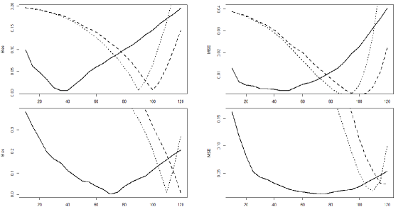
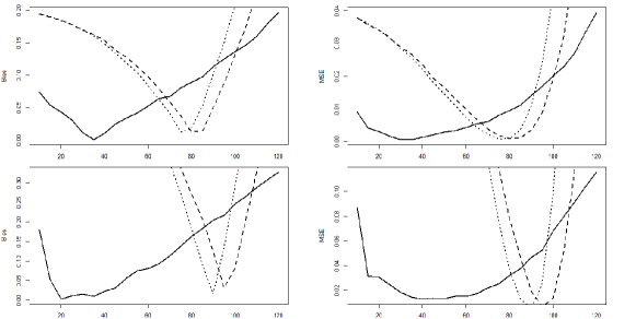
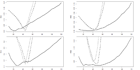
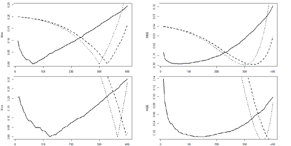
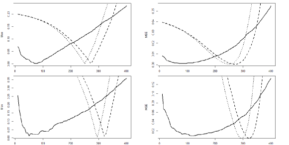
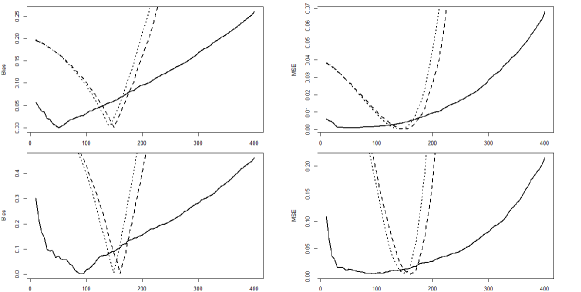
We mentioned in the introduction that Worms and Worms (2014) showed, by simulation, that their estimators outperform the adapted Hill estimator introduced by Einmahl et al. (2008). Therefore, this study is intended for comparing our estimator to and with respect to biases and MSE’s. It is carried out through two sets of censored and censoring data, both drawn from the following Burr models: and where We fix and choose the values and for For the proportion of really observed extreme values, we take and for strong, moderate and weak censoring respectively. For each couple we solve the equation to get the pertaining -value. We generate independent replicates of size then from both samples and Our overall results are taken as the empirical means of the results obtained through all repetitions. We plot the absolute biases and the MSE’s as functions of the number of upper order statistics used in the computation of the three estimators. The simulation results are illustrated, for the respective -values, in Figures 4.1, 4.2 and 4.3 for and in Figures 4.4, 4.5 and 4.6 for On the light of all the figures, it is clear that our estimator performs better than the other two. Indeed, in (almost) each case, the minima of the absolute bias and MSE of are less than those of and In addition, our estimator reaches its minima a long way before and do, meaning that the number of extremes needed for the last two estimators to be accurate is much larger than those needed for In other words, the cost of our estimator in terms of upper order statistics is very low compared to that of Worms and Worms estimators.
5. Proofs
In the sequel, we will use the following two empirical processes which may be represented, almost surely, by two uniform empirical ones. Indeed, let us consider the independent and identically distributed (iid) -uniform rv’s defined in (see Einmahl and Koning, 1992). The empirical cdf and the uniform empirical process based upon these rv’s are respectively denoted by
| (5.12) |
Deheuvels and Einmahl (1996) state that almost surely (a.s.)
| (5.13) |
for and It is easy to verify that a.s.
| (5.14) |
and
| (5.15) |
Our methodology strongly relies on the well-known Gaussian approximation, given by Csörgő et al. (1986) in Corollary 2.1. It says that on the probability space there exists a sequence of Brownian bridges such that, for every we have
| (5.16) |
For the increments we will need an approximation of the same type as Following similar arguments, mutatis mutandis, as those used in the proofs of assertions (2.2) of Theorem 2.1 and (2.8) of Theorem 2.2 in Csörgő et al. (1986), we may show that, for every we have
| (5.17) |
5.1. Proof of Theorem 2.1
The proof is carried out through two steps. First, we asymptotically represent is terms of the empirical cdf and the empirical sub-distributions functions and Second, we rewrite it as a functional of the following two processes
| (5.18) |
and
| (5.19) |
in order to apply the weak approximations and We begin, as in the proof of Theorem 2.1 in Benchaira et al. (2016), by decomposing into the sum of
and
In the following two subsections, we show that, uniformly on for any and small we have
| (5.20) |
where is the Gaussian process defined in Theorem 2.1. It is worth mentioning that both and may be rewritten in terms of Indeed, it is readily checked that
Then, we only focus on the weak approximation which will lead to that of and the asymptotic negligibility (in probability) of Finally, the approximation of will result in the asymptotic bias. In conclusion, we might say that representing amounts to representing
5.1.1. Representation of in terms of and
We show that, for all large and
| (5.21) |
where
and for every and small For notational simplicity, we write and without loss of generality, we attribute to any constant times and to any linear combinations of and for every We begin by letting which may be rewritten into whose empirical counterpart is equal to
Observe that then by replacing and by and respectively, we obtain Thus
| (5.22) |
By applying Taylor’s expansion, we may rewrite into
where is a stochastic intermediate value lying between and This allows us to decompose in into the sum of
and
First, we clearly see that Next, we show that and are approximations of and respectively, while as for any Since, from representation we have a.s., then without loss of generality, we may write
Let and set or, in other words, where denotes the empirical quantile function pertaining to By using this change of variables, we get
where, for notational simplicity, we set Now, we decompose into the sum of
and
It is clear that the change of variables yields that Hence, one has to show that as uniformly on We begin by for which an integration by parts gives
If denotes the interval of endpoints and then from Lemma we have uniformly on On the other hand, form representation we infer that
Then by using assertion in Proposition we have that
where and denote, the maximum and the minimum of and respectively. Observe that both and are regularly varying at infinity with the same index equal to Then by using assertion in Proposition we readily show that equals
Note that then it follows, after integration, that
which, by a change of variables, becomes
From now on, a key result related to the regular variation concept, namely Potter’s inequalities (see, e.g., Proposition B.1.9, assertion 5 in de Haan and Ferreira, 2006), will be applied quite frequently. For this reason, we need to recall this very useful tool here. Suppose that is a regularly varying function at infinity with index and let be positive real numbers. Then there exists such that for
| (5.23) |
Since and are regularly varying at infinity with respective indices and then we use to write that, for sufficiently small and for all large we have
From assertion of Lemma 4.1 in Brahimi et al. (2015), we have as hence On the other hand, we have and thus
Then, after integration, we obtain
We have therefore
By applying the mean value theorem, then assertion in Proposition we have
and by assertion in Proposition we get
Once again, by using the fact that together with routine manipulations of Potter’s inequalities we end up with Let us now consider the term which may be decomposed into the sum of
and
For the term we integrate the second integral by parts to get
| (5.24) |
Using assertion in Proposition 6.1 yields
which may be rewritten into
In the interval of endpoints and we have, for large is uniformly close to zero (in probability). On the other hand, assertion in Proposition implies that is uniformly stochastically bounded. Then, making use of Potter’s inequalities applied to the regularly varying function (with index we have
It is clear that
For the sake of simplicity, we rewrite this inequality into
which is in turn is less than of equal to In other words, we have
By making use of assertion in Proposition 6.1 (once again), we show that
Therefore
By a similar treatment as the above (we omit the details), we end up with For the term we start by noting that for any Since for it follows that
For the second integral, we use analogous arguments based on assertion in Proposition to write
Note that the latter integral is equal to By Potter’s inequalities on and the fact that it becomes By replacing by its expression, we get
Now, we apply Potter’s inequalities to to write
| (5.25) |
Since then and therefore
which, by (once again) using Potter’s inequalities to equals Then the right-hand side of is asymptotically equal to On the other hand, we have it follows that where is assumed to be greater than Consequently, we have for any and thus as well. By similar arguments, we show that asymptotically equals the same quantity, therefore we omit the details. Finally, we may write that For the term we proceed as we did for but with more tedious manipulations. By two steps, we have to get rid of integrands and and replace them by their theoretical counterparts and First, we define, for
By the change of variables and similar arguments to those used for the terms we show that
Second, we use the change of variables and proceed as above to get At this stage, we proved that is exactly and that and are approximated by and respectively. For the first remainder term it suffices to follow the same procedure to show that, uniformly on As for the last term we use similar technics to the decomposition
to show that as well, therefore we omit details. Now, the weak approximation of is well established.
5.1.2. Gaussian approximation to
We start by representing each in terms of the processes and Note that may be rewritten into
which, by integration by parts, becomes
Observe that, for and, from Lemma 4.1 in Brahimi et al. (2015), tends to as It follows that
Thus, after a change of variables, we have
Making the change of variables and using and yield
Next, we show that, for sufficiently small, we have
| (5.26) |
To this end, let us decompose into the sum of
We shall show that uniformly on while and are approximations to the first and second terms in respectively. Let us begin by and write
where Next, we provide a lower bound to by applying Potter’s inequalities to Since a.s., then from the right-hand side of we have a.s., which implies that a.s., for any as well. Let us now rewrite the sequence into
| (5.27) |
and use the left-hand side of Potter’s inequalities for the quantile function to get a.s., for any This implies that Then a.s. and therefore, from the left-hand side of (applied to we have a.s. uniformly on This allows us to write that
By combining Corollary 2.2.2 with Proposition B.1.10 in de Haan and Ferreira (2006), we have hence
From we infer that On the other hand, in view of assertion of Lemma 6.2, we have therefore
Note that then by using the right-hand side of (applied to we get
which equals Recall that then it is easy to verify that By using similar arguments, we also show that therefore we omit the details. For the term we have
In view of with the fact that we have
From assertion of Lemma 6.2, we have uniformly on then after elementary calculation, we end up with As for the first term it suffices to use Potter’s inequalities (for and to get
Finally, for we observe that which by a change of variables meets the second term in Let us now consider the term First, notice that
which, after an integration by parts, becomes
It follows that may be written into the sum of
and
For the first term, we replace and by and respectively and we get
By using the routine manipulations of Potter’s inequalities (applied to we obtain On the other hand, by the central limit theorem, we have as it follows that Since and then It is easy to verify that may be rewritten into
By using similar arguments as those used for we show that
therefore we omit the details. As for the third term we have
After a change of variables and an integration by parts in the first integral, we apply Potter’s inequalities to to show that
where
By using once again assertion in Proposition 6.1 with the fact that together with Potter’s inequalities routine manipulations, we readily show that uniformly on therefore we omit the details. Recall that and let us rewrite the first term in into
which, by an integration by parts, becomes
The first term above may be rewritten into and by similar arguments as those used for we show that the second term equals and thus we have
Consequently, we have
For the term routine manipulations lead to
where
By a similar treatment as that of we get By substituting the results obtained above, for the terms in equation we end up with
The asymptotic negligibility (in probability) of is readily obtained. Indeed, note that we have and from Theorem 2 in Csörgő (1996), we infer that This means that (because Recall now that
which, by applying Potter’s inequalities to yields that is equal to
Therefore
where
which, by routine manipulations as the above, is shown to be equal to
Therefore, we have
We are now in position to apply the well-known Gaussian approximation to get
where and are two Gaussian processes defined by
By similar arguments as those used in Lemma 5.2 in Brahimi et al. (2015), we end up with
where and are sequences of centred Gaussian processes defined by and Let be a sequence of Weiner processes defined on so that
| (5.28) |
It is easy to verify that which is exactly Finally, we take care of the term To this end, we apply the uniform inequality of second-order regularly varying functions to (see, e.g., the bottom of page 161 in de Haan and Ferreira (2006)), to write
and
uniformly on Since is regularly varying at infinity (with index and it follows that therefore
By assumption we have then
Let such that then
Now, we choose sufficiently small so that Since then hence for
uniformly on To achieve the proof it suffices to replace by and choose so that as sought.
5.2. Proof of Theorem 3.1
For the consistency of we make an integration by parts and a change of variables in equation to get
which may be decomposed into the sum of and By using the regular variation of and the corresponding Potter’s inequalities we get as Then, we just need to show that tends to zero in probability. From we have
where the second integral above is finite and therefore the second term of is negligible in probability. On the other hand, we have where and are the two centred Gaussian processes given in Theorem 2.1. After some elementary but tedious manipulations of integral calculus, we obtain
| (5.29) | |||
Since is a sequence Weiner processes, we may readily show that
But hence and thus it is easy to verify that This yields that when (because as sought. As for the Gaussian representation result, we write then by applying Theorem 2.1 together with the representation and the assumption, we have we get where
and The computation of the limit of gives
which by substituting for completes the proof.
Concluding notes
On the basis of Nelson-Aalen nonparametric estimator, we introduced a product-limit process for the tail of a heavy-tailed distribution of randomly right-censored data. The Gaussian approximation of this process proved to be a very useful tool in achieving the asymptotic normality of the estimators of tail indices and related statistics. Furthermore, we defined a Hill-type estimator for the extreme value index and determined its limiting Gaussian distribution. Intensive simulations show that the latter outperforms the already existing ones, with respect to bias and MSE. It is noteworthy that the asymptotic behavior of the newly proposed estimator is only assessed under the second-order condition of regular variation of the underlying distribution tail, in contrast to the unfamiliar assumptions of Worms and Worms (2014) and Einmahl et al. (2008). This represents the main big improvement brought in this paper. Our approach will have fruitful consequences and open interesting paths in the statistical analysis of extremes with incomplete data. The generalization of this approach to the whole range of maximum domains of attraction would make a very good topic for a future work.
6. Appendix
The following Proposition provides useful results with regards to the uniform empirical and quantile functions and respectively.
Proposition 6.1.
For and we have
For and we have
Let be a regularly varying function at infinity with index and let be such that and Then
Proof.
The proofs of assertion and the first result of assertion may be found in Shorack and Wellner (1986) in pages 415 (assertions 5-8 ) and 425 (assertion 16) respectively. The second result of assertion is proved by using the first results of both assertions and For the third assertion it suffices to apply Potter’s inequalities to function together with assertion corresponding to ∎
Lemma 6.1.
Let be the interval of endpoints and Then
where with being the generalized inverse of
Proof.
First, we show that, for any small there exists a constant such that is included in the half-open interval with probability close to as Indeed, following similar arguments as those used in the proof of part in Lemma 4.1 in Brahimi et al. (2015), we infer that for all large
| (6.30) |
uniformly on We have which implies that
Since and then
| (6.31) |
On the other hand, it is obvious that for any and a.s. Then, in view of assertion in Proposition we have it follows, from that uniformly on This means that there exists such that
| (6.32) |
Therefore, from and that tends to as for any where as sought. Next, let and It is clear that and that is for any Then, by using assertion of Proposition we get as uniformly on ∎
Lemma 6.2.
Let and be the two empirical processes respectively defined in and Then, for all large and any we have
Moreover, for any small we have uniformly on
where is of the form
Proof.
Recall that
and note that Then without loss of generality, we may write for any It is easy to verify that
Making use of Proposition 6.1 (assertion we infer that
uniformly on for any It follows that
On the other hand, by using Potter’s inequalities to both and with similar arguments as those used in the proof of Lemma 4.1 (assertion in Brahimi et al. (2015), we may readily show that Since then uniformly on We have and for any therefore uniformly on leading to the first result of assertion The proof of the second result follows similar arguments. For assertion we first note that
By using assertion we write uniformly on and by applying (once again) Potter’s inequalities to we infer that It follows that
which completes the proof. ∎
References
- Aalen (1976) Aalen, O., 1976. Nonparametric inference in connection with multiple decrement models. Scand. J. Statist. 3, 15-27.
- Beirlant et al. (2007) Beirlant, J., Guillou, A., Dierckx, G. and Fils-Villetard, A., 2007. Estimation of the extreme value index and extreme quantiles under random censoring. Extremes 10, 151-174.
- Beirlant et al. (2016) Beirlant, J., Bardoutsos, A., de Wet, T. and Gijbels, I., 2016. Bias reduced tail estimation for censored Pareto type distributions. Statist. Probab. Lett. 109, 78-88.
- Benchaira et al. (2016) Benchaira, S., Meraghni, D. and Necir, A. , 2016. Tail product-limit process for truncated data with application to extreme value index estimation. Extremes 19, 219-251.
- Bingham et al. (1987) Bingham, N.H., Goldie, C.M. and Teugels, J.L., 1987. Regular Variation. Cambridge University Press.
- Brahimi et al. (2015) Brahimi, B., Meraghni, D. and Necir, A., 2015. Approximations to the tail index estimator of a heavy-tailed distribution under random censoring and application. Math. Methods Statist. 24, 266-279.
- Csörgő et al. (1986) Csörgő, M., Csörgő, S., Horváth, L. and Mason, D.M., 1986. Weighted empirical and quantile processes. Ann. Probab. 14, 31-85.
- Csörgő (1996) Csörgő, S., 1996. Universal Gaussian approximations under random censorship. Ann. Statist. 24, 2744-2778.
- Deheuvels and Einmahl (1996) Deheuvels, P. and Einmahl, J.H.J., 1996. On the strong limiting behavior of local functionals of empirical processes based upon censored data. Ann. Probab. 24, 504-525.
- Efron (1967) Efron, B., 1967. The two-sample problem with censored data. Proceedings of the Fifth Berkeley Symposium on Mathematical Statistics 4, 831-552.
- Einmahl et al. (2008) Einmahl, J.H.J., Fils-Villetard, A. and Guillou, A., 2008. Statistics of extremes under random censoring. Bernoulli 14, 207-227.
- Einmahl and Koning (1992) Einmahl, J.H.J. and Koning, A.J., 1992. Limit theorems for a general weighted process under random censoring. Canad. J. Statist. 20, 77-89.
- Fleming and Harrington (1984) Fleming, T.R. and Harrington, D. P., 1984. Nonparametric estimation of the survival distribution in censored data. Comm. Statist. A-Theory Methods 13, 2469-2486.
- Gardes and Stupfler (2015) Gardes, L. and Stupfler, G., 2015. Estimating extreme quantiles under random truncation. TEST 24, 207-227.
- de Haan and Stadtmüller (1996) de Haan, L. and Stadtmüller, U., 1996. Generalized regular variation of second order. J. Australian Math. Soc. (Series A) 61, 381-395.
- de Haan and Ferreira (2006) de Haan, L. and Ferreira, A., 2006. Extreme Value Theory: An Introduction. Springer.
- Hill (1975) Hill, B.M., 1975. A simple general approach to inference about the tail of a distribution. Ann. Statist. 3, 1163-1174.
- Huang and Strawderman (2006) Huang, X. and Strawderman, R. L, 2006. A note on the Breslow survival estimator. J. Nonparametr. Stat. 18, 45-56.
- Kaplan and Meier (1958) Kaplan, E.L. and Meier, P., 1958. Nonparametric estimation from incomplete observations. J. Amer. Statist. Assoc. 53, 457-481.
- Ndao et al. (2014, 2016) Ndao, P., Diop, A. and Dupuy, J.-F., 2014. Nonparametric estimation of the conditional tail index and extreme quantiles under random censoring. Comput. Statist. Data Anal. 79, 63–79.
- Ndao et al. (2015) Ndao, P., Diop, A. and Dupuy, J.-F., 2016. Nonparametric estimation of the conditional extreme-value index with random covariates and censoring. J. Statist. Plann. Inference 168, 20-37.
- Nelson (1972) Nelson,W., 1972. Theory and applications of hazard plotting for censored failure data. Techno-metrics 14, 945-966.
- Peng (1998) Peng, L., 1998. Asymptotically unbiased estimators for the extreme-value index. Statist. Probab. Lett. 38, 107-115.
- Reiss and Thomas (2007) Reiss, R.-D. and Thomas, M., 2007. Statistical Analysis of Extreme Values with Applications to Insurance, Finance, Hydrology and Other Fields, 3rd ed. Birkhäuser Verlag, Basel, Boston, Berlin.
- Resnick (2006) Resnick, S., 2006. Heavy-Tail Phenomena: Probabilistic and Statistical Modeling. Springer.
- Shorack and Wellner (1986) Shorack, G.R. and Wellner, J.A., 1986. Empirical Processes with Applications to Statistics. Wiley.
- Worms and Worms (2014) Worms, J. and Worms, R., 2014. New estimators of the extreme value index under random right censoring, for heavy-tailed distributions. Extremes 17, 337-358.