Anisotropic spin motive force in multi-layered Dirac fermion system, $\alpha$-(BEDT-TTF)₂I₃

Abstract

We investigate the anisotropic spin motive force in $\alpha$-(BEDT-TTF)₂I₃, which is a multi-layered massless Dirac fermion system under pressure. Assuming the interlayer antiferromagnetic interaction and the interlayer anisotropic ferromagnetic interaction, we numerically examine the spin ordered state of the ground state using the steepest descent method. The anisotropic interaction leads to the anisotropic spin ordered state. We calculate the spin motive force produced by the anisotropic spin texture. The result quantitatively agrees with the experiment.

1 Introduction

An organic conductor $\alpha$-(BEDT-TTF)₂I₃ is a multi-layered massless Dirac fermion system, in which conduction layers of BEDT-TTF molecules and I₃ anions stack alternatively. In each conduction layers, the massless Dirac fermion system is realized. The valence band and the conduction band contact at two inequivalent points in the Brillouin zone. The energy dispersion is linear in the vicinity of the contact points. The Fermi energy coincides with the energy of the contact point. Therefore, the system is called Dirac fermion system.

Under the magnetic field $B$, the energy of the $n$-th Landau level of the Dirac fermion is described by $E={\rm sgn}(n)C\sqrt{|n|B}$ with a constant $C$. The energy difference between the first and the zeroth Landau levels is $C\sqrt{B}$. Therefore, in relatively high magnetic field, we may consider only the Landau level with $n=0$.

$\alpha$-(BEDT-TTF)₂I₃ has unique spin ordered states [1]. In each layer, the quantum Hall ferromagnetic state is realized by the intralayer ferromagnetic interaction due to the exchange interaction. On the other hand, the interlayer ferrimagnetic state is possible by the interlayer antiferromagnetic interaction.

($a$)

($b$)

Figure 1: The red arrow shows the interlayer tunneling direction. The BEDT-TTF molecules are described by the circles. $a$- and $b$-axis is in the conducting plane. $c$-axis is perpendicular to it. ($a$) The interlayer tunneling direction in $a$-$c$ plane. ($b$) The interlayer tunneling in $b$-$c$ plane is tilted in the direction to the $b$-axis.

$\alpha$-(BEDT-TTF)₂I₃ has anisotropic crystal structure and transport property. In figure 1, the direction of the interlayer tunneling is shown. The tunneling is tilted in the direction of $b$-axis. For the experimental data, the angle between the vertical direction and the interlayer tunneling direction is about $28^{\circ}$.

At low temperature and under magnetic field, anisotropic voltage is observed in $\alpha$-(BEDT-TTF)₂I₃ [2]. At high temperature the voltage disappears. The voltage increases with increasing the magnetic field. Therefore, one possible scenario is that the voltage is caused by spin motive force. The anisotropic crystal structure can lead to in the anisotropic voltage. The spin motive force produces the voltage. However, this is not a equilibrium situation. The spin motive force is transient due to the Gilbert damping. Charge accumulates at the edge of the system by the spin motive force and produces a electric field opposite to that created by spin motive force. The voltage will vanish due to the electric field created by the charge accumulation. Hereafter, for simplicity, we assume that the necessary time of the disappearance of the voltage is long and the voltage is constant in this time scale.

In this paper, we show that anisotropic spin ordered states are realized in $\alpha$-(BEDT-TTF)₂I₃ because of the interlayer anisotropic interaction and anisotropic spin motive forces are produced under magnetic field.

Figure 2: The anisotropic voltage in $\alpha$-(BEDT-TTF)₂I₃. The voltage in the direction of $a,b$ are defined by $V_{a},V_{b}$.

2 Model

We assume the square lattice for the conducting plane and the ferromagnetic interaction $J_{\rm intra}$ is assumed between nearest neighbor molecules. We define $b$- and $a$-axis as $x$- and $y$-axis, respectively. We take the direction of interlayer tunneling as $z$-axis. The interlayer interaction in the direction of tunneling is denoted by $J_{\rm inter}<0$. In this system, the lattice is distorted in $x$-$z$ plane since the molecular arrangement is tilted in the direction of $x$-axis and there are two different next nearest neighbor sites in $x$-$z$ plane. When the distance is different, the interaction should be different. For this reason, we assume a finite interaction $J^{\prime}_{\rm inter}$ in one of the next nearest neighbor sites in $x$-$z$ plane. On the other hand, for simplicity, we take a square lattice in $x$-$z$ plane in this calculation and assume the magnetic field is parallel to the $z$-axis.

($a$)	($b$)
($c$)	Figure 3: The model of $\alpha$-(BEDT-TTF)2I3. ($a$) Only $J_{\rm intra}$ exists in $x$-$y$ plane. ($b$) $J_{\rm inter}$ is along $z$-axis and $J_{\rm intra}$ is along $y$-axis in $y$-$z$ plane. ($c$) $J_{\rm inter}$ is along $z$-axis, $J_{\rm intra}$ is along $x$-axis and $J^{\prime}_{\rm inter}$ is between one side of the next nearest neighbor sites in $x$-$z$ plane.

The Hamiltonian under the magnetic field is written as

$$H = J_{{\rm intra}}\sum_{i,j,k}\left(\mathbf{S}_{i+1,j,k}+\mathbf{S}_{i,j+1,k}+\mathbf{S}_{i-1,j,k}+\mathbf{S}_{i,j-1,k}\right)\cdot\mathbf{S}_{i,j,k}$$ (1)

$$+ J_{{\rm inter}}\sum_{i,j,k}\left(\mathbf{S}_{i,j,k+1}+\mathbf{S}_{i,j,k-1}\right)\cdot\mathbf{S}_{i,j,k}+J^{\prime}_{{\rm inter}}\sum_{i,j,k}\left(\mathbf{S}_{i,j+1,k+1}+\mathbf{S}_{i,j-1,k-1}\right)\cdot\mathbf{S}_{i,j,k}$$

$$- \frac{1}{2}g\mu_{B}\sum_{i,j,k}\mathbf{B}\cdot\mathbf{S}_{i,j,k},$$

where $\mathbf{S}_{i,j,k}$ is a spin at the lattice point $(i,j,k)$. $g$ is g factor and $\mu_{B}$ is the Bohr magneton.

In this model, we investigate the spin ordered state of the ground state using the steepest descent method. At first, we put a spin with random direction on each lattice point. Next, we update spins with

$$\mathbf{n}_{i,j,k} = -\frac{J_{{\rm intra}}}{4}\left(\mathbf{n}_{i+1,j,k}+\mathbf{n}_{i,j+1,k}+\mathbf{n}_{i-1,j,k}+\mathbf{n}_{i,j-1,k}\right)$$

$$- \frac{J_{{\rm inter}}}{2}\left(\mathbf{n}_{i,j,k+1}+\mathbf{n}_{i,j,k-1}\right)-\frac{J^{\prime}_{{\rm inter}}}{2}\left(\mathbf{n}_{i,j+1,k+1}+\mathbf{n}_{i,j-1,k-1}\right)+\frac{1}{2}g\mu_{B}\mathbf{B}.$$

Here, $\mathbf{n}_{i,j,k}=2\mathbf{S}_{i,j,k}$ is the normalized localize moment. The resulting converged state is an approximate for the ground state. $J_{\rm intra}$ is proportional to the $\sqrt{B}$ [1], but, for simplicity, we assume $J_{\rm intra}$ is constant. We numerically calculate with the number of sites, $12\times 12\times 12$ and under the periodic boundary condition.

The result with the parameters $J_{\rm intra}=-5$ K, $J_{\rm inter}=4$ K, $J^{\prime}_{\rm inter}=-2$ K and $B=5$ T is shown in figure 4. Here, we assume relatively large value for $J_{\rm inter}$, which is the same order of magnitude as the interlayer hopping estimated in a related organic compound [3]. A ferromagnetic state is realized along $y$-axis. On the other hand, a periodic spin texture is created along $x$-axis due to the interlayer next nearest neighbor interaction.

($a$)

($b$)

Figure 4: The resulting spin ordered state of $\alpha$-(BEDT-TTF)₂I₃ with $J_{\rm intra}=-5$ K, $J_{\rm inter}=4$ K, $J^{\prime}_{\rm inter}=-2$ K and $B=5$ T. ($a$) The projection of spins in a layer to $x$-$y$ plane. A periodic spin ordered state is realized along $x$-axis, although a ferromagnetic structure is along $y$-axis. ($b$) The projection of spins in a layer to $x$-$z$ plane.

Assuming this spin ordered state, we calculate the spin motive force [4] in the strong coupling limit. In this limit, the spins are polarized and there are no conduction electron with minority spin. Therefore, the spin motive force is identical with the voltage. We make indices $j,k$ implicit below since we consider spin motive force in uniaxial direction. The localized moment is represented as

$$\begin{array}[]{ll}\mathbf{n}_{i}=(\cos\theta_{i}\cos\phi_{i},\cos\theta_{i}\sin\phi_{i},\sin\theta_{i}),\end{array}$$ (4)

where $\theta_{i}$ is the angle between the direction of the spin and the $z$-axis. $\phi_{i}$ is the angle between the direction of the spin projected in the $x$-$y$ plane and the positive direction of the $x$-axis. The electric field due to the localized moment is written as

$$\mathbf{E}_{i}=\frac{\hbar}{2e}\sin\theta_{i}\left[\left(\partial_{t}\theta_{i}\right)\left(\mathbf{\nabla}\phi_{i}\right)-\left(\partial_{t}\phi_{i}\right)\left(\mathbf{\nabla}\theta_{i}\right)\right],$$ (5)

where $e$ is the charge of the electron [5]. Here, the condition $\partial_{t}\theta_{i}=0$ and $\partial_{t}\phi_{i}=g\mu_{B}B/\hbar$ are always satisfied since the magnetic field is along $z$-axis. The electric field is rewritten as

$$\mathbf{E}_{i}=-\frac{g\mu_{B}}{2e}B\sin\theta_{i}\left(\mathbf{\nabla}\theta_{i}\right).$$ (6)

In the numerical calculation with the periodic boundary condition, the electric field is canceled if we take the average over the spatial period and so the spin motive force does not appear. However, in the real system, there is the edge of the sample and a finite spin motive force is possible. On the other hand, spin motive force along $y$-axis does not appear at all. Therefore, the spin motive force in this model has strong anisotropy. In order to estimate the spin motive force in the real system, we calculate the spin motive force with taking a part of the periodic spin structure.

The numerical result is shown in figure 5. The spin motive force along $x$-axis is on the order of $0.01$ mV to $0.1$ mV which is about the same order compared with the experimental result. The most of electric field is canceled and only the spin motive force in the vicinity of the edge remains. The experimental result shows that $V_{b}$ increases with increasing the magnetic field below $7$ T. In order to investigate the magnetic field dependence of $V_{b}$, we define the maximum value of the $V_{b}$ as $V_{\rm max}$. Although $V_{\rm max}$ does not always correspond to the experimental observed voltage, it is able to qualitatively evaluate the magnetic field dependence of $V_{b}$. The nurerical result of the magnetic field dependence of $V_{\rm max}$ is shown in figure 6. $V_{\rm max}$ increases with increasing magnetic field below $4$ T. However, above $5$ T, $V_{\rm max}$ decreases. Under high magnetic field, the Zeeman energy is larger than the intralayer and the interlayer interactions, and so $\{\theta_{i}\},\{\nabla\theta_{i}\}$ are small since we assume the interactions are constant. Therefore, the electric fields due to the localized moments vanish under high magnetic field. If we consider the magnetic field dependence of the interactions, we would evaluate the anisotropic spin motive force more precisely.

Figure 5: Spin motive forces along $x$-axis in $\alpha$-(BEDT-TTF)₂I₃. $n_{x}$ is the number of spins along $x$-axis from the edge of the system.

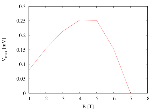
Figure 6: The magnetic field dependence of the maximum values of $V_{b}$. $V_{\rm max}$ increases with increasing magnetic field below 4 T and decreases above 5 T.

In a real system, the edge shape is different for a different layer. So, the naive expectation is that if we take the average over those edges, the spin motive force is canceled out. However, since the anisotropic spin motive force is generated by the three-dimensional structure, spins in regions without interlayer interaction should not contribute to the spin motive force. Therefore, it is justified to consider spin motive force for layers with the same edge shape.

3 conclusion

We have calculated the spin motive force in $\alpha$-(BEDT-TTF)₂I₃. The anisotropic interlayer interaction exists reflecting the anisotropic crystal structure. The anisotropic interaction leads to the unidirectional periodic spin structure. The anisotropic spin motive force is created from the anisotropic spin structure under magnetic field.

We would like to thank N. Tajima for discussions and sending us the experimental result. This work was financially supported in part by a Grant-in-Aid for Scientific Research (A) on “Dirac Electrons in Solids” (No. 24244053) and a Grant-in-Aid for Scientific Research (B) (No. 25287089) and (C) (No. 24540370) from the Ministry of Education, Culture, Sports, Science and Technology, Japan.

References

References

- [1] Kubo K and Morinari T 2014 J. Phys. Soc. Jpn. 83 033702
- [2] Tajima N Private communication
- [3] Jindo R, Sugawara S, Tajima N, Yamamoto M, Kato R, Nisino Y and Kajita K 2013 Phys. Rev. B 88 075315
- [4] Tatara G, Kohno H and Shibata J 2008 Physics Reports 468 213
- [5] Tserkovnyak Y and Mecklenburg M 2008 Phys. Rev. B 77 134407