Suzaku observations of the old pulsar wind nebula candidate HESS J1356$-$645

Abstract

A largely extended X-ray emission was discovered around the pulsar PSR J1357$-$6429 with the Suzaku deep observations. The pulsar, whose characteristic age is 7.3 kyr, is located within the TeV $\gamma$-ray source HESS J1356$-$645. The extended emission is found to have a 1$\sigma$ X-ray size of $\sim$4 arcmin, or $\sim$3 pc at 2.4 kpc, with a small offset from the pulsar. Its X-ray spectrum is well reproduced by a simple power-law model with a photon index of $1.70_{-0.06}^{+0.07}$. No significant spatial variation was found for the X-ray photon index as a function of distance from the pulsar. We conclude that the extended emission is associated to the pulsar wind nebula of PSR J1357$-$6429. This is a new sample of largely extended nebulae around middle-aged pulsars. We discuss the evolution of this PWN according to the relic PWN scenario.

1 Introduction

Pulsar wind nebulae (PWNe) consist of ultra-relativistic electrons and positrons accelerated by the pulsar termination shocks. Young PWNe are bright X-ray emitter via synchrotron process and are well studied in X-rays (Gaensler & Slane, 2006; Kargaltsev & Pavlov, 2008; Bamba et al., 2010b, for example). However, they become fainter in X-rays when the central pulsars get older (Mattana et al., 2009). Only limited studies exist for the older sources.

The atmospheric Cherenkov telescope for TeV (10¹² eV) gamma-rays, H.E.S.S. (High Energy Stereoscopic System), conducted Galactic plane survey since 2004 covering effectively the whole inner Galaxy, and discovered about fifty new sources in the very-high-energy (VHE) $\gamma$-ray band (Chaves & for the H. E. S. S. Collaboration, 2009). Because PWNe occupy the largest population of the identified Galactic VHE sources so far, majority of the new sources may also be the PWNe (Aharonian et al., 2006). A flow of high energy electrons and positrons in the PWNe contributes VHE $\gamma$-rays emission through inverse Compton scattering and X-rays through synchrotron emission. It became possible to estimate physical parameters of the PWNe, eg. magnetic field, by combining the VHE $\gamma$-ray and X-ray data. Thus the multi-wavelength studies of PWNe in VHE $\gamma$-rays and X-rays are very important to reveal their nature.

Recent studies of PWNe revealed the presence of extended X-ray emission with low surface brightness around the pulsar. Such emission may be produced by the ultra-relativistic electrons accelerated in the termination shocks. If so, its extension should correspond to the electron diffusion length during the energy-loss time scale. The energy-loss time scales of the X-ray emitting electrons may be 2–10 kyr assuming the magnetic field of the Galactic plane, 3–10 $\mu$G. This means that the electrons can travel $\sim$2 pc at the most. However, Suzaku observations showed that some PWNe had the extended emission with the size of more than 10 pc (Anada et al., 2010; Uchiyama et al., 2009). Furthermore, Bamba et al. (2010a) reported that the size of the extended emission from PWNe kept expanding up to $\sim$100 kyr in their characteristic ages. However, it is poorly understood how the emission region is formed and how it expands.

One of the key parameters to understand how the extend emission region is formed and evolves is the energy loss rate of the electrons. Because the ultra-relativistic electrons lose energy during diffusion, the non-thermal emission from the PWNe, which is well represented by a power-law, is expected to become softer with the distance from the pulsar. But this is sometimes not the case. Some PWNe showed no systematic variations in the photon indices of the power-law component with the distance from the pulsar (Anada et al., 2010; Uchiyama et al., 2009). This result may be explained if the ultra-relativistic electrons can diffuse with little loss of energy. However, it is not clear at present whether such lossless diffusion is plausible or not.

The pulsar PSR J1357$-$6429 ($P=166$ ms, $\dot{E}=3.1\times 10^{36}$ erg s^-1, surface magnetic field $B=7.8\times 10^{12}$ G) was discovered in the Parkes Multibeam Pulsar Survey (Camilo et al., 2004). The characteristic age, $\tau$, is 7.3 kyr. The distance of 2.4 kpc was estimated from the pulsar’s dispersion measure (DM $=127.2$ cm^-3 pc) and the Galactic free electron density model (Cordes & Lazio, 2002). PSR J1357$-$6429 is located within the TeV $\gamma$-ray source HESS J1356$-$645 (H.E.S.S. Collaboration et al., 2011). The extended TeV emission was detected up to 12’ from the peak of the TeV surface brightness, located at R.A. = 13h56m, dec. = -64D30’ (J2000). The TeV source was most likely powered by the pulsar because the separation of the center of the TeV source from the pulsar is only by $\sim$7’ and the TeV luminosity is $\sim 6\times 10^{33}$ erg s${}^{-1}~{}\sim 0.002\dot{E}$. At radio frequencies, Duncan et al. (1997) reported the extended emission from the supernova remnant (SNR) candidate G309.8$-$2.6, which is spatially coincident with HESS J1356$-$645. XMM-Newton and Chandra observed HESS J1356$-$645 in 2005 August for15 ks and in 2005 November for 33 ks, respectively. Zavlin (2007) and Esposito et al. (2007) reported that the pulsar spectrum likely consists of thermal and non-thermal components. Zavlin (2007) also reported a tail-like extended emission in the HRC-S image. Chang et al. (2012) suggested that this structure could be a pulsar jet or a part of the pulsar tail. Danilenko et al. (2012) found a possible optical counterpart of this pulsar and estimated the proper motion velocity to be $\sim$2000 km s^-1 to the north-eastern direction.

The X-ray Imaging Spectrometer (XIS; Koyama et al. (2007)) on board the Suzaku satellite (Mitsuda et al., 2007) has a low and stable background in contradiction to the limited sensitivity of XMM-Newton and Chandra for diffuse sources. Actually, Uchiyama et al. (2009) and Fujinaga et al. (2013) reported that the sizes of the extended emission around VHE gamma-ray sources determined by Suzaku were larger than the ones determined by XMM-Newton or Chandra. Therefore, XIS is ideal for observing faint and extended X-ray emission around HESS J1356$-$645. In addition, because it is located away from the Galactic plane, the observation would be less influenced by the Galactic Ridge X-ray Emission (GRXE). Thus, Suzaku observations would show new morphology of HESS J1356$-$645.

In this paper, we show the first Suzaku result on HESS J1356$-$645. In §2, we present the observation log and data reduction. Imaging and spectral analyses are shown in §3. We discuss the origin of the diffuse emission around PSR J1357$-$6429 in §4. Errors indicate single parameter 90% confidence regions throughout the paper.

2 Observations and Data Reduction

We observed the region around HESS J1356$-$645 with Suzaku in 2013 January and February. The observations were carried out with the two pointings in the east and west of HESS J1356$-$645 to cover the extended X-ray emission. The total exposures were 55.7 ks and 51.2 ks for the east and west region, respectively. Table 2 lists the journal of the Suzaku observations.

The Suzaku observations were performed with XIS in 0.3$-$10 keV and Hard X-ray Detector (HXD; Takahashi et al. (2007); Kokubun et al. (2007)) in 13$-$600 keV. XIS is located at the focal plane of the X-Ray Telescopes (XRT; Serlemitsos et al. (2007)), which provides a spatial resolution of $\sim\timeform{2^{\prime}}$ in a half-power diameter (HPD) and a field-of-view (FOV) of $\timeform{18^{\prime}}\times\timeform{18^{\prime}}$. The XIS system consists of one back-illuminated (BI) CCD camera (XIS1) and three front-illuminated (FI) CCDs (XIS0, 2, and 3). One of the front-illuminated CCDs, XIS2, was not usable at the time of our observations since it suffered from fatal damage on 2006 November 9. The XIS instruments were operated in the normal full-frame clocking mode (a frame time of 8 s) with Spaced-row Charge Injection (Nakajima et al., 2008). The HXD consists of silicon PIN photodiodes capable of observations in the 13$-$70 keV band and GSO crystal scintillators which cover the 40$-$600 keV band. Because we could not find any pulsations in the HXD data with good timing resolution of 61 $\mu$s (Terada et al., 2008), we focused on the XIS data analysis in this paper.

We used data sets processed by a set of software of the Suzaku data processing pipeline (version 2.5.16.29). The telemetry saturated time was excluded in the pipeline processing. Basic analysis was done using the HEASOFT software package (version 6.12). We used cleaned event files, in which standard screening was applied. The standard screening procedures include event grade selections, and removal of time periods such as spacecraft passage of the South Atlantic Anomaly, intervals of small geomagnetic cutoff rigidity, and those of a low elevation angle from the earth limb. Specifically, for the XIS, elevation angles larger than 5^∘ above the Earth and larger than 20^∘ from the sunlit Earth limb are selected.

*4c Journal of the observations Obs ID Observation date Aim point Effective exposure (ks)
507019010 2013/01/26$-$2013/01/28 (309.D99, -2.D55) 55.7
507020010 2013/02/17$-$2013/02/18 (309.D73, -2.D48) 51.3
In Galactic coordinates.

3 Analysis and Results

3.1 Background spectrum

Figure 1 shows XIS images of the region around HESS J1356$-$645 in the 0.5$-$2 keV and 2$-$8 kev bands. The Non X-ray background (NXB) generated by xisnxbgen (Tawa et al., 2008) was subtracted from the images. The images were binned by $8\times 8$ pixels and smoothed with a Gaussian function of $\sigma=2$ arcmin. We corrected the vignetting effect by dividing the image with a flat sky image, which was simulated using xissim (Ishisaki et al., 2007). In this simulation, we assumed the input energy spectrum as that extracted from the background region. We explain details of this background spectrum below.

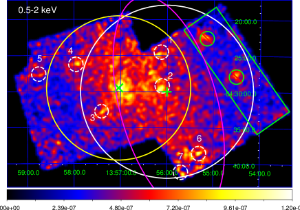
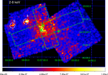
Figure 1: XIS image of the HESS J1356$-$645 field in the 0.5$-$2 keV (top) and the 2$-$8 keV (bottom) bands, respectively. These images were smoothed using a Gaussian function of $\sigma=2$ arcmin. The color scale is in units of counts s^-1/69.5 arcsec². A corner illuminated by the calibration source was removed. The peak position of the VHE $\gamma$-ray emission and PSR J1357$-$6429 is shown with $+$ and $\times$, respectively. The white and yellow circle (0.5$-$2 keV) indicates the extent of the VHE source (12’ in radius) and the region used for the spectral extraction (10’ in radius; see §3.3.1.), respectively. Note that the areas off the chip were not used in the analysis. The magenta ellipse marks the extent of the radio SNR candidate G309.8$-$2.6 (Parkes 2.4 GHz; Duncan et al. (1995)). The background region is shown with the green solid rectangle (5’.5$\times$18’). The sources 1$-$7 are catalogued by XMM-Newton. The diamond in the right panel indicate the peak position of the extended emission (see §3.2.1). The rectangles in the right panel are the regions for the profile analysis.

The background region (as depicted by the green solid rectangle in figure 1, which has an area of 91 arcmin²) was selected to minimize contamination from the diffuse emission. Two point-like sources not catalogued by XMM-Newton in the background region were removed with 1’ radius circular regions. After removing these point-like sources, we extracted the background spectrum. The background spectrum is shown in figure 2. There is no noticeable features of the emission lines in the background spectrum.

We fitted the background spectrum with the Cosmic X-ray Background (CXB) component and a power-law component for the remaining PWN emission. For the latter component, we do not have to distinguish whether the extended emission is stray light of central bright PWN or really extended and low surface brightness emission, since it does not change our result, as shown in section 3.2.1. We assumed the CXB as a power-law of photon index 1.4 with the intensity $5.4\times 10^{-15}$ erg s^-1 cm^-2 arcmin^-2 in the 2$-$10 keV band (Ueda et al., 1999). The hydrogen column density of the CXB was fixed to $0.84\times 10^{22}$ cm^-2 determined by HI observations (Kalberla et al., 2005). Note that the CXB emission has $\sim 10$% surface brightness fluctuation (Cappelluti et al., 2012), which is negligible compared with the background photons (see Figure 2). For the power-law component, the hydrogen column density, photon index, and normalization were set to be free parameters. The fitting was carried out for the FI and BI spectra simultaneously. The detector responses (RMF) and telescope responses (ARF) were generated by xisrmfgen and xissimarfgen (Ishisaki et al., 2007), respectively.

This model, however, was rejected with $\chi^{2}_{\mathrm{\nu}}=1.6$ (d.o.f.=225) with large residuals below 2 keV. We then added a thin thermal plasma component (APEC; Smith et al. (2001)) to this model, where metal abundances were fixed to the solar abundance while the other parameters were set free. The fit was improved to be $\chi^{2}_{\mathrm{\nu}}=1.4$ (d.o.f.=223), but still residuals were seen in the lower energy band. We then fitted the spectrum with two-temperature plasma and a power-law plus the CXB. The best-fit results are shown in table 1 and figure 2. The fit returned better $\chi^{2}_{\mathrm{\nu}}=1.3$ (d.o.f.=221), with no significant residuals. The low temperature component is consistent with the emission from the local hot bubble (Yoshino et al., 2009), whereas the high temperature one with the low-temperature component of the GRXE (Ryu et al., 2009). Note that such modeling is just for the reproduction of the background spectrum, thus we do not discuss separate components further.

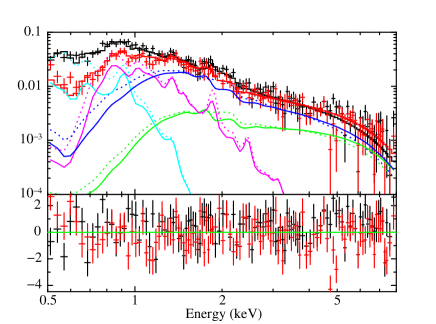
Figure 2: Energy spectra of the background region are displayed with the best-fit model. Red and Black crosses represent the FI and BI spectra, respectively. The best-fit models for FI and BI are plotted with dotted and solid lines, respectively. Individual components of the model are also shown for the thin thermal two-temperature plasma (cyan and magenta), a power-law (blue), and the CXB (green). Vertical error bars of each data point represent the 1$\sigma$ error.

Table 1: Best-fit parameters to the background spectrum.

	apec1	apec2	power-law	CXB
$kT$	$0.10^{+0.02}_{-0.01}$	$0.58^{+0.07}_{-0.12}$	-	-
$\Gamma$	-	-	$2.2^{+0.1}_{-0.1}$	(1.4)
Flux	27	2.2	2.4	(0.9)
NH	$0.53^{+0.10}_{-0.17}$			0.84
$\chi^{2}_{\nu}$(d.o.f.)	1.3(221)
Note: Values in the parenthesis are fixed in the fitting.
Plasma temperature [keV]
Photon index
Unabsorbed flux in the 0.5–10 keV band [$10^{-11}$ erg cm-2s-1]
Hydrogen column density [1022cm-2]

3.2 Image

In both the soft and hard band images, the position of the center of the brightest pixel is R.A.$=$13h57m01s.18, decl$=$-64D29’30”.4 (0.5$-$2 keV) and R.A.$=$13h56m59s.89, decl$=$-64D29’30”.4 (2$-$8 keV), respectively. The radio pulsar is located at R.A.$=$13h57m02s.43 (2), decl$=$-64D29’30”.2 (1) (Camilo et al., 2004). The difference of 8” ($0.5-2$ keV) and 16” ($2-8$ keV) between the X-ray and radio positions is smaller than the uncertainty in position of the XIS (19” at the 90$\%$ confidence level, Uchiyama et al. (2008)). Thus we concluded that the position of the brightest point-like source coincides with that of the radio pulsar.

An extended emission is clearly seen around PSR J1357$-$6429. Seven point-like sources in the soft band and two point-like sources in the hard band are identified in the XMM-Newton serendipitous source catalogue (3XMM). These point-like sources are summarized in table 3.2.

*3c Sources in the Suzaku fov from the XMM-Newton serendipitous source catalogue Source number Source name Source coordinate ($\mathrm{R.A._{J2000}},\mathrm{Decl._{J2000}}$)
1 $\mathrm{3XMM~{}J135607.6-642430}$ (209.0320, –64.4086)
2 $\mathrm{3XMM~{}J135704.4-642909}$ (209.2685, –64.4859)
3 $\mathrm{3XMM~{}J135724.4-643244}$ (209.3517, –64.5456)
4 $\mathrm{3XMM~{}J135757.2-642612}$ (209.4887, –64.4368)
5 $\mathrm{3XMM~{}J135845.3-642734}$ (209.6891, –64.4596)
6 $\mathrm{3XMM~{}J135518.7-643832}$ (208.8282, –64.6423)
7 $\mathrm{3XMM~{}J135541.9-644109}$ (208.9250, –64.6859)

3.2.1 Extended emission

In order to study the spatial distribution of the diffuse component, we made 1-dimensional profiles in the 2$-$8 keV band from the rectangular regions shown in figure 1 with the broken line. The regions were selected to be as wide as possible and to cross at right angles each other. The size of the region is 16’ $\times$ 5’ (region A) and 5’ $\times$ 28’ (region B), respectively. From Figure 1, one can see that the pulsar is not at the center of the diffuse emission. We set the center of the rectangular region not at the host pulsar but at the rough center of the diffuse emission, since our aim is to measure the extent of the diffuse emission. Figure 3 shows the 1-dimensional profiles of region A and B. We fitted the profiles with a model consisting of a Gaussian function (for the diffuse emission), a point spread function (PSF; for the pulsar) and a constant component (for the background). We approximated the PSF as a double Gaussian function, whose parameters (each width = 1.3’, 0.7’ and the intensity ratio = 2.3) were determined from the analysis of the 1-dimensional Suzaku image of the dwarf nova SS Cyg. The same data of SS Cyg were also used for the flight calibration of the PSF (Ishida et al., 2009). So, the fitting model is given by

$$y_{\mathrm{model}}=\mathrm{P_{0}}+\mathrm{P_{1}}\mathrm{exp}\left\{-\frac{1}{2}\left(\frac{x-\mathrm{P_{2}}}{\mathrm{P_{3}}}\right)^{2}\right\}$$

$$+\mathrm{P_{4}}\mathrm{exp}\left\{-\frac{1}{2}\left(\frac{x-\mathrm{P_{5}}}{1.3{\rm arcmin}}\right)^{2}\right\}$$

$$+2.3\mathrm{P_{4}}\mathrm{exp}\left\{-\frac{1}{2}\left(\frac{x-\mathrm{P_{5}}}{0.7{\rm arcmin}}\right)^{2}\right\}.$$ (1)

Here, $\mathrm{P_{0}}$, $\mathrm{P_{1}}$, and $\mathrm{P_{4}}$ are the intensity of background, diffuse, and point source (the pulsar), respectively, in the unit of $10^{-5}$counts s^-1, $\mathrm{P_{3}}$ is the extent of the diffuse emission in the unit of arcmin, and $\mathrm{P_{2}}$ and $\mathrm{P_{5}}$ is the offset of diffuse and point source from the arbitral origin in the unit of arcmin. In this method, we do not have to consider whether the remaining hard-tail emission in the background region is real low-surface brightness component or just due to stray light, since it does not change the width of the Gaussian fitting.

The fitting results are summarized in table 3. The fit gave the size of the diffuse emission ($P_{3}$) of 4’.1 $\pm$ 1’.4 (region A) and 4’.5 $\pm$ 0’.4 (region B), respectively. The center position of the diffuse emission was away from that of the pulsar by 1’.7 $\pm$ 0’.6 (region A) and 1’.3 $\pm$ 0’.3 (region B), respectively. The center of the diffuse emission is shown as a diamond in figure 1.

Figure 3: One-dimensional profiles of the diffuse emission. The solid lines represent the best-fit model consisting of a Gaussian, PSF and a constant function. The PSF is approximated by a double Gaussian (see text for details). The Gaussian and PSF are plotted as the broken lines. The bright peak in the region B (data points subtended by the two vertical dotted lines) corresponding to a point source was ignored in the fitting.

*8c Fitting results of the one-dimensional profiles Region P₀ P₁ P₂ P₃ P₄ P₅ $\chi^{2}$(d.o.f.)
[$10^{-5}$counts s^-1] [$10^{-5}$counts s^-1] [arcmin] [arcmin] [$10^{-5}$counts s^-1] [arcmin]
A $2.0\pm 1.1$ $3.2\pm 1.0$ $8.0\pm 0.3$ $4.1\pm 1.4$ $0.26\pm 0.16$ $9.7\pm 0.5$ 10.5(24)
B $1.5\pm 0.1$ $3.1\pm 0.2$ $13.2\pm 0.2$ $4.5\pm 0.4$ $0.60\pm 0.15$ $11.9\pm 0.2$ 26.2(43)

3.3 Energy spectrum

3.3.1 Source spectrum

In order to study the X-ray properties of the extended PWN, we need to exclude the emission from the central pulsar. However, it makes difficult to study the central part of PWN, due to the lack of spatial resolution of Suzaku. We thus first studied the energy spectrum of the total emission, sum of the pulsar and the diffuse emission, with the Suzaku data. We extracted the source spectrum from a 10’-radius circle depicted with the yellow circle in figure 1. As well as the image analysis, we removed the data of the point-like sources with a 1’-radius circle. We subtracted the background spectrum consisting of the NXB and the sky background emission discussed in §3.1. The NXB spectra were calculated using xisnxbgen. We compared the NXB and source spectra and found that the count rate of the calculated NXB is $\sim 83\%$ of that of the observed one above 10 keV, where NXB is the dominant component. It is considered the uncertainty of the NXB reproduction procedure (Mori et al., private communication), we adjusted the simulated NXB to fit the observed spectra above 10 keV. The sky background spectra were simulated using xspec by assuming the input energy spectrum extracted from the background region as shown in §3.1. The simulation was necessary to correctly incorporate the difference of the extraction regions and the energy dependent vignetting. This is the same method applied in Fujinaga et al. (2013). The exposure of the simulation was set to the same value as that of the Suzaku observations. The background subtracted spectrum is shown in figure 4.

The spectrum was fitted with an absorbed power-law model in the 0.5$-$10.0 keV band. The source region contains the pulsar. According to the spectral analysis of the Chandra observation (Chang et al., 2012), an emission from the pulsar itself was described with a thermal emission from the hydrogen atmosphere of a magnetized neutron star. Therefore, we added a NSA model to the above model. We adopted the NSA’s parameters from the Chandra observation, $T_{\mathrm{eff}}=0.96$ MK, $M_{\mathrm{ns}}=1.4\MO$, $R_{\mathrm{ns}}=10$ km, $B=$ 10¹³ G, and $D=$2.4 kpc. The fit was acceptable with a reduced $\chi^{2}$ of 221.6/253. The best-fit parameters are summarized in table 4. Note that the emission is more than one order of magnitude brighter than the power-law component in the background region, thus we can see that the source region cover the most part of the PWN emission.

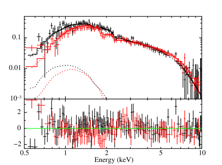
Figure 4: Energy spectrum of the source region. The best-fit model consisting of a power-law (solid) and NSA (dotted) is also shown. Black and red crosses show the BI and FI spectra, respectively. Vertical error bars of each data point represent a 1$\sigma$ error.

*4c Best-fit parameters of the spectrum in the source region. $N_{\mathrm{H}}$ $\Gamma$ $F_{\mathrm{unabs}}$ $\chi^{2}_{\nu}$(d.o.f.)
$0.35^{+0.05}_{-0.04}$ $1.70^{+0.07}_{-0.07}$ $7.9_{-0.3}^{+0.3}$ 0.88(253)
Column density [$10^{22}$cm^-2]
Photon index
Unabsorbed flux (2.0$-$10.0 keV) [$10^{-12}$erg s^-1 cm^-2]

3.3.2 Spatial variations of the spectrum

In order to investigate the spatial variations of the spectral shape, we divided the spectral extraction region into five annular ones, i.e., ”region 1” for the radius range of 0’$-$1’.5, ”region 2” for 1’.5$-$3’.5, ”region 3” for 3’.5$-$6’, ”region 4” for 6’$-$9’, and ”region 5” for 9’$-$12’. As well as the analysis of the source spectrum, the point-like sources were removed and the NXB and the sky background spectra were subtracted. We fitted each spectrum with an absorbed power-law model in the 0.5$-$10 keV band. In the fitting, we fixed the hydrogen column density at the average value, $N_{\mathrm{H}}=3.5\times 10^{21}$ cm^-2, determined by the spectrum analysis of entire emission in §3.3.1. to reduce the uncertainty due to limited statistics. For the region 1, we also added a fixed NSA component to reproduce the pulsar emission. The best-fit photon indices are shown in Figure 5 as a function of the distance from the pulsar. We can see that no significant spatial variation was detected in the photon indices.

Figure 5: Spatial variation of the photon indices from the pulsar PSR J1357$-$6429. No significant spatial variation was obtained.

4 Discussion

We have discovered an extended hard emission around the pulsar PSR J1357$-$6429. Because the emission has a power-law spectrum and is roughly centered at the pulsar, we consider that the emission is originated from the PWN associated to the pulsar. The emission size is $\sim$4 arcmin, or $\sim$3 pc at 2.4 kpc (Cordes & Lazio, 2002), which suggests that the PWN is one of the most extended samples among the young PWNe with the age of less than 10 kyr (Bamba et al., 2010a).

Bamba et al. (2010a) discussed that PWNe evolves up to the age of $\sim$100 kyr continuously expanding in size. The evolution may reflect the decay of magnetic field in PWNe and electrons can escape from the system before loosing their energy. The PWN of PSR J1357$-$6429 follows the relation between the age of the system (characteristic age of the pulsar) and the extent of the PWN suggested in Bamba et al. (2010a).

Relative positions of the center of the PWNe in different wavebands and the pulsar may be an important clue to understand the evolution of the PWNe. The center of the extended X-ray emission is found to be largely separated from the center of HESS J1356$-$645 in the TeV band, which coincide the radio center of the PWN (Duncan et al., 1995). The X-ray and TeV centers of the PWN are both offset from the pulsar, but the X-ray center is much closer to the pulsar than the TeV center (see Figure 1). The direction of the pulsar offset from the TeV center is similar to that of the proper motion of the pulsar (Danilenko et al., 2012). These facts may imply that the pulsar have traveled from the center of the TeV emission through the vicinity of X-ray center toward the current position. Such configuration of the PWN emission in each band and the pulsar may conform to the so-called relic PWN scenario (Blondin, Chevalier & Frierson, 2001; Aharonian et al., 2006; Kargaltsev & Pavlov, 2007). According to the scenario, the pulsar was born at the center of the TeV (and radio) emission with a supernova explosion 7.3 kyr ago, and reached the current position running toward the northeastern direction with the fast proper motion of $\sim$2000 km s^-1 (Danilenko et al., 2012). The pulsar accelerated electrons during the movement, which diffused out forming a PWN. When we consider the center position of the PWN, it is important to estimate the cooling times of energetic electrons. High energy electrons lose their energy quickly via the synchrotron emission, while less energetic electrons lose energy more slowly. Typical energy of X-ray emitting electrons, whose emission mechanism is via synchrotron process, may be $\sim$80 TeV for the assumed magnetic field of 10 $\mu$G (see eg. Bamba et al. (2010a)). On the other hand, the TeV gamma-ray emission may be produced by inverse Compton scattering of cosmic microwave background radiation by $\sim$10 TeV electrons. As a result, TeV emission sustains longer at the pulsar birthplace, whereas the X-ray emission is confined only nearby the present pulsar position. This means the X-ray emitting electrons are those accelerated recently.

The center of X-ray emission is offset from the pulsar by $\sim$2 arcmin. Because the X-ray center is calculated assuming a simple gaussian model and the direction of the offset is different from that of the proper motion of the pulsar, we consider that amount of the offset should be regarded just as a representative value. In spite of this ambiguity, we can still argue that the offset is much smaller than that of the TeV center ($\sim$7 arcmin). The X-ray offset is about one-third of the TeV offset. Assuming that the electrons emitting X-rays and TeV gamma-rays are accelerated around the pulsar and diffuse out in the same speed, and that electrons accelerated when the pulsar was very young still emit TeV gamma-rays, 7.3 kyrs ago (pulsar age), we can estimate the typical age of electrons emitting X-rays to be one-third of the pulsar age, very roughly, $\sim$2 kyr ago. Note that the pulsar spin-down age can differ by a factor 2–3 from true age, and the quantitative estimation of such numbers is very difficult.

This interpretation is also supported from the difference of the sizes of the emission regions. The extent of X-rays is $\sim$4 arcmin, which is again about one-third of the TeV extent of 0.2 degree again. This difference is naturally explained if the X-ray emitting electrons were accelerated recently.

We detected no significant spatial variations in the energy spectrum of the extended X-ray emission (Figure 5). This result cannot be interpreted in a simple way with the relic PWN scenario. The constant photon index means that the X-ray emitting electrons do not lose significant energy via synchrotron cooling during the diffusion from the pulsar, which conflicts with the offset of X-ray and TeV PWNe. This apparent conflict may be resolved if we introduce a sudden increase of acceleration efficiency when the reverse shock hit the PWN (Gelfand et al., 2009). Another possibility is that the acceleration efficiency became higher when the pulsar and dense interstellar matter collided to produce a strong bow-shock due to the fast proper motion of the pulsar. We need the magnetic field strength, configuration, and turbulence in order to estimate the diffusion time scale, which are beyond the scope of this paper, since all of these parameters are time-dependent (Bamba et al., 2010a). Further multi-wavelength studies of PWNe are needed.

We thank the anonymous referee for fruitful comments. M.I. and A.B. thank Makoto Sawada for his help on the Suzaku data analysis. We also thank Koji Mori for the useful comments on the NXB spectra. This work was supported in part by Grant-in-Aid for Scientific Research of the Japanese Ministry of Education, Culture, Sports, Science and Technology, No. 22684012 (A. B.).

References

- H.E.S.S. Collaboration et al. (2011) H.E.S.S. Collaboration, Abramowski, A., Acero, F., et al. 2011, A&A, 533, A103
- Aharonian et al. (2006) Aharonian, F., Akhperjanian, A. G., Bazer-Bachi, A. R., et al. 2006, ApJ, 636, 777
- Anada et al. (2010) Anada, T., Bamba, A., Ebisawa, K., & Dotani, T. 2010, PASJ, 62, 179
- Bamba et al. (2010a) Bamba, A., Anada, T., Dotani, T., et al. 2010a, ApJ, 719, L116
- Bamba et al. (2010b) Bamba, A., Mori, K., & Shibata, S. 2010b, ApJ, 709, 507
- Blondin, Chevalier & Frierson (2001) Blondin, J. M., Chevalier, R. A., & Frierson, D. M. 2001, ApJ, 563, 806
- Camilo et al. (2004) Camilo, F., Manchester, R. N., Lyne, A. G., et al. 2004, ApJ, 611, L25
- Cappelluti et al. (2012) Cappelluti, N., Ranalli, P., Roncarelli, M., et al. 2012, MNRAS, 427, 651
- Chang et al. (2012) Chang, C., Pavlov, G. G., Kargaltsev, O., & Shibanov, Y. A. 2012, ApJ, 744, 81
- Chaves & for the H. E. S. S. Collaboration (2009) Chaves, R. C. G., & for the H. E. S. S. Collaboration 2009, arXiv:0907.0768
- Cordes & Lazio (2002) Cordes, J. M., & Lazio, T. J. W. 2002, arXiv:astro-ph/0207156
- Danilenko et al. (2012) Danilenko, A., Kirichenko, A., Mennickent, R. E., et al. 2012, A&A, 540, A28
- Duncan et al. (1995) Duncan, A. R., Stewart, R. T., Haynes, R. F., & Jones, K. L. 1995, MNRAS, 277, 36
- Duncan et al. (1997) Duncan, A. R., Stewart, R. T., Haynes, R. F., & Jones, K. L. 1997, MNRAS, 287, 722
- Esposito et al. (2007) Esposito, P., Tiengo, A., de Luca, A., & Mattana, F. 2007, A&A, 467, L45
- Fujinaga et al. (2013) Fujinaga, T., Mori, K., Bamba, A., et al. 2013, PASJ, 65, 61
- Gaensler & Slane (2006) Gaensler, B. M., & Slane, P. O. 2006, Ann. Rev. Astron. Astrophys., 44, 17
- Gelfand et al. (2009) Gelfand, J. D., Slane, P. O., & Zhang, W. 2009, ApJ, 703, 2051
- Ishida et al. (2009) Ishida, M., Okada, S., Hayashi, T., et al. 2009, PASJ, 61, 77
- Ishisaki et al. (2007) Ishisaki, Y., Maeda, Y., Fujimoto, R., et al. 2007, PASJ, 59, 113
- Kalberla et al. (2005) Kalberla, P. M. W., Burton, W. B., Hartmann, D., et al. 2005, A&A, 440, 775
- Kargaltsev & Pavlov (2007) Kargaltsev, O & Pavlov, G. G. 2007, ApJ, 670, 655
- Kargaltsev & Pavlov (2008) Kargaltsev, O., & Pavlov, G. G. 2008, 40 Years of Pulsars: Millisecond Pulsars, Magnetars and More, 983, 171
- Kokubun et al. (2007) Kokubun, M., Makishima, K., Takahashi, T., et al. 2007, PASJ, 59, 53
- Koyama et al. (2007) Koyama, K., Tsunemi, H., Dotani, T., et al. 2007, PASJ, 59, 23
- Mattana et al. (2009) Mattana, F., Falanga, M., Götz, D., et al. 2009, ApJ, 694, 12
- Mitsuda et al. (2007) Mitsuda, K., Bautz, M., Inoue, H., et al. 2007, PASJ, 59, 1
- Nakajima et al. (2008) Nakajima, H., Yamaguchi, H., Matsumoto, H., et al. 2008, PASJ, 60, 1
- Rho & Petre (1998) Rho, J., & Petre, R. 1998, ApJ, 503, L167
- Ryu et al. (2009) Ryu, S. G., Koyama, K., Nobukawa, M., Fukuoka, R., & Tsuru, T. G. 2009, PASJ, 61, 751
- Serlemitsos et al. (2007) Serlemitsos, P. J., Soong, Y., Chan, K.-W., et al. 2007, PASJ, 59, 9
- Smith et al. (2001) Smith, R. K., Brickhouse, N. S., Liedahl, D. A., & Raymond, J. C. 2001, ApJ, 556, L91
- Takahashi et al. (2007) Takahashi, T., Abe, K., Endo, M., et al. 2007, PASJ, 59, 35
- Tawa et al. (2008) Tawa, N., Hayashida, K., Nagai, M., et al. 2008, PASJ, 60, 11
- Terada et al. (2008) Terada, Y., Enoto, T., Miyawaki, R., et al. 2008, PASJ, 60, 25
- Uchiyama et al. (2008) Uchiyama, Y., Maeda, Y., Ebara, M., et al. 2008, PASJ, 60, 35
- Uchiyama et al. (2009) Uchiyama, H., Matsumoto, H., Tsuru, T. G., Koyama, K., & Bamba, A. 2009, PASJ, 61, 189
- Ueda et al. (1999) Ueda, Y., Takahashi, T., Inoue, H., et al. 1999, ApJ, 518, 656
- Yoshino et al. (2009) Yoshino, T., Mitsuda, K., Yamasaki, N. Y., et al. 2009, PASJ, 61, 805
- Zavlin (2007) Zavlin, V. 2007, The Neutron Star Crust and Surface, Published online at http://www.astroscu.unam.mx/neutrones/INT/Workshop.html, p2