Soliton-induced Majorana fermions in a one-dimensional atomic topological superfluid

Abstract

We theoretically investigate the behavior of dark solitons in a one-dimensional spin-orbit coupled atomic Fermi gas in harmonic traps, by solving self-consistently the Bogoliubov-de Gennes equations. The dark soliton - to be created by phase-imprinting in future experiments - is characterized by a real order parameter, which changes sign at a point node and hosts localized Andreev bound states near the node. By considering both cases of a single soliton and of multiple solitons, we find that the energy of these bound states decreases to zero, when the system is tuned to enter the topological superfluid phase by increasing an external Zeeman field. As a result, two Majorana fermions emerge in the vicinity of each soliton, in addition to the well-known Majorana fermions at the trap edges associated with the nontrivial topology of the superfluid. We propose that the soliton-induced Majorana fermions can be directly observed by using spatially-resolved radio-frequency spectroscopy or indirectly probed by measuring the density profile at the point node. For the latter, the deep minimum in the density profile will disappear due to the occupation of the soliton-induced zero-energy Majorana fermion modes. Our prediction could be tested in a resonantly-interacting spin-orbit coupled ⁴⁰K Fermi gas confined in a two-dimensional optical lattice.

I Introduction

Solitonic excitations in quantum superfluids are of significant importance. They behave like quantum mechanical matter waves and maintain their shape during propagation. As highly nonlinear and localized topological excitations, solitons provide a very sensitive probe of the fundamental coherence properties of the underlying superfluid state in which they propagate. In the ultracold matter of weakly interacting Bose-Einstein condensates (BECs), where the phase coherence is associated with long-range order in the one-body density matrix, solitons have been investigated extensively over the past decade, both theoretically and experimentally Frantzeskakis2010 . In a series of ground-breaking experiments Burger1999 ; Denschlag2000 , dark solitons - appearing as a suppression in the density profile - have been created via phase-imprinting. Their theoretical description is provided by the nonlinear Gross-Pitaevskii equation Frantzeskakis2010 .

In strongly interacting fermionic superfluids, solitions are more interesting, as the phase coherence between the underlying bosonic entities (i.e., Cooper pairs), characterized by long-range order in the two-body density matrix, is more subtle to understand and describe Dziarmaga2005 ; Antezza2007 ; Liao2011 ; Scott2011 ; Spuntarelli2011 ; Cetoli2013 . In addition, fermionic bound states may be induced near solitonic defects Antezza2007 , analogous to the famous Andreev bound states inside vortex cores Caroli1964 . In this respect, the recent experimental realization of dark solitons in strongly-interacting atomic ⁶Li Fermi gases at the crossover from BECs to Bardeen-Cooper-Schrieffer (BCS) superfluids is of great interest Yefsah2013 . A fermionic soliton was nucleated in a controlled way by using the phase imprinting method in a cigar-shaped Fermi cloud and was observed as a reduced density slit running through the middle of the cloud. The soliton exhibited the expected oscillation when it moved from one end of the trap to the other. However, the rate of oscillation was much slower than that predicted from time-dependent mean-field calculations Liao2011 ; Scott2011 ; Spuntarelli2011 ; Cetoli2013 . This discrepancy is now solved by a refined measurement Ku2014 . Due to the intrinsic snake instability in three dimensions, the observed defect is actually the decay product of soliton. In the constrained geometry of the cloud, it is a single straight vortex line and therefore is better named as a solitonic vortex Ku2014 .

In this work, we consider the observation of dark solitons in an even more intriguing situation - topological fermionic superfluids Qi2011 . Our research is motivated by the recent opened perspective that atomic topological superfluids might be realized very soon in cold-atom laboratories with spin-orbit coupled Fermi gases of ⁴⁰K or ⁶Li atoms Wang2012 ; Cheuk2012 ; Williams2013 . Topological superfluids are novel states of matter, which have attracted considerable attention because of their non-trivial topological properties and their ability to host exotic quasi-particles known as Majorana fermions - particles that are their own anti-particles Majorana1937 ; Wilczek2009 . It is therefore of great interest to ask: will there be any interesting features exhibited by a superfluid when its topological order and a solitonic defect come into play?

To address this problem, we theoretically investigate the existence of dark solitons in a one-dimensional (1D) spin-orbit coupled atomic Fermi gas in a harmonic trap under an external Zeeman field. A dark soliton is characterized by a phase jump of $180^{\circ}$ at a point node at which the order parameter changes sign and crosses zero. As the number of dark solitons can be controlled by changing the number of phase jumps, we consider both cases of a single soliton and multiple solitons (i.e., a soliton train). In the topological superfluid phase, we find that each dark soliton is able to host two Majorana fermions, well localized around nodal point of the soliton. Potentially, this may provide an ideal scenario to create and move Majorana fermions towards realistic applications, via the control of phase-imprinting. We propose that experimentally the existence of dark solitons may be probed by using radio-frequency spectroscopy for the local density of state or absorption imaging for the density profile.

It should be noted that a dark soliton in one dimension behaves very similarly to a vortex in two dimensions. The latter is also a topological defect that can host a Majorana fermion in the vortex core and exhibit it in the local density of state and density profile Liu2012a . A vortex lattice in topological superfluids has been proposed to be an appealing platform to perform topological quantum information processing and quantum computation Nayak2008 ; Ivanov2001 . In principle, a soliton train would achieve a similar goal. A detailed discussion of this possibility will be addressed in a future publication.

We also note that recently Xu et al. investigated the properties of a single soliton in a 1D spin-orbit coupled Fermi gas Xu2014 . These authors considered a different set of parameters, with which the Fermi cloud enters a partial topological superfluid phase by increasing the external Zeeman field. Our results are in qualitative agreement with theirs when there are overlaps.

Our paper is arranged as follows. In the next section (Sec. II), we briefly introduce the model Hamiltonian and explain how to solve it in the mean-field picture of the Bogoliubov-de Gennes (BdG) equations, and then specify the parameter space (i.e., phase diagram) for our numerical results. In Sec. III, we study the properties of a single soliton and show the emergence of zero-energy Majorana fermions when the topological regime is approached. The wavefunctions of the Majorana fermions and their manifestations in the local density of state and density profile are discussed in detail. In Sec. IV, the cases of two and more solitons are considered. Finally, Sec. V is devoted to summaries and conclusions.

II Model Hamiltonian and mean-field theory

We consider a spin-1/2 ⁴⁰K Fermi gas of $N$ atoms with spin-orbit coupling confined in a 1D harmonic trap Liu2012b ; Wei2012 ; Liu2013 ; Jiang2014 . This system could be realized at Shanxi University, by adding a very deep 2D optical lattice (in the transverse $y$-$z$ plane) to a spin-orbit coupled 3D Fermi gas formed by two counter-propagating Raman laser beams (along the $x$-direction) Wang2012 . It can be described by a single-channel model Hamiltonian $H=\int dx[\mathcal{\mathscr{H}}_{0}+\mathcal{\mathscr{H}}_{int}$], where

$$\mathscr{H}_{0}=\sum_{\sigma=\uparrow,\downarrow}\Psi_{\sigma}^{\dagger}\mathcal{H}_{S}\Psi_{\sigma}-\frac{\Omega_{R}}{2}\left[\Psi_{\uparrow}^{\dagger}e^{i2k_{R}x}\Psi_{\downarrow}+\text{H.c.}\right]$$ (1)

is the single-particle part and

$$\mathscr{H}_{int}=g_{1D}\Psi_{\uparrow}^{\dagger}\left(x\right)\Psi_{\downarrow}^{\dagger}\left(x\right)\Psi_{\downarrow}\left(x\right)\Psi_{\uparrow}\left(x\right)$$ (2)

is the part describing the contact interaction between the two spin states. Here, $\sigma=\uparrow,\downarrow$ is the pseudo-spin denoting the two hyperfine states and $\Psi_{\sigma}^{\dagger}\left(x\right)$ is the fermionic field operator that creates an atom with mass $m$ in the spin state $\sigma$. The second term in $\mathscr{H}_{0}$ describes a synthetic spin-orbit coupling, where $\Omega_{R}$ and $k_{R}$ are the Rabi frequency and the wavevector of the laser beams, respectively. Due to the counter-propagating configuration, the momentum transferred during the two-photon Raman process is $2\hbar k_{R}$. The Hamiltonian

$$\mathcal{H}_{S}=-\frac{\hbar^{2}}{2m}\frac{\partial^{2}}{\partial x^{2}}-\mu+V_{T}(x),$$ (3)

with $\mu$ being the chemical potential and $V_{T}\left(x\right)\equiv m\omega^{2}x^{2}/2$ the 1D harmonic trapping potential with an oscillation frequency $\omega$. The motion of atoms in the $y$-$z$ plane is frozen due to the tight 2D optical lattice (i.e., the transverse trapping frequency $\omega_{\perp}\sim N\omega\gg\omega$). In this quasi-1D geometry, it is known that the low-energy scattering properties of atoms can be well described using a contact potential $g_{1D}\delta(x)$, where the 1D effective coupling constant $g_{1D}<0$ can be expressed through the 3D scattering length $a_{3D}$ Bergeman2003 ,

$$g_{1D}=\frac{2\hbar^{2}a_{3D}}{ma_{\perp}^{2}}\frac{1}{\left(1-{\cal A}a_{3D}/a_{\perp}\right)},$$ (4)

where $a_{\perp}\equiv\sqrt{\hbar/(m\omega_{\perp})}$ and the constant ${\cal A}=-\zeta(1/2)/\sqrt{2}\simeq 1.0326$. The interatomic interaction of our trapped system can be conveniently parameterized by a dimensionless interaction parameter Hu2007a ; Liu2007 ; Liu2008

$$\gamma\equiv-\frac{mg_{1D}}{\hbar^{2}n_{0}},$$ (5)

which is basically the ratio between the mean-field interaction energy and the kinetic energy. Here $n_{0}=(2/\pi)\sqrt{Nm\omega/\hbar}$ is the total atomic density of a non-interacting Fermi gas at the trap center within the local density approximation. Experimentally, in the vicinity of Feshbach resonances (i.e., $a_{3D}\rightarrow\pm\infty$), the typical value of the interaction parameter $\gamma$ is about $5$ Liao2010 .

To solve the single-channel model Hamiltonian $H$, it is useful to apply a local gauge transformation Liu2012b ; Wei2012 ; Jiang2014 ,

$$\Psi_{\uparrow}\left(x\right) = e^{+ik_{R}x}\frac{1}{\sqrt{2}}\left[\psi_{\uparrow}\left(x\right)-i\psi_{\downarrow}\left(x\right)\right],$$ (6)

$$\Psi_{\downarrow}\left(x\right) = e^{-ik_{R}x}\frac{1}{\sqrt{2}}\left[\psi_{\uparrow}\left(x\right)+i\psi_{\downarrow}\left(x\right)\right].$$ (7)

Using the new field operators $\psi_{\uparrow}\left(x\right)$ and $\psi_{\downarrow}\left(x\right)$, we can recast the single-particle Hamiltonian into the form,

$$\mathscr{H}_{0} = \left[\psi_{\uparrow}^{\dagger}\left(x\right),\psi_{\downarrow}^{\dagger}\left(x\right)\right]{\cal H}_{0}\left[\begin{array}[]{c}\psi_{\uparrow}\left(x\right)\\ \psi_{\downarrow}\left(x\right)\end{array}\right],$$ (10)

$${\cal\mathcal{H}}_{0} = -\frac{\hbar^{2}}{2m}\frac{\partial^{2}}{\partial x^{2}}+V_{T}\left(x\right)-\mu-h\sigma_{z}+\lambda\hat{k}_{x}\sigma_{y},$$ (11)

where we have redefined the chemical potential $\mu\rightarrow\mu-\hbar^{2}k_{R}^{2}/(2m)$ to absorb a constant energy shift and have introduced the momentum operator $\hat{k}_{x}\equiv-i\partial/\partial x$, the spin-orbit coupling constant $\lambda\equiv\hbar^{2}k_{R}/m$ and an effective Zeeman field $h\equiv\Omega_{R}/2$. Furthermore, $\sigma_{y}$ and $\sigma_{z}$ are Pauli matrices. The form of the interaction Hamiltonian is invariant under the local gauge transformation, i.e.,

$$\mathscr{H}_{int}=g_{1D}\psi_{\uparrow}^{\dagger}\left(x\right)\psi_{\downarrow}^{\dagger}\left(x\right)\psi_{\downarrow}\left(x\right)\psi_{\uparrow}\left(x\right).$$ (12)

The operator for the total atomic density $\hat{n}(x)\equiv\sum_{\sigma}\Psi_{\sigma}^{\dagger}\left(x\right)\Psi_{\sigma}\left(x\right)=\sum_{\sigma}\psi_{\sigma}^{\dagger}\left(x\right)\psi_{\sigma}\left(x\right)$ is also invariant. However, the form of the density operator for each spin component changes Wei2012 .

II.1 Bogoliubov-de Gennes equations

We solve the single-channel model Hamiltonian within the standard mean-field framework. By introducing an order parameter $\Delta\left(x\right)\equiv-g_{1D}\left\langle\psi_{\downarrow}\left(x\right)\psi_{\uparrow}\left(x\right)\right\rangle$, the interaction Hamiltonian can be approximated as,

$$\mathscr{H}_{int}\simeq-\left[\Delta\left(x\right)\psi_{\uparrow}^{\dagger}\left(x\right)\psi_{\downarrow}^{\dagger}\left(x\right)+\text{H.c.}\right]-\frac{\left|\Delta\left(x\right)\right|^{2}}{g_{1D}}.$$ (13)

It is then convenient to use a Nambu spinor ${\bf\mathbf{\boldsymbol{\psi}}}(x)\equiv[\psi_{\uparrow}\left(x\right),\psi_{\downarrow}\left(x\right),\psi_{\uparrow}^{\dagger}\left(x\right),\psi_{\downarrow}^{\dagger}\left(x\right)]^{T}$ and rewrite the model Hamiltonian in a compact form,

$$H_{mf}=\frac{1}{2}\int dx{\bf\boldsymbol{\psi}}^{\dagger}{\cal H}_{BdG}{\bf\boldsymbol{\psi}}+\text{Tr}{\cal H}_{S}-\int dx\frac{\left|\Delta\left(x\right)\right|^{2}}{g_{1D}},$$ (14)

where

$${\cal H}_{BdG}\equiv\left[\begin{array}[]{cccc}{\cal H}_{S}-h&-\lambda\partial/\partial x&0&-\Delta(x)\\ \lambda\partial/\partial x&{\cal H}_{S}+h&\Delta(x)&0\\ 0&\Delta^{*}(x)&-{\cal H}_{S}+h&\lambda\partial/\partial x\\ -\Delta^{*}(x)&0&-\lambda\partial/\partial x&-{\cal H}_{S}-h\end{array}\right]$$ (15)

and the term Tr${\cal H}_{S}$ comes from the anti-commutativity of Fermi field operators. The mean-field model Hamiltonian can then be diagonalized as

$${\cal H}_{BdG}\Phi_{\eta}\left(x\right)=E_{\eta}\Phi_{\eta}\left(x\right),$$ (16)

where $\Phi_{\eta}(x)\equiv[u_{\uparrow\eta}\left(x\right),u_{\downarrow\eta}\left(x\right),v_{\uparrow\eta}\left(x\right),v_{\downarrow\eta}\left(x\right)]^{T}$ and $E_{\eta}$ are respectively the wave-function and the energy of Bogoliubov quasiparticles, indexed by an integer subscript $\eta=1,2,3,\cdots$. The BdG Hamiltonian Eq. (15) includes the order parameter $\Delta\left(x\right)$ that should be determined self-consistently:

$$\Delta(x)=-\frac{g_{1D}}{2}\sum_{\eta}\left[u_{\uparrow\eta}v_{\downarrow\eta}^{*}f\left(E_{\eta}\right)+u_{\downarrow\eta}v_{\uparrow\eta}^{*}f\left(-E_{\eta}\right)\right],$$ (17)

where $f\left(E\right)\equiv 1/[e^{E/k_{B}T}+1]$ is the Fermi distribution function at temperature $T$. The chemical potential $\mu$ can be determined using the number equation, $N=\int dxn\left(x\right)$, where the total atomic density is given by

$$n\left(x\right)=\frac{1}{2}\sum_{\sigma\eta}\left[\left|u_{\sigma\eta}\right|^{2}f\left(E_{\eta}\right)+\left|v_{\sigma\eta}\right|^{2}f\left(-E_{\eta}\right)\right].$$ (18)

It is worth noting that the use of Nambu spinors double the Hilbert space of the system. As a consequence, we always have an intrinsic particle-hole symmetry in the Bogoliubov solutions. That is, for any “particle” solution with the wave-function $\Phi_{\eta}^{(p)}(x)=[u_{\uparrow\eta},u_{\downarrow\eta},v_{\uparrow\eta},v_{\downarrow\eta}]^{T}$ and energy $E_{\eta}^{(p)}\geq 0$, there is another partner “hole” solution with $\Phi_{\eta}^{(h)}(x)=[v_{\uparrow\eta}^{*},v_{\downarrow\eta}^{*},u_{\uparrow\eta}^{*},u_{\downarrow\eta}^{*}]^{T}$ and $E_{\eta}^{(h)}=-E_{\eta}^{(p)}\leq 0$. These two solutions actually correspond to the same physical quantum state. To avoid double counting, an extra factor of 1/2 appears in the expression for the order parameter Eq. (17) and the total atomic density Eq. (18).

The Bogoliubov equation Eq. (16) can be solved iteratively with Eqs. (17) and (18) by using a basis expansion method, together with a hybrid strategy that takes care of the high-lying energy states Liu2012b ; Liu2013 ; Liu2007 ; Liu2008 . Once we have the solution, we calculate straightforwardly the local density of states,

$$\rho\left(x,\omega\right)=\frac{1}{2}\sum_{\sigma\eta}\left[\left|u_{\sigma\eta}\right|^{2}\delta\left(\omega-E_{\eta}\right)\right.+\left.\left|v_{\sigma\eta}\right|^{2}\delta\left(\omega+E_{\eta}\right)\right].$$ (19)

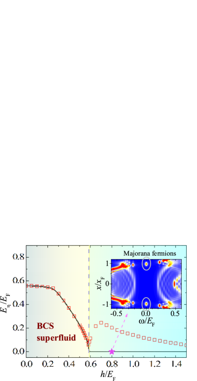
Figure 1: (color online) Zero-temperature phase diagram without solitons at $\gamma=2.2$ and $\lambda=1.5E_{F}/k_{F}$, determined from the behavior of the two lowest-energy particle solutions (with $E_{\eta}\geq 0$) in the Bogoliubov quasiparticle spectrum (shown by the solid line and empty squares, respectively). The topological phase transition occurs at about $h\simeq 0.59E_{F}$. As a result, two zero-energy Majorana fermions emerge at the trap edges, as shown in the inset, plotting the local density of states for the case $h=0.8E_{F}$. They are highlighted by two grey circles.

We note that in low dimensions phase fluctuations are generally enhanced due to the reduced dimenionality. As a result, in one dimension a true long-range order (i.e., characterized by an order parameter) is ruled out by the well-known Mermin–Wagner–Hohenberg theorem Mermin1966 ; Hohenberg1967 . Nevertheless, at zero temperature the 1D pair correlation shows a slow power-law decay, much slower than an exponential decay expected for a normal state, as predicted by using bosonization or exact Bethe ansatz approach Guan2013 . Thus, we anticipate that the assumption of an order parameter and the use of mean-field BdG equations may still provide a useful approximation. Indeed, without spin-orbit coupling, we have checked that the mean-field approach leads to reasonably accurate equation of state for a weak-coupling uniform Fermi gas, compared with the exact Gaudin-Yang solution Liu2007 . In harmonic traps, the mean-field theory also predicts very similar density profiles as the Bethe ansatz approach (within the local density approximation) Liu2007 . Therefore, in the presence of spin-orbit coupling, we assume that our mean-field treatment may qualitatively capture the essential physics of fermionic solitons.

II.2 Solitonic order parameter

A stationary dark soliton is characterized by a $\pi$-phase jump. In this case, the order parameter may be chosen to be real and a stationary soliton at the point node $x_{1}$ may take the following form for the order parameter:

$$\Delta\left(x\right)=\left|\Delta\left(x\right)\right|\exp\left[i\pi\Theta\left(x-x_{1}\right)\right],$$ (20)

where $\Theta(x)$ is the Heaviside step function. Similarly, the order parameter of a soliton train with point nodes at $x_{i}$ ($i=1,2,3,\cdots$) is given by,

$$\Delta\left(x\right)=\left|\Delta\left(x\right)\right|\exp\left[i\pi\sum_{i}\Theta\left(x-x_{i}\right)\right].$$ (21)

In numerical calculations, we calculate the order parameter through Eq. (17) and then update it by phase-imprinting the $\pi$-phase jumps with the use of Eq. (20) or Eq. (21). The solitonic order parameter is obtained self-consistently, after a number of iterations up to convergence.

II.3 Phase diagram without solitons

The solution of the BdG equations without solitons has been discussed in detail in earlier works Liu2012b ; Liu2013 ; Jiang2014 . In Fig. 1, we present the typical phase diagram at zero temperature for a spin-orbit coupled Fermi gas with $N=60$ atoms at the interaction strength $\gamma=2.2$ and spin-orbit coupling strength $\lambda=1.5E_{F}/k_{F}$. Here, we use the Thomas-Fermi energy and wavevector of a non-interacting trapped Fermi gas, $E_{F}=(N/2)\hbar\omega$ and $k_{F}=\sqrt{2mE_{F}}$, as the units of energy and wavevector, respectively. The units of length are given by the Thomas-Fermi radius, $x_{F}=\sqrt{N\hbar/(m\omega)}$. Throughout this work, we focus on the case of zero temperature and shall use the same total number of atoms ($N=60$), interaction parameter ($\gamma=2.2$) and spin-orbit coupling strength ($\lambda=1.5E_{F}/k_{F}$), unless otherwise specified. For the basis expansion, we have considered 540 single-particle eigenstates of the harmonic oscillator $\mathcal{H}_{S}$ and have taken a cut-off energy $E_{c}=15E_{F}=450\hbar\omega$, above which we use the local density approximation Liu2012b ; Liu2013 .

Fig. 1 shows the energies of the two lowest-energy particle solutions with $E_{\eta}\geq 0$, plotted respectively by using the solid line and empty squares. A topological phase transition occurs at a critical effective Zeeman field $h_{c}\simeq 0.59E_{F}$ Lutchyn2010 ; Oreg2010 ; footnote1 , as revealed by $\min\{E_{\eta}\}$ (solid line). At a small Zeeman field $h<h_{c}$, the Fermi gas is a standard BCS superfluid, with a fully gapped quasiparticle energy spectrum (i.e., $\min\{E_{\eta}\}>0$). Above the threshold, $h>h_{c}$, the quasiparticle energy spectrum is again gapped in the bulk, as seen from the empty squares. However, gapless edge excitations - Majorana fermions - emerge at the trap edges. This is particularly evident when we plot the local density of states in the inset. Two (nearly) zero-energy Majorana fermions - well localized at the trap edges as highlighted by the two grey circles - are clearly visible.

It is useful to note that Majorana fermions may acquire an exponentially small energy due to the finite size of the harmonic trap Potter2010 . The typical spatial extension of the localized Majorana wave-function $\xi_{M}$ is at the order of the coherence length $\xi_{c}=\hbar v_{F}/\Delta$, where $v_{F}$ and $\Delta$ are the unperturbed local Fermi velocity and pairing gap at the trap edge Potter2010 . For the two Majorana fermions shown in the inset of Fig. 1, we estimate that $\xi_{M}\sim 0.1x_{F}$ (see also Fig. 4). Therefore, the exponentially small overlap between two Majorana fermion wave-functions $\Phi_{L}$ and $\Phi_{R}$, i.e., $\mathcal{O}=\left\langle\Phi_{L}|\Phi_{R}\right\rangle\sim\exp(-L/\xi_{M})$, where $L\simeq 2x_{F}$ is the distance between two Majorana fermions, leads to an exponentially small energy (splitting) of Majorana fermions,

$$\frac{E}{E_{F}}\sim\mathcal{O}\sim\exp\left(-\frac{L}{\xi_{M}}\right)\sim 10^{-9}.$$ (22)

This is consistent with our numerical finding that the energy of Majorana fermions $E\sim 10^{-10}E_{F}$.

III Single soliton

Here we consider the behavior of a single dark soliton. The case of multiple dark solitons will be discussed in the next section.

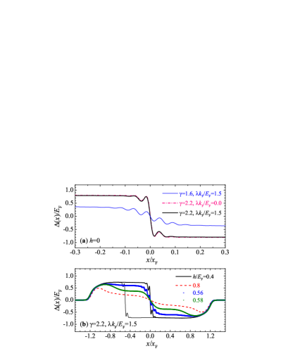
Figure 2: (color online) (a) The solitonic pairing gap $\Delta(x)$ at zero Zeeman field $h=0$ and at different interaction strengths $\gamma$ and spin-orbit coupling strengths $\lambda$, when a $\pi$-phase jump is imprinted at $x_{1}=0$. (b) The solitonic $\Delta(x)$ at nonzero Zeeman fields [$h/E_{F}=0.4$ (thick solid line), $0.56$ (crosses), $0.58$ (daggers) or $0.8$ (dashed line)] and at $\gamma=2.2$ and $\lambda=1.5E_{F}/k_{F}$. For the case of $h=0.4E_{F}$, we also consider a soliton at $x_{1}=-0.5x_{F}$ and plot the result with a thin solid line.

III.1 Order parameters

In Fig. 2, we report the pairing gap profile in the presence of a single dark soliton, at zero Zeeman field (a) or finite Zeeman fields (b). The order parameter crosses zero at the position of the soliton $x_{1}$ and hence creates a point node. At small Zeeman fields, it exhibits two length scales around the point node Antezza2007 : a fast oscillation with length scale of $k_{F}^{-1}$, and a slower healing with length scale $\xi_{c}=\hbar v_{F}/\Delta$. Here, $v_{F}$ and $\Delta$ are the unperturbed local Fermi velocity and pairing gap at the point node $x_{1}$, respectively. The former length scale is essentially independent of the interaction parameter and the spin-orbit coupling strength. Thus, as in the case of a vortex in 2D Fermi gases Hu2007b , we may safely identify the oscillation as the Friedel oscillation. For the coherence length, we find that $\xi_{c}\simeq 3k_{F}^{-1}$ at $\gamma=2.2$. It increases with decreasing interaction parameter, as expected.

For a spin-orbit coupled Fermi gas, it is interesting to see (Fig. 2(b)) that the Friedel oscillation suddenly ceases to exist when the Zeeman field is above a threshold, $h_{c}\simeq 0.57E_{F}$. Actually, this point corresponds to the topological phase transition in the presence of a single dark soliton, which we shall now discuss in greater detail.

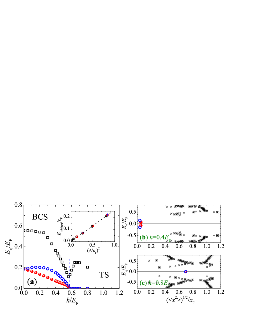
Figure 3: (color online) (a) The energies of the three lowest-energy particle solutions with $E_{\eta}\geq 0$, as a function of the Zeeman field in the case of a single dark soliton at $x_{1}=0$. The solid and empty circles show Andreev bound states localized near the soliton, while the empty squares correspond to the lowest-energy particle state in the bulk. The vertical dashed line separates the BCS and topological superfluid phases. The inset shows the minigap at $h=0$ and at different interaction parameters $\gamma$ and spin-orbit coupling strengths [$\lambda k_{F}/E_{F}=1.5$ (circles), $1.0$ (squares) and $0.0$ (daggers)], as a function of the square of the local pairing gap, $\Delta^{2}/\epsilon_{F}^{2}$. The dashed line is the linear fit $E_{\textrm{minigap}}=0.26\Delta^{2}/\epsilon_{F}$. (b) and (c) The spatial distribution of Bogoliubov quasiparticle energy spectrum at $h=0.4E_{F}$ and $h=0.8E_{F}$, respectively. The Andreev bound states near the soliton are highlighted by empty and solid circles. Here, we approximately characterize the location of a quasiparticle by using its wave-function: $\sqrt{\left\langle x^{2}\right\rangle}=\{\int dx\>x^{2}\sum_{\sigma}[u_{\sigma}^{2}\left(x\right)+\nu_{\sigma}^{2}\left(x\right)]\}^{1/2}$, if the wave-function is well-localized at a certain point. Otherwise, $\sqrt{\left\langle x^{2}\right\rangle}$ characterizes the width of the wave-function.

III.2 Andreev bound states and Majorana fermions

In the presence of a single dark soliton, the topological phase transition point can also be determined from the Bogoliubov quasiparticle spectrum. In Fig. 3(a), we plot the energies of the three lowest-energy particle solutions as a function of the Zeeman field, while in Figs. 3(b) and 3(c), we show the characteristic spectrum before and after the topological transition. The transition is associated with the closing and reopening of the energy gap in the bulk Qi2011 ; Liu2012a ; Liu2012b ; Wei2012 ; Lutchyn2010 ; Oreg2010 , see, for example, the empty squares in Fig. 3(a) for the lowest-energy bulk state in the particle branch. Thus, we determine that the transition occurs at the critical field $h_{c}\simeq 0.57E_{F}$, which is slightly smaller than the threshold $h_{c}\simeq 0.59E_{F}$ in the absence of the dark soliton (see Fig. 1).

In the topologically-trivial BCS superfluid phase, we find two Andreev-like bound states that reside near the point node of the soliton. Their existence is easy to understand from the density dip of the solitonic order parameter, which basically creates an effective confinement potential of length scale $\xi_{c}$ for quasiparticles. As a result, localized states develop, with a characteristic energy of the order of $\hbar^{2}/(m\xi_{c}^{2})=\Delta^{2}/(2\epsilon_{F})$, where $\epsilon_{F}$ is the local Fermi energy. These are reminiscent of the well-known Caroli-de Gennes-Matricon states in a vortex core in 2D Fermi gases Caroli1964 .

At zero Zeeman field, the two Andreev bound states are degenerate in energy, which is nonzero and is called the minigap in the context of superconductors in solid state physics. In the weakly-interacting limit, as shown in the inset of Fig. 3(a), we have checked that, to a very good approximation,

$$E_{\textrm{minigap}}\simeq 0.26\frac{\Delta^{2}}{\epsilon_{F}}.$$ (23)

With increasing Zeeman field, the energies of the two Andreev bound states initially split: one increases and the other decreases. However, when $h>0.2E_{F}$, both energies gradually decrease to zero as $h$ nears the topological transition. A typical energy spectrum before the transition at $h=0.4E_{F}$ is shown in Fig. 3(b), plotted as a function of the approximate location of each quasiparticle state,

$$\sqrt{\left\langle x^{2}\right\rangle}=\left[\int dx\>x^{2}\sum_{\sigma}\left(u_{\sigma}^{2}\left(x\right)+\nu_{\sigma}^{2}\left(x\right)\right)\right]^{1/2}.$$ (24)

The two Andreev bound states, represented by the empty and solid circles footnote3 , are clearly seen near the point node of the soliton at $x_{1}=0$. The highly-localized wavefunctions of the lowest-energy bound state, corresponding to the solid circle, are plotted in Fig. 4(a).

Approaching the critical Zeeman field $h_{c}\simeq 0.57E_{F}$, the energies of the two Andreev bound states tend to zero. The energies of some bulk states also vanish. The interference of these nearly zero-energy modes leads to a huge reconstruction of the quasiparticle spectrum across the topological transition. Immediately after the transition, with the reopening of the energy gap in the bulk, we observe that one of the Andreev bound states merges with bulk states and therefore can no longer be identified as a localized state. At the same time, two zero-energy edge states appear at the trap edges. As a result, we find four Majorana fermions when the system is in the topological phase: two at the edges and the other two near the soliton footnote3 . Physically, the number of Majorana fermions may be understood from the fact that a single dark soliton effectively splits the Fermi gas into two, each of which could host two Majorana fermions. In the case of multiple dark solitons, we therefore anticipate that the total number of Majorana fermions would be $2n+2$, where $n$ is the number of solitons. This expectation is confirmed by our numerical calculations.

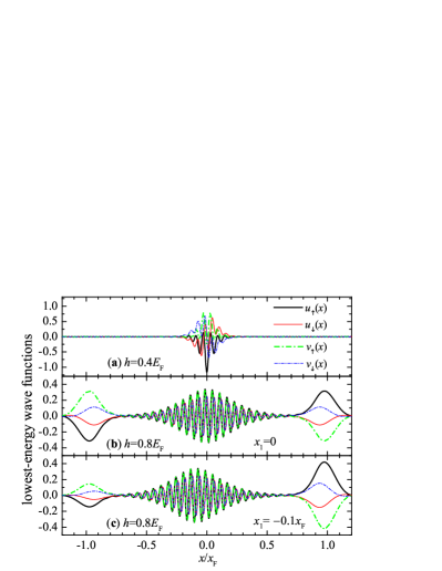
Figure 4: (color online) The wavefunctions of the lowest-energy Andreev bound states in the BCS superfluid phase at $h=0.4E_{F}$ (a) or in the topologically-nontrivial superfluid phase at $h=0.8E_{F}$ (b and c). In the latter case, the wavefunctions strongly interfere with that of Majorana fermions at the trap edges. The superposition persists when we place the dark soliton in a less symmetric position $x_{1}=-0.1x_{F}$.

In Figs. 4(b) and 4(c), we examine the wave functions of the four Majorana fermions. Since all four states are degenerate with zero energy, they may be mutually-superposed. The interference leads to very similar wavefunctions, so in the figure, only one of the four is plotted. The bond and anti-bond superpositions of the well-localized Majorana wavefunctions, presumably one at the point node of the soliton and the other two at the edges, are fairly clear (see the next paragraph for more discussions) Xu2014 . Each of these localized wavefunctions satisfies the symmetry of $u_{\sigma}\left(x\right)=\pm\nu_{\sigma}^{*}\left(x\right)$, which is precisely the required symmetry for Majorana fermions. As a result, the approximate location $\sqrt{\left\langle x^{2}\right\rangle}$ of the four Majorana fermions is exactly the same (i.e., ill-defined), as shown in Fig 3(c). This superposition is very robust with respect to the position of the dark soliton, as can be seen in Fig. 4(c). When we displace the dark soliton away from the origin to the left ($x_{1}=-0.1x_{F}$), the superposition remains, but the relative weights of the Majorana wavefunctions localized at the two edges are no longer equal.

It is important to note that, despite the superposition in wavefunctions, the energies of all the Majorana fermions are nearly zero (i.e., about $10^{-10}E_{F}$ in our numerical calculations) Xu2014 . This fact is consistent with the earlier observation that the only one Majorana fermion wave-function at the point node of the soliton is superposed with the two edge Majorana fermions, so that the energy splitting is exponentially small as in Eq. (22). Otherwise, if the two solitonic Majorana fermions near the point node do interfere with each other, we would rather anticipate a sizable energy splitting $E/E_{F}\sim e^{-L/\xi_{M}}\sim 1$, since now the distance $L\sim 0$.

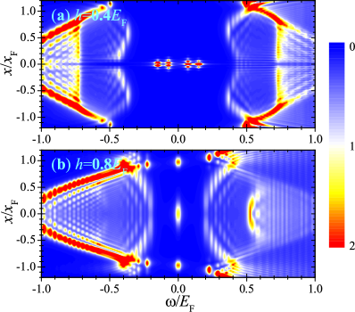
Figure 5: (color online) Local density of states of a BCS superfluid at $h=0.4E_{F}$ (a) and of a topologically-nontrivial superfluid at $h=0.8E_{F}$ (b), when a single dark soliton is created at $x_{1}=0$. In the topological phase, the two Majorana fermions near the point node of the dark soliton (at $x_{1}=0$) are not distinguishable because of the superposition of the wavefunctions. The color map indicates the magnitude of the local density of states in units of $n_{F}/E_{F}$.

III.3 Experimental detection of Majorana fermions

We now turn to consider the experimental observation of the two additional Majorana fermions localized at the point node of the dark soliton. A direct and convenient way is to use spatially-resolved radio-frequency (rf) spectroscopy, which acts as a cold-atom analog of scanning tunneling microscopy (STM) and measures the local density of states Shin2007 ; Jiang2011 . In Fig. 5, we show the local density of states $\rho(x,\omega)$ before and after the topological transition. In the BCS superfluid phase (a), the solitonic Andreev bound states can be easily identified. In the topologically-nontrivial phase (b), we can clearly see the two zero-energy Majorana fermions residing at the two trap edges. In addition, there is a zero-energy response near the origin, arising from the two Majorana fermions localized near the dark soliton. However, due to their superposition (i.e., overlapping wave functions), they are not individually resolvable.

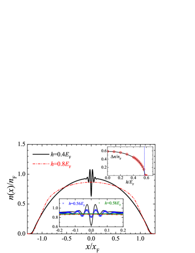
Figure 6: (color online) The total density profile in the presence of a single dark soliton at $x_{1}=0$. The solid and dashed lines show the results at $h=0.4E_{F}$ and $h=0.8E_{F}$, respectively. The inset at the bottom is an enlarged view around the origin $x=0$, with additional results near the topological transition at $h=0.56E_{F}$ (crosses) and at $h=0.58E_{F}$ (daggers). The inset at the top right top shows the oscillation amplitude $\Delta n$ of the density profile near the origin, $\Delta n=n_{\textrm{max}}-n_{\textrm{min}}$, where $n_{\textrm{max}}$ and $n_{\textrm{min}}$ are the maximum and minimum densities, respectively.

Alternatively, the existence of the soliton-induced Majorana fermions may be indirectly deduced from the total density profile, which could be measured via in-situ or time-of-flight absorption imaging. In Fig. 6, we present the density profile at two Zeeman field-strengths. Before the topological transition at $h=0.4E_{F}$ (solid line), there is an apparent oscillation with spatial period $\sim k_{F}^{-1}$, in accord with the Friedel oscillation in the solitonic order parameter (see Fig. 2). As we approach the topological transition point at the critical field strength $h_{c}\simeq 0.57E_{F}$, the amplitude of the density oscillation $\Delta n=n_{\textrm{max}}-n_{\textrm{min}}$, where $n_{\textrm{max}}$ and $n_{\textrm{min}}$ are respectively the maximum and minimum densities near the soliton, rapidly decreases and vanishes precisely at the transition (see the top right inset of Fig. 6). After the topological transition (see, for example, the dashed line at $h=0.8E_{F}$ in the main figure), the density profile becomes flat and the peak density at the trap center is essentially independent of the Zeeman field. The disappearance of the density oscillation is associated with the formation of the solitonic Majorana fermion modes, whose occupation significantly contributes to the total density because of the large amplitude of their localized wavefunctions (see Fig. 4(b)). This is very similar to what happens in the vortex core of a topological superfluid Liu2012a . There the core density is also greatly affected by the formation and occupation of the vortex-core Majorana fermion modes.

In connection with current experiments, we may consider a spin-orbit coupled ⁴⁰K Fermi gas in the presence of a tight 2D optical lattice, with an axial trapping frequency $\omega=2\pi\times 116$ Hz Wang2012 . For the typical number of total atoms $N=60$ in each tube of a 1D Fermi cloud, the Fermi temperature $T_{F}$ is about $200$ nK. We may take $k_{R}\simeq 0.75k_{F}$ and then the recoil energy is $E_{R}\simeq 0.56E_{F}$. The topological phase transition at low temperatures (i.e., $T<0.1T_{F}\simeq 20$ nK) takes place at the critical Zeeman field $h_{c}\simeq 0.6E_{F}\simeq E_{R}$, which corresponds to a critical Rabi frequency $\Omega_{R}\simeq 2E_{R}$. The size of the Fermi cloud is about $x_{F}\simeq 12$ $\mu m$. To resolve the zero-energy Majorana modes by rf spectroscopy, we may require the frequency/energy resolution to be better than $2\pi\times 100$ Hz. On the other hand, for the in-situ density profile, the spatial resolution needed to measure the amplitude of the density oscillations is about $0.5\mu m$. Thus, it seems more practical to use absorption imaging after some time-of-flight, if we assume that the structure of density oscillations survives for a short expansion time.

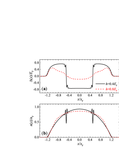
Figure 7: (color online) The solitonic order parameter (a) and the total density distribution (b) in the presence of two dark solitons (placed at $x_{1}=-0.5x_{F}$ and $x_{2}=+0.5x_{F}$), at two Zeeman fields: $h=0.4E_{F}$ (solid line) and $h=0.8E_{F}$ (dashed line).

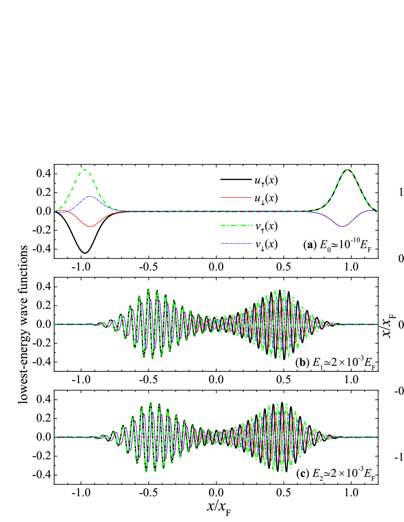
Figure 8: (color online) (a, b and c) The wave-functions of three Majorana fermions of a topological superfluid at $h=0.8E_{F}$, in the presence of two dark solitons at $x_{1}=-0.5x_{F}$ and $x_{2}=+0.5x_{F}$. The energy of each Majorana fermion is indicated. (d) The corresponding local density of state within the bulk energy gap. The color indicates the magnitude of the local density of states, see, for example, Fig. 5.

IV Multiple solitons

We now consider a soliton train. Without loss of generality, let us focus on the case of two dark solitons. Other cases with three or more dark solitons were also examined and so far we have not found additional, qualitatively different results.

In Fig. 7, we plot the solitonic order parameter and the total density distribution, when the two solitons are placed at $x_{1}=-0.5x_{F}$ and $x_{2}=+0.5x_{F}$. Qualitative features such as the Friedel oscillations in the order parameter and density profile near the point nodes of the solitons in the BCS superfluid ($h=0.4E_{F}$, solid line), can be easily understood analogously to the case of a single dark soliton, as discussed earlier (cf. Figs. 2 and 6).

In Fig. 8, we present the wavefunctions of three Majorana fermions in the topological phase (a, b and c) and their manifestation in the spatially-resolved rf spectrum (d). In total, there are six Majorana fermions, localized pair-wise at the trap edges and at the point nodes of the solitons. Only three of them are shown, one out of each pair, owing to the particle-hole symmetry. Unlike in the case of a single soliton, the two Majorana edge modes do not interfere with the solitonic Majorana fermions and hence have essentially zero energy (i.e., $E\sim 10^{-10}E_{F}$) due to the exponentially small overlap in their wavefunctions. In contrast, the overlap of the two solitonic Majorana fermion wavefunctions - originating from the two solitons - is significant. This leads to a nonzero energy for each solitonic Majorana fermion, which, following Eq. (22), is of the order of

$$\frac{E}{E_{F}}\sim\exp\left(-\frac{L}{\xi_{M}}\right)\sim 10^{-3}.$$ (25)

Here, in the estimation, we have used the distance $L\sim x_{F}$ and a bit larger localization length scale $\xi_{M}\sim 0.2x_{F}$ for the two solitonic Majorana wave-functions shown in Figs. 8(b) and 8(c).

V Conclusions

To summarize, we have investigated the behavior of dark solitons in a one-dimensional topological superfluid, in the context of ultracold atomic Fermi gases with spin-orbit coupling and an external Zeeman field Wang2012 ; Liu2012b . We have predicted that each dark soliton can host two Majorana fermions localized at its point node, which are detectable through the techniques of spatially-resolved radio-frequency spectroscopy or absorption imaging. Therefore, the well-known technique of creating dark solitons via phase imprinting also allows one to create solitonic Majorana fermions. These Majorana fermions can then find realistic applications in, e.g., topological quantum information processing and quantum computation. This scheme is very similar to the idea of using a vortex lattice in a two-dimensional topological superfluid, where the Majorana fermions at the vortex cores are used as qubits Ivanov2001 . In current cold-atom experiments, it would be much easier to engineer a soliton train than to create a vortex lattice. For the purpose of exchanging solitons at different positions to demonstrate the non-Abelian statistics of Majorana fermions, in future studies it would be interesting to understand traveling grey solitons characterized by a complex order parameter and nonzero velocity Liao2011 ; Scott2011 ; Spuntarelli2011 .

References

- (1) For a review, see D. J. Frantzeskakis, J. Phys. A 43, 213001 (2010), and references therein.
- (2) S. Burger, K. Bongs, S. Dettmer, W. Ertmer, K. Sengstock, A. Sanpera, G. V. Shlyapnikov, and M. Lewenstein, Phys. Rev. Lett. 83, 5198 (1999).
- (3) J. Denschlag, J. E. Simsarian, D. L. Feder, C. W. Clark, L. A. Collins, J. Cubizolles, L. Deng, E. W. Hagley, K. Helmerson, W. P. Reinhardt, S. L. Rolston, B. I. Schneider, and W. D. Phillips, Science 287, 97 (2000).
- (4) J. Dziarmaga and K. Sacha, Laser Phys. 15, 674 (2005).
- (5) M. Antezza, F. Dalfovo, L. P. Pitaevskii, and S. Stringari, Phys. Rev. A 76, 043610 (2007).
- (6) R. Liao and J. Brand, Phys. Rev. A 83, 041604 (2011).
- (7) R. G. Scott, F. Dalfovo, L. P. Pitaevskii, and S. Stringari, Phys. Rev. Lett. 106, 185301 (2011).
- (8) A. Spuntarelli, L. D. Carr, P. Pieri, and G. C. Strinati, New. J. Phys. 13, 035010 (2011).
- (9) A. Cetoli, J. Brand, R. G. Scott, F. Dalfovo, and L. P. Pitaevskii, Phys. Rev. A 88, 043639 (2013).
- (10) C. Caroli, P. G. de Gennes, and J. Matricon, Phys. Lett. 9, 307 (1964).
- (11) T. Yefsah, A. T. Sommer, M. J. H. Ku, L. W. Cheuk, W. Ji, W. S. Bakr, and M. W. Zwierlein, Nature (London) 499, 426 (2013).
- (12) M. J. H. Ku, W. Ji, B. Mukherjee, E. Guardado-Sanchez, L. W. Cheuk, T. Yefsah, and M. W. Zwierlein, Phys. Rev. Lett. 113, 065301 (2014).
- (13) X.-L. Qi and S.-C. Zhang, Rev. Mod. Phys. 83, 1057 (2011).
- (14) P. Wang, Z.-Q. Yu, Z. Fu, J. Miao, L. Huang, S. Chai, H. Zhai and J. Zhang, Phys. Rev. Lett. 109, 095301 (2012).
- (15) L. W. Cheuk, A. T. Sommer, Z. Hadzibabic, T. Yefsah, W. S. Bakr, and M. W. Zwierlein, Phys. Rev. Lett. 109, 095302 (2012).
- (16) R. A. Williams, M. C. Beeler, L. J. LeBlanc, K. Jimenez-Garcia, and I. B. Spielman, Phys. Rev. Lett. 111, 095301 (2013).
- (17) E. Majorana, Nuovo Cimennto 14, 171 (1937).
- (18) F. Wilczek, Nat. Phys. 5, 614 (2009).
- (19) X.-J. Liu, L. Jiang, H. Pu, and H. Hu, Phys. Rev. A 85, 021603(R) (2012).
- (20) C. Nayak, S. Simon, A. Stern, M. Freedman, and S. Das Sarma, Rev. Mod. Phys. 80, 1083 (2008).
- (21) D. A. Ivanov, Phys. Rev. Lett. 86, 268 (2001).
- (22) Y. Xu, L. Mao, B. Wu, and C. Zhang, Phys. Rev. Lett. 113, 130404 (2014).
- (23) X.-J. Liu and H. Hu, Phys. Rev. A 85, 033622 (2012).
- (24) R. Wei and E. J. Mueller, Phys. Rev. A. 86, 063604 (2012).
- (25) X.-J. Liu, Phys. Rev. A 87, 013622 (2013). Note that, the spin-orbit coupling strength in this work should be , instead of as mentioned in the text.
- (26) L. Jiang, E. Tiesinga, X.-J. Liu, H. Hu, and H. Pu, Phys. Rev. A 90, 053606 (2014).
- (27) T. Bergeman, M. G. Moore, and M. Olshanii, Phys. Rev. Lett. 91, 163201 (2003).
- (28) H. Hu, X.-J. Liu, and P. D. Drummond, Phys. Rev. Lett. 98, 070403 (2007).
- (29) X.-J. Liu, H. Hu, and P. D. Drummond, Phys. Rev. A 76, 043605 (2007).
- (30) X.-J. Liu, H. Hu, and P. D. Drummond, Phys. Rev. A 78, 023601 (2008).
- (31) Y.-A. Liao, A. S. C. Rittner, T. Paprotta, W. Li, G. B. Partridge, R. G. Hulet, S. K. Baur, and E. J. Mueller, Nature (London) 467, 567 (2010).
- (32) N. D. Mermin and H. Wagner, Phys. Rev. Lett. 17, 1133 (1966).
- (33) P. C. Hohenberg, Phys. Rev. 158, 383 (1967).
- (34) For a review, see, for example, X.-W. Guan, M. T. Batchelor, and C. Lee, Rev. Mod. Phys. 85, 1633 (2013).
- (35) R. M. Lutchyn, J. D. Sau, and S. D. Sarma, Phys. Rev. Lett. 105, 077001 (2010).
- (36) Y. Oreg. G. Refael, and F. von Oppen, Phys. Rev. Lett. 105, 177002 (2010).
- (37) In a homogeneous spin-orbit coupled Fermi gas, the critical field is given by , at which the energy gap of the system closes Lutchyn2010 ; Oreg2010 . In harmonic traps with our chosen parameters, the topological transition occurs first at the trap center. Thus, the critical field is where is the pairing gap at the trap center.
- (38) A. C. Potter and P. A. Lee, Phys. Rev. Lett. 105, 227003 (2010).
- (39) H. Hu, X.-J. Liu, and P. D. Drummond, Phys. Rev. Lett. 98, 060406 (2007).
- (40) If we take into account their hole partners, these two physical Andreev bound states may be regarded as four modes. This interpretation is useful for understanding the four zero-energy Majorana fermions in the presence of a single soliton, a pair emerging from each Andreev bound state.
- (41) Y. Shin, C. H. Schunck, A. Schirotzek, and W. Ketterle, Phys. Rev. Lett. 99, 090403 (2007).
- (42) L. Jiang, L. O. Baksmaty, H. Hu, Y. Chen, and H. Pu, Phys. Rev. A 83, 061604(R) (2011).