Hierarchical multiscale modeling for flows in fractured media using Generalized Multiscale Finite Element Method
Abstract
In this paper, we develop a multiscale finite element method for solving flows in fractured media. Our approach is based on Generalized Multiscale Finite Element Method (GMsFEM), where we represent the fracture effects on a coarse grid via multiscale basis functions. These multiscale basis functions are constructed in the offline stage via local spectral problems following GMsFEM. To represent the fractures on the fine grid, we consider two approaches (1) Discrete Fracture Model (DFM) (2) Embedded Fracture Model (EFM) and their combination. In DFM, the fractures are resolved via the fine grid, while in EFM the fracture and the fine grid block interaction is represented as a source term. In the proposed multiscale method, additional multiscale basis functions are used to represent the long fractures, while short-size fractures are collectively represented by a single basis functions. The procedure is automatically done via local spectral problems. In this regard, our approach shares common concepts with several approaches proposed in the literature as we discuss. Numerical results are presented where we demonstrate how one can adaptively add basis functions in the regions of interest based on error indicators. We also discuss the use of randomized snapshots ([2]) which reduces the offline computational cost.
1 Introduction
Many porous media flow and transport processes are dominated by the presence of fractures. The fractures present high conductivity conduits and their effects need to be captured accurately in the simulations. Because the fractures have very small width, they are often represented as zero thickness objects in numerical simulations. Because there are many fractures of different lengths (connected or not connected), the problem is inherently multiscale and efficient multiscale techniques are needed to represent their effects.
In this paper, we present an application of Generalized Multiscale Finite Element Method for flows in fractured media. The study of flow in fractured media on the fine grid has been conducted in numerous papers. These models applied various fracture models, such as the Discrete Fracture Model (DFM), Embedded Fracture Model (EFM), the single-permeability model, and the multiple-permeability models ([22, 1, 20, 17, 12, 23]). Though these approaches are designed for fine-scale simulations, a number of these approaches represent the fractures at a macroscopic level. For example, multiple-permeability models represent the network of connected fractures macroscopically by introducing several permeabilities in each block. The EFM ([19, 18, 17]) models the interaction of fractures with the fine-grid blocks separately for each block. These approaches can be generalized by incorporating the interaction of fractures and permeability heterogeneities locally which can lead to efficient upscaling techniques. Some general upscaling techniques for flows in fractured network are presented in [5, 11], where the authors introduce the fracture and matrix interaction parameters hierarchically.
In recent papers [13], several multiscale approaches are proposed for representing the fracture effects. These approaches share common concepts with the methods that we discuss here in a sense that they add new degrees of freedom to represent the fractures on a coarse grid. The main difference is that our approaches use local spectral problems accompanied by adaptivity to detect the region where to add new basis functions. In this regard, the procedure of finding multiscale basis functions and the enrichment procedure is different from existing techniques.
In this paper, we use a general multiscale finite element framework, GMsFEM. GMsFEM is a flexible general framework that generalizes the Multiscale Finite Element Method (MsFEM) ([15]) by systematically enriching the coarse spaces and taking into account small scale information and complex input spaces. In this work, we use Discrete Fracture Model (DFM) ([21, 14, 24, 16]) for the simulation of the fine-scale problem as well as in the construction of spectral problem for the GMsFEM. In GMsFEM approach, as in many multiscale model reduction techniques, which divides the computation into two stages: the offline stage and the online stage. In the offline stage, a small dimensional space is constructed that can be used in the online stage to construct multiscale basis functions. These multiscale basis functions can be re-used for any input parameter to solve the problem on a coarse grid. The main idea behind the construction of offline and online spaces is the selection of local spectral problems and the selection of the snapshot space. In [7], we propose several general strategies. The main idea of this paper is to combine GMsFEM with DFM and/or EFM to solve the flow problem in fractured media. We present a multiscale basis construction, adaptivity, and the use of randomized snapshots to reduce the computational cost.
Our approaches share some common concepts with hierarchical fracture modeling proposed by Lee et al. [17], where the main idea is to homogenize small-length fractures (with the length smaller than the coarse block), while represent the large-length fractures. Our methods via local multiscale basis functions homogenizes small-size fractures (by lumping their effect into a single-per-node multiscale basis function) and represent the long-size fractures in each coarse block. A global coupling, such as finite element in this case, recover an accurate representation of long size fractures by coupling all the information together.
We present several numerical examples to illustrate the performance of the proposed approach. We consider the fine-scale fracture representations using DFM, EFM as well as coupled DFM and EFM, where the shorter fractures are represented by DFM and the longer ones EFM. All the numerical results indicate that the proposed GMsFEM is robust and accurate. Besides, we test the performance of adaptive algorithm in [4] for the problem in this paper. To reduce the computational cost, we propose the use of randomized snapshots where only a few snapshots are constructed and used to construct multiscale basis functions. We would like to emphasize that our goal is to develop and show the performance of GMsFEM for flows in fractured media and we do not make any comparisons between different fine-scale fracture models.
The rest of the paper is organized as follows. In Section 2, we present preliminaries. The fine-scale fracture modeling techniques are briefly reviewed in Section 3.1. The construction of the coarse spaces for the GMsFEM is displayed in Section 4. In Section 5, numerical results for several representative examples are showed. Finally, we conclude our paper with some remarks in Section 6.
2 Preliminaries
In this paper, we study high-contrast flow problem
| (1) |
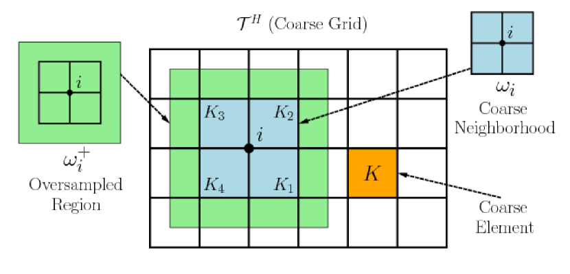
where has fractures with high values and low values in the matrix (see Figure 2 for illustration). To discretize (1), we introduce the notions of fine and coarse grids. Let be a usual conforming partition of the computational domain into finite elements (triangles, quadrilaterals, tetrahedra, etc.). We denote this partition as the coarse grid and assume that each coarse element is partitioned into a connected union of fine-grid blocks. The fine grid partition will be denoted by , and is by definition a refinement of the coarse grid . We use (where denotes the number of coarse nodes) to denote the vertices of the coarse mesh , and define the neighborhood of the node by
| (2) |
See Figure 1 for an illustration of neighborhoods and elements subordinated to the coarse discretization. We emphasize the use of to denote a coarse neighborhood, and to denote a coarse element throughout the paper.
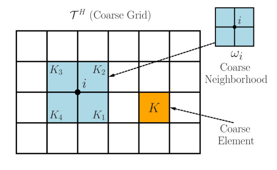

Next, we briefly outline the GMsFEM. We will consider the continuous Galerkin (CG) formulation and signify as the support of basis functions. We denote the basis functions by , which is supported in , and the index represents the numbering of these basis functions. In turn, the CG solution will be sought as . Once the basis functions are identified (see the next section), the CG global coupling is given through the variational form
| (3) |
where is used to denote the space spanned by those basis functions and , are bilinear (or linear) form corresponding to (1) defined by , and . We also note that one can use discontinuous Galerkin formulation (see e.g., [6, 3, 9]) to couple multiscale basis functions defined on .
Let be the conforming finite element space with respect to the fine-scale partition . We assume is the fine-scale solution satisfying
| (4) |
In the next section, we will introduce fine-grid discretizations for fractures. As we have mentioned above that the aperture of the fracture is very thin, and the fracture permeability is high.
3 Discretizing fractures on the fine grid
3.1 Discrete Fracture Model (DFM)
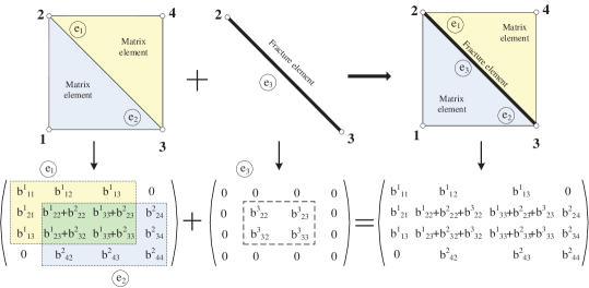
Our first approach is based on representing the fractures on the fine grid as the edges of finite element mesh. This allows meshing the fractures more accurately; however, it can be expensive when the fracture distribution is irregular. Following a standard convention, we call “matrix” the region that excludes all the fractures. In the DFM (see e.g., [1]) as implemented in this paper, we assume that the permeability does not vary along the fractures, which coincide with the edges (or faces) of finite element mesh. The fracture aperture is taken into account in the finite element discretization as a lower dimensional lines or surfaces. More precisely, the discretization of the fractures on low dimensional surfaces are added to finite element discretization of the matrix system. Below, we demonstrate this main idea in our two dimensional example.
Based on the assumptions above on the DFM, the fractures can be treated as one dimensional. One-dimensional element is introduced in addition to the two-dimensional element for the discretization of the matrix. Thus the Eqn. (1) will be discretized in two-dimensional form for the matrix and in one-dimensional form for the fractures. The whole domain can be represented by
| (5) |
where the subscript and frac represent the matrix and the fracture regions, respectively and refers to th fracture. Note that is a two-dimensional domain and is a one-dimensional domain. We write the finite element discretization corresponding to Eqn. (4) as (see also Figure 3 for illustration)
| (6) |
3.2 Embedded Fracture Model (EFM)
In this section, we present a fine-discretization of fracture network following EFM proposed by Lee et al. ([17]). EFM allows avoiding complex meshing for fracture network. We would like again to emphasize that our goal is not to compare DFM with EFM, but rather to develop GMsFEM framework which uses both fine-grid discretization techniques. In EFM, long fractures are treated as low dimensional objects and their interaction with the matrix is modeled separately. In our two dimensional simulations, we treat the long fractures separately as one-dimensional problems. Eqn. (1) can be written as
| (7) | |||
| (8) |
where and represent the interaction between the long fractures and the rest of the system. Those two terms can be calculated following [17]. We denote the linear system corresponding to the discrete form of the problem above is
| (9) |
Here, denotes the total number of long fractures, is the matrix obtained over the domain excluding the long fractures. denotes the interaction of the th long fracture with the matrix and denotes the matrix interaction with the th long fracture, where . Here, we use EFM to handle long fractures, though it can be used for shorter fractures.
4 GMsFEM
In this section, we will give a brief description of the GMsFEM for heterogeneous flow problems. More details can be found in [7, 8]. In the following, we give a general outline of the GMsFEM. Then, we will discuss the multiscale basis construction.
Offline computations:
-
Step 1
Coarse grid generation.
-
Step 2
Construction of snapshot space that will be used to compute an offline space.
-
Step 3
Construction of a small dimensional offline space by performing dimension reduction in the space of local snapshots.
If the problem has a parameter, one can use the offline space to construct multiscale basis functions in the online stage. In the above outline, the offline space can be reused if we change the input of the model. Given the computational domain, a coarse grid can be constructed and local problems are solved on coarse neighborhoods to obtain the snapshot spaces. Then, smaller dimensional offline spaces are obtained from the snapshot spaces by dimension reduction via some spectral problems.
4.1 Local basis functions
We now present the construction of the basis functions and the corresponding spectral problems for obtaining a model reduction.
In the offline computation, we first construct a snapshot space for each coarse neighborhood . The snapshot space can be the space of all fine-scale basis functions or the solutions of some local problems with various choices of boundary conditions. In [2], we use -harmonic extensions to form a snapshot space. For flows in fractured media, the snapshot vectors are computed in the same way except that we use an appropriate fine-grid discretization taking into account the fracture distribution. In specific, given a fine-scale piecewise linear function defined on , we define by
| (10) |
where on . The local problem is solved taking into consideration the fracture distribution. Later, we use randomized boundary conditions to avoid computing the full snapshot vectors and use only a few snapshot vectors. In particular, we use DFM for computing all snapshot vectors. For EFM, we follow a hierarchical approach and discretize few fractures using the interaction terms. We can also add them into the calculations of snapshot vectors; however, in the paper, we consider EFM for handling a few long fractures.
For brevity of notation we now omit the superscript , yet it is assumed throughout this section that the offline space computations are localized to respective coarse subdomains. Let be the number of functions in the snapshot space in the region , and
for each coarse subdomain . Denote
In order to construct the offline space , we perform a dimension reduction in the local snapshot space using an auxiliary spectral decomposition. The analysis in [10] motivates the following eigenvalue problem in the space of snapshots:
| (11) |
where
and
The above integrals take into account the fracture distributions (see Eqn. (6)). We present the details of later.
Here and denote analogous fine-scale matrices as defined by
where is the fine-scale basis function, and is defined in the next subsection.
To generate the offline space we then choose the smallest eigenvalues from Eqn. (11) and form the corresponding eigenvectors in the space of snapshots by setting (for ), where are the coordinates of the vector .
4.2 Global coupling
In this subsection, we discuss the offline space and the variational formulation for a continuous Galerkin approximation of Eqn. (1). We begin with an initial coarse space . Denote to be the number of coarse neighborhoods. Here, are the standard multiscale partition of unity functions defined by
| (12) | |||
for all , where is a continuous function on and is linear on each edge of . We note that pointwise energy required for the eigenvalue problems is defined as
where denotes the coarse mesh size.
We then multiply the partition of unity functions by the eigenfunctions in the offline space to construct the resulting basis functions
| (13) |
where denotes the number of offline eigenvectors that are chosen for each coarse node . We note that the construction in Eqn. (13) yields continuous basis functions due to the multiplication of offline eigenvectors with the initial (continuous) partition of unity function. Next, we define the continuous Galerkin spectral multiscale space as
| (14) |
Using a single index notation, we may write , where denotes the total number of basis functions in the space . We also construct an operator matrix (where are used to denote the nodal values of each basis function defined on the fine grid), for later use in this subsection.
Below, we will display in detail the multiscale formulation using DFM and EFM, respectively.
4.2.1 Multiscale DFM approach
We seek such that
| (15) |
Note that the offline space is an approximation of all the nodal basis, including the ones on the long fractures. Therefore, the variational form in (15) yields the following linear algebraic system
| (16) |
where denotes the nodal values of the discrete solution, and
Using the operator matrix , we may write and , where and are the standard, fine-scale stiffness matrix and forcing vector corresponding to the form in Eqn. (6). We also note that the operator matrix may be analogously used in order to project coarse scale solutions onto the fine grid.
4.2.2 Multiscale EFM approach
Similar to the multiscale DFM approach proposed above, we seek such that
However, the nodal basis on the long fractures are excluded from the offline space , i.e., the fine-scale nodal basis are used on the long fractures. It follows from Eqn. (9),
| (17) |
Note that the operator matrix may be analogously used in order to project coarse scale solutions onto the fine grid.
5 Numerical result
In this section, we will present several numerical experiments to show the performance of multiscale DFM and multiscale EFM approaches in the fracture modeling. The simulation results using multiscale DFM is shown in Subsection 5.1. In Subsection 5.2, a few tests are conducted to verify the performance of multiscale EFM approach. Moreover, we combine those two approaches in the modeling of short and long fractures and list the results in Subsection 5.3. Further, the relation between the basis selection and the types of fractures is studied in Subsection 5.4. We also present a randomized snapshot calculations to reduce the computational cost associated with computing the snapshot space.
We take the domain to be a square, set the forcing term and impose a bilinear boundary condition for the problem (1). In our numerical simulations, we use a coarse grid, and each coarse grid block is further divided into fine grid blocks. Thus, the whole computational domain is partitioned into a fine grid. The fine-scale solution is obtained by discretizing (1) following DFM with piecewise bilinear elements on the fine grid and linear one-dimensional elements over the fractures.
We recall that denotes the offline space; , and denote the fine-scale, snapshot and offline solutions, respectively. In the tables below, we will compute the error using the relative error and the energy relative error, which are defined as
| (18) |
where the weighted -norm is defined as . We will also compute the error using the same norms
| (19) |
5.1 Numerical results with DFM
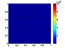
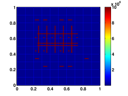
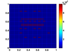
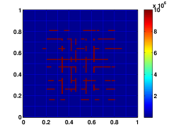
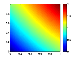
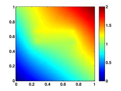
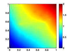
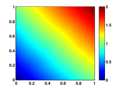
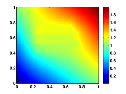
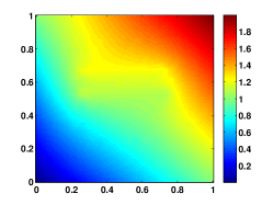
In Fig. 4, we depict three fracture fields used in the simulations below. In Fig. 4(a), there is at most one fracture in each coarse block without crossing the coarse edges, while in Figs. 4(b) and 4(c), the fractures are more complicated and intersect the edges of coarse blocks. The simulation result with fractures in Fig. 4(a) with 1 basis per coarse node is very good (with the energy error of ) because their effects can be localized. The simulation results with the other two fracture systems are shown in Tables 1 and 2, respectively. We notice that one basis function per node does not give a satisfactory for more complex fracture systems. We also show the fine-scale solutions and the snapshot solutions (i.e. the coarse-scale solution corresponding to the largest offline space we select) corresponding to fractures in Fig. 4, which are shown in Figs. 6 and 8, respectively.
The convergence history of fracture fields in Figs. 4(b) and 4(c) are displayed in Tables 1 and 2. We observe that the offline solution will converge to the fine-scale solution as we enrich the offline space in each coarse neighborhood. The energy error decreases from to as we add 4 more local basis in each coarse neighborhood from Table 1. In Tables 3 and 4, we show the numerical results for fracture fields in Figs. 5(a) and 5(b).




| (%) | (%) | |||
|---|---|---|---|---|
| (%) | (%) | |||
|---|---|---|---|---|
| (%) | (%) | |||
|---|---|---|---|---|
| (%) | (%) | |||
|---|---|---|---|---|
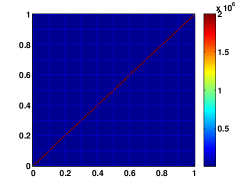
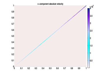
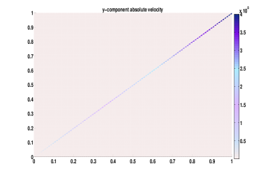
We have also performed a few simulations with uniform triangular meshes with the fracture field depicted in Fig. 5(c). We depict the fine-scale velocity components in Fig. 9. The coarse-scale velocity component of this fracture field is similar to those fracture fields above, and thus are not presented. Triangular meshes can also be used in the simulation.
5.2 Numerical results with EFM
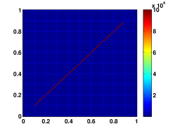
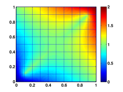
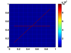
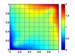
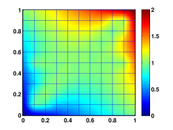
In this subsection, the numerical results using EFM are presented. As mentioned above, the main advantage of this model is that the fracture does not need to align with fine grid boundaries. The numerical results are shown in Figs. 10 and 11. Note that for this model, we have unique nodes (independent of the matrix nodes) for the fractures. The number of long fractures are quite few (e.g. there is only one fracture in Fig. 10). Therefore, it is not necessary for the upscaling over the long fractures. The classical multiscale finite element method is applied in Fig. 10 to obtain the coarse-scale solution. The corresponding weighted error and errors are and . Therefore, no spectral problem is needed for this fracture field. Similarly, for the simulation depicted in Fig. 11, the GMsFEM algorithm gives an error of and for energy error and , error respectively.

5.3 Numerical results for mutiscale DFM and EFM approach
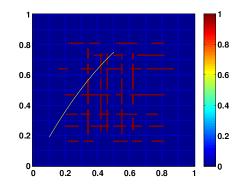
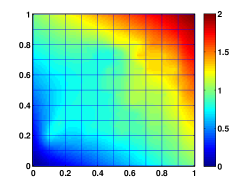
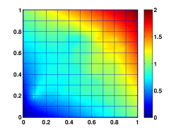
In this subsection, we will display several numerical results using DFM and EFM jointly. A heterogeneous medium with different lengths of fractures is illustrated in Fig 12(a). The coarse-scale solution and the fine-scale solution are shown in Figs 12(b) and 12(c), respectively. The fine-scale solution is calculated by the DFM over the fine mesh. We observe that the coarse-scale solution is a good approximation of the fine-scale solution. Besides, the relative energy error and relative errors are shown in Table 5. We see that the energy relative error and relative error are and when the dimension of the coarse system is 364.
| (%) | (%) | |||
|---|---|---|---|---|
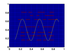
We test another heterogeneous fractured medium in Fig. 13(a). Compared with the previous heterogeneous medium, this one has a longer fracture with a curved shape. The coarse-scale solution and fine-scale solution are shown in Figs. 13(b) and 13(c). We present the errors in Table 6.

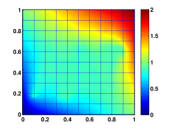
| (%) | (%) | |||
|---|---|---|---|---|
5.4 Adaptive method
In this subsection, we will discuss adaptive strategies for generating multiscale basis functions efficiently. First, we will not use extra basis functions in the regions with long fractures. This intuitive approach is based on previous findings [10]. Next, we will use the error indicators that we proposed in [4], which identify the regions adaptive enrichment is needed.
We consider the fracture fields shown in Figs. 4(b) and 4(c). As shown in these figures, both fields have channels and isolated inclusions in certain coarse neighborhoods. The local coarse spaces contain enough information about isolated inclusions because of the usage of multiscale partition of unity functions in the construction of global generalized multiscale basis. Therefore, the adaptive enrichment process takes place in the regions with long channels.
We begin with basis in each coarse node and examine the fracture field shown in Fig.4(b) following the reasoning above. We conclude that the coarse nodes with adaptive enrichment are , and . Adding 3 more basis to those coarse nodes, we can get the energy error of with the coarse space dimension of . Compare with results listed in Table 1 (coarse space of dimension and the energy error of ), we observe that with this adaptive enrichment, we can get a better offline solution with a smaller solution space.
We also test the field in Fig. 4(c). The coarse nodes with long fractures are , and . Adding 2 more basis to those coarse nodes, we can get the energy error of with the coarse space dimension of . Compare with results listed in Table 2, the energy error is with a coarse space of dimension . We can see that with this adaptive algorithm, we can get a better offline solution with a smaller solution space.
Next, we use the -based error indicator proposed in [4]. We start with basis per coarse node and take in the adaptive algorithm proposed in [4]. Comparing Table 3 with Table 7, we notice that there is a slight gain regarding to the energy error for this adaptive algorithm. In Table 3, the energy error is for an offline space of dimension , while for in the adaptive algorithm.
Next, we study the adaptive algorithm for the field in Fig. 4(c). From results in Table 2 and Table 8, we conclude that the adaptive algorithm can improve the performance of GMsFEM. Using an offline space with less basis, the adaptive enrichment algorithm can still have a better performance.
| (%) | (%) | |||
|---|---|---|---|---|
| (%) | (%) | |||
|---|---|---|---|---|
5.5 Randomized snapshots
In this section, we will investigate the oversampling randomized algorithm proposed in [2]. The main advantage of this algorithm is that it uses much fewer snapshot basis functions to calculate the offline space. Besides, the oversampling strategy is used to reduce the subgrid errors due to boundary conditions imposed to obtain the snapshot basis. We refer to Fig. 1 for an illustration of oversampling domain.
In our simulation, we set the oversampling size (two fine-grid layer around the coarse region) and buffer number for each coarse neighborhood . I.e., we generate snapshot functions in each coarse neighborhood when computing basis functions. For the sake of completeness, we list the algorithm here in Table LABEL:algorithm:random_snapshots.
| Input: | Fine grid size , coarse grid size , oversampling size , buffer number for each , |
|---|---|
| the number of local basis functions for each ; | |
| output: | Coarse-scale solution . |
| 1. | Generate oversampling region for each coarse block: , , and ; |
| 2. | Generate random vectors and obtain randomized snapshots in ; |
| Add a snapshot that represents the constant function on ; | |
| 3. | Obtain offline basis by a spectral decomposition restricted to the original domain ; |
| 4. | Construct multiscale basis functions and solve it. |
The numerical results using the permeability field shown in Fig. 13(a) are presented in Table 10. In this table, the first column shows the dimension of the offline space, and the second columns displays the ratio between the number of the randomized snapshot basis and the full snapshot basis. Then, in the following two columns, the weighted and energy error using the full snapshots are shown. At last, the results using the randomized snapshots alone is listed in the last two column. Comparing these results with those using the full snapshot space, we deduce that the multiscale randomized algorithm performs well. The relative energy error is using the randomized snapshots, which account to of the full snapshots. However, we can only get relative energy error if the full snapshots are used instead.
| Snapshot ratio (%) | All snapshots (%) | Randomized snapshots (%) | |||
|---|---|---|---|---|---|
6 Discussions and Conclusions
In this paper, we develop a multiscale finite element method for flows in fractured media. Our approach is based on Generalized Multiscale Finite Element Method (GMsFEM). Multiscale basis functions are constructed in the offline stage via local spectral problems. To represent the fractures on the fine grid, we consider two approaches (1) Discrete Fracture Model (DFM) (2) Embedded Fracture Model (EFM) and their combination. The proposed procedure automatically selects multiscale basis functions via local spectral problems.
Numerical results are presented where we demonstrate how one can adaptively add basis functions in the regions of interest based on error indicators. We consider various cases with long and short fractures. Our numerical results show that GMsFEM with much fewer degrees of freedom compared to the fine-scale simulations can capture the solution behavior accurately. Furturemore. we discuss the use of randomized snapshots ([2]) which substantially reduces the offline computational cost.
References
- [1] R. Baca, R. Arnett, and D. Langford. Modeling fluid flow in fractured porous rock masses by finite element techniques. Int. J. Num., 4:337–348, 1984.
- [2] V. Calo, Y. Efendiev, J. Galvis, and G. Li. Randomized oversampling for generalized multiscale finite element methods. http://arxiv.org/pdf/1409.7114.pdf.
- [3] E. Chung, Y. Efendiev, and W. T. Leung. Generalized multiscale finite element method for wave propagation in heterogeneous media. arXiv:1307.0123.
- [4] E. Chung, Y. Efendiev, and G. Li. An adaptive GMsFEM for high-contrast flow problems. Journal of Computational Physics, 273:54 – 76, 2014.
- [5] L. J. Durlofsky. Numerical calculation of equivalent grid bock permeability tensors for heterogeneous porous media. Water resources research, 27(5):699–708, 1991.
- [6] Y. Efendiev, J. Galvis, Li. G., and M. Presho. Generalized multiscale finite element methods. nonlinear elliptic equations. Commun. Comput. Phys., 15:733–755, 2014.
- [7] Y. Efendiev, J. Galvis, and T. Hou. Generalized multiscale finite element methods. Journal of Computational Physics, 251:116–135, 2013.
- [8] Y. Efendiev, J. Galvis, G. Li, and M. Presho. Generalized multiscale finite element methods. oversampling strategies. International Journal for Multiscale Computational Engineering, 12(6):465–484, 2014.
- [9] Y. Efendiev, J. Galvis, M. Moon, R. Lazarov, and M. Sarkis. Generalized multiscale finite element method. symmetric interior penalty coupling. Journal of Computational Physics, 255:1–15, 2013.
- [10] Y. Efendiev, J. Galvis, and X.H. Wu. Multiscale finite element methods for high-contrast problems using local spectral basis functions. Journal of Computational Physics, 230:937–955, 2011.
- [11] B. Gong, M. Karimi-Fard, and L. J. Durlofsky. Upscaling discrete fracture characterizations to dual-porosity, dual-permeability models for efficient simulation of flow with strong gravitational effects. SPE J., 13(1):58–67, 2008.
- [12] H. Hajibeygi, D. Karvounis, and P. Jenny. A loosely coupled hierarchical fracture model for the iterative multiscale finite volume method. Society of Petroleum Engineers. doi:10.2118/141991-MS.
- [13] H. Hajibeygi, D. Karvounis, and P. Jenny. A loosely coupled hierarchical fracture model for the iterative multiscale finite volume method. Society of Petroleum Engineers. doi:10.2118/141991-MS.
- [14] H. Hoteit and A. Firoozabadi. An efficient numerical model for incompressible two-phase flow in fractured media. Adv. Water Resour., 31:891–905, 2008.
- [15] T. Hou and X.H. Wu. A multiscale finite element method for elliptic problems in composite materials and porous media. J. Comput. Phys., 134:169–189, 1997.
- [16] Z. Huang, J. Yao, Y. Wang, and K. Tao. Numerical study on two-phase flow through fractured porous media. Science China-Technological Sciences, 54:2412–2420, 2011.
- [17] S.H. Lee, M.F. Lough, and C.L. Jensen. Hierarchical modeling of flow in naturally fractured formations with multiple length scales. Water resources research, 37(3):443–455, 2001.
- [18] L. Li and S. H. Lee. Efficient field-scale simulation of black oil in naturally fractured reservoir through discrete fracture networks and homogenized media. SPE Reservoir Evaluation & Engineering.
- [19] M. F. Lough, S. H. Lee, and J. Kamath. A new method to calculate effective permeability of gridblocks used in the simulation of naturally fractured reservoirs. SPE doi:10.2118/36730-PA.
- [20] M. M. Karimi-Fard and A. Firoozabadi. Numerical simulation of water injection in 2d fractured media using discrete-fracture model. SPE REE J., 4:117–126, 2003.
- [21] J. Noorishad and M. Mehran. An upstream finite element method for solution of transient transport equation in fractured porous media. Water Resour. Res., 18(3):588–596, 1982.
- [22] Yu-Shu Wu, Yuan Di, Zhijiang Kang, and Perapon Fakcharoenphol. A multiple-continuum model for simulating single-phase and multiphase flow in naturally fractured vuggy reservoirs. Journal of Petroleum Science and Engineering, 78(1):13–22, 2011.
- [23] Yu-Shu Wu, G. Qin, R. E. Ewing, Y. Efendiev, Z. Kang, and Y. Ren. A multiple-continuum approach for modeling multiphase flow in naturally fractured vuggy petroleum reservoirs. SPE-104173, presented at the 2006 SPE International Oil & Gas Conference and Exhibition in China held in Beijing, China.
- [24] N. Zhang, J. Yao, Z. Huang, and Y. Wang. Accurate multiscale finite element method for numerical simulation of two-phase flow in fractured media using discrete-fracture model. Journal of Computational Physics, 242:420–438, 2012.