Co-spatial Long-slit UV/Optical Spectra of Ten Galactic Planetary Nebulae with HST/STIS I. Description of the Observations, Global Emission-line Measurements, and CNO Abundances

Abstract

We present observations and initial analysis from an HST Cycle 19 program using STIS to obtain the first co-spatial, UV-optical spectra of ten Galactic planetary nebulae (PNe). Our primary objective was to measure the critical emission lines of carbon and nitrogen with unprecedented S/N and spatial resolution over the wavelength range 1150–10270 Å, with the ultimate goal of quantifying the production of these elements in low- and intermediate-mass stars. Our sample was selected from PNe with a near-solar metallicity, but spanning a broad range in N/O based on published ground-based and IUE spectra. This study, the first of a series, concentrates on the observations and emission-line measurements obtained by integrating along the entire spatial extent of the slit. We derived ionic and total elemental abundances for the seven PNe with the strongest UV line detections (IC 2165, IC 3568, NGC 2440, NGC 3242, NGC 5315, NGC 5882, and NGC 7662). We compare these new results with other recent studies of the nebulae, and discuss the relative merits of deriving the total elemental abundances of C, N, and O using ionization correction factors (ICFs) versus summed abundances. For the seven PNe with the best UV line detections, we conclude that summed abundances from direct diagnostics of ions with measurable UV lines gives the most accurate values for the total elemental abundances of C and N (although ICF abundances often produced good results for C). In some cases where significant discrepancies exist between our abundances and those from other studies, we show that the differences can often be attributed to their use of fluxes that are not co-spatial. Finally, we examined C/O and N/O versus O/H and He/H in well-observed Galactic, LMC, and SMC PNe, and found that highly accurate abundances are essential for properly inferring elemental yields from their progenitor stars. Future papers will discuss photoionization modeling of our observations, both of the integrated spectra and spatial variations of the UV vs. optical lines along the STIS slit lengths, which are unique to our observations.

1 Introduction

The elements carbon (C) and nitrogen (N) are present in all known life forms, and identifying the major stellar production sources of these elements is one of the most pressing problems in galactic abundance and astrobiology studies today. That C and N are synthesized and ejected by both massive stars, and by low and intermediate mass stars (0.8M$\rm{}_{\odot}\leq M\leq 8M_{\odot}$; LIMS), is not in doubt. The existence in the Galaxy of WC and WN stars with progenitor masses exceeding 20 M_⊙, as well as carbon stars and planetary nebulae (PNe) with LIMS as progenitors, suggests that the Galactic level of these elements is likely mediated by both components of the mass spectrum. The real challenge is to determine the proportional contribution that each component makes.

Numerous theorists have used stellar evolution models to predict the fraction of synthesized C and N, as a function of progenitor mass and metallicity, that LIMS eject into their PNe. Historically, optical spectra of collisionally excited emission lines in PNe have been used to determine N and O abundances from the strong emission lines of [O II] $\rm\lambda$3727 and [O III] $\rm\lambda\lambda$4959,5007 and [N II] $\rm\lambda\lambda$6548,6583. However in a majority of PNe N⁺ represents only a very minor fraction of the total N abundance, and the ratio of O⁺/O⁺⁺ has been used as an ionization correction factor (ICF) to estimate a value of N/O. In the higher ionization objects a correction is needed for unobserved O⁺³, as indicated by the amount of He⁺⁺ compared to He⁺, and the [N II] lines are exceedingly weak, making the N abundance uncertain. For C, there are no collisionally excited lines in the optical spectral region at all. Only recently have investigators attempted to use weak recombination lines (RELs) of N, O, and C to derive CNO abundances, with most investigations finding significantly higher CNO abundances from RELs than from collisionially-excited lines (CELs) for O and N; this is the the well known “abundance discrepancy factor” (see, e.g., Liu et al., 2006).

However, in the ultraviolet there are strong collisionally-excited lines of the higher ionization states of N and several ionization states of C and O. Since the 1980 s extensive observations of these lines in numerous PNe have been made with the International Ultraviolet Explorer (IUE) satellite [cf. the review by Koeppen & Aller (1987), for example] and provided the first empirical data on C/H in the shells ejected from LIMS, as well as more accurate N/H values. However, the IUE had limitations on the accuracy for which the emission line could be measured, due to the vidicon camera detector having a limited 8-bit encoding capability and significant fixed-pattern noise. Moreover, in order to assure photometric accuracy, the UV observations had to be made with a large $\rm 10\arcsec\times 20\arcsec$ oval aperture which was essentially impossible to match to ground-based optical spectrometers. This mis-match of apertures affected all abundance calculations of PNe when UV- and optical-band spectra were analyzed in tandem.

Despite its limitations, numerous investigations of CNO abundances in PNe from IUE observations were published during the 1980 s and beyond. Early on Dufour (1991) and Perinotto (1991) compiled many of the earlier IUE results for individual PNe to evaluate CN production and conversion in PNe of Peimbert Types I and II (Peimbert & Torres-Peimbert, 1983). Kingsburgh & Barlow (1994) used IUE and optical data to measure abundances in a large sample of southern planetaries. Rola & Stasińska (1994) compiled published UV and optical line strengths of carbon to determine the fraction of PNe which are C-rich. Kwitter and Henry combined reprocessed (NEWSIPS) IUE spectra of 20 galactic PNe with their own optical data (supplemented by the literature) to determine abundances of C, N, and O (Henry et al., 1996; Kwitter & Henry, 1996, 1998; Henry et al., 2000). With the launch of the Hubble Space Telescope in 1990, a new era of UV spectroscopy capabilities for nebular studies was born with the Faint Object Spectrograph (FOS), which featured linear detectors of high dynamic range for spectroscopy at both UV and optical wavelength regions through apertures of identical size. The replacement of FOS with the Space Telescope Imaging Spectrograph (STIS) in 1997 added a two dimensional longslit capability and combined UV-optical spectroscopy. This paper is the first to employ this new feature for a detailed study of CNO abundances in several Galactic planetary nebulae.

The goal of the project described in this paper is to measure accurate C, N, and O abundances in PNe using new HST STIS observations spanning a wavelength range of 1150–10270 Å. We observed 10 PNe representing a broad range in N abundance, but with overall metallicities close to solar. We present the details concerning the observations in Section 2. Section 3 contains the results regarding the abundances and nebular properties of each nebula, and we discuss the implications of these results in Section 4. Finally, our conclusions regarding our empirical results are presented in Section 5. In a subsequent paper (Dufour, et al. in preparation) we will compute photoionization models of each of our objects in order to derive the central star properties. From these results we will derive the birth mass of each progenitor, combine it with our C and N abundances in the current paper, and evaluate several sets of published stellar model predictions of C and N abundances in PNe.

2 Observations

2.1 Target Selection

The HST Cycle 19 TAC awarded us 32 orbits to observe ten PNe with STIS. We strove for three objectives in establishing our target list: 1) a narrow metallicity range (as measured by O/H) centered on the solar value; 2) a large range in N/O; and 3) the highest surface brightness (and good angular size when practical), all inferred from optical data employed in our earlier studies of Galactic PNe. We first identified a large set of potential STIS targets for their favorable observability (surface brightness, total flux through the slit, etc.). For science reasons noted above, we then selected PNe with roughly solar O/H abundances [8.55 $\rm<$ 12+log(O/H) $\rm<$ 8.80]. From these we selected semi-finalists with a wide range of N/O. Any very similar targets were culled using excitation, morphology, and electron temperature criteria in order to select 10 finalists requiring 32 STIS orbits.

The 10 finalists initially selected were: IC 418, IC 2165, IC 4593, NGC 2440, NGC 3242, NGC 5882, NGC 6537, NGC 6572, NGC 6778, and PB6 (ESO-213-7). In developing the “Phase I” observation template, we identified permissible slit orientations, given the HST observation windows, and chose ones near or on the central stars that covered a good mix of ionization structure (evident from narrow-band WFPC2 images in most cases) and high surface brightness rims, knots, etc. After submitting the observation template we received a “red-flag” warning from the project scientist and STIS safety officer that we needed to provide evidence from IUE UV spectra that each CSPN was “safe” for observation by the UV MAMA detectors with the low resolution UV gratings (G140L & G230L) –otherwise we would have to move the slit centers 5$\rm\arcsec$ or more away from the stars to protect the detectors. To put it mildly, this was a surprise and required an entire re-evaluation of our object selection and slit locations, based on STIS safety “rules” versus optimum science input. After constructing IUE spectra of our ten targets, we found that four had “unsafe” central stars for which the STIS slit had to be at least 5$\rm\arcsec$ away from the stars. These “unsafe” PNe were IC 4593, NGC 3242, IC 418, & NGC 6572. Given the large angular size of NGC 3242, we could place the slit 5$\rm\arcsec$ from the central star without sacrificing much in the way of surface brightness and ionization structure, but the three other PNe had to be replaced by larger PNe with “safe” central stars or large angular size AND similar N/O ratios as the original objects. After studying the Kwitter & Henry PNe abundance database (hereafter, the KH database, comprising published results from observations over the last two decades by Kwitter, Henry and collaborators) and the IUE spectral archives, we chose IC 3568, NGC 5315, and NGC 7662 as replacements.

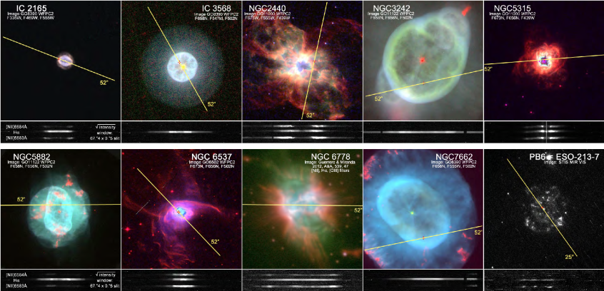
Figure 1: Slit positions and orientations (yellow lines) on multi-filter images of our target PNe. The image of PB6 is an exception: it is the pointing exposure for the STIS observations. Portions of the G750M STIS spectrum are shown below each image. They show the emission line intensity distributions of the H$\rm\alpha$ and [N II] lines that are characteristic of emission lines in our STIS data. These “line profiles” are convolved in the dispersion direction by thermal broadening and internal motions within the nebulae. The actual slit location of NGC 2440 and NGC 7662 may have been offset by up to 2″ from the yellow line.

Figure 1 shows the final ten PNe chosen with the slit positions and orientations that were possible given HST observation windows and STIS safety constraints. The targets, coordinates and slit positions are given in Table 1. Most images were obtained with HST/WFPC2, in multiple passbands, and are presented in false-color. The images are all on the same spatial scale, with NE to the upper-left; see the figure caption for details. While in some cases we were able to include the central star in the slit, in others we were obligated to offset the slit by 5$\rm\arcsec$.

Because of the length of time involved in obtaining approval for the UV observations on an individual object by object basis, and the changes in some of the PN targets requiring the development of a new Phase II template, the first observations were not begun until 2012 January (NGC 3242) and completed a year later (2013 January; NGC 2440).

2.2 Observing Strategy

Our observing strategy was designed to achieve our primary science goals. The first goal was to obtain spectra of each target that covered the full, uninterrupted spectrum from UV through Optical (1150Å through 10,150Å), with sufficient resolution and sensitivity to derive nebular gas diagnostics and ionic abundances of all critical species. We achieved these goals by allocating a full orbit to obtaining UV spectra with the G140L, G230L, and G230M gratings, and two (or for the faintest targets, three) orbits to obtain optical spectra with the G430L, G430M, G750L, and G750M gratings. We balanced the need for good spectral resolution with the need for high sensitivity by using the 52$\rm\arcsec$X0.2$\rm\arcsec$ slit for the low-resolution gratings, and 52$\rm\arcsec\times 0.5\arcsec$ for the medium-resolution gratings. The higher resolution gratings allowed us to resolve blends of a few critical lines: C III] $\rm\lambda 1906$ from $\rm\lambda 1909$, H I $\rm\lambda 4341$ from [O III] $\rm\lambda 4363$; H I $\rm\lambda 6563$ from [N II] $\rm\lambda 6548$ and $\rm\lambda 6583$, [S III] $\rm\lambda 6312$ from [O I] $\rm\lambda 6300$, and [S II] $\rm\lambda 6716$ from $\rm\lambda 6731$.

The second goal was to make co-spatial observations (i.e., with identical positioning and orientation of the apertures) of each target in all spectra, in order to avoid highly uncertain corrections for ionization stratification. The brightness limits (local and global) for the STIS/MAMA detectors, the required segregation of MAMA and CCD exposures to separate visits, as well as the need to provide some flexibility in the final slit orientation for scheduling reasons, presented some challenges to the design of our observing program. All of our targets are spatially extended (a few are larger than the spatial extent of the slit for MAMA exposures), most nebulae have high UV surface brightness, and many of the central stars are very bright in the UV. On the other hand, the bright, central portion of these nebulae is precisely where we expected to detect changes in ionization with position (a third goal of our observing strategy). We therefore constrained our MAMA visits to occur close in time to the initial CCD visits, in order to use the same guide stars for the MAMA visit aquisition.

2.3 Data Acquisition

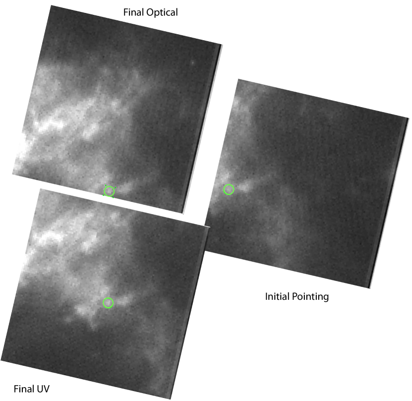
Figure 2: Acquisition images of NGC 2440 at the initial pointing, and the final positions for the UV and optical (northeast is in the upper-left). A green marker is superimposed on each image, indicating a nebular knot in common; the location of the knot indicates that the final location of the slit reference position in the optical-band lies almost directly south of the UV position by about 2.17″.

The observations were executed between 2012-Jan-15 and 2013-Jan-28, with the UV (MAMA) and optical (CCD) visits occurring within a few days of each other. See the observing log for this program in Table 2. Most observations were successful, except for a failure with the NUV exposures for NGC 6537 (which was subsequently repeated some weeks later), and an acquisition failure for NGC 2440. All of the exposures for NGC 2440 were executed, but our examination of the acquisition images shows that the UV and Optical slit positions were not perfectly co-spatial. We analyzed, with the help of ST ScI staff, the failed acquisition sequence for NGC 2440. The acquisitions begin with a short exposure of a 5″$\rm\times 5\arcsec$ field within STIS 50CCD aperture at the initial spacecraft pointing. The next step, locating the brightest feature in the field, failed for both the UV and CCD visits. The subsequent offset in each visit placed the final slit position for the UV and optical-band exposures in different locations. Figure 2 shows the acquisition images at the initial pointing, and the final positions for the UV and Optical (northeast is in the upper-left). A green marker is superimposed on each image, indicating a nebular knot in common; the location of the knot indicates that the final location of the slit reference position in the optical-band lies almost directly south of the UV position by about 2.17″. In a forthcoming paper we will analyze the emission line profiles for the brighter nebulae in our sample. Our initial profile analysis for NGC 2440 suggests that the ionization stratification (and, perhaps, extinction) varies significantly with position, so that the ionic abundance analysis involving UV emission lines may not correspond well to that of the optical lines. While the emission line fluxes are presented here (see Sect. 2.4), it must be kept in mind that the UV and optical data are from different regions in the nebulae that may have somewhat different ionization.

2.4 Data Reduction and Spectral Extractions

The data were reduced and calibrated using the CALSTIS v2.36 pipeline (ca. 2011-May-27). The processing depends upon the detector in use (MAMA or CCD), and is described in detail by Bostroem & Proffitt (2011). Briefly, the processing includes overscan and bias correction (CCD only) or re-binning by a factor of 2 (MAMA only), bad pixel flagging, dark and flat-field corrections, fringe correction (CCD G750 only), calibrations of the world coordinate system (wavelength and spatial extent of the slit), flux calibration (see Holland, et al., 2014, and references therein), and geometric rectification. The pipeline is capable of producing a variety of calibrated data products, but our spatially extended targets require custom spectral extraction from the calibrated, two-dimensional spectrograms: the *_sx2.fits files (hereafter, SX2). These products include a science array, a bit-encoded mask array that records detector or processing anomalies at the pixel level, and a variance array.

For each PN we examined the SX2 files and the emission profiles of the brighter lines from all gratings to determine the optimal spatial region for extraction. Since the spatial scales differ between the MAMA and CCD detectors (and between some CCD gratings), we developed a utility to extract regions that are spatially matched, rounded to the nearest whole pixel, for all gratings for a given target. The extraction regions are given in the last column of Table 1, in arcseconds relative to the slit reference position. Note that the spatial extent of the extraction regions is rather large, spanning nearly the entire extent of the target, so rounding the extremes to integral pixels has no significant effect on the relative fluxes between gratings. The extractions to one dimension were derived from the SX2 images by averaging pixel values at each wavelength (column) over the specified spatial range, normalizing by the extraction area in pixels, and converting from surface brightness to flux density. All pixels marked as bad in the pixel mask were excluded except for those flagged as affected by flat-field blemishes, noisy background, and excessive dark rate, as long as no other flags applied. While ignoring these flags adds some additional uncertainty to the average value, the final average is usually dominated by well exposed pixels where these pathologies are unimportant. In rare instances (at the edge of the MAMA detectors) all pixels were flagged as bad, so the average flux at such wavelengths was set to zero. No background subtraction was performed at this stage. In cases where the slit was positioned close to or included the central star, special care was taken to minimize stellar contamination of the nebular spectrum. In the end, signal-to-noise considerations and scattering of the starlight by dust in some nebulae compelled us to accept some stellar light in the cases of IC 3568, NGC 5315, and NGC 5882.

2.5 Measurements

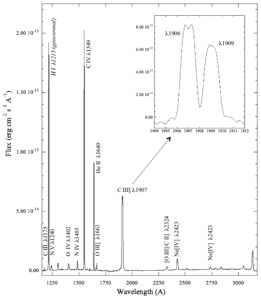
Figure 3: Spectrum of IC 2165 over the UV wavelength range. Numerous emission lines are identified. The inset shows an enlarged view of the closely-spaced lines of C III] $\rm\lambda\lambda$ 1906,1909.

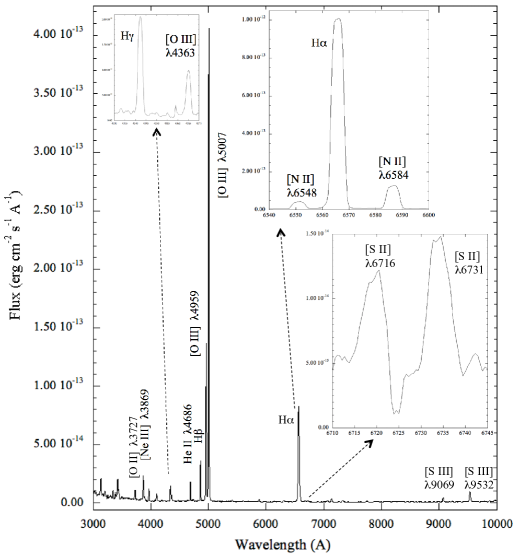
Figure 4: Spectrum of IC 2165 over the optical wavelength range. Numerous emission lines are identified. The insets show enlarged views of three line complexes: [S II] $\rm\lambda\lambda$6716,6731; [N II] $\rm\lambda\lambda$ 6548,6584 straddling H$\rm\alpha$; and the region from H$\rm\gamma$ to [O III] $\rm\lambda$4363.

Emission-line fluxes were measured using the IRAF splot package. Most lines were observed only in the L gratings. Regions with important closely-spaced lines were also observed with the medium-resolution M gratings, through a wider slit: see Table 2. Measurements of the better-resolved M spectra yielded ratios for these lines, which were then used to apportion the summed flux measured on the L spectra. For weak lines detected only in the M spectra, the measured flux was multiplied by 2.5, the ratio of the L and M slit widths. Figures 3 and 4 show UV and optical spactrograms, respectively, for IC 2165 as examples of the data quality and spectral range. Numerous emission lines are identified; inset graphs show enlargements of some line complexes.

Lines intensities are given in Tables 3 and 4, normalized to F(H$\rm\beta$)=100. The columns are, in order: the wavelength of the emission line; the line identification by ion; f($\rm\lambda)$, the value of the reddening function at that wavelength; F($\rm\lambda$), the observed line flux; and I($\rm\lambda$), the corrected line intensity with its uncertainty. Stellar and stellar+nebular composite lines are noted, as are lines that may be affected by artifacts in the 2D spectrogram. At the end of the table are, for each nebula, the calculated value of c, the logarithmic reddening parameter; the expected, zero reddening ratio of F(H$\rm\alpha$)/F(H$\rm\beta$) for the derived nebular temperature (from T[O III]) and density (usually from N[S II]); and the observed F(H$\rm\beta$) through the extraction window. Note that we give the line intensities for NGC 2440 in two columns: one for the UV (MAMA) spectra and another for the optical (CCD) spectra. Although the regions are in principle distinct, we normalize the fluxes to F(H$\rm\beta$) as measured in the optical, and determine the diagnostics and abundances as if they were from the same location (see §3.2.3); we call out the potential for problems in the results below.

Uncertainties were estimated in the following way. For each line, we obtained the RMS continuum value on either side (the m key in splot); sometimes only one side was amenable for measurement. We took the average RMS of the two sides and multiplied it by the line FWHM (k key or via deblending option in splot) to obtain the line flux uncertainty. The emission-line fluxes along with their uncertainties constitute the input for our abundance determinations using ELSA, our 5-level atom code (Johnson et al., 2006). ELSA propagates the uncertainties though the calculations, including the intensities, diagnostics and abundances. The first step in the analysis is to generate a table of line intensities that have been corrected for interstellar reddening and for contamination of the hydrogen Balmer lines by coincident recombination lines of He⁺⁺. In addition, ELSA can disentangle some unresolved line blends (here, [Ne III] $\rm\lambda$3968 and H$\rm\epsilon$ $\rm\lambda$3970) when one or both of the lines has a known ratio to another measured line. We corrected for the effects of reddening using the function of Savage & Mathis (1979) in the optical region, and Seaton (1979) in the ultraviolet. Details of the analysis using ELSA are described in Milingo et al. (2010).

A few very weak emission lines were noted in three objects that we were unable to identify. These are noted in Table 5 by wavelength and the nebula in which they were found; the intensities were comparable to the noise in the surrounding continuum. Though weak, the lines appear in the SX2 images to have profiles similar to other, well exposed nebular lines rather than artifacts (e.g., hot pixels or charge trails). We note them here in the hope that future investigations may be able to make use of them.

3 Results

3.1 Plasma Diagnostics and Abundances

We present the plasma diagnostics in Table 6. The [O III] temperature is derived from the I($\rm\lambda 4343$)/I($\rm\lambda 5007$) ratio. Where available, the [N II] temperature is derived from the I($\rm\lambda 5755$)/I($\rm\lambda 6584$) ratio; otherwise, based on previous work (Kwitter & Henry, 2001): if He II $\rm\lambda 4686$ is detected, as it is in all PNe here, we adopt the carefully derived result from Kaler (1986) that applies under this condition, i.e., T[N II] = 10,300 K. If the required lines have been detected, we also report values of T[O II] from I($\rm\lambda 7323$)/I($\rm\lambda 3727$), but owing to the high uncertainty associated with these derived temperatures they are not used in any calculations. The T[S II] diagnostic from I($\rm\lambda[4068+4076]$)/I($\rm\lambda[6717+6731]$) failed to give reliable results because the emission is quite weak, and the $\rm\lambda 4068+4076$ doublet is potentially blended with weak recombination lines. If the [S III] lines $\rm\lambda 6312$ and one of $\rm\lambda 9069$ or $\rm\lambda 9532$ are available, T[S III] is calculated and, if it is within 5000 K of T[O III], we use it to derive the abundances of S⁺² and Cl⁺². In general, T[O III] is used for both helium ions and for other ions in states +2 or above; T[N II] is used for the other singly-ionized species. Electron densities are calculated using ratios of [S II] I($\rm\lambda 6717$)/I($\rm\lambda 6731$) and C III] I($\rm\lambda 1909$)/I($\rm\lambda 1906$). If only one density diagnostic is available, it is used for all calculations. If both are available, N[S II] is used to calculate abundances of singly-ionized species, and N[C III] is used for the higher-ionization species.

Ionic abundances derived using ELSA are given in Table 7. The first column lists the ion and wavelength used to calculate the values in each row; the adopted value for the ionic abundance corresponds to the mean of all the observed lines of that ion, weighted by raw observed flux, and is used in subsequent calculations. Measured lines contaminated by stellar emission (indicated in Tables 3 and 4) are excluded from further analysis. Values of the ionization correction factor (ICF) that was derived to compute total abundances are shown at the end of each ion listing; these have been calculated in ELSA as described in Kwitter & Henry (2001), except for carbon, which was not studied in that paper. Here we use the following:

$$\sf\rm C/H=\frac{C^{++}}{H^{+}}\times ICF(C)$$

where

$$\sf\rm ICF(C)=\frac{(O^{+}+O^{++})}{O^{++}}\times\frac{(He^{+}+He^{++})}{He^{+}}$$

The total elemental abundances are shown in Table 8. For C- and N-related parameters, we show both the values derived using ICFs and those obtained by summing abundances of observed ions. Note that abundances of O, Ne, S, and Ar presented here are ICF values. The last two columns give values for the Sun (Asplund et al., 2009) and Orion (Esteban et al., 2004).

3.2 Individual Nebulae

Here we discuss the abundance results for eight of the 10 PNe we observed. NGC 6537 and NGC 6778 are not included since the low S/N of the STIS data prevented any meaningful homogeneous abundance analysis. The emission line intensities for these excluded objects, presented in Table 4, should inform future investigators of the stronger UV emission lines, and of the approximate scaling from the UV to optical band. Our spectrograms for PB 6 are also weakly exposed, but we are able to combine the UV emission lines with published spectra to confirm the very high enrichments of He, C, and N noted in the literature. Photoionization models of these eight PNe will be presented in a forthcoming paper.

We note again that our data are strictly co-spatial (except for NGC 2440), meaning that we are sampling the same region in each PN across the entire observed spectral range. The co-spatial results are thus free of any need for aperture size or placement corrections whose values can be difficult to calculate and whose effects on the final abundances almost impossible to assess. All calculated elemental abundances are listed in Table 8; we only discuss CNO abundances here. Table 9 shows our CNO abundances and those of various other authors with whom we compare below. All of our O abundances come from ICF calculations. We compare our summed values for C and N where available (for some PNe we had to exclude lines compromised by stellar emission, which we discuss in more detail below). We derived upper limits for key undetected ions and note their potential contribution. We also compare the abundances derived with the ICF values, and comment on any discrepancies with the sums. Note that the ICF values for PNe where the value of T[N II] is assumed are particularly uncertain; however, our conclusions are based on the summed-ion results, which are unaffected by this uncertainty. As mentioned above, T[N II] is used only to calculate ionic abundances for singly-ionized species, which are generally minor contributors to the total C and N abundances. Further, comparison of results using our default T[N II] of 10,300 K from Kaler (1986) with the recipe from Kingsburgh & Barlow (1994) yields insignificant differences in the contribution of N+ to the total N abundance.

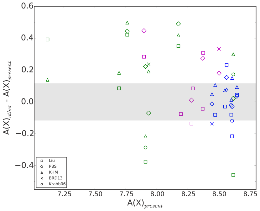
Figure 5: Difference between published log abundances and those of this study, as a function of our log abundance for the elements. Elements X are color-coded C: magenta, N: green, and O: blue. Published abundances are from Liu and collaborators (squares): Liu et al. (2004a, b); Tsamis et al. (2003); Pottasch and collaborators (diamonds): Pottasch et al. (2002); Bernard-Salas et al. (2002); Pottasch & Bernard-Salas (2008); Pottasch et al. (2004); Bohigas et al. (2013); Kwitter and collaborators (triangles): Milingo et al. (2002); Kwitter et al. (2003); Henry et al. (2004); Milingo et al. (2010); Dufour and collaborators (stars): Bohigas et al. (2013); and Krabb (circles): Krabbe & Copetti (2006). Grey band shows agreement within 30%.

In the following subsections where we compare our CNO abundances for each nebula in detail with those from other authors, it is worth noting at the outset the level of agreement among all authors for all nebulae, shown in Fig. 5. Individual research groups are denoted with the same symbol, as they tend to use the same methodology, the same atomic parameters, and similar observing technique. The elements are differentiated by symbol color. The figure shows that the agreement among all authors for O abundance is generally good, within 30% for most cases. The agreement for C and N is much poorer, with many deviations approaching a factor of a few. In an exhaustive comparison of abundances derived for Magellanic Cloud PNe, Shaw et al. (2010) noted several reasons why abundances of the same object often differ from author to author. In some cases the differences in Fig. 5 can be attributed to other authors’ use of fluxes obtained with different apertures; for nebulae with significant ionization stratification such discrepancies are worrisome. Discrepancies can also arise from the use of different atomic parameters, different extinction constants, different techniques (e.g., the adoption of different T_e or N_e for different ions), or flawed observing techniques or data calibration. Note that discrepancies in any datum or derived parameter propagates downstream to the derivation of the final elemental abundances. This is a particular problem for abundances derived with ICF methods. In the comparisons below, we attempted to select data from the literature that represent the best available for these well-observed nebulae.

3.2.1 IC 2165

This object has a bright, angularly small ($\rm\sim 7$″) core and a faint, extended halo (Corradi et al., 2003). There is significant ionization stratification with position along the slit, with most of the emission from very low ionization species such as O⁺, N⁺, and S⁺ located on the periphery (see Fig. 1). Our ICF and summed ion abundances agree very well for both C (12% difference) and N (7% difference), indicating that the ICF method is doing a good job of accounting for ionization states that would be missed had only optical data been available. Kwitter et al. (2003) observed IC 2165 (optical only); their O/H value is within $\rm\sim$$\rm 12\%$ of ours. Their N/H value is $\rm\sim$60% larger than our N/H, due to their comparably greater ICF(N) stemming from a smaller derived O$\rm{}^{+}/H^{+}$. They did not observe C.

Pottasch et al. (2004) reported abundances for IC 2165 derived from combining IUE, ground-based optical (primarily) from Hyung (1994), and ISO fluxes. Both the IUE and ISO apertures are larger than this nebula, but the ground-based data were averages from multiple observers, where some spectra were obtained through smaller apertures placed at different nebular locations. The optical slit spectra from Hyung (1994), which was only 4″ long, weighted the center of the nebular emission more heavily and hence missed much of the [O II] $\rm\lambda 3727$ and [N II] $\rm\lambda 6583$ emission. Their O abundance is very close to ours, but this is somewhat of a coincidence: they derived a much lower O⁺ abundance because of a lower observed I(3727), but they derive a significant O⁺³ abundance from the IR $\rm 25.8~{}\mu$m line. We observed O IV] UV emission, but we used ICF(O) to account for O⁺³ and higher ionization stages. Their N/H is $\rm\sim$17% less than ours, mostly because their I(6584) was much lower than ours. Finally, their C/H is $\rm\sim$50% more than our value, in spite of very similar intensities for the relevant emission lines: the discrepancy may come from either or both of different atomic parameters or their adoption of somewhat different T_e values.

Most recently, IC 2165 was observed by Bohigas et al. (2013) (optical only), who obtained optical echelle spectroscopy of the inner 22″$\rm\times 27$″ region. The much narrower STIS slit, as shown in Fig. 1, passes through the long axis of the nebula, and does not sample as large a variety of environments. Comparing with their results derived by the “standard” method, our O abundance is 37% larger than theirs, due primarily to our higher O⁺/H⁺. Our value and their value for N⁺/H⁺ are within $\rm\sim$$\rm 12\%$, but as a result of their larger ICF(N), our N/H abundance is only $\rm\sim$55% of theirs. Their C abundance, derived exclusively from permitted lines, is almost double ours. The He abundance (He/H=0.106), coupled with low N/O ($\rm\sim$0.3), corroborates the conclusion that IC 2165 originates from a progenitor not much more massive than $\rm\sim$2M_⊙ (e.g., Bohigas et al. 2013). The C/O ratio ($\rm\sim 1.2$) is larger than the solar value, perhaps indicative of some C production.

3.2.2 IC 3568

This object is $\rm\sim 18$″ in size, with a bright inner core of $\rm\sim 7$″; there is little ionization stratification, however the FUV spectrum shows stellar P-Cyg profiles in N V and C IV. Our calculations of ICF and summed-ion abundances for C agree to within 6%, giving confidence in the numbers. Many of our spectrograms for this object were less than optimally exposed: we determined only upper limits for nebular UV N lines, for example. Henry et al. (2004) derived abundances for IC 3568 from optical spectra; their N/H and O/H are 37% and 28% higher, respectively. Liu et al. (2004a, b) also observed IC 3568 and calculated CNO abundances combining IUE and ISO data with optical recombination lines and with collisionally-excited lines. We compare our results with their collisionally-excited line results and find that the C/H and O/H agree within 25%. However, our N/H using ICF(N) is only 40% of theirs, despite our N⁺/H⁺ being twice as large. The difference is due to their inclusion of N III] $\rm\lambda$1750 from IUE data (we have only upper limits from our STIS data) to derive N⁺⁺/H⁺. We detected only the N⁺ ion which had a rather large ICF(N) of 33.3, but our sum of N⁺ and the upper limit to N⁺² agrees well with that of Liu et al. (2004a, b). Our O abundance agrees within $\rm\sim$25% to that of Henry et al. (2004). Based on our results, He/H (0.118) is slightly above solar, C/O ($\rm\sim$0.5) is solar, and N/O (0.04) is slightly sub-solar.

3.2.3 NGC 2440

This object is angularly large ($\rm 74\arcsec\times 42\arcsec$) with highly stratified ionization. Our results for NGC 2440 are uncertain to the extent that the slit positions for the UV and optical observations sampled different locations (see § 2.3). Based on the STIS data, the ICF abundances of C and N are 60% higher and 2.3 times higher than the ion-sum values, respectively. Both O⁺ and O⁺⁺ are well measured in our spectra, as are He⁺ and He⁺⁺, so the ICF values should be accurate. It may be that the spatial offset of the UV and optical spectra, described above, sampled sufficiently different regions that these two results are not directly comparable.

NGC 2440 has been observed by many authors, including Bernard-Salas et al. (2002) who combined ISO IR data with IUE UV data and previously-published optical data; and Tsamis et al. (2003), who observed the entire nebula and combined their optical data with IUE data; Kwitter et al. (2003) and Krabbe & Copetti (2006) observed in the optical only. Our ion-summed C abundance is 82% of what Tsamis et al. (2003) reports, and only 28% of values reported by Kwitter et al. (2003) and Bernard-Salas et al. (2002). Our ion-summed N abundance is $\rm\sim$50% of Kwitter et al. (2003)’s, $\rm\sim$68% of Krabbe & Copetti (2006)’s, and $\rm\sim$95% of Bernard-Salas et al. (2002)’s, but 2.8 times that of Tsamis et al. (2003). These last authors did not detect any N⁺, so their entire N abundance is based on IUE lines. Inspection of their ionic abundances reveals that their values of N⁺⁺, N⁺³, and N⁺⁴ are systematically 2–5 times lower than ours. The source of the discrepancy may lie in our mis-matched apertures. However, since this nebula is larger than the ISO and IUE apertures and is highly stratified, the discrepancy could equally well indicate a problem with matching the satellite data to those from the ground-based spectra. The He/H ratio in NGC 2440 (0.127) and the N/O ratio, whether ICF (1.6) or summed-ion (1.0) are both greater than solar and suggest that the progenitor of this PN was relatively high mass.

3.2.4 NGC 3242

This object is angularly large, with a core of $\rm 16\arcsec\times 26\arcsec$, surrounded by a faint shell of about $\rm 40\arcsec\times 35\arcsec$ (Corradi et al., 2003). Within the bright inner core there is moderate ionization stratification. Our ICF and summed-ion results for NGC 3242 are quite disparate: C(ICF) $\rm=1.5\times$C(sum) and N(ICF) $\rm=0.5\times$N(sum). Milingo et al. (2002) observed NGC 3242 in the optical only, as did Krabbe & Copetti (2006). Pottasch & Bernard-Salas (2008) combined ISO IR data with IUE UV data and previously-published ground-based optical data. Tsamis et al. (2003) observed the entire nebula and combined their data with IUE data.

All of these authors’ O abundances agree with ours to $\rm\sim 30$%. The C abundance from Tsamis et al. (2003) is half of our ICF value and 73% of our summed-ion value; they used only C III] $\rm\lambda$1909, and did not include C IV $\rm\lambda$1549 or C II] $\rm\lambda$2324. The C abundance (and also the C⁺² and C⁺³ ionic abundances) from Pottasch & Bernard-Salas (2008) agrees perfectly with our summed-ion value in spite of significantly different intensities for the lines used to derive the ionic abundances. Their C abundance is 70% of our ICF value. Our ICF-based N abundance agrees to $\rm\sim$20% with those of Krabbe & Copetti (2006), Tsamis et al. (2003), and Milingo et al. (2002), but is three times lower than that of Pottasch & Bernard-Salas (2008). Since our summed-ion N value is twice as high as the ICF value, the agreement just described suffers by a factor of two. The He/H ratio in NGC 3242 is slightly above solar (0.115), the N/O is 0.1 (ICF) or 0.2 (sum).

3.2.5 NGC 5315

This object is angularly small ($\rm\sim 15$″), with modest ionization stratification, but there are very bright stellar emission lines. This analysis for this PN is problematic: the S/N is not as high as needed for a robust abundance analysis, since we had to avoid much of the spatial extent of the nebula in order to exclude a substantial contribution of scattered stellar P-Cyg emission to the nebular emission. As a result, we have not used any He II lines in the abundance analysis; the ICF values in Table 7 should therefore be viewed as lower limits. NGC 5315 was observed previously in the optical by Milingo et al. (2010) and by Tsamis et al. (2003) who observed the entire nebula, and combined their data with IUE data; Pottasch et al. (2002) combined their IR observations with IUE and previously-published optical data. These other investigators derived O abundances $\rm\sim$18-70% larger than ours. Their N abundances are within 30% of our N(ICF) values and 2-3 times our summed-ion N abundance. Our ICF and summed-ion C abundances are in excellent agreement, and within $\rm\sim$10% of the Tsamis et al. (2003) value. Despite Pottasch et al. (2002) deriving ionic abundances for C⁺ and C⁺⁺ similar to ours, their application of an ICF yields a C abundance roughly twice ours. Milingo et al. (2010), using only the C⁺⁺ permitted line at $\rm\lambda$4267, derive a C abundances 3.5 times ours. The He/H ratio (0.132) and the N/O ratio (1.1, using the ICF value are clearly greater than the solar values.

3.2.6 NGC 5882

This nebula is intermediate in size (Corradi et al., 2000) with a bright, elliptical inner shell ($\rm 11\arcsec\times 6\arcsec$), surrounded by a spherical outer shell (15″); it has substantial ionization stratification. Scattered stellar light was an issue in the STIS observations, reducing the region of the slit usable for nebular analysis, with the higher-ionization lines of N and C being of stellar origin. NGC 5882 was observed in the optical by Kwitter et al. (2003) and by Tsamis et al. (2003), who observed the entire nebula, and combined their data with IUE data. Pottasch et al. (2004) observed the full spatial extent of the nebula with ISO in the IR, and combined their observations with IUE data in the UV and previously-published, ground-based optical data (primarily from Tsamis et al. (2003)). All of the O abundances agree with ours to 25%. The N abundances from these authors agree with each other to 20% but are 2–3 times ours, which is based solely on optical N⁺/H⁺ and an ICF(N) of $\rm\sim$33. Our upper limit to the N III] $\rm\lambda 1750$ emission is less than half that of Pottasch et al. (2004), but their N⁺² abundance (the dominant ionization stage), derived from the $\rm 57\mu$m emission line, is larger than ours by a factor of 5.

Tsamis et al. (2003) and Pottasch et al. (2004) derived C abundances from C III] $\rm\lambda$1909 in the same IUE data, calculating similar C⁺⁺/H⁺ ratios, about twice what we derive from the co-spatial STIS data. This, together with the use of different ICF values, produces total C abundance that are 75% larger and 2.5 times larger than ours, respectively. The He/H (0.11) and N/O (0.13) in NGC 5882 is roughly solar

3.2.7 NGC 7662

This nebula is moderately large, with a bright shell $\rm\sim 30$″ in diameter (Corradi et al., 2003), and considerable ionization stratification. Our STIS data show that the ICF values and summed-ion values agree very well, within $\rm\sim$$\rm 1\%$ for C and $\rm\sim$$\rm 14\%$ for N, indicating that, as in IC 2165, the ICF method is yielding reliable abundances. NGC 7662 has been observed by Kwitter et al. (2003) in the optical, and by Liu et al. (2004a, b) who combined their data with IUE UV data. The O abundances agree well, within 20%. Our C abundance is only half that found by Liu et al. (2004a, b), despite our ionic abundances agreeing with theirs to within 30%. The difference is that they apply an ICF (=2.0) to their ion sum. Our N abundance is $\rm\sim$65% of those derived by Liu et al. (2004a, b) and Kwitter et al. (2003). The difference with Liu et al. (2004a, b) appears mainly to be their higher N⁺⁴ because of a higher observed N V $\rm\lambda 1240$ emission, which is likely the result of scaling the fluxes from the IUE large aperture to their 1″ optical slit. Our ICF N abundance hinges on weak O⁺/H⁺, but the good agreement with the ion sum implies that the ICF itself is not the reason. The He/H (0.122) is higher than solar but the N/O ratio (0.13) very close to solar,

3.2.8 PB 6

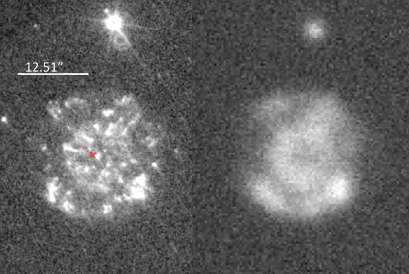
Figure 6: Images of PB 6 obtained with STIS in white light through the F28X50LP aperture (left), where the emission is dominated by H$\rm\alpha$ and [N II], compared to a ground-based image in [O III] $\rm\lambda 5007$ obtained by one of us (R.L.M.C.) with the EFOSC2 camera on the 3.5m NTT ESO telescope under 1.5″ seeing conditions. The images are oriented with North up and East to the left; the bar in the upper left provides the scale. Note that the apparent double-shell structure in the NTT image is resolved into a complex set of knots in the higher resolution STIS image.

This object is a small ($\rm 14.0\arcsec\times 12.5\arcsec$), clumpy nebula with a bright, [WC] central star, as shown in Fig. 6. A ground-based image in [O III] obtained by one of us (R.L.M.C.; included in Fig. 6) shows what appear to be two concentric, nearly circular shells, but the higher-resolution STIS image resolves the structure into a complex of knots. Some of the knots appear to have a linear, or cometary structure oriented away from the central star, not unlike those seen in Abell 30 and Abell 78 (Fang et al., 2014). The He/H, C/O, and N/O ratios for this nebula have been reported to be extraordinarily high. Kaler et al. (1991) first noted the presence of very strong O VI emission in the optical, and strong stellar emission is apparent in our UV and optical spectrograms as well.

Our spectrograms are too weakly exposed to derive robust abundances, or even reliable physical diagnostics. García-Rojas, Peña & Peimbert (2009, hereafter GRPP) obtained deep optical spectra in order to use faint recombination lines to derive abundances. They derived values for T_e and N_e from CELs which are consistent with other published values, and found from ORLs high enrichments of He, C, and N. Our emission line intensities, uncertain as they are, are consistent with those reported in GRPP apart from our detection of a stronger [N II] $\rm\lambda 6583$ flux. Our spectrograms, and the two zones within PB 6 analyzed by GRPP, indicate that the ionization is not strongly stratified within this nebula. We used the optical intensities from GRPP and our UV data to compute the abundances from CELs using ELSA, in order to compare techniques (in spite of the mis-matched apertures). We find that the He and CNO abundances derived in this way generally agree with those from GRPP, although the strong observed (but uncertain) C⁺³ abundance from our UV spectrum suggests that C could be even higher. Keller, Bianchi, & Maciel (2014) modelled the central star spectrum to derive T$\rm{}_{eff}=165,000$ K and $\rm log(L/L\sun)=3.43$, using data from FUSE and our UV spectrograms from STIS; their results are also consistent with the high ionization of this nebula.

4 Discussion

It is well known that PNe exhibit a wide variety of ionization structures. This is especially true of PNe that are not fully ionized, where the ionization is often a complicated function of position within the nebula. Unless spectra can be obtained that intercept the light from the full spatial extent of the nebula (which is usually achieved only for angularly small PNe, such as those in external galaxies), the derivation of nebular conditions and elemental abundances must of necessity sample a limited, possibly small volume within the nebulosity. We have shown here (as many before us have) that the most reliable elemental abundances are derived by observing a full range of ionic species, which requires spectra spanning at least the UV through optical bands, at high S/N and moderate-to-high spectral resolution. Often this requires the use of multiple spectrographs on different platforms. We believe the most accurate abundances are derived when all spectroscopic apertures sample identical three-dimensional volumes of the nebulosity. Indeed, for nebulae with stratified ionization, co-spatial apertures are essential for deriving consistent plasma diagnostics, ICFs, and elemental abundances. We have shown in some key cases (including IC 2165, NGC 3242, and NGC5882) that the primary reason for the large difference between our derived ionic and elemental abundances, and those in the literature (up to a factor of a few: see Fig. 5), is the mis-application of data from spatially distinct regions. It is our assertion, to be explored further in forthcoming papers, that to reach the level of precision necessary to discriminate between modern, competing theories of elemental yields in post-AGB stars, it simply will not suffice to scale or select emission line intensities from one nebular region and to transplant them to another, spatially distinct region.

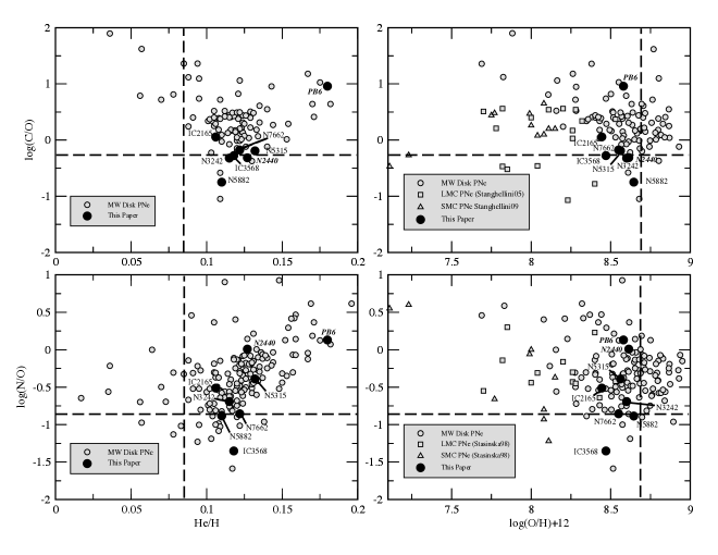
Figure 7: Left panels: log(C/O) and log(N/O) versus He/H, respectively. Program objects are represented by large filled circles, while data from the KH database are indicated with small gray circles. Right panels: Same as left panels but with log(O/H)+12 as the independent variable. Additional data for the LMC and SMC have also been included from papers cited in the legends. Bold dashed lines indicate solar values. Program objects are identified in each panel, where names of Type I PNe appear in italics. Note that the abundances for PB 6 are taken from GRPP.

Figure 7 graphically displays the summed abundance results given in Table 8 for the program PNe discussed in the previous section (large filled circles). Because our optical line measurements for PB6 proved to be unreliable (see §3.2), the positions for PB 6 in all four panels were determined using abundances from Peña et al. (1998). Despite the fact that our data for PB6 are less than satisfactory, we decided to include it in Fig. 7 because it harbors a [WC] central star, it is a Type I PN, and possesses an inordinately high nebular He abundance, making it an interesting object to compare with the other sample members. The left-hand panels show log(C/O) and log(N/O) versus He/H, while the right-hand panels do so for the same dependent variables against log(O/H)+12. To provide a comparison with a larger sample, the small, gray dots show abundance ratios from the KH database. In the right-hand panels we have also added results from Stanghellini et al. (2005, 2009) and Stasińska et al. (1998) for the LMC and SMC in order to extend the metallicity range to lower values. Within our sample of eight PNe, Type I objects are identified with italicized font, while names of non-Type I PNe are shown with regular font. The bold dashed lines show solar values from Asplund et al. (2009).

The right-hand panels demonstrate that there is no clear trend in either C/O or N/O with respect to the metallicity range of objects observed, as gauged by log(O/H)+12. This is in contrast to what is anticipated by recent model results. Post-AGB stellar models and the consequent PN abundance predictions published by Karakas (2010) for low stellar metallicity progenitor stars [e.g. 0.004 (SMC), 0.008 (LMC), corresponding respectively to 8.00 and 8.30 on the horizontal scale) with birth masses below 4 M_⊙ suggest that C/O should be noticeably greater than in the case of the solar-like metallicities characteristic of our program objects. Similarly, above this mass threshold, where hot bottom burning (HBB) converts dredged up C into primary N, N/O should be greater at low metallicities than at levels closer to solar. HBB most likely occurred during the late evolutionary stages of progenitors of IC 2165, NGC 2440, NGC 5315 and PB6 since their N/O ratios are significantly higher than those of the remaining sample PNe. Note that the first three members of this group are not outstanding in terms of their C/O or He/H abundances. All of our objects were chosen so as to have near-solar metallicities, and the range of that parameter among them is rather small. Thus the lack of a metallicity trend among them in either C/O or N/O is not surprising. However, even with the extension of the sampled metallicity range provided especially by the LMC and SMC objects, the model-predicted trend remains elusive. This is perhaps due to the large amount of scatter observed among objects of similar metallicity (see below).

Three of our eight objects (IC 2165, NGC 7662 and PB6) show C/O ratios which are greater than or equal to the solar value. In the cases of IC 2165 and PB6 the C/O ratio exceeds unity, suggesting that their progenitor AGB stars experienced significant third dredge-up during which fresh carbon produced by triple-alpha processing was brought up by convection into the stellar atmosphere from the He-burning shell located just above the C-O core of the remnant star.

The left-hand panels in Fig. 7 show the distribution of our program objects and the KH database objects in the log(C/O) and log(N/O)-He/H planes. Note the suggestion of a positive correlation between log(N/O) and He/H. This has been noticed many times before; one such example is included in the extensive review by Kaler (1985). This positive behavior is predicted by stellar evolution models (cf. Marigo, 2001; Karakas, 2010) and is fundamentally associated with a positive correlation between N/O and stellar mass. In a followup paper to this one we explore more closely the relation between the progenitor masses and the abundance results of the present work.

Peimbert & Torres-Peimbert (1983) referred to those PNe in which He/H$\rm\geq$0.125 and log(N/O)$\rm\geq$-0.30 as Type I objects, while PNe below these boundaries were considered to be non-Type Is. By these criteria then, NGC 2440 and PB6 are Type I objects, while the other six are non-Type Is. PB6’s Type I membership is confirmed by Peña et al. (1998), who find He/H = 0.17 and log(N/O) = 0.14.

The PNe with supersolar N/O have several other interesting properties that distinguish them from those PNe with solar or subsolar N/O. The most dramatic are their morphologies. Members of the latter group are all elliptical in outline with very conspicuous central cavities surrounded by thin bright rims and smooth and sharply bounded shells. None of the PNe with supersolar N/O have similar morphologies. Either they are bipolar (NGC 2440), clumpy (PB6), or elliptical with central cavities but no thin rim (IC2165 and NGC5315). NGC5315 is also a serendipitously discovered diffuse x-ray source (Kastner et al., 2008). Thin rims are the result of relatively gentle expansions of the hot cavities within them, whereas fractured rims are the result of instabilities induced by rapid cavity expansion at high pressure (Toalá & Arthur, 2014). We note that as a rule, the nebular expansion velocities of PNe with [WC] nuclei are well above average (Górny & Stasińska, 1995), again suggesting a high degree of momentum transfer from stellar winds during their evolutions.

The central stars of PNe with supersolar N/O also stand out from the others. NGC 5315 and PB6 have early-type WC or WO nuclei [see Kaler et al. (1991), Peña et al. (1998) and Acker & Neiner (2003)]. The central star of NGC 2440 is the hottest known (Heap & Hintzen, 1990). NGC 5315 and NGC 2440 have probably evolved from relatively massive progenitors whose mass loss rates in radiation-driven winds are or have been very strong. The central star of IC 2165, whose progenitor is probably not as massive as these, may simply be at a high-temperature stage in its evolution.

Finally, an obvious characteristic in each of the four panels in Fig. 7 is the large amount of point-to-point scatter in C/O, N/O and He/H; scatter is present in all of the individual samples included in the figures. The sizes of the uncertainties (not indicated here to avoid visual confusion, but see Table 8) are dwarfed by the sizable scatter exhibited in each panel. Therefore, the scatter is very likely real and indicative of the wide range of chemical inhomogeneity in the ISM from which these stars formed at various places and times within the galaxy and/or in the amount of atmospheric self-pollution that AGB stars experience during the final evolutionary stages of these stars.

5 Conclusions

The STIS long-slit data from this program are the first co-spatial spectra of extended Galactic PNe that span the UV and optical bands at sub-arcsecond spatial resolution. These new data enable a detailed and consistent analysis of abundance and physical properties of PNe using both UV and optical emission lines from identically sampled volumes. Compared to prior abundance analyses of past decades that studied only the major optical emission lines, or that used satellite UV with ground-based data from different nebular regions, this work offers new insights on UV-optical emission variations and permits corresponding analysis of nebular diagnostics in C and N lines from their major ions. This initial study of these STIS data touches only the top of the science inherent in the data, which will be analyzed in more detail in future papers. These HST data are now in the public domain and offer future investigators a new and, perhaps, historical insight into the spatial variations of UV-optical emission for modeling physical diagnostics across the extent of photoionized nebulae.

We conclude that the central stars and the morphological outcomes of nebular evolution of PNe with super-solar N/O are not typical of those of PNe with solar N/O. Although the evidence is somewhat circumstantial in this paper, there is every reason to suppose that the central stars of PNe with super-solar N/O have evolved from some of the most massive stars that are able to form PNe. This is one of the reasons that we selected a PN sample with a wide range of N/O at constant O/H. It is therefore peculiar that PNe with super-solar N/O show no signs of C/O anomalies. Perhaps this can be explained by the conversion of C to N during HBB, thereby increasing the N while holding C to a level close to its original one in the progenitor star. On the other hand, the abundance trends in our graphs plotted against He/H indicate that selecting PN samples based on He enrichment will be a fruitful approach to understanding CNO production.

Finally, the large amounts of scatter in the N/O and C/O ratios at roughly constant metallicity is much larger than can be explained by observational uncertainties, (although we cannot rule out the possibility of systematic errors in earlier publications because of, e.g. mis-matched apertures between spectra from multiple wavelength regimes). In fact the size of the scatter in our plot of C/O or N/O versus O/H dwarfs that observed among objects such as H II regions or main sequence stars, regardless of metallicity. We surmise that this situation may reflect the self-polluting nature of objects in the AGB stage of evolution or the chemical history of the Galactic ISM at the time and place when the stars formed (Matteucci, 2003)

Table 1: Slit Reference Positions and Extraction Regions

	Slit Reference Position
	RA	Dec	Offset from CS	Orient	Extract Bounds
Nebula	(J2000)	(J2000)	(arcsec)	(deg)	(arcsec)
IC2165	6 21 42.775	$\rm-12$ 59 12.96	0	68.650	$\rm-6.12:+4.68$
IC3568	12 33 07.340	+82 33 50.40	0.5 E	29.684	$\rm-2.52:-0.72$, $\rm+0.10:+1.62$
NGC2440	07 41 54.875	$\rm-18$ 12 29.97	Unknown	$\rm-13.350$	$\rm-9.80:+1.26$
NGC3242	10 24 46.107	$\rm-18$ 38 37.14	4.5 S	$\rm-77.350$	$\rm-7.20:+9.00$
NGC5315	13 53 56.980	$\rm-66$ 30 50.60	0.4 N	$\rm-85.345$	$\rm-1.80:+0.36$, $\rm+0.99:+3.60$
NGC5882	15 16 49.938	$\rm-45$ 38 57.19	0.0	$\rm-90.350$	$\rm-2.70:+2.52$
NGC6537	18 05 13.129	$\rm-19$ 50 34.62	0.0	$\rm-136.350$	$\rm-1.80:+2.16$
NGC6778	19 18 24.939	$\rm-01$ 35 47.41	0.0	89.651	$\rm-3.24:-0.36$, $\rm+0.72:-3.60$
NGC7662	23 25 53.600	+42 32 00.50	5.5 S	101.649	$\rm-2.52:+5.40$
PB6	10 13 15.989	$\rm-50$ 19 59.13	0.0	34.646	$\rm-6.48:-1.08$, $\rm+0.00:+6.12$

Table 2: Observing Log for GO 126000

			Grating/	Dispersion	Slit Width	TExp
Nebula	UT Date	Dataset	Cent. Wave	(Å/pix)	(arcsec)	(s)
IC2165	2012-Apr-28	OBRZ14010	G140L/1425	0.60	0.2	2280
		OBRZ14020	G230L/2376	1.58	0.2	1946
		OBRZ14030	G230M/1884	0.09	0.5	346
	2012-Apr-30	OBRZ13010	G430L/4300	2.75	0.2	360
		OBRZ13020	G430M/4451	0.28	0.5	210
		OBRZ13040	G750L/7751	4.92	0.2	360
		OBRZ13030	G750M/6581	0.56	0.5	165
IC3568	2012-Jul-15	OBRZ02010	G140L/1425	0.60	0.2	2624
		OBRZ02020	G230L/2376	1.58	0.2	2146
		OBRZ02030	G230M/1884	0.09	0.5	546
	2012-Jul-13	OBRZ01010	G430L/4300	2.75	0.2	456
		OBRZ01020	G430M/4451	0.28	0.5	276
		OBRZ01040	G750L/7751	4.92	0.2	426
		OBRZ01030	G750M/6581	0.56	0.5	276
NGC2440	2013-Jan-28	OBRZ27010	G140L/1425	0.60	0.2	2272
		OBRZ27020	G230L/2376	1.58	0.2	2862
		OBRZ27030	G230L/2376	1.58	0.2	882
		OBRZ27040	G230M/1884	0.09	0.5	504
		OBRZ27050	G230M/2338	0.09	0.5	564
	2013-Jan-21	OBRZ26010	G430L/4300	2.75	0.2	351
		OBRZ26020	G430M/4451	0.28	0.5	171
		OBRZ26040	G750L/7751	4.92	0.2	351
		OBRZ26030	G750M/6581	0.56	0.5	81
NGC3242	2012-Jan-21	OBRZ05010	G140L/1425	0.60	0.2	2242
		OBRZ05020	G230L/2376	1.58	0.2	1968
		OBRZ05030	G230M/1884	0.09	0.5	328
	2012-Jan-15	OBRZ04010	G430L/4300	2.75	0.2	360
		OBRZ04020	G430M/4451	0.28	0.5	189
		OBRZ04040	G750L/7751	4.92	0.2	330
		OBRZ04030	G750M/6581	0.56	0.5	180
NGC5315	2012-Feb-27	OBRZ17010	G140L/1425	0.60	0.2	2660
		OBRZ17020	G230L/2376	1.58	0.2	2122
		OBRZ17030	G230M/1884	0.09	0.5	522
	2012-Feb-26	OBRZ16010	G430L/4300	2.75	0.2	405
		OBRZ16020	G430M/4451	0.28	0.5	315
		OBRZ16040	G750L/7751	4.92	0.2	465
		OBRZ16030	G750M/6581	0.56	0.5	285
NGC5882	2012-Apr-21	OBRZ11010	G140L/1425	0.60	0.2	2328
		OBRZ11020	G230L/2376	1.58	0.2	2118
		OBRZ11030	G230M/1884	0.09	0.5	318
	2012-Apr-19	OBRZ10010	G430L/4300	2.75	0.2	360
		OBRZ10020	G430M/4451	0.28	0.5	210
		OBRZ10040	G750L/7751	4.92	0.2	360
		OBRZ10030	G750M/6581	0.56	0.5	213
NGC6537	2012-Mar-01	OBRZ31010	G140L/1425	0.60	0.2	2304
	2012-Apr-20	OBRZ32010	G230L/2376	1.58	0.2	1522
		OBRZ32020	G230M/1884	0.09	0.5	222
	2012-Feb-29	OBRZ30010	G430L/4300	2.75	0.2	363
		OBRZ30020	G430M/4451	0.28	0.5	213
		OBRZ30040	G750L/7751	4.92	0.2	363
		OBRZ30030	G750M/6581	0.56	0.5	183
NGC6778	2012-Aug-02	OBRZ20010	G140L/1425	0.60	0.2	2274
		OBRZ20020	G230L/2376	1.58	0.2	1960
		OBRZ20030	G230M/1884	0.09	0.5	320
	2012-Jul-31	OBRZ19010	G430L/4300	2.75	0.2	363
		OBRZ19020	G430M/4451	0.28	0.5	183
		OBRZ19040	G750L/7751	4.92	0.2	363
		OBRZ19030	G750M/6581	0.56	0.5	183
NGC7662	2012-Oct-09	OBRZ08010	G140L/1425	0.60	0.2	2296
		OBRZ08020	G230L/2376	1.58	0.2	1994
		OBRZ08030	G230M/1884	0.09	0.5	394
	2012-Oct-04	OBRZ07010	G430L/4300	2.75	0.2	381
		OBRZ07020	G430M/4451	0.28	0.5	204
		OBRZ07040	G750L/7751	4.92	0.2	324
		OBRZ07030	G750M/6581	0.56	0.5	204
PB6	2012-Apr-25	OBRZ23010	G140L/1425	0.60	0.2	2428
		OBRZ23020	G230L/2376	1.58	0.2	3058
		OBRZ23030	G230L/2376	1.58	0.2	2154
		OBRZ23040	G230M/1884	0.09	0.5	454
	2012-Apr-26	OBRZ22010	MIRVIS	$\rm\cdots$	$\rm\cdots$	22
		OBRZ22020	G430L/4300	2.75	0.5	303
		OBRZ22030	G430M/4451	0.28	0.5	123
		OBRZ22050	G750L/7751	4.92	0.2	303
		OBRZ22040	G750M/6581	0.56	0.5	63

Table 3: Fluxes and Intensities I.

Wave			IC2165			IC3568			NGC2440 UV			NGC2440 Opt			NGC3242			NGC5315
(Å)	ID	$\rm f$($\rm\lambda$)	F($\rm\lambda$)	I($\rm\lambda$)		F($\rm\lambda$)	I($\rm\lambda$)		F($\rm\lambda$)	I($\rm\lambda$)		F($\rm\lambda$)	I($\rm\lambda$)		F($\rm\lambda$)	I($\rm\lambda$)		F($\rm\lambda$)	I($\rm\lambda$)
1175	C III	1.849	2.03	16.0	$\rm\pm$1.1	3.18	7.05	$\rm\pm$1.11	1.30	10.1	$\rm\pm$0.6	$\rm\cdots$	$\rm\cdots$		27.4	30.7	$\rm\pm$0.8	$\rm\cdots$	$\rm\cdots$
1241	N V	1.636	7.07	44.1	$\rm\pm$2.4	22.2	45.0	$\rm\pm$2.8	20.9	128.	$\rm\pm$2.	$\rm\cdots$	$\rm\cdots$		1.84	2.03	$\rm\pm$0.17	0.937	6.94	$\rm\pm$5.07
1247	C III	1.620	$\rm\cdots$	$\rm\cdots$		$\rm\cdots$	$\rm\cdots$		$\rm\cdots$	$\rm\cdots$		$\rm\cdots$	$\rm\cdots$		5.81	6.41	$\rm\pm$0.17	0.641	5.21	$\rm\pm$3.76
1266	Fe II	1.569	$\rm\cdots$	$\rm\cdots$		$\rm\cdots$	$\rm\cdots$		$\rm\cdots$	$\rm\cdots$		$\rm\cdots$	$\rm\cdots$		2.55	2.81	$\rm\pm$0.15	$\rm\cdots$	$\rm\cdots$
1305	O I	1.478	$\rm\cdots$	$\rm\cdots$		$\rm\cdots$	$\rm\cdots$		$\rm\cdots$	$\rm\cdots$		$\rm\cdots$	$\rm\cdots$		4.38	4.79	$\rm\pm$0.18	0.353	2.39	$\rm\pm$0.22
1324	[Mg V]?	1.438	$\rm\cdots$	$\rm\cdots$		$\rm\cdots$	$\rm\cdots$		0.795	3.91	$\rm\pm$0.58	$\rm\cdots$	$\rm\cdots$		$\rm\cdots$	$\rm\cdots$		$\rm\cdots$	$\rm\cdots$
1336	C II	1.415	1.09	5.29	$\rm\pm$0.34	$\rm\cdots$	$\rm\cdots$		1.26	6.02	$\rm\pm$0.56	$\rm\cdots$	$\rm\cdots$		5.91	6.45	$\rm\pm$0.15	$\rm\cdots$	$\rm\cdots$
1344	O IV + N II	1.400	$\rm\cdots$	$\rm\cdots$		$\rm\cdots$	$\rm\cdots$		0.774	3.65	$\rm\pm$0.60	$\rm\cdots$	$\rm\cdots$		2.52	2.74	$\rm\pm$0.11	2.60	15.9	$\rm\pm$0.8
1370	O V	1.354	$\rm\cdots$	$\rm\cdots$		0.947	1.70	$\rm\pm$0.32	0.774	3.48	$\rm\pm$0.49	$\rm\cdots$	$\rm\cdots$		$\rm\cdots$	$\rm\cdots$		$\rm\cdots$	$\rm\cdots$
1394	Si IV	1.316	$\rm\cdots$	$\rm\cdots$		$\rm\cdots$	$\rm\cdots$		$\rm\cdots$	$\rm\cdots$		$\rm\cdots$	$\rm\cdots$		0.588	0.637	$\rm\pm$0.109	$\rm\cdots$	$\rm\cdots$
1402	S IV] +O IV]?	1.307	10.9	47.2	$\rm\pm$2.1	$\rm\cdots$	$\rm\cdots$		18.4	78.2	$\rm\pm$1.4	$\rm\cdots$	$\rm\cdots$		8.05	8.72	$\rm\pm$0.32	$\rm\cdots$	$\rm\cdots$
1417	S IV]?	1.292	0.224	0.950	$\rm\pm$0.171	$\rm\cdots$	$\rm\cdots$		$\rm\cdots$	$\rm\cdots$		$\rm\cdots$	$\rm\cdots$		$\rm\cdots$	$\rm\cdots$		$\rm\cdots$	$\rm\cdots$
1423	S IV]?	1.286	0.087	0.368	$\rm\pm$0.103	$\rm\cdots$	$\rm\cdots$		$\rm\cdots$	$\rm\cdots$		$\rm\cdots$	$\rm\cdots$		$\rm\cdots$	$\rm\cdots$		$\rm\cdots$	$\rm\cdots$
1485	N IV]	1.231	12.1	47.9	$\rm\pm$2.0	$\rm<0.94$	$\rm\cdots$		76.6	300.	$\rm\pm$4.	$\rm\cdots$	$\rm\cdots$		9.41	10.2	$\rm\pm$0.2	$\rm<0.43$	$\rm<2.1$
1549	C IV	1.184	254.	957.	$\rm\pm$39.	23.5	39.1	$\rm\pm$2.44	146.	541.	$\rm\pm$8.	$\rm\cdots$	$\rm\cdots$		39.0	41.9	$\rm\pm$0.7	35.4	164.	$\rm\pm$91.
1575	[Ne V]	1.168	0.949	3.51	$\rm\pm$0.51	$\rm\cdots$	$\rm\cdots$		20.0	73.1	$\rm\pm$1.2	$\rm\cdots$	$\rm\cdots$		6.65	7.14	$\rm\pm$0.18	$\rm\cdots$	$\rm\cdots$
1602	[Ne IV]	1.153	1.69	6.13	$\rm\pm$0.50	$\rm\cdots$	$\rm\cdots$		3.03	10.9	$\rm\pm$0.4	$\rm\cdots$	$\rm\cdots$		1.33	1.43	$\rm\pm$0.20	$\rm\cdots$	$\rm\cdots$
1640	He II	1.136	98.2	350.	$\rm\pm$14.	12.8	20.9	$\rm\pm$1.8	146.	516.	$\rm\pm$7.	$\rm\cdots$	$\rm\cdots$		290.	311.	$\rm\pm$5.	8.91	38.7	$\rm\pm$20.7
1660	O III]	1.129	2.47	8.75	$\rm\pm$0.46	1.92	3.12	$\rm\pm$0.58	4.13	14.5	$\rm\pm$0.6	$\rm\cdots$	$\rm\cdots$		4.59	4.92	$\rm\pm$0.20	$\rm\cdots$	$\rm\cdots$
1666	O III]	1.128	7.14	25.2	$\rm\pm$1.0	3.79	6.15	$\rm\pm$0.62	10.3	36.0	$\rm\pm$0.7	$\rm\cdots$	$\rm\cdots$		12.3	13.2	$\rm\pm$0.3	$\rm\cdots$	$\rm\cdots$
1750	N III]	1.119	$\rm<2.8$	$\rm<10.$		$\rm<4.16$	$\rm<4.16$		54.7	189.	$\rm\pm$4.	$\rm\cdots$	$\rm\cdots$		8.35	8.94	$\rm\pm$1.02	1.48	6.29	$\rm\pm$1.35
1906	C III]	1.224	108.	424.	$\rm\pm$22.	41.7	70.6	$\rm\pm$7.0	142.	552.	$\rm\pm$14.	$\rm\cdots$	$\rm\cdots$		126.	136.	$\rm\pm$3.	4.79	23.3	$\rm\pm$2.8
1909	C III]	1.229	84.3	334.	$\rm\pm$19.	30.2	51.2	$\rm\pm$7.2	107.	418.	$\rm\pm$14.	$\rm\cdots$	$\rm\cdots$		91.9	99.0	$\rm\pm$2.6	7.16	35.0	$\rm\pm$2.8
1981	[Fe VI]	1.357	$\rm\cdots$	$\rm\cdots$		$\rm\cdots$	$\rm\cdots$		$\rm\cdots$	$\rm\cdots$		$\rm\cdots$	$\rm\cdots$		3.25	3.54	$\rm\pm$0.28	$\rm\cdots$	$\rm\cdots$
2135	He II	1.658	$\rm\cdots$	$\rm\cdots$		$\rm\cdots$	$\rm\cdots$		$\rm\cdots$	$\rm\cdots$		$\rm\cdots$	$\rm\cdots$		$\rm\cdots$	$\rm\cdots$		0.212	1.81	$\rm\pm$0.76
2142	N II]?	1.662	$\rm\cdots$	$\rm\cdots$		$\rm\cdots$	$\rm\cdots$		2.13	13.4	$\rm\pm$2.8	$\rm\cdots$	$\rm\cdots$		$\rm\cdots$	$\rm\cdots$		$\rm\cdots$	$\rm\cdots$
2187	He II + O III fl	1.653	$\rm\cdots$	$\rm\cdots$		$\rm\cdots$	$\rm\cdots$		$\rm\cdots$	$\rm\cdots$		$\rm\cdots$	$\rm\cdots$		1.07	1.19	$\rm\pm$0.16	$\rm\cdots$	$\rm\cdots$
2214	He II	1.620	$\rm\cdots$	$\rm\cdots$		$\rm\cdots$	$\rm\cdots$		$\rm\cdots$	$\rm\cdots$		$\rm\cdots$	$\rm\cdots$		1.01	1.12	$\rm\pm$0.15	$\rm\cdots$	$\rm\cdots$
2253	He II Pa 10-3	1.542	$\rm\cdots$	$\rm\cdots$		$\rm\cdots$	$\rm\cdots$		$\rm\cdots$	$\rm\cdots$		$\rm\cdots$	$\rm\cdots$		2.00	2.20	$\rm\pm$0.19	$\rm\cdots$	$\rm\cdots$
2297	C III	1.431	0.777	3.86	$\rm\pm$3.58	$\rm\cdots$	$\rm\cdots$		$\rm\cdots$	$\rm\cdots$		$\rm\cdots$	$\rm\cdots$		$\rm\cdots$	$\rm\cdots$		4.52	28.7	$\rm\pm$1.1
2324	[O III]/C II]	1.359	9.80	44.9	$\rm\pm$2.9	4.89	8.78	$\rm\pm$1.68	19.2	86.4	$\rm\pm$1.8	$\rm\cdots$	$\rm\cdots$		7.40	8.04	$\rm\pm$0.20	2.28	13.2	$\rm\pm$0.5
2385	He II Pa $\rm\epsilon$	1.204	1.33	5.11	$\rm\pm$0.62	$\rm\cdots$	$\rm\cdots$		2.73	10.4	$\rm\pm$1.5	$\rm\cdots$	$\rm\cdots$		3.82	4.11	$\rm\pm$0.14	$\rm\cdots$	$\rm\cdots$
2423	[Ne IV]	1.118	28.3	98.8	$\rm\pm$3.9	$\rm\cdots$	$\rm\cdots$		51.5	178.	$\rm\pm$3.	$\rm\cdots$	$\rm\cdots$		28.4	30.5	$\rm\pm$0.5	$\rm\cdots$	$\rm\cdots$
2470	[O II]	1.025	0.76	2.38	$\rm\pm$0.51	$\rm\cdots$	$\rm\cdots$		3.35	10.4	$\rm\pm$1.0	$\rm\cdots$	$\rm\cdots$		0.535	0.570	$\rm\pm$0.065	2.47	9.31	$\rm\pm$0.32
2511	He II Pa $\rm\delta$	0.955	3.32	9.67	$\rm\pm$0.67	$\rm\cdots$	$\rm\cdots$		4.37	12.6	$\rm\pm$1.1	$\rm\cdots$	$\rm\cdots$		6.22	6.59	$\rm\pm$0.12	$\rm\cdots$	$\rm\cdots$
2733	He II Pa $\rm\gamma$	0.701	6.48	14.2	$\rm\pm$0.7	$\rm\cdots$	$\rm\cdots$		8.71	18.9	$\rm\pm$0.6	$\rm\cdots$	$\rm\cdots$		11.8	12.3	$\rm\pm$0.4	$\rm\cdots$	$\rm\cdots$
2785	Fe II	0.658	3.56	7.43	$\rm\pm$0.67	$\rm\cdots$	$\rm\cdots$		6.32	13.1	$\rm\pm$0.5	$\rm\cdots$	$\rm\cdots$		$\rm\cdots$	$\rm\cdots$		$\rm\cdots$	$\rm\cdots$
2801	Fe II	0.645	$\rm\cdots$	$\rm\cdots$		$\rm\cdots$	$\rm\cdots$		0.428	0.875	$\rm\pm$0.307	$\rm\cdots$	$\rm\cdots$		$\rm\cdots$	$\rm\cdots$		$\rm\cdots$	$\rm\cdots$
2837	O III fl	0.619	5.65	11.3	$\rm\pm$0.6	5.49	7.16	$\rm\pm$1.21	5.85	11.6	$\rm\pm$0.5	$\rm\cdots$	$\rm\cdots$		10.9	11.4	$\rm\pm$0.2	1.40	3.12	$\rm\pm$0.25
2856	Fe II	0.606	$\rm\cdots$	$\rm\cdots$		$\rm\cdots$	$\rm\cdots$		2.28	4.46	$\rm\pm$0.48	$\rm\cdots$	$\rm\cdots$		$\rm\cdots$	$\rm\cdots$		$\rm\cdots$	$\rm\cdots$
2872	Fe II	0.595	$\rm\cdots$	$\rm\cdots$		$\rm\cdots$	$\rm\cdots$		1.10	2.12	$\rm\pm$0.41	$\rm\cdots$	$\rm\cdots$		$\rm\cdots$	$\rm\cdots$		$\rm\cdots$	$\rm\cdots$
2945	He I	0.550	$\rm\cdots$	$\rm\cdots$		2.31	2.92	$\rm\pm$0.67	$\rm\cdots$	$\rm\cdots$		$\rm\cdots$	$\rm\cdots$		1.49	1.54	$\rm\pm$0.24	0.71	1.45	$\rm\pm$0.16
3025	O III fl	0.506	3.60	6.35	$\rm\pm$0.79	1.84	2.29	$\rm\pm$0.67	3.17	5.56	$\rm\pm$0.83	$\rm\cdots$	$\rm\cdots$		6.86	7.08	$\rm\pm$0.28	$\rm\cdots$	$\rm\cdots$
3048	O III fl	0.494	10.0	17.4	$\rm\pm$0.9	3.09	3.82	$\rm\pm$0.73	8.15	14.1	$\rm\pm$1.2	$\rm\cdots$	$\rm\cdots$		18.4	18.9	$\rm\pm$0.3	$\rm\cdots$	$\rm\cdots$
3133	O III fl	0.454	50.2	83.4	$\rm\pm$1.9	$\rm\cdots$	$\rm\cdots$		48.9	80.9	$\rm\pm$1.1	$\rm\cdots$	$\rm\cdots$		95.7	98.3	$\rm\pm$1.5	6.21	11.2	$\rm\pm$1.9
3203	He II Pa $\rm\beta$	0.424	21.2	34.1	$\rm\pm$9.9	$\rm\cdots$	$\rm\cdots$		$\rm\cdots$	$\rm\cdots$		18.3	29.4	$\rm\pm$10.4	18.6	19.1	$\rm\pm$1.6	8.17	14.1	$\rm\pm$2.7
3340	O III fl	0.373	$\rm\cdots$	$\rm\cdots$		$\rm\cdots$	$\rm\cdots$		$\rm\cdots$	$\rm\cdots$		$\rm\cdots$	$\rm\cdots$		11.9	12.2	$\rm\pm$1.4	$\rm\cdots$	$\rm\cdots$
3346	[Ne V]	0.371	30.6	46.4	$\rm\pm$2.6	$\rm\cdots$	$\rm\cdots$		$\rm\cdots$	$\rm\cdots$		85.3	129.	$\rm\pm$3.	$\rm\cdots$	$\rm\cdots$		$\rm\cdots$	$\rm\cdots$
3426	[Ne V]	0.344	59.1	86.8	$\rm\pm$2.6	$\rm\cdots$	$\rm\cdots$		$\rm\cdots$	$\rm\cdots$		174.	255.	$\rm\pm$5.	$\rm\cdots$	$\rm\cdots$		$\rm\cdots$	$\rm\cdots$
3448	He I/O III fl	0.337	24.7	36.0	$\rm\pm$2.2	$\rm\cdots$	$\rm\cdots$		$\rm\cdots$	$\rm\cdots$		$\rm\cdots$	$\rm\cdots$		28.9	29.5	$\rm\pm$2.2	$\rm\cdots$	$\rm\cdots$
3727	[O II]	0.292	29.7	41.2	$\rm\pm$2.5	15.3	17.4	$\rm\pm$2.5	$\rm\cdots$	$\rm\cdots$		80.4	111.	$\rm\pm$3.	11.2	11.3	$\rm\pm$2.9	19.3	28.1	$\rm\pm$0.4
3757	O III fl	0.284	$\rm\cdots$	$\rm\cdots$		$\rm\cdots$	$\rm\cdots$		$\rm\cdots$	$\rm\cdots$		$\rm\cdots$	$\rm\cdots$		8.22	8.36	$\rm\pm$2.30	$\rm\cdots$	$\rm\cdots$
3770	He II + H11	0.280	$\rm\cdots$	$\rm\cdots$		3.05	3.44	$\rm\pm$1.39	$\rm\cdots$	$\rm\cdots$		$\rm\cdots$	$\rm\cdots$		$\rm\cdots$	$\rm\cdots$		2.63	3.77	$\rm\pm$0.27
3797	He II + H10	0.272	$\rm\cdots$	$\rm\cdots$		$\rm\cdots$	$\rm\cdots$		$\rm\cdots$	$\rm\cdots$		$\rm\cdots$	$\rm\cdots$		3.57	3.63	$\rm\pm$1.49	3.23	4.59	$\rm\pm$0.27
3820	He I	0.266	$\rm\cdots$	$\rm\cdots$		$\rm\cdots$	$\rm\cdots$		$\rm\cdots$	$\rm\cdots$		$\rm\cdots$	$\rm\cdots$		$\rm\cdots$	$\rm\cdots$		1.12	1.58	$\rm\pm$0.26
3835	He II + H9	0.262	$\rm\cdots$	$\rm\cdots$		$\rm\cdots$	$\rm\cdots$		$\rm\cdots$	$\rm\cdots$		$\rm\cdots$	$\rm\cdots$		6.23	6.33	$\rm\pm$0.61	5.21	7.31	$\rm\pm$0.27
3869	[Ne III]	0.252	68.5	90.9	$\rm\pm$2.4	69.8	77.8	$\rm\pm$1.9	$\rm\cdots$	$\rm\cdots$		74.0	97.8	$\rm\pm$2.5	93.5	95.0	$\rm\pm$0.7	55.4	76.7	$\rm\pm$0.5
3889	He I + H8	0.247	12.2	16.1	$\rm\pm$1.8	18.7	20.8	$\rm\pm$1.2	$\rm\cdots$	$\rm\cdots$		8.59	11.3	$\rm\pm$3.0	16.6	16.9	$\rm\pm$0.4	12.2	16.9	$\rm\pm$0.5
3968	[Ne III]	0.224	21.0	27.1	$\rm\pm$2.0	22.2	24.5	$\rm\pm$0.8	$\rm\cdots$	$\rm\cdots$		22.7	29.1	$\rm\pm$1.4	29.5	29.9	$\rm\pm$0.5	17.6	23.5	$\rm\pm$0.2
3970	H$\rm\epsilon$	0.224	12.9	16.6		14.5	16.0		$\rm\cdots$	$\rm\cdots$		13.1	16.8		16.2	16.4		11.9	15.9
4026	He I + He II	0.209	3.79	4.79	$\rm\pm$1.68	3.49	3.82	$\rm\pm$0.48	$\rm\cdots$	$\rm\cdots$		$\rm\cdots$	$\rm\cdots$		$\rm\cdots$	$\rm\cdots$		2.08	2.73	$\rm\pm$0.15
4071	[S II]	0.196	5.32	6.63	$\rm\pm$1.73	$\rm\cdots$	$\rm\cdots$		$\rm\cdots$	$\rm\cdots$		6.73	8.36	$\rm\pm$3.39	1.12	1.13	$\rm\pm$0.52	6.33	8.16	$\rm\pm$0.27
4100	He II	0.188	0.604	0.745		4.57(-2)	4.95(-2)		$\rm\cdots$	$\rm\cdots$		0.951	1.17		0.663	0.671		$\rm\cdots$	$\rm\cdots$
4101	H$\rm\delta$	0.188	21.6	26.6	$\rm\pm$1.31	25.7	27.8	$\rm\pm$0.7	$\rm\cdots$	$\rm\cdots$		27.3	33.6	$\rm\pm$2.0	26.9	27.2	$\rm\pm$0.6	20.5	26.1	$\rm\pm$0.2
4144	He I	0.177	$\rm\cdots$		$\rm\cdots$		$\rm\cdots$		$\rm\cdots$	$\rm\cdots$		$\rm\cdots$	$\rm\cdots$		$\rm\cdots$	$\rm\cdots$		0.350	0.439	$\rm\pm$0.198
4195	NII/III?	0.163	4.85	5.82	$\rm\pm$1.11	$\rm\cdots$	$\rm\cdots$		$\rm\cdots$	$\rm\cdots$		$\rm\cdots$	$\rm\cdots$		$\rm\cdots$	$\rm\cdots$		$\rm\cdots$	$\rm\cdots$
4267	C II	0.144	$\rm\cdots$	$\rm\cdots$		$\rm\cdots$	$\rm\cdots$		$\rm\cdots$	$\rm\cdots$		$\rm\cdots$	$\rm\cdots$		$\rm\cdots$	$\rm\cdots$		0.425	0.512	$\rm\pm$0.137
4339	He II	0.124	1.15	1.32		8.31(-2)	8.77(-2)		$\rm\cdots$	$\rm\cdots$		1.80	2.07		1.18	1.19		$\rm\cdots$	$\rm\cdots$
4340	H$\rm\gamma$	0.124	39.8	45.8	$\rm\pm$0.8	44.5	46.9	$\rm\pm$0.8	$\rm\cdots$	$\rm\cdots$		42.5	48.7	$\rm\pm$1.2	45.8	46.1	$\rm\pm$0.3	39.6	46.5	$\rm\pm$0.2
4363	[O III]	0.118	17.1	19.5	$\rm\pm$0.6	8.78	9.23	$\rm\pm$0.48	$\rm\cdots$	$\rm\cdots$		23.6	26.9	$\rm\pm$1.2	13.0	13.1	$\rm\pm$0.2	3.83	4.47	$\rm\pm$0.20
4472	He I	0.090	3.30	3.65	$\rm\pm$0.60	6.03	6.27	$\rm\pm$1.20	$\rm\cdots$	$\rm\cdots$		3.52	3.89	$\rm\pm$1.68	3.38	3.40	$\rm\pm$0.33	5.75	6.46	$\rm\pm$0.11
4542	He II	0.072	$\rm\cdots$	$\rm\cdots$		$\rm\cdots$	$\rm\cdots$		$\rm\cdots$	$\rm\cdots$		$\rm\cdots$	$\rm\cdots$		2.60	2.61	$\rm\pm$0.59	$\rm\cdots$	$\rm\cdots$
4640	N III + O II	0.048	3.42	3.60	$\rm\pm$0.86	2.91	2.97	$\rm\pm$1.02	$\rm\cdots$	$\rm\cdots$		8.82	9.30	$\rm\pm$2.75	3.84	3.85	$\rm\pm$0.14	$\rm\cdots$	$\rm\cdots$
4650	C III + O II	0.045	$\rm\cdots$	$\rm\cdots$		$\rm\cdots$	$\rm\cdots$		$\rm\cdots$	$\rm\cdots$		$\rm\cdots$	$\rm\cdots$		$\rm\cdots$	$\rm\cdots$		23.1	24.5	$\rm\pm$0.4
4686	He II	0.036	51.8	54.0	$\rm\pm$1.1	3.65	3.71	$\rm\pm$0.57	$\rm\cdots$	$\rm\cdots$		80.4	83.7	$\rm\pm$0.5	49.5	49.6	$\rm\pm$0.2	6.95	7.28	$\rm\pm$1.09
4711	He I + [Ar IV]	0.030	6.24	6.46	$\rm\pm$0.89	1.41	1.43	$\rm\pm$0.64	$\rm\cdots$	$\rm\cdots$		12.0	12.4	$\rm\pm$0.6	5.97	5.98	$\rm\pm$0.16	1.54	1.61	$\rm\pm$0.13
4740	[Ar IV]	0.023	7.80	8.00	$\rm\pm$0.89	2.67	2.70	$\rm\pm$0.65	$\rm\cdots$	$\rm\cdots$		11.5	11.8	$\rm\pm$0.6	5.44	5.45	$\rm\pm$0.15	$\rm\cdots$	$\rm\cdots$
4859	He II	0.000	2.70	2.70		0.181	0.181		$\rm\cdots$	$\rm\cdots$		4.23	4.23		2.45	2.45		$\rm\cdots$	$\rm\cdots$
4861	H$\rm\beta$	0.000	100.	100.	$\rm\pm$0.	100.	100.	$\rm\pm$0.	$\rm\cdots$	$\rm\cdots$		100.	100.	$\rm\pm$0.	100.	100.	$\rm\pm$0.	100.	100.	$\rm\pm$0.
4922	He I	-0.021	$\rm\cdots$	$\rm\cdots$		$\rm\cdots$	$\rm\cdots$		$\rm\cdots$	$\rm\cdots$		$\rm\cdots$	$\rm\cdots$		$\rm\cdots$	$\rm\cdots$		1.11	1.08	$\rm\pm$0.11
4959	[O III]	-0.030	396.	383.	$\rm\pm$4.	351.	346.	$\rm\pm$4.	$\rm\cdots$	$\rm\cdots$		457.	442.	$\rm\pm$3.	369.	368.	$\rm\pm$2.	288.	277.	$\rm\pm$0.
5007	[O III]	-0.042	1201.	1147.	$\rm\pm$10.	1092.	1072.	$\rm\pm$11.	$\rm\cdots$	$\rm\cdots$		1380.	1318.	$\rm\pm$3.	1194.	1191.	$\rm\pm$5.	834.	791.	$\rm\pm$1.
5199	[N I]	-0.086	$\rm\cdots$	$\rm\cdots$		$\rm\cdots$	$\rm\cdots$		$\rm\cdots$	$\rm\cdots$		11.9	10.8	$\rm\pm$0.6	$\rm\cdots$	$\rm\cdots$		0.615	0.551	$\rm\pm$0.066
5234	[Fe VI]	-0.094	$\rm\cdots$	$\rm\cdots$		$\rm\cdots$	$\rm\cdots$		$\rm\cdots$	$\rm\cdots$		$\rm\cdots$	$\rm\cdots$		1.49	1.48	$\rm\pm$0.39	$\rm\cdots$	$\rm\cdots$
5412	He II	-0.134	7.87	6.77	$\rm\pm$0.52	$\rm\cdots$	$\rm\cdots$		$\rm\cdots$	$\rm\cdots$		10.0	8.64	$\rm\pm$0.57	4.20	4.17	$\rm\pm$0.35	0.413	0.347	$\rm\pm$0.043
5518	[Cl III]	-0.157	$\rm\cdots$	$\rm\cdots$		$\rm\cdots$	$\rm\cdots$		$\rm\cdots$	$\rm\cdots$		$\rm\cdots$	$\rm\cdots$		$\rm\cdots$	$\rm\cdots$		0.237	0.194	$\rm\pm$0.066
5538	[Cl III]	-0.161	$\rm\cdots$	$\rm\cdots$		$\rm\cdots$	$\rm\cdots$		$\rm\cdots$	$\rm\cdots$		$\rm\cdots$	$\rm\cdots$		$\rm\cdots$	$\rm\cdots$		0.864	0.702	$\rm\pm$0.066
5755	[N II]	-0.207	$\rm\cdots$	$\rm\cdots$		$\rm\cdots$	$\rm\cdots$		$\rm\cdots$	$\rm\cdots$		12.2	9.72	$\rm\pm$0.57	$\rm\cdots$	$\rm\cdots$		4.98	3.81	$\rm\pm$0.19
5806	C IV	-0.217	$\rm\cdots$	$\rm\cdots$		$\rm\cdots$	$\rm\cdots$		$\rm\cdots$	$\rm\cdots$		$\rm\cdots$	$\rm\cdots$		$\rm\cdots$	$\rm\cdots$		34.7	26.2	$\rm\pm$0.6
5876	He I	-0.231	11.3	8.76	$\rm\pm$0.56	18.3	16.6	$\rm\pm$0.6	$\rm\cdots$	$\rm\cdots$		12.8	9.89	$\rm\pm$0.62	10.5	10.3	$\rm\pm$0.3	26.1	19.4	$\rm\pm$0.2
6300	[O I]	-0.313	5.09	3.58	$\rm\pm$0.47	$\rm\cdots$	$\rm\cdots$		$\rm\cdots$	$\rm\cdots$		22.8	16.1	$\rm\pm$0.8	$\rm\cdots$	$\rm\cdots$		5.33	3.55	$\rm\pm$0.03
6311	He II	-0.315	0.276	0.194		$\rm\cdots$	$\rm\cdots$		$\rm\cdots$	$\rm\cdots$		0.430	0.303		$\rm\cdots$	$\rm\cdots$		$\rm\cdots$	$\rm\cdots$
6312	[S III]	-0.315	7.03	4.94	$\rm\pm$0.73	$\rm\cdots$	$\rm\cdots$		$\rm\cdots$	$\rm\cdots$		1.64	1.15	$\rm\pm$0.28	$\rm\cdots$	$\rm\cdots$		5.09	3.39	$\rm\pm$0.03
6364	[O I]	-0.325	1.37	0.950	$\rm\pm$0.527	$\rm\cdots$	$\rm\cdots$		$\rm\cdots$	$\rm\cdots$		6.87	4.79	$\rm\pm$0.67	$\rm\cdots$	$\rm\cdots$		1.87	1.23	$\rm\pm$0.07
6435	[Ar V]	-0.338	1.62	1.11	$\rm\pm$0.16	$\rm\cdots$	$\rm\cdots$		$\rm\cdots$	$\rm\cdots$		$\rm\cdots$	$\rm\cdots$		$\rm\cdots$	$\rm\cdots$		$\rm\cdots$	$\rm\cdots$	$\rm\cdots$
6548	[N II]	-0.358	16.0	10.7	$\rm\pm$0.2	$\rm\cdots$	$\rm\cdots$		$\rm\cdots$	$\rm\cdots$		283.	190.	$\rm\pm$1.	0.914	0.895	$\rm\pm$0.318	63.3	39.9	$\rm\pm$0.1
6560	He II	-0.360	10.9	7.29		0.585	0.500		$\rm\cdots$	$\rm\cdots$		16.9	11.3		6.85	6.70		$\rm\cdots$	$\rm\cdots$
6563	H$\rm\alpha$	-0.360	418.	279.	$\rm\pm$0.	331.	284.	$\rm\pm$1.	$\rm\cdots$	$\rm\cdots$		414.	278.	$\rm\pm$0.	288.	282.	$\rm\pm$0.	455.	286.	$\rm\pm$0.
6584	[N II]	-0.364	51.8	34.5	$\rm\pm$0.2	2.52	2.16	$\rm\pm$0.41	$\rm\cdots$	$\rm\cdots$		868.	580.	$\rm\pm$2.	3.48	3.40	$\rm\pm$0.32	198.	124.	$\rm\pm$0.
6678	He I	-0.380	6.57	4.30	$\rm\pm$0.28	4.55	3.87	$\rm\pm$0.35	$\rm\cdots$	$\rm\cdots$		4.51	2.96	$\rm\pm$0.17	2.34	2.29	$\rm\pm$0.14	7.57	4.63	$\rm\pm$0.17
6716	[S II]	-0.387	3.23	2.09	$\rm\pm$0.34	$\rm\cdots$	$\rm\cdots$		$\rm\cdots$	$\rm\cdots$		7.63	4.97	$\rm\pm$0.51	$\rm\cdots$	$\rm\cdots$		3.94	2.39	$\rm\pm$0.07
6731	[S II]	-0.389	4.22	2.73	$\rm\pm$0.33	$\rm\cdots$	$\rm\cdots$		$\rm\cdots$	$\rm\cdots$		13.2	8.55	$\rm\pm$0.51	$\rm\cdots$	$\rm\cdots$		7.81	4.73	$\rm\pm$0.14
7006	[Ar V]	-0.433	2.59	1.59	$\rm\pm$0.33	$\rm\cdots$	$\rm\cdots$		$\rm\cdots$	$\rm\cdots$		6.67	4.12	$\rm\pm$0.40	$\rm\cdots$	$\rm\cdots$		$\rm\cdots$	$\rm\cdots$	$\rm\cdots$
7065	He I	-0.443	9.28	5.66	$\rm\pm$0.38	5.57	4.60	$\rm\pm$0.56	$\rm\cdots$	$\rm\cdots$		4.40	2.69	$\rm\pm$0.55	4.23	4.11	$\rm\pm$0.49	15.7	8.85	$\rm\pm$0.11
7136	[Ar III]	-0.453	16.5	9.91	$\rm\pm$0.32	8.36	6.88	$\rm\pm$0.58	$\rm\cdots$	$\rm\cdots$		32.9	19.9	$\rm\pm$0.3	7.17	6.97	$\rm\pm$0.34	54.7	30.4	$\rm\pm$0.12
7237	[Ar IV]	-0.468	$\rm\cdots$	$\rm\cdots$		$\rm\cdots$	$\rm\cdots$		$\rm\cdots$	$\rm\cdots$		$\rm\cdots$	$\rm\cdots$		$\rm\cdots$	$\rm\cdots$		0.728	0.397	$\rm\pm$0.019
7281	He I	-0.475	$\rm\cdots$	$\rm\cdots$		$\rm\cdots$	$\rm\cdots$		$\rm\cdots$	$\rm\cdots$		$\rm\cdots$	$\rm\cdots$		$\rm\cdots$	$\rm\cdots$		1.21	0.653	$\rm\pm$0.027
7324	[O II]	-0.481	7.44	4.35	$\rm\pm$0.38	$\rm\cdots$	$\rm\cdots$		$\rm\cdots$	$\rm\cdots$		20.4	12.0	$\rm\pm$0.6	$\rm\cdots$	$\rm\cdots$		20.5	11.0	$\rm\pm$0.0
7751	[Ar III]	-0.539	6.53	3.57	$\rm\pm$0.52	3.17	2.52	$\rm\pm$0.84	$\rm\cdots$	$\rm\cdots$		8.68	4.78	$\rm\pm$0.57	2.36	2.29	$\rm\pm$0.52	15.2	7.55	$\rm\pm$0.0
8046	[Cl IV]	-0.574	$\rm\cdots$	$\rm\cdots$		$\rm\cdots$	$\rm\cdots$		$\rm\cdots$	$\rm\cdots$		$\rm\cdots$	$\rm\cdots$		$\rm\cdots$	$\rm\cdots$		0.512	0.244	$\rm\pm$0.049
8237	He II	-0.595	$\rm\cdots$	$\rm\cdots$		$\rm\cdots$	$\rm\cdots$		$\rm\cdots$	$\rm\cdots$		$\rm\cdots$	$\rm\cdots$		3.44	3.32	$\rm\pm$0.68	$\rm\cdots$	$\rm\cdots$
8446	Pa 18+O I+Pa 17	-0.616	$\rm\cdots$	$\rm\cdots$		$\rm\cdots$	$\rm\cdots$		$\rm\cdots$	$\rm\cdots$		4.51	2.28	$\rm\pm$0.69	$\rm\cdots$	$\rm\cdots$		1.01	0.453	$\rm\pm$0.042
8501	[Cl III] + Pa 16	-0.622	$\rm\cdots$	$\rm\cdots$		$\rm\cdots$	$\rm\cdots$		$\rm\cdots$	$\rm\cdots$		$\rm\cdots$	$\rm\cdots$		$\rm\cdots$	$\rm\cdots$		0.495	0.222	$\rm\pm$0.023
8545	P15	-0.626	$\rm\cdots$	$\rm\cdots$		$\rm\cdots$	$\rm\cdots$		$\rm\cdots$	$\rm\cdots$		$\rm\cdots$	$\rm\cdots$		$\rm\cdots$	$\rm\cdots$		0.669	0.298	$\rm\pm$0.026
8598	Pa 14	-0.631	$\rm\cdots$	$\rm\cdots$		$\rm\cdots$	$\rm\cdots$		$\rm\cdots$	$\rm\cdots$		$\rm\cdots$	$\rm\cdots$		$\rm\cdots$	$\rm\cdots$		1.26	0.558	$\rm\pm$0.034
8665	Pa 13	-0.637	$\rm\cdots$	$\rm\cdots$		$\rm\cdots$	$\rm\cdots$		$\rm\cdots$	$\rm\cdots$		$\rm\cdots$	$\rm\cdots$		$\rm\cdots$	$\rm\cdots$		1.21	0.530	$\rm\pm$0.047
8750	Pa 12	-0.644	$\rm\cdots$	$\rm\cdots$		$\rm\cdots$	$\rm\cdots$		$\rm\cdots$	$\rm\cdots$		$\rm\cdots$	$\rm\cdots$		$\rm\cdots$	$\rm\cdots$		1.94	0.841	$\rm\pm$0.046
8863	Pa 11	-0.654	$\rm\cdots$	$\rm\cdots$		$\rm\cdots$	$\rm\cdots$		$\rm\cdots$	$\rm\cdots$		$\rm\cdots$	$\rm\cdots$		$\rm\cdots$	$\rm\cdots$		2.58	1.11	$\rm\pm$0.09
9015	P 10	-0.666	$\rm\cdots$	$\rm\cdots$		$\rm\cdots$	$\rm\cdots$		$\rm\cdots$	$\rm\cdots$		$\rm\cdots$	$\rm\cdots$		$\rm\cdots$	$\rm\cdots$		6.45	2.73	$\rm\pm$0.17
9069	[S III]	-0.670	22.4	10.6	$\rm\pm$0.2	$\rm\cdots$	$\rm\cdots$		$\rm\cdots$	$\rm\cdots$		20.7	9.84	$\rm\pm$0.71	3.92	3.77	$\rm\pm$0.80	123.	51.8	$\rm\pm$0.17
9228	Pa 9	-0.610	4.48	2.26	$\rm\pm$0.20	$\rm\cdots$	$\rm\cdots$		$\rm\cdots$	$\rm\cdots$		$\rm\cdots$	$\rm\cdots$		2.78	2.67	$\rm\pm$0.33	5.35	2.43	$\rm\pm$0.06
9532	[S III]	-0.632	52.8	26.0	$\rm\pm$0.5	8.98	6.84	$\rm\pm$1.52	$\rm\cdots$	$\rm\cdots$		56.5	28.0	$\rm\pm$0.8	10.8	10.4	$\rm\pm$0.8	316.	140.	$\rm\pm$0.
9546	Pa 8	-0.633	4.52	2.23	$\rm\pm$0.46	$\rm\cdots$	$\rm\cdots$		$\rm\cdots$	$\rm\cdots$		$\rm\cdots$	$\rm\cdots$		$\rm\cdots$	$\rm\cdots$		$\rm\cdots$	$\rm\cdots$
10,050	Pa 7	-0.668	$\rm\cdots$	$\rm\cdots$		$\rm\cdots$	$\rm\cdots$		$\rm\cdots$	$\rm\cdots$		$\rm\cdots$	$\rm\cdots$		$\rm\cdots$	$\rm\cdots$		6.33	2.67	$\rm\pm$0.14
c			0.49			0.19			0.48			0.48			0.03			0.56
H$\rm\alpha$/H$\rm\beta$			2.79			2.83			2.78			2.78			2.82			2.86
log FHβ			$\rm-12.37$			$\rm-12.84$			$\rm-12.46$			$\rm-12.46$			$\rm-12.07$			$\rm-11.77$

Table 4: Fluxes and Intensities II.

Wave			NGC5882			NGC6537			NGC6778			NGC7662			PB6
(Å)	ID	$\rm f$($\rm\lambda$)	F($\rm\lambda$)	I($\rm\lambda$)		F($\rm\lambda$)	I($\rm\lambda$)		F($\rm\lambda$)	I($\rm\lambda$)		F($\rm\lambda$)	I($\rm\lambda$)		F($\rm\lambda$)	I($\rm\lambda$)
1175	C III	1.849	0.508	2.46	$\rm\pm$0.56	$\rm\cdots$	$\rm\cdots$		$\rm\cdots$	$\rm\cdots$		12.6	17.1	$\rm\pm$1.2	2.81	9.72	$\rm\pm$13.19
1241	N V	1.636	2.32	9.35	$\rm\pm$1.40	$\rm\cdots$	$\rm\cdots$		$\rm\cdots$	$\rm\cdots$		2.42	3.17	$\rm\pm$0.19	41.2	123.	$\rm\pm$136.
1247	C III	1.620	$\rm\cdots$	$\rm\cdots$		$\rm\cdots$	$\rm\cdots$		$\rm\cdots$	$\rm\cdots$		0.297	0.388	$\rm\pm$0.050	$\rm\cdots$	$\rm\cdots$	$\rm\cdots$
1266	Fe II	1.569	$\rm\cdots$	$\rm\cdots$		$\rm\cdots$	$\rm\cdots$		$\rm\cdots$	$\rm\cdots$		1.04	1.35	$\rm\pm$0.11	$\rm\cdots$	$\rm\cdots$	$\rm\cdots$
1305	O I	1.478	0.212	0.747	$\rm\pm$0.278	$\rm\cdots$	$\rm\cdots$		$\rm\cdots$	$\rm\cdots$		$\rm\cdots$	$\rm\cdots$		130.	350.	$\rm\pm$356.
1336	C II	1.415	0.618	2.06	$\rm\pm$0.23	$\rm\cdots$	$\rm\cdots$		1.07	11.8	$\rm\pm$18.1	2.25	2.85	$\rm\pm$0.18	$\rm\cdots$	$\rm\cdots$	$\rm\cdots$
1344	O IV + N II	1.400	0.253	0.835	$\rm\pm$0.248	$\rm\cdots$	$\rm\cdots$		$\rm\cdots$	$\rm\cdots$		0.663	0.835	$\rm\pm$0.125	$\rm\cdots$	$\rm\cdots$	$\rm\cdots$
1370	O V	1.354	0.564	1.79	$\rm\pm$0.18	$\rm\cdots$	$\rm\cdots$		$\rm\cdots$	$\rm\cdots$		$\rm\cdots$	$\rm\cdots$		$\rm\cdots$	$\rm\cdots$	$\rm\cdots$
1394	Si IV	1.316	$\rm\cdots$	$\rm\cdots$		$\rm\cdots$	$\rm\cdots$		$\rm\cdots$	$\rm\cdots$		1.01	1.25	$\rm\pm$0.14	$\rm\cdots$	$\rm\cdots$	$\rm\cdots$
1402	S IV] + O IV]?	1.307	$\rm\cdots$	$\rm\cdots$		$\rm\cdots$	$\rm\cdots$		$\rm\cdots$	$\rm\cdots$		13.1	16.3	$\rm\pm$0.8	29.6	70.8	$\rm\pm$65.38
1485	N IV]	1.231	$\rm<0.368$	$\rm\cdots$		3.23	354.	$\rm\pm$28.	$\rm\cdots$	$\rm\cdots$		12.8	15.7	$\rm\pm$0.7	86.4	196.	$\rm\pm$173
1549	C IV	1.184	2.66	7.30	$\rm\pm$0.53	3.60	330.	$\rm\pm$58.	$\rm\cdots$	$\rm\cdots$		332.	403.	$\rm\pm$17.	586.	1288.	$\rm\pm$1100.
1575	[Ne V]	1.168	0.365	0.987	$\rm\pm$0.231	$\rm\cdots$	$\rm\cdots$		$\rm\cdots$	$\rm\cdots$		4.00	4.84	$\rm\pm$0.52	$\rm\cdots$	$\rm\cdots$	$\rm\cdots$
1602	[Ne IV]	1.153	$\rm\cdots$	$\rm\cdots$		$\rm\cdots$	$\rm\cdots$		$\rm\cdots$	$\rm\cdots$		2.18	2.64	$\rm\pm$0.18	6.46	13.9	$\rm\pm$12.78
1640	He II	1.136	11.0	29.1	$\rm\pm$0.65	1.66	127.	$\rm\pm$12.	6.89	47.5	$\rm\pm$6.6	236.	285.	$\rm\pm$12.	334.	711.	$\rm\pm$589.
1660	O III]	1.129	$\rm\cdots$	$\rm\cdots$		$\rm\cdots$	$\rm\cdots$		$\rm\cdots$	$\rm\cdots$		5.53	6.67	$\rm\pm$0.99	4.55	9.64	$\rm\pm$8.74
1666	O III]	1.128	$\rm\cdots$	$\rm\cdots$		$\rm\cdots$	$\rm\cdots$		$\rm\cdots$	$\rm\cdots$		14.8	17.8	$\rm\pm$0.9	6.55	13.9	$\rm\pm$11.98
1750	N III]	1.119	$\rm<1.64$	$\rm<1.67$		$\rm\cdots$	$\rm\cdots$		$\rm\cdots$	$\rm\cdots$		7.86	9.45	$\rm\pm$1.02	$\rm\cdots$	$\rm\cdots$	$\rm\cdots$
1906	C III]	1.224	4.27	12.1	$\rm\pm$4.17	$\rm\cdots$	$\rm\cdots$		$\rm\cdots$	$\rm\cdots$		167.	204.	$\rm\pm$9.	286.	647.	$\rm\pm$588
1909	C III]	1.229	5.19	14.8	$\rm\pm$4.19	$\rm\cdots$	$\rm\cdots$		$\rm\cdots$	$\rm\cdots$		119.	146.	$\rm\pm$7.	135.	306.	$\rm\pm$314.
1981	[Fe VI]	1.357	$\rm\cdots$	$\rm\cdots$		$\rm\cdots$	$\rm\cdots$		$\rm\cdots$	$\rm\cdots$		1.94	2.43	$\rm\pm$0.47	$\rm\cdots$	$\rm\cdots$	$\rm\cdots$
2187	He II + O III fl	1.653	$\rm\cdots$	$\rm\cdots$		$\rm\cdots$	$\rm\cdots$		$\rm\cdots$	$\rm\cdots$		1.22	1.60	$\rm\pm$0.18	$\rm\cdots$	$\rm\cdots$	$\rm\cdots$
2214	He II	1.620	$\rm\cdots$	$\rm\cdots$		$\rm\cdots$	$\rm\cdots$		$\rm\cdots$	$\rm\cdots$		0.957	1.25	$\rm\pm$0.19	$\rm\cdots$	$\rm\cdots$	$\rm\cdots$
2253	He II Pa 10-3	1.542	$\rm\cdots$	$\rm\cdots$		$\rm\cdots$	$\rm\cdots$		$\rm\cdots$	$\rm\cdots$		1.29	1.66	$\rm\pm$0.18	$\rm\cdots$	$\rm\cdots$	$\rm\cdots$
2324	[O III]/C II]	1.359	1.22	3.90	$\rm\pm$0.42	$\rm\cdots$	$\rm\cdots$		$\rm\cdots$	$\rm\cdots$		9.20	11.5	$\rm\pm$0.6	28.9	71.7	$\rm\pm$69.0
2385	He II Pa $\rm\epsilon$	1.204	$\rm\cdots$	$\rm\cdots$		$\rm\cdots$	$\rm\cdots$		$\rm\cdots$	$\rm\cdots$		2.75	3.35	$\rm\pm$0.17	$\rm\cdots$	$\rm\cdots$	$\rm\cdots$
2423	[Ne IV]	1.118	$\rm\cdots$	$\rm\cdots$		$\rm\cdots$	$\rm\cdots$		$\rm\cdots$	$\rm\cdots$		5.75	6.92	$\rm\pm$0.34	150.	315.	$\rm\pm$258.
2470	[O II]	1.025	0.633	1.52	$\rm\pm$0.38	$\rm\cdots$	$\rm\cdots$		$\rm\cdots$	$\rm\cdots$		$\rm\cdots$	$\rm\cdots$		$\rm\cdots$	$\rm\cdots$	$\rm\cdots$
2511	He II Pa $\rm\delta$	0.955	$\rm\cdots$	$\rm\cdots$		$\rm\cdots$	$\rm\cdots$		$\rm\cdots$	$\rm\cdots$		5.70	6.67	$\rm\pm$0.34	12.9	24.3	$\rm\pm$20.43
2733	He II Pa $\rm\gamma$	0.701	0.633	1.15	$\rm\pm$0.29	$\rm\cdots$	$\rm\cdots$		$\rm\cdots$	$\rm\cdots$		10.0	11.2	$\rm\pm$0.4	22.6	35.7	$\rm\pm$21.77
2819	He I	0.632	$\rm\cdots$	$\rm\cdots$		$\rm\cdots$	$\rm\cdots$		$\rm\cdots$	$\rm\cdots$		1.34	1.49	$\rm\pm$0.52	$\rm\cdots$	$\rm\cdots$	$\rm\cdots$
2837	O III fl	0.619	1.94	3.29	$\rm\pm$0.30	$\rm\cdots$	$\rm\cdots$		$\rm\cdots$	$\rm\cdots$		10.8	11.9	$\rm\pm$0.6	$\rm\cdots$	$\rm\cdots$	$\rm\cdots$
2945	He I	0.550	1.94	3.10	$\rm\pm$0.29	$\rm\cdots$	$\rm\cdots$		$\rm\cdots$	$\rm\cdots$		1.11	1.21	$\rm\pm$0.32	$\rm\cdots$	$\rm\cdots$	$\rm\cdots$
3025	O III fl	0.506	1.89	2.91	$\rm\pm$0.70	$\rm\cdots$	$\rm\cdots$		$\rm\cdots$	$\rm\cdots$		7.15	7.77	$\rm\pm$0.45	14.3	19.9	$\rm\pm$11.1
3048	O III fl	0.494	3.82	5.82	$\rm\pm$0.62	$\rm\cdots$	$\rm\cdots$		$\rm\cdots$	$\rm\cdots$		17.3	18.8	$\rm\pm$0.6	22.0	30.2	$\rm\pm$15.6
3133	O III fl	0.454	16.3	24.0	$\rm\pm$5.1	$\rm\cdots$	$\rm\cdots$		$\rm\cdots$	$\rm\cdots$		105.	113.	$\rm\pm$2.	$\rm\cdots$	$\rm\cdots$	$\rm\cdots$
3203	He II Pa $\rm\beta$	0.424	$\rm\cdots$	$\rm\cdots$		$\rm\cdots$	$\rm\cdots$		$\rm\cdots$	$\rm\cdots$		17.3	18.5	$\rm\pm$2.6	$\rm\cdots$	$\rm\cdots$	$\rm\cdots$
3295	O II	0.389	$\rm\cdots$	$\rm\cdots$		43.1	190.	$\rm\pm$47.	$\rm\cdots$	$\rm\cdots$		$\rm\cdots$	$\rm\cdots$		$\rm\cdots$	$\rm\cdots$	$\rm\cdots$
3308	O III fl	0.384	$\rm\cdots$	$\rm\cdots$		$\rm\cdots$	$\rm\cdots$		$\rm\cdots$	$\rm\cdots$		23.5	25.0	$\rm\pm$1.2	$\rm\cdots$	$\rm\cdots$	$\rm\cdots$
3340	O III fl	0.373	$\rm\cdots$	$\rm\cdots$		$\rm\cdots$	$\rm\cdots$		$\rm\cdots$	$\rm\cdots$		19.4	20.6	$\rm\pm$0.7	$\rm\cdots$	$\rm\cdots$	$\rm\cdots$
3346	[Ne V]	0.371	$\rm\cdots$	$\rm\cdots$		58.3	240.	$\rm\pm$72.	$\rm\cdots$	$\rm\cdots$		$\rm\cdots$	$\rm\cdots$		$\rm\cdots$	$\rm\cdots$	$\rm\cdots$
3426	[Ne V]	0.344	$\rm\cdots$	$\rm\cdots$		91.1	338.	$\rm\pm$25.	$\rm\cdots$	$\rm\cdots$		$\rm\cdots$	$\rm\cdots$		$\rm\cdots$	$\rm\cdots$	$\rm\cdots$
3448	He I/O III fl	0.337	11.5	15.3	$\rm\pm$3.2	$\rm\cdots$	$\rm\cdots$		$\rm\cdots$	$\rm\cdots$		30.2	32.0	$\rm\pm$2.1	$\rm\cdots$	$\rm\cdots$	$\rm\cdots$
3727	[O II]	0.292	10.5	13.5	$\rm\pm$1.3	5.66	17.3	$\rm\pm$9.1	$\rm\cdots$	$\rm\cdots$		10.9	11.4	$\rm\pm$2.7	$\rm\cdots$	$\rm\cdots$	$\rm\cdots$
3757	O III fl	0.284	$\rm\cdots$	$\rm\cdots$		$\rm\cdots$	$\rm\cdots$		$\rm\cdots$	$\rm\cdots$		10.4	10.9	$\rm\pm$3.1	$\rm\cdots$	$\rm\cdots$	$\rm\cdots$
3797	He II + H10	0.272	$\rm\cdots$	$\rm\cdots$		$\rm\cdots$	$\rm\cdots$		$\rm\cdots$	$\rm\cdots$		4.05	4.24	$\rm\pm$0.48	$\rm\cdots$	$\rm\cdots$	$\rm\cdots$
3835	He II + H9	0.262	5.19	6.49	$\rm\pm$0.42	$\rm\cdots$	$\rm\cdots$		$\rm\cdots$	$\rm\cdots$		6.82	7.12	$\rm\pm$0.55	$\rm\cdots$	$\rm\cdots$	$\rm\cdots$
3869	[Ne III]	0.252	70.1	87.0	$\rm\pm$1.9	70.6	185.	$\rm\pm$10.	$\rm\cdots$	$\rm\cdots$		88.7	92.5	$\rm\pm$1.1	$\rm\cdots$	$\rm\cdots$	$\rm\cdots$
3889	He I + H8	0.247	13.2	16.2	$\rm\pm$1.9	$\rm\cdots$	$\rm\cdots$		$\rm\cdots$	$\rm\cdots$		16.6	17.2	$\rm\pm$0.5	$\rm\cdots$	$\rm\cdots$	$\rm\cdots$
3968	[Ne III]	0.224	21.1	25.6	$\rm\pm$0.4	20.6	48.5	$\rm\pm$8.3	$\rm\cdots$	$\rm\cdots$		26.4	27.4	$\rm\pm$0.5	$\rm\cdots$	$\rm\cdots$	$\rm\cdots$
3970	H$\rm\epsilon$	0.224	13.2	16.0		7.13	16.8		$\rm\cdots$	$\rm\cdots$		16.0	16.6		$\rm\cdots$	$\rm\cdots$	$\rm\cdots$
4026	He I + He II	0.209	2.77	3.30	$\rm\pm$0.43	$\rm\cdots$	$\rm\cdots$		$\rm\cdots$	$\rm\cdots$		2.97	3.07	$\rm\pm$0.61	$\rm\cdots$	$\rm\cdots$	$\rm\cdots$
4071	[S II]	0.196	2.83	3.35	$\rm\pm$0.57	15.0	31.8	$\rm\pm$9.8	$\rm\cdots$	$\rm\cdots$		2.44	2.52	$\rm\pm$0.60	$\rm\cdots$	$\rm\cdots$	$\rm\cdots$
4100	He II	0.188	8.47(-2)	9.94(-2)		0.494	1.01		0.147	0.202		0.796	0.821		$\rm\cdots$	$\rm\cdots$	$\rm\cdots$
4101	H$\rm\delta$	0.188	22.0	25.8	$\rm\pm$0.6	16.5	33.8	$\rm\pm$7.8	33.3	46.0	$\rm\pm$13.1	26.1	27.0	$\rm\pm$0.3	$\rm\cdots$	$\rm\cdots$	$\rm\cdots$
4339	He II	0.124	0.159	0.176		1.11	1.79		0.294	0.364		1.42	1.45		4.21	4.48
4340	H$\rm\gamma$	0.124	37.6	41.8	$\rm\pm$0.6	30.4	48.8	$\rm\pm$1.9	44.8	55.4	$\rm\pm$10.4	45.1	46.1	$\rm\pm$0.8	41.5	44.2	$\rm\pm$28.4
4363	[O III]	0.118	5.88	6.50	$\rm\pm$0.42	18.4	28.9	$\rm\pm$1.7	$\rm\cdots$	$\rm\cdots$		18.3	18.7	$\rm\pm$0.8	59.6	63.2	$\rm\pm$48.2
4472	He I	0.090	4.91	5.30	$\rm\pm$0.53	7.44	10.5	$\rm\pm$3.8	$\rm\cdots$	$\rm\cdots$		2.60	2.64	$\rm\pm$0.45	$\rm\cdots$	$\rm\cdots$	$\rm\cdots$
4640	N III + O II	0.048	3.56	3.71	$\rm\pm$0.34	7.67	9.20	$\rm\pm$1.93	$\rm\cdots$	$\rm\cdots$		6.05	6.10	$\rm\pm$0.55	$\rm\cdots$	$\rm\cdots$	$\rm\cdots$
4686	He II	0.036	7.40	7.63	$\rm\pm$0.24	62.1	71.2	$\rm\pm$1.4	18.6	19.8	$\rm\pm$11.1	59.5	59.9	$\rm\pm$0.4	170.	170.	$\rm\pm$47.
4711	He I + [Ar IV]	0.030	4.50	4.62	$\rm\pm$0.30	12.1	13.5	$\rm\pm$1.4	$\rm\cdots$	$\rm\cdots$		7.92	7.96	$\rm\pm$0.49	$\rm\cdots$	$\rm\cdots$	$\rm\cdots$
4740	[Ar IV]	0.023	4.63	4.72	$\rm\pm$0.29	23.4	25.6	$\rm\pm$1.4	$\rm\cdots$	$\rm\cdots$		6.80	6.82	$\rm\pm$0.46	$\rm\cdots$	$\rm\cdots$	$\rm\cdots$
4859	He II	0.000	0.366	0.366		3.65	3.65		0.784	0.786		2.98	2.98		9.23	9.03
4861	H$\rm\beta$	0.000	100.	100.	$\rm\pm$0.	100.	100.	$\rm\pm$0.	100.	100.	$\rm\pm$0.	100.	100.	$\rm\pm$0.	100.	97.9	$\rm\pm$0.7
4959	[O III]	-0.030	337.	328.	$\rm\pm$2.	431.	384.	$\rm\pm$5.	179.	171.	$\rm\pm$6	414.	412.	$\rm\pm$2	344.	330.	$\rm\pm$71.
5007	[O III]	-0.042	1107.	1068.	$\rm\pm$4.	1360.	1161.	$\rm\pm$13.	512.	478.	$\rm\pm$13.	1323.	1314.	$\rm\pm$4	1087.	1034.	$\rm\pm$189.
5412	He II	-0.134	1.84	1.65	$\rm\pm$0.48	8.97	5.38	$\rm\pm$0.86	$\rm\cdots$	$\rm\cdots$		5.33	5.22	$\rm\pm$0.47	$\rm\cdots$	$\rm\cdots$	$\rm\cdots$
5755	[N II]	-0.207	$\rm\cdots$	$\rm\cdots$		73.3	33.3	$\rm\pm$0.9	$\rm\cdots$	$\rm\cdots$		$\rm\cdots$	$\rm\cdots$		$\rm\cdots$	$\rm\cdots$	$\rm\cdots$
5876	He I	-0.231	17.0	14.0	$\rm\pm$0.34	46.8	19.3	$\rm\pm$1.4	38.6	26.1	$\rm\pm$12.9	11.0	10.6	$\rm\pm$0.9	$\rm\cdots$	$\rm\cdots$	$\rm\cdots$
6300	[O I]	-0.313	$\rm\cdots$	$\rm\cdots$		46.9	14.2	$\rm\pm$0.4	$\rm\cdots$	$\rm\cdots$		$\rm\cdots$	$\rm\cdots$		$\rm\cdots$	$\rm\cdots$	$\rm\cdots$
6311	He II	-0.315	3.48(-2)	2.66(-2)		0.869	0.261		$\rm\cdots$	$\rm\cdots$		0.226	0.215		$\rm\cdots$	$\rm\cdots$	$\rm\cdots$
6312	[S III]	-0.315	2.73	2.09	$\rm\pm$0.34	31.5	9.46	$\rm\pm$0.42	$\rm\cdots$	$\rm\cdots$		1.02	0.968	$\rm\pm$0.329	$\rm\cdots$	$\rm\cdots$	$\rm\cdots$
6364	[O I]	-0.325	$\rm\cdots$	$\rm\cdots$		22.0	6.37	$\rm\pm$0.55	$\rm\cdots$	$\rm\cdots$		$\rm\cdots$	$\rm\cdots$		$\rm\cdots$	$\rm\cdots$	$\rm\cdots$
6435	[Ar V]	-0.338	$\rm\cdots$	$\rm\cdots$		16.6	4.57	$\rm\pm$0.42	$\rm\cdots$	$\rm\cdots$		$\rm\cdots$	$\rm\cdots$		$\rm\cdots$	$\rm\cdots$	$\rm\cdots$
6548	[N II]	-0.358	3.88	2.86	$\rm\pm$0.13	602.	154.	$\rm\pm$0	90.5	49.4	$\rm\pm$3.6	0.964	0.909	$\rm\pm$0.123	160.	122.	$\rm\pm$49.
6560	He II	-0.360	1.39	1.02		38.3	9.67		4.58	2.49		8.59	8.10		30.2	23.1
6563	H$\rm\alpha$	-0.360	389.	286.	$\rm\pm$1.	1093.	276.	$\rm\pm$0.	527.	286.	$\rm\pm$0.	297.	280.	$\rm\pm$0.	414.	317.	$\rm\pm$1.
6584	[N II]	-0.364	12.8	9.37	$\rm\pm$0.17	1866.	465.	$\rm\pm$1.	284.	153.	$\rm\pm$2	4.03	3.80	$\rm\pm$0.21	345.	263.	$\rm\pm$28.
6678	He I	-0.380	6.54	4.73	$\rm\pm$0.22	24.6	5.77	$\rm\pm$0.25	16.3	8.54	$\rm\pm$0.14	4.56	4.29	$\rm\pm$0.40	22.2	16.8	$\rm\pm$6.50
6716	[S II]	-0.387	2.17	1.56	$\rm\pm$0.38	25.8	5.90	$\rm\pm$0.25	24.8	12.9	$\rm\pm$4.9	$\rm\cdots$	$\rm\cdots$		$\rm\cdots$	$\rm\cdots$	$\rm\cdots$
6731	[S II]	-0.389	2.34	1.68	$\rm\pm$0.28	53.8	12.2	$\rm\pm$0.2	28.3	14.7	$\rm\pm$2.3	$\rm\cdots$	$\rm\cdots$		$\rm\cdots$	$\rm\cdots$	$\rm\cdots$
7006	[Ar V]	-0.433	$\rm\cdots$	$\rm\cdots$		38.9	7.43	$\rm\pm$0.45	$\rm\cdots$	$\rm\cdots$		$\rm\cdots$	$\rm\cdots$		$\rm\cdots$	$\rm\cdots$	$\rm\cdots$
7065	He I	-0.443	8.21	5.63	$\rm\pm$0.12	40.9	7.56	$\rm\pm$0.46	$\rm\cdots$	$\rm\cdots$		4.34	4.04	$\rm\pm$0.87	$\rm\cdots$	$\rm\cdots$	$\rm\cdots$
7136	[Ar III]	-0.453	19.8	13.5	$\rm\pm$0.1	187.	33.1	$\rm\pm$0.4	23.6	11.0	$\rm\pm$4.59	10.2	9.47	$\rm\pm$0.56	40.8	29.3	$\rm\pm$13.56
7170	[Ar IV] + [Fe II]	-0.458	$\rm\cdots$	$\rm\cdots$		14.4	2.50	$\rm\pm$0.35	$\rm\cdots$	$\rm\cdots$		$\rm\cdots$	$\rm\cdots$		$\rm\cdots$	$\rm\cdots$	$\rm\cdots$
7324	[O II]	-0.481	4.31	2.86	$\rm\pm$0.27	133.	21.3	$\rm\pm$0.3	$\rm\cdots$	$\rm\cdots$		$\rm\cdots$	$\rm\cdots$		$\rm\cdots$	$\rm\cdots$	$\rm\cdots$
7531	[Cl IV]	-0.510	$\rm\cdots$	$\rm\cdots$		5.35	0.764	$\rm\pm$0.196	$\rm\cdots$	$\rm\cdots$		$\rm\cdots$	$\rm\cdots$		$\rm\cdots$	$\rm\cdots$	$\rm\cdots$
7593	He II	-0.518	$\rm\cdots$	$\rm\cdots$		9.65	1.34	$\rm\pm$0.26	$\rm\cdots$	$\rm\cdots$		$\rm\cdots$	$\rm\cdots$		$\rm\cdots$	$\rm\cdots$	$\rm\cdots$
7751	[Ar III]	-0.539	5.68	3.59	$\rm\pm$0.20	59.2	7.58	$\rm\pm$0.13	$\rm\cdots$	$\rm\cdots$		2.80	2.57	$\rm\pm$0.86	$\rm\cdots$	$\rm\cdots$	$\rm\cdots$
8046	[Cl IV]	-0.574	$\rm\cdots$	$\rm\cdots$		14.9	1.67	$\rm\pm$0.06	$\rm\cdots$	$\rm\cdots$		$\rm\cdots$	$\rm\cdots$		$\rm\cdots$	$\rm\cdots$	$\rm\cdots$
8237	He II	-0.595	$\rm\cdots$	$\rm\cdots$		17.0	1.75	$\rm\pm$0.22	$\rm\cdots$	$\rm\cdots$		$\rm\cdots$	$\rm\cdots$		$\rm\cdots$	$\rm\cdots$	$\rm\cdots$
8598	H Pa 14	-0.631	2.08	1.22	$\rm\pm$0.58	$\rm\cdots$	$\rm\cdots$		$\rm\cdots$	$\rm\cdots$		$\rm\cdots$	$\rm\cdots$		$\rm\cdots$	$\rm\cdots$	$\rm\cdots$
9015	H P10	-0.666	$\rm\cdots$	$\rm\cdots$		23.8	1.88	$\rm\pm$0.30	$\rm\cdots$	$\rm\cdots$		2.97	2.66	$\rm\pm$0.29	$\rm\cdots$	$\rm\cdots$	$\rm\cdots$
9069	[S III]	-0.670	24.9	14.1	$\rm\pm$0.5	568.	44.0	$\rm\pm$0.5	55.1	17.7	$\rm\pm$4.26	11.4	10.2	$\rm\pm$0.4	$\rm\cdots$	$\rm\cdots$	$\rm\cdots$
9228	H Pa 9	-0.610	4.12	2.45	$\rm\pm$0.54	21.2	2.07	$\rm\pm$0.19	$\rm\cdots$	$\rm\cdots$		2.80	2.54	$\rm\pm$0.31	$\rm\cdots$	$\rm\cdots$	$\rm\cdots$
9532	[S III]	-0.632	53.4	31.1	$\rm\pm$0.3	1438.	129.	$\rm\pm$1.	134.	45.9	$\rm\pm$7.27	26.2	23.6	$\rm\pm$1.1	114.	72.5	$\rm\pm$24.4
9546	H Pa 8	-0.633	13.2	7.67	$\rm\pm$0.55	52.5	4.68	$\rm\pm$0.22	$\rm\cdots$	$\rm\cdots$		2.62	2.36	$\rm\pm$0.11	$\rm\cdots$	$\rm\cdots$	$\rm\cdots$
10,050	H Pa 7	-0.668	$\rm\cdots$	$\rm\cdots$		55.6	4.33	$\rm\pm$0.85	$\rm\cdots$	$\rm\cdots$		$\rm\cdots$	$\rm\cdots$		114.	72.5	$\rm\pm$24.4
10,120	He II	-0.672	$\rm\cdots$	$\rm\cdots$		150.	11.5	$\rm\pm$0.5	$\rm\cdots$	$\rm\cdots$		$\rm\cdots$	$\rm\cdots$		114.	72.5	$\rm\pm$24.4
c			0.37			1.66			0.74			0.07			0.30
H$\rm\alpha$/H$\rm\beta$			2.86			2.76			2.86			2.80			2.94
log FHβ			$\rm-12.33$			$\rm-13.11$			$\rm-13.51$			$\rm-12.26$			$\rm-13.70$

Table 5: Unidentified Lines

Wavelength
(Å)	Nebula
1256	NGC 3242
1273	NGC 2440
1281	NGC 3242
1288	NGC 2440
1296	NGC 2440, NGC 3242
1309	NGC 2440
1317	NGC 2440
1388	NGC 3242
1511	NGC 3242, NGC 7662
1591	NGC 3242
1981	NGC 3242
2280	NGC 3242
2932	NGC 2440
9346	NGC 6537

Table 6: Temperatures and Densities

Parameter	Diagnostic	IC2165		IC3568		NGC2440		NGC3242		NGC5315		NGC5882		NGC6537		NGC6778		NGC7662
Te	[O III]	14230	$\rm\pm$162	10970	$\rm\pm$205	15350	$\rm\pm$311	11940	$\rm\pm$74	9561	$\rm\pm$125	9872	$\rm\pm$189	16680	$\rm\pm$513	10000		13170	$\rm\pm$226
	[N II]	10300		10300		10180	$\rm\pm$452	10300		12860	$\rm\pm$635	10300		22560	$\rm\pm$2501	10300		10300
	[O II]	21500	$\rm\pm$12060	$\rm\cdots$		11390	$\rm\pm$3109	$\rm\cdots$		$\rm\cdots$		$\rm\cdots$		$\rm\cdots$		$\rm\cdots$		$\rm\cdots$
	[S III]	$\rm\cdots$		$\rm\cdots$		13790	$\rm\pm$2045	$\rm\cdots$		9867	$\rm\pm$159	16870	$\rm\pm$2280	20570	$\rm\pm$839	$\rm\cdots$		13260	$\rm\pm$2628
Ne	[S II]	1606	$\rm\pm$1111	$\rm\cdots$		4580	$\rm\pm$2365	$\rm\cdots$		8819	$\rm\pm$2578	750	$\rm\pm$818	13240	$\rm\pm$5124	919	$\rm\pm$1331	$\rm\cdots$
	[Cl III]	$\rm\cdots$		$\rm\cdots$		$\rm\cdots$		$\rm\cdots$		60130	$\rm\pm$93870	$\rm\cdots$		$\rm\cdots$		$\rm\cdots$		$\rm\cdots$
	[C III]	7987	$\rm\pm$2472	3620	$\rm\pm$6363	6362	$\rm\pm$1816	3837	$\rm\pm$1025	43620	$\rm\pm$11210	29490	$\rm\pm$28620	$\rm\cdots$		$\rm\cdots$		3288	$\rm\pm$976

Table 7: Ionic Abundances

Ion	IC2165		IC3568		NGC2440		NGC3242		NGC5315		NGC5882		NGC7662
He+(5876)	5.70	$\rm\pm$0.57(-2)	0.114	$\rm\pm$0.012	5.35	$\rm\pm$0.46(-2)	6.88	$\rm\pm$0.22(-2)	0.132	$\rm\pm$0.002	0.103	$\rm\pm$0.004	6.72	$\rm\pm$0.63(-2)
He$\rm{}^{+2}(4686)$	4.85	$\rm\pm$0.10(-2)	3.42	$\rm\pm$0.52(-3)	7.39	$\rm\pm$0.06(-2)	4.58	$\rm\pm$0.02(-2)	$\rm\cdots$		6.92	$\rm\pm$0.22(-3)	5.47	$\rm\pm$0.04(-2)
C+(2325)	2.98	$\rm\pm$0.20(-6)	7.55	$\rm\pm$1.46(-7)	5.29	$\rm\pm$0.17(-6)	6.51	$\rm\pm$0.16(-7)	1.22	$\rm\pm$0.05(-6)	3.41	$\rm\pm$0.40(-7)	8.47	$\rm\pm$0.47(-7)
C+2(1909)	1.72	$\rm\pm$0.13(-4)	1.55	$\rm\pm$0.26(-4)	1.42	$\rm\pm$0.16(-4)	1.65	$\rm\pm$0.08(-4)	2.22	$\rm\pm$0.27(-4)	7.83	$\rm\pm$2.06(-5)	1.28	$\rm\pm$0.14(-4)
C+2(1907)	1.72	$\rm\pm$0.13(-4)	1.55	$\rm\pm$0.26(-4)	1.42	$\rm\pm$0.16(-4)	1.65	$\rm\pm$0.07(-4)	2.21	$\rm\pm$0.27(-4)	7.82	$\rm\pm$2.06(-5)	1.28	$\rm\pm$0.14(-4)
C+2(4267)	$\rm\cdots$		$\rm\cdots$		$\rm\cdots$		$\rm\cdots$		4.96	$\rm\pm$1.32(-4)	$\rm\cdots$		$\rm\cdots$
C+2(adopt)	1.72	$\rm\pm$0.13(-4)	1.55	$\rm\pm$0.26(-4)	1.42	$\rm\pm$0.16(-4)	1.65	$\rm\pm$0.08(-4)	2.31	$\rm\pm$0.27(-4)	7.83	$\rm\pm$2.06(-5)	1.28	$\rm\pm$0.14(-4)
C+3(1549)	1.42	$\rm\pm$0.12(-4)	$\rm\cdots$		4.73	$\rm\pm$0.63(-5)	2.46	$\rm\pm$0.13(-5)	$\rm\cdots$		$\rm\cdots$		1.07	$\rm\pm$0.14(-4)
icf(C)	2.07	$\rm\pm$0.10	1.06	$\rm\pm$0.02	3.25	$\rm\pm$0.35	1.71	$\rm\pm$0.03	1.05	$\rm\pm$0.01	1.10	$\rm\pm$0.01	1.86	$\rm\pm$0.08
N+(6584)	4.61	$\rm\pm$0.10(-6)	3.92	$\rm\pm$0.81(-7)	7.46	$\rm\pm$0.80(-5)	5.72	$\rm\pm$0.54(-7)	1.91	$\rm\pm$0.17(-5)	1.81	$\rm\pm$0.05(-6)	5.68	$\rm\pm$0.35(-7)
N+(6548)	4.22	$\rm\pm$0.11(-6)	$\rm\cdots$		7.20	$\rm\pm$0.77(-5)	4.42	$\rm\pm$1.58(-7)	1.81	$\rm\pm$0.16(-5)	1.62	$\rm\pm$0.08(-6)	4.00	$\rm\pm$0.55(-7)
N+(5755)	$\rm\cdots$		$\rm\cdots$		7.46	$\rm\pm$0.80(-5)	$\rm\cdots$		1.91	$\rm\pm$0.17(-5)	$\rm\cdots$		$\rm\cdots$
N+(adopt)	4.52	$\rm\pm$0.09(-6)	3.92	$\rm\pm$0.81(-7)	7.39	$\rm\pm$0.79(-5)	5.45	$\rm\pm$0.52(-7)	1.89	$\rm\pm$0.17(-5)	1.76	$\rm\pm$0.04(-6)	5.36	$\rm\pm$0.31(-7)
N+2(1751)	$\rm<1.0(-5)$		$\rm<$2.7(-5)		1.18	$\rm\pm$0.14(-4)	3.07	$\rm\pm$0.37(-5)	1.30	$\rm\pm$0.32(-4)	$\rm<$2.6(-5)		1.60	$\rm\pm$0.25(-5)
N+3(1485)	4.68	$\rm\pm$0.41(-5)	$\rm<$8.1(-6)		1.69	$\rm\pm$0.24(-4)	4.12	$\rm\pm$0.23(-5)	$\rm<$1.2(-5)	$\rm\cdots$	$\rm<$8.8(-6)		2.79	$\rm\pm$0.38(-5)
N+4(1240)	3.44	$\rm\pm$0.36(-5)	$\rm\cdots$		5.23	$\rm\pm$0.85(-5)	8.48	$\rm\pm$0.88(-6)	$\rm\cdots$		$\rm\cdots$		5.01	$\rm\pm$0.81(-6)
icf(N)	17.7	$\rm\pm$1.14	33.3	$\rm\pm$18.96	8.91	$\rm\pm$1.52	73.5	$\rm\pm$19.09	20.4	$\rm\pm$3.1	32.7	$\rm\pm$7.29	76.4	$\rm\pm$19.21
O+(3727)	1.27	$\rm\pm$0.20(-5)	8.85	$\rm\pm$5.46(-6)	4.38	$\rm\pm$1.50(-5)	5.42	$\rm\pm$1.46(-6)	1.21	$\rm\pm$0.33(-5)	5.34	$\rm\pm$0.89(-6)	4.64	$\rm\pm$1.20(-6)
O+(7325)	2.75	$\rm\pm$0.67(-5)	$\rm\cdots$		5.15	$\rm\pm$0.70(-5)	$\rm\cdots$		2.32	$\rm\pm$0.30(-5)	3.34	$\rm\pm$1.10(-5)	$\rm\cdots$
O+(adopt)	1.57	$\rm\pm$0.09(-5)	8.85	$\rm\pm$5.46(-6)	4.54	$\rm\pm$1.26(-5)	5.42	$\rm\pm$1.46(-6)	1.79	$\rm\pm$0.30(-5)	1.35	$\rm\pm$0.29(-5)	4.64	$\rm\pm$1.20(-6)
O+2(5007)	1.36	$\rm\pm$0.05(-4)	2.82	$\rm\pm$0.17(-4)	1.25	$\rm\pm$0.07(-4)	2.40	$\rm\pm$0.05(-4)	3.47	$\rm\pm$0.17(-4)	4.11	$\rm\pm$0.31(-4)	1.95	$\rm\pm$0.10(-4)
O+2(4959)	1.31	$\rm\pm$0.04(-4)	2.63	$\rm\pm$0.16(-4)	1.22	$\rm\pm$0.07(-4)	2.14	$\rm\pm$0.04(-4)	3.50	$\rm\pm$0.17(-4)	3.65	$\rm\pm$0.28(-4)	1.77	$\rm\pm$0.09(-4)
O+2(4363)	1.32	$\rm\pm$0.05(-4)	2.82	$\rm\pm$0.17(-4)	1.25	$\rm\pm$0.07(-4)	2.40	$\rm\pm$0.05(-4)	3.03	$\rm\pm$0.17(-4)	3.66	$\rm\pm$0.35(-4)	1.95	$\rm\pm$0.10(-4)
O+2(adopt)	1.34	$\rm\pm$0.04(-4)	2.77	$\rm\pm$0.17(-4)	1.24	$\rm\pm$0.07(-4)	2.34	$\rm\pm$0.05(-4)	3.47	$\rm\pm$0.17(-4)	4.00	$\rm\pm$0.30(-4)	1.91	$\rm\pm$0.10(-4)
icf(O)	1.85	$\rm\pm$0.09	1.03	$\rm\pm$0.01	2.38	$\rm\pm$0.12	1.67	$\rm\pm$0.02	1.00	$\rm\pm$0.00	1.07	$\rm\pm$0.00	1.81	$\rm\pm$0.08
Ne+2(3869)	2.58	$\rm\pm$0.11(-5)	5.58	$\rm\pm$0.41(-5)	2.17	$\rm\pm$0.15(-5)	4.99	$\rm\pm$0.11(-5)	9.41	$\rm\pm$0.51(-5)	9.37	$\rm\pm$0.74(-5)	3.41	$\rm\pm$0.20(-5)
Ne+3(1602)	3.70	$\rm\pm$0.46(-5)	$\rm\cdots$		4.13	$\rm\pm$0.59(-5)	3.64	$\rm\pm$0.55(-5)	$\rm\cdots$		$\rm\cdots$		3.20	$\rm\pm$0.45(-5)
Ne+4(1575)	8.76	$\rm\pm$1.80(-6)	$\rm\cdots$		1.22	$\rm\pm$0.17(-4)	2.78	$\rm\pm$0.31(-5)	$\rm\cdots$		2.41	$\rm\pm$1.08(-5)	1.17	$\rm\pm$0.19(-5)
icf(Ne)	2.02	$\rm\pm$0.11	1.06	$\rm\pm$0.02	3.21	$\rm\pm$0.40	1.70	$\rm\pm$0.03	1.03	$\rm\pm$0.01	1.08	$\rm\pm$0.00	1.86	$\rm\pm$0.08
S+(6716)	9.82	$\rm\pm$1.68(-8)	$\rm\cdots$		3.58	$\rm\pm$1.00(-7)	$\rm\cdots$		3.06	$\rm\pm$0.72(-7)	8.27	$\rm\pm$1.38(-8)	$\rm\cdots$
S+(6731)	9.57	$\rm\pm$1.65(-8)	$\rm\cdots$		3.50	$\rm\pm$1.00(-7)	$\rm\cdots$		3.08	$\rm\pm$0.72(-7)	8.29	$\rm\pm$1.39(-8)	$\rm\cdots$
S+(adopt)	9.68	$\rm\pm$1.65(-8)	$\rm\cdots$		3.53	$\rm\pm$0.99(-7)	$\rm\cdots$		3.08	$\rm\pm$0.72(-7)	8.28	$\rm\pm$1.39(-8)	$\rm\cdots$
S+2(9069)	7.29	$\rm\pm$0.22(-7)	3.13	$\rm\pm$0.71(-7)	7.25	$\rm\pm$0.83(-7)	4.06	$\rm\pm$0.33(-7)	8.36	$\rm\pm$0.32(-6)	1.99	$\rm\pm$0.14(-6)	8.17	$\rm\pm$1.30(-7)
icf(S)	1.55	$\rm\pm$0.05	1.76	$\rm\pm$0.33	1.30	$\rm\pm$0.05	2.44	$\rm\pm$0.32	1.70	$\rm\pm$0.14	2.59	$\rm\pm$0.25	2.48	$\rm\pm$0.32
Cl+2(5517)	$\rm\cdots$		$\rm\cdots$		$\rm\cdots$		$\rm\cdots$		1.08	$\rm\pm$0.43(-7)	$\rm\cdots$		$\rm\cdots$
Cl+2(5537)	$\rm\cdots$		$\rm\cdots$		$\rm\cdots$		$\rm\cdots$		1.18	$\rm\pm$0.18(-7)	$\rm\cdots$		$\rm\cdots$
Cl+2(adopt)	$\rm\cdots$		$\rm\cdots$		$\rm\cdots$		$\rm\cdots$		1.16	$\rm\pm$0.20(-7)	$\rm\cdots$		$\rm\cdots$
Cl+3(8045)	$\rm\cdots$		$\rm\cdots$		$\rm\cdots$		$\rm\cdots$		2.12	$\rm\pm$0.43(-8)	$\rm\cdots$		$\rm\cdots$
icf(Cl)	$\rm\cdots$		$\rm\cdots$		$\rm\cdots$		$\rm\cdots$		1.00	$\rm\pm$0.00	$\rm\cdots$		$\rm\cdots$
Ar+2(7135)	4.28	$\rm\pm$0.18(-7)	5.26	$\rm\pm$0.49(-7)	7.35	$\rm\pm$0.33(-7)	4.43	$\rm\pm$0.22(-7)	3.16	$\rm\pm$0.10(-6)	1.30	$\rm\pm$0.06(-6)	4.84	$\rm\pm$0.35(-7)
Ar+2(7751)	6.40	$\rm\pm$0.94(-7)	7.98	$\rm\pm$2.68(-7)	7.31	$\rm\pm$0.93(-7)	6.02	$\rm\pm$1.36(-7)	3.25	$\rm\pm$0.10(-6)	1.44	$\rm\pm$0.11(-6)	5.44	$\rm\pm$1.83(-7)
Ar+2(adopt)	4.88	$\rm\pm$0.36(-7)	6.01	$\rm\pm$0.98(-7)	7.34	$\rm\pm$0.37(-7)	4.82	$\rm\pm$0.43(-7)	3.18	$\rm\pm$0.10(-6)	1.33	$\rm\pm$0.06(-6)	4.97	$\rm\pm$0.52(-7)
Ar+3(4740)	5.44	$\rm\pm$0.66(-7)	3.90	$\rm\pm$1.16(-7)	6.92	$\rm\pm$0.53(-7)	6.27	$\rm\pm$0.25(-7)	$\rm\cdots$		7.34	$\rm\pm$0.64(-7)	6.21	$\rm\pm$0.52(-7)
Ar+4(7005)	1.39	$\rm\pm$0.29(-7)	$\rm\cdots$		3.00	$\rm\pm$0.33(-7)	$\rm\cdots$		$\rm\cdots$		$\rm\cdots$		$\rm\cdots$
Ar+4(6435)	2.08	$\rm\pm$0.31(-7)	$\rm\cdots$		$\rm\cdots$		$\rm\cdots$		$\rm\cdots$		$\rm\cdots$		$\rm\cdots$
Ar+4(adopt)	1.66	$\rm\pm$0.21(-7)	$\rm\cdots$		3.00	$\rm\pm$0.33(-7)	$\rm\cdots$		$\rm\cdots$		$\rm\cdots$		$\rm\cdots$
icf(Ar)	1.96	$\rm\pm$0.09	1.06	$\rm\pm$0.02	2.69	$\rm\pm$0.17	1.69	$\rm\pm$0.02	1.05	$\rm\pm$0.03	1.10	$\rm\pm$0.01	1.84	$\rm\pm$0.08

.

Table 8: Total Elemental Abundances

Parameter	IC2165		IC3568		NGC2440		NGC3242		NGC5315		NGC5882		NGC7662		Solar	Orion
He/H	0.106	$\rm\pm$0.006	0.118	$\rm\pm$0.012	0.127	$\rm\pm$0.005	0.115	$\rm\pm$0.002	0.132	$\rm\pm$0.002	0.110	$\rm\pm$0.004	0.122	$\rm\pm$0.006	8.50(-2)	9.70(-2)
C/H (ICF)	3.56	$\rm\pm$0.33(-4)	1.65	$\rm\pm$0.30(-4)	4.61	$\rm\pm$0.73(-4)	2.82	$\rm\pm$0.14(-4)	2.43	$\rm\pm$0.28(-4)	8.63	$\rm\pm$2.26(-5)	2.38	$\rm\pm$0.28(-4)	2.69(-4)	3.31(-4)
C/H (sum)	3.17	$\rm\pm$0.18(-4)	1.56	$\rm\pm$0.26(-4)	1.95	$\rm\pm$0.17(-4)	1.90	$\rm\pm$0.08(-4)	2.34	$\rm\pm$0.27(-4)	7.86	$\rm\pm$2.06(-5)	2.36	$\rm\pm$0.20(-4)	2.69(-4)	3.31(-4)
C/O (ICF)	1.28	$\rm\pm$0.06	5.59	$\rm\pm$0.66(-1)	1.14	$\rm\pm$0.07	7.07	$\rm\pm$0.19(-1)	6.65	$\rm\pm$0.57(-1)	1.95	$\rm\pm$0.46(-1)	6.70	$\rm\pm$0.45(-1)	5.50(-1)	6.16(-1)
C/O (sum)	1.14	$\rm\pm$0.09	5.29	$\rm\pm$0.96(-1)	0.48	$\rm\pm$0.07	4.77	$\rm\pm$0.23(-1)	0.64	$\rm\pm$0.08	1.78	$\rm\pm$0.49(-1)	6.70	$\rm\pm$0.45(-1)	5.50(-1)	6.16(-1)
N/H (ICF)	8.01	$\rm\pm$0.61(-5)	1.31	$\rm\pm$0.69(-5)	6.59	$\rm\pm$0.55(-4)	4.00	$\rm\pm$1.09(-5)	3.86	$\rm\pm$0.30(-4)	5.76	$\rm\pm$1.35(-5)	4.34	$\rm\pm$1.18(-5)	6.76(-5)	5.37(-5)
N/H (sum)	8.57	$\rm\pm$0.54(-5)	$\rm<$3.58(-5)		4.13	$\rm\pm$0.26(-4)	8.09	$\rm\pm$0.44(-5)	1.49	$\rm\pm$0.32(-4)	$\rm<$3.67(-5)		4.95	$\rm\pm$0.46(-5)	6.76(-5)	5.37(-5)
N/O (ICF)	2.89	$\rm\pm$0.15(-1)	4.44	$\rm\pm$2.54(-2)	1.63	$\rm\pm$0.28	1.00	$\rm\pm$0.28(-1)	1.06	$\rm\pm$0.08	1.30	$\rm\pm$0.29(-1)	1.22	$\rm\pm$0.34(-1)	1.38(-1)	1.00(-1)
N/O (sum)	3.08	$\rm\pm$0.27(-1)	$\rm<$1.21(-1)		1.02	$\rm\pm$0.14	2.03	$\rm\pm$0.12(-1)	0.41	$\rm\pm$0.09	$\rm<$8.30(-2)		1.40	$\rm\pm$0.16(-1)	1.38(-1)	1.00(-1)
O/H	2.78	$\rm\pm$0.17(-4)	2.95	$\rm\pm$0.21(-4)	4.04	$\rm\pm$0.50(-4)	3.98	$\rm\pm$0.10(-4)	3.65	$\rm\pm$0.18(-4)	4.42	$\rm\pm$0.33(-4)	3.54	$\rm\pm$0.23(-4)	4.89(-4)	5.37(-4)
Ne/H	5.21	$\rm\pm$0.39(-5)	5.93	$\rm\pm$0.49(-5)	6.98	$\rm\pm$1.00(-5)	8.50	$\rm\pm$0.24(-5)	9.74	$\rm\pm$0.54(-5)	1.01	$\rm\pm$0.08(-4)	6.34	$\rm\pm$0.44(-5)	8.51(-5)	1.12(-4)
Ne/O	1.88	$\rm\pm$0.05(-1)	2.01	$\rm\pm$0.04(-1)	1.73	$\rm\pm$0.06(-1)	2.13	$\rm\pm$0.01(-1)	2.67	$\rm\pm$0.05(-1)	2.29	$\rm\pm$0.12(-1)	1.79	$\rm\pm$0.02(-1)	1.74(-1)	2.09(-1)
S/H	1.28	$\rm\pm$0.05(-6)	5.51	$\rm\pm$1.64(-7)	1.40	$\rm\pm$0.14(-6)	9.88	$\rm\pm$1.53(-7)	1.47	$\rm\pm$0.12(-5)	5.37	$\rm\pm$0.69(-6)	2.03	$\rm\pm$0.42(-6)	1.32(-5)	1.66(-5)
S/O	4.61	$\rm\pm$0.29(-3)	1.87	$\rm\pm$0.61(-3)	3.47	$\rm\pm$0.35(-3)	2.48	$\rm\pm$0.40(-3)	4.03	$\rm\pm$0.38(-2)	1.22	$\rm\pm$0.11(-2)	5.72	$\rm\pm$1.21(-3)	2.70(-2)	3.09(-2)
Cl/H	$\rm\cdots$		$\rm\cdots$		$\rm\cdots$		$\rm\cdots$		1.16	$\rm\pm$0.20(-7)	$\rm\cdots$		$\rm\cdots$		3.16(-7)	2.88(-7)
Cl/O	$\rm\cdots$		$\rm\cdots$		$\rm\cdots$		$\rm\cdots$		3.16	$\rm\pm$0.52(-4)	$\rm\cdots$		$\rm\cdots$		6.46(-4)	5.36(-4)
Ar/H	2.35	$\rm\pm$0.19(-6)	1.05	$\rm\pm$0.15(-6)	4.64	$\rm\pm$0.38(-6)	1.87	$\rm\pm$0.09(-6)	3.34	$\rm\pm$0.11(-6)	2.28	$\rm\pm$0.12(-6)	2.06	$\rm\pm$0.16(-6)	2.51(-6)	4.17(-6)
Ar/O	8.47	$\rm\pm$0.54(-3)	3.57	$\rm\pm$0.58(-3)	1.15	$\rm\pm$0.07(-2)	4.70	$\rm\pm$0.22(-3)	9.16	$\rm\pm$0.20(-3)	5.15	$\rm\pm$0.30(-3)	5.81	$\rm\pm$0.35(-3)	5.13(-3)	7.77(-3)

Table 9: Abundance Comparison

Nebula	C	N	O	Reference
IC 2165	3.17(-4)	8.57(-5)	2.78(-4)	This paper
	6.81(-4)	1.48(-4)	2.03(-4)	Bohigas et al. (2013)
	4.80(-4)	7.30(-5)	2.70(-4)	Pottasch et al. (2004)
	$\rm\cdots$	1.33(-4)	3.11(-4)	Kwitter et al. (2003)
IC 3568	1.56(-4)	1.31(-5)	2.95(-4)	This paper
	1.31(-4)	3.23(-5)	2.45(-4)	Liu et al. (2004a, b)
	$\rm\cdots$	1.80(-5)	3.77(-4)	Henry et al. (2004)
NGC 2440	1.95(-4)	4.13(-4)	4.04(-4)	This paper
	$\rm\cdots$	6.15(-4)	3.08(-4)	Krabbe & Copetti (2006)
	2.37(-4)	1.44(-4)	2.46(-4)	Tsamis et al. (2003)
	6.34(-4)	8.22(-4)	5.71(-4)	Kwitter et al. (2003)
	7.19(-4)	4.35(-4)	3.78(-4)	Bernard-Salas et al. (2002)
NGC 3242	1.90(-4)	8.09(-5)	3.98(-4)	This paper
	1.95(-4)	1.35(-4)	3.80(-4)	Pottasch & Bernard-Salas (2008)
	$\rm\cdots$	4.19(-5)	3.09(-4)	Krabbe & Copetti (2006)
	1.39(-4)	3.41(-5)	3.31(-4)	Tsamis et al. (2003)
	$\rm\cdots$	4.92(-5)	4.10(-4)	Milingo et al. (2002)
NGC 5315	2.34(-4)	1.49(-4)	3.65(-4)	This paper
	$\rm\cdots$	3.90(-4)	4.37(-4)	Milingo et al. (2010)
	2.12(-4)	3.34(-4)	6.23(-4)	Tsamis et al. (2003)
	4.40(-4)	4.60(-4)	5.20(-4)	Pottasch et al. (2002)
NGC 5882	7.86(-5)	5.76(-5)	4.42(-4)	This paper
	1.51(-4)	1.52(-4)	4.90(-4)	Tsamis et al. (2003)
	$\rm\cdots$	1.81(-4)	5.48(-4)	Kwitter et al. (2003)
	2.20(-4)	1.60(-4)	4.80(-4)	Pottasch et al. (2004)
NGC 7662	2.36(-4)	4.95(-5)	3.54(-4)	This paper
	4.79(-4)	6.03(-5)	3.31(-4)	Liu et al. (2004a, b)
	$\rm\cdots$	7.54(-5)	4.19(-4)	Kwitter et al. (2003)

References

- Acker & Neiner (2003) Acker, A. & Neiner, C. 2003, A&A, 403, 659
- Asplund et al. (2009) Asplund, M., Grevesse, N., Sauval, A. J., & Scott, P. 2009, ARA&A, 47, 481
- Bernard-Salas et al. (2002) Bernard-Salas, J., Pottasch, S. R., Feibelman, W. A., & Wesselius, P. R. 2002, A&A, 387, 301
- Bohigas et al. (2013) Bohigas, J., Rodríguez, M., & Dufour, R. J. 2013, Rev. Mexicana Astron. Astrofis., 49, 227
- Bostroem & Proffitt (2011) Bostroem, K., & Proffitt, C. 2011, STIS Data Handbook (Version 6.0; Baltimore: STScI)
- Corradi et al. (2000) Corradi, R.L.M., Goncalves, D.R., villaver, E., Mampaso, A., Perinotto, M., Schwarz, H.E., & Zanon, C. 2000, ApJ, 535, 3
- Corradi et al. (2003) Corradi, R. L. M., Schönberner, D., & Steffen, M., & Perinotto, M. 2003, MNRAS, 340, 417
- Dufour (1991) Dufour, R. J., 1991, PASP, 103, 857
- Ely, et al. (2011) Ely, J., et al. 2011, STIS Instrument Handbook (Version 11.0; Baltimore: STScI)
- Esteban et al. (2004) Esteban, C., Peimbert, M., García-Rojas, J., Ruiz, M. T., Peimbert, A., & Rodríguez, M. 2004, MNRAS, 355, 229
- Fang et al. (2014) Fang, X., et al. 2014, ApJ, 797, 100
- García-Rojas, Peña & Peimbert (2009) García-Rojas, J., Peña, M., & Peimbert A. 2009, A&A, 496, 139 (GRPP)
- Górny & Stasińska (1995) Górny, S. K., & Stasińska, G. 1995, A&A, 303, 893
- Heap & Hintzen (1990) Heap, S.R., & Hintzen, P. 1990, ApJ, 353..200H
- Henry et al. (1996) Henry, R. B. C., Kwitter, K. B., & Howard, J. W. 1996, ApJ, 458, 215
- Henry et al. (2000) Henry, R. B. C., Kwitter, K. B., & Bates, J. A. 2000, AJ, 531, 928
- Henry et al. (2004) Henry, R. B. C., Kwitter, K. B., & Balick, B. 2004, AJ, 127, 2284
- Holland, et al. (2014) Holland, S. T., Alessandra, A., Bostroem, A., Oliveira, C., & Proffitt, C. 2014, Instrument Science Report STIS 2014-02 (Baltimore: STScI)
- Hyung (1994) Hyung, S. 1994, ApJS, 90, 119
- Johnson et al. (2006) Johnson, M. D., Levitt, J. S., Henry, R. B. C., & Kwitter, K. B. 2006, IAU Symp. 234, ed. M. J. Barlow & Roberto Méndez, (Cambridge) p. 439
- Kaler (1985) Kaler, J. B. 1985, ARA&A, 23, 89
- Kaler (1986) Kaler, J. B. 1986, ApJ, 308, 322
- Kaler et al. (1991) Kaler, J. B., Shaw, R. A., Feibelman, W. A., & Imhoff, C. L. 1991, PASP, 103, 67
- Karakas (2010) Karakas, A. I. 2010, MNRAS, 403, 1413
- Kastner et al. (2008) Kastner, J. H.; Montez, R., Jr., Balick, B., & De Marco, O. 2008, ApJ, 672, 957
- Keller, Bianchi, & Maciel (2014) Keller, G. R.; Bianchi, L., & Maciel, W. J. 2014, MNRAS, 442, 1379
- Kingsburgh & Barlow (1994) Kingsburgh, R. L., & Barlow, M. J. 1994, MNRAS, 271, 257
- Koeppen & Aller (1987) Koeppen, J., & Aller, L. H. 1987, in Exploring the Universe with the IUE Satellite, ASSL 129, 589
- Krabbe & Copetti (2006) Krabbe, A. C., & Copetti, M. V. F. 2006, A&A, 450, 159
- Kwitter & Henry (1996) Kwitter, K. B., & Henry, R. B. C. 1996, ApJ, 473, 304
- Kwitter & Henry (1998) Kwitter, K. B., & Henry, R. B. C. 1998, ApJ, 493, 247
- Kwitter & Henry (2001) Kwitter, K. B., & Henry, R. B. C. 2001, ApJ, 562, 804
- Kwitter et al. (2003) Kwitter, K. B., Henry, R. B. C., & Milingo, J. B. 2003, PASP, 115, 80
- Liu et al. (2004a) Liu, Y., Liu, X.-W., Luo, S.-G., & Barlow, M. J. 2004, MNRAS, 353, 1231
- Liu et al. (2004b) Liu, Y., Liu, X.-W., Barlow, M. J., & Luo, S.-G. 2004, MNRAS, 353, 1251
- Liu et al. (2006) Liu, X.-W., Barlow, M. J., Zhang, Y., Bastin, R. J. & Storey, P. J. 2006, MNRAS, 368, 1959
- Marigo (2001) Marigo et al., 2001, A&A, 370, 194
- Matteucci (2003) Matteucci, F. 2003, Ap&SS, 284, 539
- Milingo et al. (2002) Milingo, J. B., Henry, R. B. C., & Kwitter, K. B. 2002, ApJS, 138, 285
- Milingo et al. (2010) Milingo, J. B., Kwitter, K. B., Henry, R. B. C., & Souza, S. P. 2010, ApJ, 711, 619