Triviality of $\phi^{4}_{4}$ in the broken phase revisited

Abstract:

We define a finite size renormalization scheme for $\phi^{4}$ theory which in the thermodynamic limit reduces to the standard scheme used in the broken phase. We use it to re-investigate the question of triviality for the four dimensional infinite bare coupling (Ising) limit. The relevant observables all rely on two-point functions and are very suitable for a precise estimation with the worm algorithm. This contribution updates an earlier publication by analysing a much larger dataset.

HU-EP-15/04

SFB/CPP-14-117

1 Summary of theoretical background

This brief article gives an update on [1] in the sense that we here analyze a very much enlarged new data set. This is found in the next section while we here summarize the theory for the reader’s convenience.

We consider the single component Z(2) symmetric scalar field theory on a torus of length $L$ embedded in four dimensional Euclidean space. We employ the simplest hypercubic lattice discretization with $L/a$ sites in each direction and the standard nearest neighbor lattice action

$$S=\sum_{x}\left[\varphi\left(x\right)^{2}+\lambda\left(\varphi\left(x\right)^{2}-1\right)^{2}\right]-2\kappa\sum_{x\mu}\varphi\left(x\right)\varphi\left(x+\hat{\mu}\right).$$ (1)

The standard picture for this quantum field theory is [3, 4] that there is a critical line $\kappa_{c}(\lambda)$ where the model possesses a continuum limit. This limit in $\kappa$ may be approached from below to reach the symmetric massive continuum theory or (for $\lambda>0$) from above to define the broken-symmetry massive model. The latter is of particular theorectical interest here due to some similarity to the Higgs field in the standard model.

As a standard way to renormalize the infinite volume theory in the broken phase we may match the Fourier transform $G(p)$ of the two point correlation function

$$G(p)=\sum_{x}\mathrm{e}^{-ipx}\langle\varphi(x)\varphi(0)\rangle$$ (2)

to the asymptotic form

$$G(p)=Z\left\{v^{2}\delta^{4}(p)+\frac{1}{\hat{p}^{2}+m^{2}+\mathrm{O}(\hat{p}^{4})}\right\}\quad(p\to 0)$$ (3)

in the limit of vanishing $p$. Here the lattice momenta implied by our discretization

$$\hat{p}_{\mu}=\frac{2}{a}\sin\left(ap_{\mu}/2\right)$$ (4)

have entered. In this formula $v$ and $m$ are the renormalized vacuum expectation value and the renormalized mass and $Z$ is a multiplicative renormalization factor. We prefer to define $v$ from a zero momentum contribution to the unsubtracted two point function rather than from the direct expectation value $\langle\varphi\rangle$ because we thus avoid subleties with an otherwise necessary symmetry breaking external field and we prepare the extension of the scheme to a finite size system.

On a finite torus – lattice or continuum – all momentum components get quantized to integer multiples of $2\pi/L$. We now focus on three momenta with the smallest mutually differing values of $p^{2}$

$$p = (0,0,0,0)$$ (5)

$$p_{\ast} = (1,0,0,0)\frac{2\pi}{L}$$ (6)

$$p_{\ast\ast} = (1,1,0,0)\frac{2\pi}{L},$$ (7)

for which we enforce (3) as exact equality and then solve for $Z,m,v$. The result is

$$z^{2}=\left(mL\right)^{2}=\frac{G\left(p_{\ast\ast}\right)\hat{p}^{2}_{\ast\ast}L^{2}-G\left(p_{\ast}\right)\hat{p}^{2}_{\ast}L^{2}}{G\left(p_{\ast}\right)-G\left(p_{\ast\ast}\right)}$$ (8)

and

$$w^{2}=\left(vL\right)^{2}=\frac{G\left(0\right)}{G\left(p_{\ast}\right)}\frac{1}{L^{2}\hat{p}^{2}_{\ast}+z^{2}}-z^{-2}.$$ (9)

where we have introduced the dimensionless finite size scaling quantities $z=mL$ and $w=vL$. In addition we have substitued

$$\delta^{4}(p)\to L^{4}\delta_{p,0}$$ (10)

for the finite size system. A renormalized coupling in the broken phase is conveniently defined by the ratio of mass to expectation value,

$$g=\frac{3m^{2}}{v^{2}}=\frac{3z^{2}}{w^{2}}.$$ (11)

In an expansion around one of the degenerate minima $g$ is seen to coincide with the bare coupling up to loop corrections.

In our numerical investigation we have restricted ourselves to the limit $\lambda\to\infty$. Then the path integral over lattice fields $\varphi$ with weight $\exp(-S)$ reduces to the Ising model where we sum over cofigurations $\{\varphi(x)=\pm 1\}$.

The required observable $G(p)$ can be very conveniently estimated in the loop representation [5] of the Ising model which is efficiently sampled by the worm algorithm [6]. In this ensemble the $\tanh(2\kappa)$ expansion of

$${\cal Z}=\sum_{u,v}\sum_{\varphi}\mathrm{e}^{2\kappa\sum_{x,\mu}\varphi\left(x\right)\varphi\left(x+\hat{\mu}\right)}\varphi\left(u\right)\varphi\left(v\right)$$ (12)

is sampled. As a consequence the distribution of $u$ and $v$ is related to the two point correlation,

$$\langle\varphi\left(x\right)\varphi\left(0\right)\rangle=\frac{\langle\langle\delta_{x,u-v}\rangle\rangle}{\langle\langle\delta_{u,v}\rangle\rangle}$$ (13)

where double angles refer to the average defined by (12). Finally the desired Fourier transforms are given by

$$G\left(p\right)=\frac{\langle\langle\mathrm{e}^{-ip\left(u-v\right)}\rangle\rangle}{\langle\langle\delta_{u,v}\rangle\rangle}=\frac{\left\langle\left\langle\prod_{\mu}\cos\left(p_{\mu}\left(u-v\right)_{\mu}\right)\right\rangle\right\rangle}{\langle\langle\delta_{u,v}\rangle\rangle}$$ (14)

where the reflection invariance in each direction is used to get a real representation in terms of cosines only.

2 New data

In comparison to [1] we have substantially extended our simulations. In table 1 we compile our complete dataset.

$L/a$	2$\kappa$	$z^{2}$	$g$	$\tilde{g}|_{z^{2}=10}$
8	$0.1524600$	$10.024(96)$	$29.13(30)$	$29.70(26)$
12	$0.1509920$	$10.008(98)$	$24.88(26)$	$25.09(22)$
16	$0.1504500$	$9.928(80)$	$22.30(19)$	$22.44(16)$
24	$0.1500460$	$9.974(98)$	$19.65(21)$	$19.70(18)$
32	$0.1498990$	$9.970(65)$	$17.93(13)$	$17.96(11)$
48	$0.1497900$	$10.189(53)$	$16.121(93)$	$16.074(77)$
64	$0.1497484$	$10.03(11)$	$15.03(18)$	$15.03(15)$
80	$0.1497294$	$10.10(14)$	$14.36(22)$	$14.34(19)$
160	$0.1497035$	$10.30(38)$	$12.06(49)$	$12.01(42)$

Table 1: Simulation results for $z$ and $g$ at growing $L/a$ and for $\tilde{g}$ corrected to refer to $z^{2}=10$.

Apart from some memory optimizations, our implementation of the worm algorithm is a standard one. The only 4D field that we keep in memory, is the link field that represents a graph of the $\tanh(2\kappa)$ expansion. Since it can only assume two values per link, $V/2$ bytes suffice for its storage. Thus even our largest lattices fit comfortably into the memory of a standard desktop PC. It took roughly 43k core hours to generate our most expensive ($L/a=160$) ensemble. This corresponds to $1.2\times 10^{7}\times V$ worm updates.

The coupling $\tilde{g}$ is related to the renormalized coupling $g$ by

$$\tilde{g}=g\frac{1}{(1-a^{2}m^{2}/16)^{2}},$$ (15)

i. e. it only differs by a small lattice artefact. The rationale [1] is that the Callan Symanzik $\beta$ function for $g$ has a tree level artefact contribution which is absent for $\tilde{g}$. For our $z^{2}=10$ data this amounts to a relative $1.25L^{-2}$ correction that is completely insignificant except for the smallest lattices.

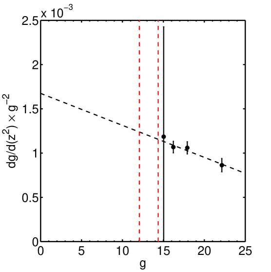
Figure 1: Data and linear fit for $g^{-2}dg/dz$.

We had to tune $\kappa$ to approach $z^{2}=10$. Table 1 shows that we were often successful within our small statistical errors. To implement the remaining tiny correction leading to the last column we have numerically determined the derivative $dg/d(z^{2})$. This is relatively easy by using the relation

$$t\frac{d}{dt}\langle\langle A\rangle\rangle=\langle\langle AK\rangle\rangle-\langle\langle A\rangle\rangle\langle\langle K\rangle\rangle$$ (16)

which holds in the loop representation [5]. In this formula $t\equiv\tanh(2\kappa)$ is used, $A$ can be any $\kappa$-independent observable and $K$ is the total number of links occupied by lines. We see in figure 1 that beyond $L=64$ the connected correlation (16) is too noisy to get a signal and we had to extrapolate with the shown linear fit. Its form is suggested by perturbation theory. We emphasize however that any error in this procedure only affects a systematic correction in the final results that itself is only of the order of the statistical error.

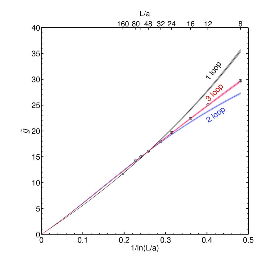
Figure 2: Cutoff dependence of the coupling $\tilde{g}$.

Our main result is now represented by figure 2. The curves show the evolution with the perturbative renormalization group at 1,2 and 3 loop precision where the evolution is started (in both directions) from our most precise data point at $L/a=48$. The shaded bands represent the small error of the initial value. We see a perfect match of all our data points with the three loop evolution and thus complete consistency with the (logarithmic) triviality scenario.

Acknowledgements: We thank Peter Weisz for discussions and the Deutsche Forschungsgemeinschaft (DFG) for support in the framework of SFB Transregio 9.

References

- [1] Johannes Siefert and Ulli Wolff, Triviality of theory in a finite volume scheme adapted to the broken phase, Phys. Lett. B 733 (2014) 11 [arXiv:1403.2570 [hep-lat]].
- [2] Ulli Wolff Triviality of four dimensional theory on the lattice, (2014) Scholarpedia, 9(10):7367.
- [3] M. Lüscher and P. Weisz, Scaling Laws and Triviality Bounds in the Lattice phi**4 Theory. 1. One Component Model in the Symmetric Phase, Nucl. Phys. B290 (1987) 25.
- [4] M. Lüscher and P. Weisz, Scaling Laws and Triviality Bounds in the Lattice phi**4 Theory. 2. One Component Model in the Phase with Spontaneous Symmetry Breaking, Nucl.Phys. B295 (1988) 65.
- [5] U. Wolff, Simulating the All-Order Strong Coupling Expansion I: Ising Model Demo, Nucl. Phys. B810 (2009) 491, [arXiv:0808.3934].
- [6] N. Prokof’ev and B. Svistunov, Worm Algorithms for Classical Statistical Models, Phys. Rev. Lett. 87 (2001) 160601, [arXiv:0910.1393].
- [7] P. Weisz and U. Wolff, Triviality of theory: small volume expansion and new data, Nucl. Phys. B846 (2011) 316–337, [arXiv:1012.0404].