Beyond the growth rate of cosmic structure:
Testing modified gravity models with an extra degree of freedom

Abstract

In ‘modified’ gravity the observed acceleration of the universe is explained by changing the gravitational force law or the number of degrees of freedom in the gravitational sector. Both possibilities can be tested by measurements of cosmological structure formation. In this paper we elaborate the details of such tests using the Galileon model as a case study. We pay attention to the possibility that each new degree of freedom may have stochastically independent initial conditions, generating different types of potential well in the early universe and breaking complete correlation between density and velocity power spectra. This ‘stochastic bias’ can confuse schemes to parametrize the predictions of modified gravity models, such as the use of the growth parameter $f$ alone. Using data from the WiggleZ Dark Energy Survey we show that it will be possible to obtain constraints using information about the cosmological-scale force law embedded in the multipole power spectra of redshift-space distortions. As an example, we obtain an upper limit on the strength of the conformal coupling to matter in the cubic Galileon model, giving $|1/M|\lesssim 200/M_{\mathrm{P}}$. This allows the fifth-force to be stronger than gravity, but is consistent with zero coupling.

I Introduction

The measurement of accelerated expansion is one of the most important discoveries in modern cosmology. But although this conclusion is now supported by multiple probes Betoule et al. (2014); Kazin et al. (2014); Anderson et al. (2014); Delubac et al. (2015); Hinshaw et al. (2013); Ade et al. (2014), we remain entirely ignorant of the underlying physics.

A microphysical explanation could arise from quantum fluctuations of the vacuum, which behave as a cosmological constant—a fluid with equation of state $p=-\rho$. But if this is the correct microphysical description it will be difficult to understand why the universe is accelerating so slowly. This has encouraged the growth of a large literature studying alternative explanations (for a review of such ideas, see Ref. Bull et al. (2016)).

If vacuum fluctuations are rejected, it seems inevitable that the acceleration must depend on new physics operating over very large scales which is not present in Einstein gravity. It is much less clear what this new physics should be, but at sufficiently low energies it is likely to appear to us in the form of extra scalar fields. These mediate long-range forces which compete with, or augment, the conventional $1/r^{2}$ gravitational force.

Any modification to the force law would influence the assembly of cosmic structures. Therefore, even if spatially-averaged properties—such as the time history of the expansion rate $H$—can be made to agree with a $\Lambda\text{CDM}$ model, the details of structure formation will often disagree. This makes measurements of structure formation a discriminating test of modified gravities. A sizeable industry has emerged which aims to detect departures from Einstein gravity by using surveys of the cosmological density and velocity fields to constrain the force law.

In modifications of gravity which entail extra fields there is another effect which is less frequently considered. According to current ideas, structure on all scales was seeded by quantum fluctuations which became imprinted on the gravitational potential $\Phi$ during an early inflationary epoch. The same effect will occur for every field which is light during inflation, generating a stochastically independent set of potential wells for each light degree of freedom in the gravitational sector. The implications of this scenario for the assembly of cosmic structure have not yet been worked out in detail.

Synopsis.—In this paper we study models of modified gravity with an extra scalar degree of freedom, and show that if inflation seeded a set of potential wells for this field they can renormalize the effective force law driving mass assembly. In addition, under certain circumstances they generate stochastic effects which could be visible in a sufficiently detailed galaxy survey. We show that constraints can be obtained from measurements of the ‘two-dimensional’ power spectrum $P(k,\mu)$, which incorporates information about both local densities and velocities as a function of redshift.

The paper is divided into three principal parts. In §II we generalize the analysis of density–density, density–velocity and velocity–velocity clustering statistics to models with extra forces and potential wells. We show that these statistics can be used to learn about the effective cosmological-scale force law and the number of dynamically relevant combinations of potentials.

In §III we describe a concrete model of this type, the cubic ‘Galileon’ scenario of Nicolis et al. Nicolis et al. (2009). We specialize the discussion of cosmological mass assembly from §II and address some of the issues which arise when deciding whether this model is a viable alternative to a simple cosmological constant.

In §IV we explain how the cubic Galileon model can be compared to a particular dataset constraining the velocity and density clustering statistics: the multipole power spectra measured by the WiggleZ Dark Energy Survey. We report the results in §V, and explain our conclusions in §VI.

We have tried to include sufficient explanation to make this paper relevant to both theorists and observers. Readers already familiar with measurements of the growth factor may wish to omit §II as far as §II.2. The earlier part is a review of standard material. In §III we have tried to summarize the motivation and relevance of ‘Galileon’ models of modified gravity, and to explain their current theoretical status. However, readers who are primarily interested in constraints on the model itself may prefer to skip most of §III on a first reading.

Notation.—Except when reporting observations, we work in natural units where $c=\hbar=1$. We express the strength of the gravitational force in terms of the reduced Planck mass, $M_{\mathrm{P}}=(8\pi G)^{-1/2}$, where $G$ is the conventional Newton constant. In our units, $M_{\mathrm{P}}$ has dimensions of energy with numerical value $M_{\mathrm{P}}=2.435\times 10^{18}\,\text{GeV}$. We measure the strength of fifth forces in energy units using a coupling scale $M$ which is analogous to $M_{\mathrm{P}}$.

II Structure formation and stochastic bias

In this section we review the analysis of structure formation in Einstein gravity (§II.1), assuming all perturbations to be seeded by a single primordial fluctuation, and show how it can be regarded as a test of the gravitational force law $\bm{\mathrm{{F}}}/m=-GM\hat{\bm{\mathrm{{r}}}}/r^{2}$. In §II.2 we generalize to the case of several independent primordial fluctuations.

Accretion onto overdensities.—In a statistically homogeneous and isotropic relativistic cosmological model we must describe gravity using two independent potentials $\Phi(\bm{\mathrm{{x}}},t)$ and $\Psi(\bm{\mathrm{{x}}},t)$. To first order in fluctuations, the metric is

$$\mathrm{d}s^{2}=-(1+2\Psi)\mathrm{d}t^{2}+a^{2}(1+2\Phi)\mathrm{d}\bm{\mathrm{{x}}}^{2}.$$ (1)

The scale factor $a$ is a function only of time $t$. In Einstein gravity, at this order, the potentials are equal up to a sign in the absence of anisotropic stress. We are assuming that the prehistory of the observable universe has selected the flat Friedmann–Robertson–Walker metric, perhaps as a result of an inflationary era.

At early times the universe consists of matter and radiation. The background densities are $\rho_{m}$, $\rho_{r}$ and we assume small perturbations $\delta\rho_{m}\equiv\delta_{m}\rho_{m}$, $\delta\rho_{r}\equiv\delta_{r}\rho_{r}$. The spatial configuration of each fluid is rearranged by flow fields or ‘velocity perturbations’ $\bm{\mathrm{{v}}}_{m}$, $\bm{\mathrm{{v}}}_{r}$. In the potential flow approximation we can represent these perturbations by the divergence $\theta=\bm{\mathrm{{\nabla}}}\cdot\bm{\mathrm{{v}}}$.

In a Newtonian model we would obtain a dynamical equation by balancing the sum of forces $\sum_{i}\bm{\mathrm{{F}}}_{i}$ on a small element of fluid. Expressing this balance equation in terms of $\theta$, allowing for an expanding universe and the possibility of a modified gravitational force law, we find

$$\frac{\mathrm{d}\theta_{m}}{\mathrm{d}t} =-2H\theta_{m}-\frac{\partial^{2}}{a^{2}}\Psi+F_{5m}$$ (2a)

$$\frac{\mathrm{d}\theta_{r}}{\mathrm{d}t} =-H\theta_{r}-\frac{\partial^{2}}{a^{2}}\Psi-\frac{1}{4}\frac{\partial^{2}}{a^{2}}\delta_{r}+F_{5r}.$$ (2b)

Here, $-\partial\Psi$ is the static gravitational force, terms proportional to $H\theta$ represent Hubble friction, and $F_{5m}$, $F_{5r}$ describe (the divergence of) possible fifth-forces acting on matter and radiation, respectively. They are zero in pure Einstein gravity. The term proportional to $\delta_{r}$ in Eq. (2b) represents an additional force due to the internal pressure of radiation.

Eqs. (2a)–(2b) are dynamical. They show that linear growth of cosmological structure is essentially an infall experiment accounting for work done against the expansion $H$. To close this system requires further kinematic equations describing the deposition of excess radiation or matter into each fluid element. These are

$$\frac{\mathrm{d}\delta_{m}}{\mathrm{d}t} =-\theta_{m}-3\dot{\Phi}+j_{5m}$$ (3a)

$$\frac{\mathrm{d}\delta_{r}}{\mathrm{d}t} =-\frac{4}{3}\theta_{r}-4\dot{\Phi}+j_{5r},$$ (3b)

where $j_{5m}$, $j_{5r}$ represent matter and radiation fluxes induced by fifth-forces. The mass-energy deposited by the flows $\bm{\mathrm{{v}}}_{m}$, $\bm{\mathrm{{v}}}_{r}$ is described by the terms proportional to $\theta_{m}$, $\theta_{r}$, whereas the terms proportional to $\dot{\Phi}$ describe changes in density due to relativistic modulation of the proper volume by $\Phi$. This approach, where deviations from the predictions of Einstein gravity are modelled as fifth forces and fluxes, was employed in Ref. Burrage et al. (2016).

II.1 Einstein gravity

In Einstein gravity there are no fifth forces or fluxes, and on subhorizon scales the modulation due to $\dot{\Phi}$ is negligible and can be discarded. This is the ‘quasi-static’ approximation. In this limit changes in density are entirely due to deposition by the flow, and the deposition equation for matter can be rewritten as a definition of the growth factor $f$,

$$\frac{\mathrm{d}\ln\delta_{m}}{\mathrm{d}\ln a}\equiv f=-\frac{\theta_{m}}{H\delta_{m}}.$$ (4)

When reporting the results of velocity surveys it is conventional to measure $\theta$ in Hubble units, corresponding to the rescaling $\theta\mapsto\theta/H$. In what follows we normalize $\theta$ in this way, after which (4) becomes $\theta_{m}=-f\delta_{m}$.

In this model the growth rate is spatially independent, and therefore (4) implies that $\theta_{m}$ is totally correlated with $\delta_{m}$ up to a bias $-f$ depending on the rate of deposition. According to Eq. (2a) this deposition is maintained purely by gravitational forces. As we describe in Eq. (7) and below, this makes the precise value of $f$ depend on details of the gravitational force law.

In Einstein gravity the force law is determined by the Poisson constraint

$${-\frac{k^{2}}{a^{2}}}\Psi=\frac{\rho}{2M_{\mathrm{P}}^{2}}\left(\delta_{m}+3H\frac{a^{2}}{k^{2}}\theta_{m}\right)$$ (5)

together with the ‘no-slip’ condition $\Phi=-\Psi$. The strength of the force is measured by the Planck mass $M_{\mathrm{P}}=(8\pi G)^{-1/2}$. On subhorizon scales the Poisson constraint expresses the familiar inverse-square law $\bm{\mathrm{{F}}}/m=-GM\hat{\bm{\mathrm{{r}}}}/r^{2}$. In modified gravity, changes to the $1/r^{2}$ force law are sometimes expressed as a scale- or redshift-dependent $G$ or Planck mass $M_{\mathrm{P}}$, viz. $M_{\mathrm{P}}^{2}(k)\equiv\beta(k)(M_{\mathrm{P}}^{2})_{0}$ where $\beta(k)\rightarrow 1$ as $k\rightarrow 0$ and $(M_{\mathrm{P}}^{2})_{0}$ represents the strength of gravity on very large scales. Then $\beta(k)$ represents a correction to the $1/r^{2}$ law on smaller scales.

This parametrization of a scale-dependent force law is conventional in the modified-gravity community. Note that $\beta(k)$ defined in this way is unconnected with the ratio of $f$ to the bias, $f/b$, also denoted $\beta$ within the large-scale structure community.

Example: change to $1/r^{2}$ law.—Combining Eqs. (2a), (3a) and (5) yields the Mészáros equation. Allowing for scale-dependent modifications to the force law but assuming the Friedmann equation is sensitive only to the long-wavelength force, the Mészáros equation can be written (assuming an $\Omega_{m}=1$ cosmology)

$$\ddot{\delta}_{m}+\frac{4}{3t}\dot{\delta}_{m}-\frac{2\beta(k)^{-1}}{3t^{2}}\delta_{m}=0.$$ (6)

The corresponding scale-dependent growth rate is

$$f(k)=\frac{-1+\sqrt{1+24\beta(k)^{-1}}}{4}.$$ (7)

If $\beta$ decreases then the effective gravitational force increases, as does $f$. If $\beta$ increases, the reverse is true.

Given measurements of $f(k)$ it is possible to recover $\beta(k)$, from which the behaviour of the force law could be extracted via a Fourier transform. The outcome is that combined probes of the velocity and density perturbations serve a similar purpose to laboratory tests of the inverse-square law, but on vastly different scales.

In this $\Omega_{m}=1$ model, if $f=1$ the force law is precisely proportional to $1/r^{2}$. Deviations from $f=1$ signal deviations from inverse-square-law behaviour. Current data favour $f\sim 0.5$, which can be interpreted as a softening on cosmological scales due to the repulsion of dark energy counteracting the attraction of Newtonian gravity. A more detailed discussion of the effect of dark energy perturbations was given by Nesseris & Sapone Nesseris and Sapone (2015).

II.2 Modified gravities

In more complex models the interpretation of $f$ becomes less clear, because we must separate the effects of scale- and time-dependence in the force law from work done against the expansion. We do not know in advance what should be attributed to any of these sources. Nevertheless, provided only a single set of primordial potential wells exist, $f$ can be regarded as a measure of the effective gravitational force including cosmological effects. Under these circumstances it is a deterministic function, independent of position, making $\delta_{m}$ and $\theta_{m}$ completely correlated as above.

In models with fifth-forces it is possible for inflation to seed more than one stochastically independent set of potential wells. As we explain below, the local growth rate can be influenced by contributions from each set and we must regard $f$ as a probe not only of the force law but also of the initial conditions. In this section our aim is to set up a framework which is sufficiently general to describe models of this kind.

Single set of potential wells.—If $f$ is not a fixed number but varies from place to place, we speak of stochastic bias. Where stochastic effects are important, the predictions of a physical model become statistical statements about the expected value or distribution of observables. Therefore the discussion should be framed in terms of correlation functions rather than quantities such as $\delta$, $\theta$ or $\Phi$ which are not directly measurable.

First, we replicate the discussion of Einstein gravity in this language, assuming there is only a single primordial fluctuation which is responsible for sourcing the large-scale matter distribution and its flow, normally ascribed to the Newtonian potential $\Phi$. We suppose it has attained a practically time-independent value $\Phi^{\ast}(\bm{\mathrm{{x}}})$ by some time early in the radiation era. Then, at some later time $t$, the matter and flow fields can be written

$$\delta_{m}(k,t) ={T_{{\delta}}}^{{\Phi}}(k,t)\Phi^{\ast}(k)$$ (8a)

$$\theta_{m}(k,t) ={T_{{\theta}}}^{{\Phi}}(k,t)\Phi^{\ast}(k),$$ (8b)

where we have assumed statistical isotropy and ${T_{{i}}}^{{j}}$ is a transfer function describing how an initial fluctuation in field $j$ is reprocessed into a later configuration of field $i$. In this subsection $\delta$ and $\theta$ always refer to the matter density and velocity, and we drop the distinguishing subscript ‘$m$’.

In analogy with the definition $-f=\theta/\delta$ we define an effective (but possibly scale- and time-dependent) bias by

$$f_{\text{eff}}(k)\equiv-\frac{{T_{{\theta}}}^{{\Phi}}(k)}{{T_{{\delta}}}^{{\Phi}}(k)}=-\frac{\theta(k)}{\delta(k)},$$ (9)

in which the stochastic initial condition has been ‘divided out’. In this equation and what follows we suppress the dependence of $f_{\text{eff}}$ and ${T_{{i}}}^{{j}}$ on time.

Still assuming only a single primordial perturbation, $f_{\text{eff}}(k)$ could equivalently be defined using the relative normalization of the different two-point correlation functions,

$$\langle\delta\theta\rangle_{k} =-f_{\text{eff}}(k)\langle\delta\delta\rangle_{k}$$ (10a)

$$\langle\theta\theta\rangle_{k} =f_{\text{eff}}(k)^{2}\langle\delta\delta\rangle_{k},$$ (10b)

Eqs. (10a)–(10b) deal with stochasticity by averaging over it, rather than dividing it out as in (9).

Eqs. (10a)–(10b) characterize ‘deterministic’ bias, which is associated with a fixed multiplicative normalization between $\langle\delta\delta\rangle$, $\langle\delta\theta\rangle$ and $\langle\theta\theta\rangle$. This fixed change in normalization is the signature of complete correlation between $\theta$ and $\delta$. Attempts have been made to detect this bias experimentally Blake et al. (2011).

Multiple sets of potential wells.—We now add a fifth force, mediated by a scalar field $\phi$ which we also assume to have received a primordial inflationary fluctuation $\delta\phi^{\ast}(k)$. We suppose that $\delta\phi^{\ast}(k)$ achieves a time-independent value by the onset of radiation domination in the same way as the gravitational potential. If $\phi$ is active during inflation this could leave $\Phi^{\ast}$ and $\delta\phi^{\ast}$ partially or entirely correlated. However, simple models can produce the uncorrelated case $\langle\Phi\delta\phi\rangle^{\ast}=0$ and in this paper we focus on scenarios of that type.

Even if the primordial fluctuations $\Phi^{\ast}$ and $\delta\phi^{\ast}$ are uncorrelated they will mix in the late-time matter and flow fields. Physically this corresponds to a competition between gravity and the new fifth force to attract matter into their respective potential wells. Therefore we must now write

$$\delta(k) ={T_{{\delta}}}^{{\Phi}}(k)\Phi^{\ast}(k)+{T_{{\delta}}}^{{\phi}}(k)\delta\phi^{\ast}(k)$$ (11a)

$$\theta(k) ={T_{{\theta}}}^{{\Phi}}(k)\Phi^{\ast}(k)+{T_{{\theta}}}^{{\phi}}(k)\delta\phi^{\ast}(k).$$ (11b)

We define growth factors associated with $\Phi$ and $\delta\phi$,

$$f_{\text{eff}}^{\Phi} =-\frac{{T_{\theta}}^{\Phi}}{{T_{\delta}}^{\Phi}}$$ (12a)

$$f_{\text{eff}}^{\phi} =-\frac{{T_{\theta}}^{\phi}}{{T_{\delta}}^{\phi}}.$$ (12b)

These characterize the strength and scale dependence of the force law associated with infall into each type of potential well. The relationship between the $\langle\delta\delta\rangle$, $\langle\theta\delta\rangle$ and $\langle\theta\theta\rangle$ correlation functions becomes

$$\langle\theta\delta\rangle_{k} =\langle\delta\delta\rangle_{k}\bigg{(}{-f_{\text{eff}}^{\Phi}(k)}+\frac{f_{\text{eff}}^{\Phi}(k)-f_{\text{eff}}^{\phi}(k)}{1+\rho(k)}\bigg{)}$$ (13a)

$$\langle\theta\theta\rangle_{k} =\langle\theta\delta\rangle_{k}\bigg{(}{-f_{\text{eff}}^{\Phi}(k)}+\frac{f_{\text{eff}}^{\Phi}(k)-f_{\text{eff}}^{\phi}(k)}{1+\sigma(k)}\bigg{)}$$ (13b)

$$=\langle\delta\delta\rangle_{k}\bigg{(}f_{\text{eff}}^{\Phi}(k)^{2}+\frac{f_{\text{eff}}^{\phi}(k)^{2}-f_{\text{eff}}^{\Phi}(k)^{2}}{1+\rho(k)}\bigg{)}.$$ (13c)

These equations assume the primordial decorrelation condition $\langle\Phi\delta\phi\rangle^{\ast}=0$ and would require modification were it to be abandoned.

The clustering power is given by summing the contribution from each set of potential wells. The same is true for the velocity power. In Eqs. (13a)–(13c) we have introduced parameters $\rho$ and $\sigma$ which measure the relative contributions to the $\delta\delta$ and $\theta\delta$ correlation functions from each set of potentials. They satisfy

$$\rho(k) \equiv\frac{({T_{\delta}}^{\Phi})^{2}}{({T_{\delta}}^{\phi})^{2}}\frac{\langle\Phi\Phi\rangle^{\ast}}{\langle\delta\phi\delta\phi\rangle^{\ast}}$$ (14a)

$$\sigma(k) \equiv\frac{{T_{\theta}}^{\Phi}{T_{\delta}}^{\Phi}}{{T_{\theta}}^{\phi}{T_{\delta}}^{\phi}}\frac{\langle\Phi\Phi\rangle^{\ast}}{\langle\delta\phi\delta\phi\rangle^{\ast}}$$ (14b)

If the clustering power is dominated by accumulation within the $\Phi^{\ast}$ potential wells then $\rho\gg 1$, whereas if it is dominated by accumulation within the $\delta\phi^{\ast}$ potential wells then $\rho\ll 1$. A similar statement holds for $\sigma$.

Eqs. (13a)–(13c) show that, depending which set of potential wells dominate the correlation functions, their relative normalization interpolates between $f_{\text{eff}}^{\Phi}$ and $f_{\text{eff}}^{\phi}$. Where only Newtonian potential wells are relevant the effective growth factor is $f_{\text{eff}}^{\Phi}$, and where only Galileon potential wells are relevant the effective growth factor is $f_{\text{eff}}^{\phi}$.

In a typical model there are two possibilities. First, matter may accumulate within just one of the primordial potentials, perhaps $\Phi^{\ast}$. Taking this as an example, the fifth force will still be relevant if it modifies the background expansion history or its perturbations couple to $\Phi$. Either possibility can introduce scale- or time-dependent modifications of the Newtonian force law, leading to changes in $f_{\text{eff}}^{\Phi}$—but the growth factors measured from different combinations of the two-point functions will agree. The net effect is a Galileon analogue of the ‘softening’ from $f=1$ to $f\sim 0.5$ due to dark energy in a $\Lambda\text{CDM}$ model. This scenario was studied by Appleby & Linder in the case where the fifth-force field $\phi$ has Galileon interactions. They found it to be incompatible with observation if the Galileon made a significant contribution to the expansion history Appleby and Linder (2012, 2012).

Alternatively, matter may accumulate in a combination of the $\Phi^{\ast}$ and $\delta\phi^{\ast}$ potential wells. The net force driving inflow into this combination will be an admixture of the force laws associated with each type of potential well. As we explain below, in the most favourable circumstances we may be able to observe different combinations of these laws using different combinations of the two-point functions such as $-\langle\theta\delta\rangle/\langle\delta\delta\rangle$ and $-\langle\theta\theta\rangle/\langle\theta\delta\rangle$. In this scenario we could measure at least two different effective growth factors. Further combinations become available where more than one fifth-force field and corresponding set of potential wells exist. A qualitatively similiar discussion applies if $\Phi^{\ast}$ and $\delta\phi^{\ast}$ are correlated, although modified in detail because the force laws no longer operate independently.

This ‘decorrelation’ occurs only if $\sigma(k)$ is appreciably different to $\rho(k)$, so that the power in $\langle\delta\delta\rangle$ and $\langle\theta\delta\rangle$ is dominated by clustering around different combinations of the potential wells. For example, this might happen if most matter has accumulated in one combination of potentials but a strong flow is driving exchange with the orthogonal combination. Such decorrelations are the signature of nondeterministic or stochastic bias. If it occurs the signature is unambiguous because the relationship between the two-point functions cannot be mimicked by any choice of deterministic bias, even one which is scale-dependent. The deterministic model implies that different ways to measure the growth factor must agree, because they are always measuring the same force law. Specifically,

$$\frac{\langle\theta\theta\rangle}{\langle\theta\delta\rangle}-\frac{\langle\theta\delta\rangle}{\langle\delta\delta\rangle}=\Big{(}f_{\text{eff}}^{\Phi}-f_{\text{eff}}^{\phi}\Big{)}\frac{\rho-\sigma}{(1+\rho)(1+\sigma)},$$ (15)

and the right-hand side is zero in a deterministic model irrespective of the force law and the primordial power spectrum. Whether departures from zero are measurable depends on $\rho$, $\sigma$ and the split between $f_{\text{eff}}^{\Phi}$ and $f_{\text{eff}}^{\phi}$. In §§IV–V we will study this sort of decorrelation in a concrete Galileon model.

A systematic study of the relative magnitude of $\langle\delta\delta\rangle$, $\langle\delta\theta\rangle$ and $\langle\theta\theta\rangle$ as functions of scale therefore yields two outcomes. First, we probe the effective strength and scale-dependence of the gravitational force law. Second, we determine whether a single combination of potential wells was relevant during structure formation, or whether there is evidence for a more complex model.

Similar effects can occur for any pair of fluctuations. For example, in certain models of modified gravity, the first-order relation $\Phi=-\Psi$ is violated (described as ‘slip’). This can be probed through combinations of observables that measure both metric potentials, such as weak gravitational lensing or the integrated Sachs–Wolfe effect. Stochastic effects would generate systematic shifts between the correlation functions of $\delta$ with (for example) the weak-lensing shear $\gamma$, or the ISW temperature decrement, that are not simply fixed changes in normalization. The effectiveness of such combinations for constraints on non-minimally coupled modified-gravity models was studied by Gleyzes et al., although the analysis is limited to the quasi-static approximation Gleyzes et al. (2016).

Valkenburg & Hu have made available a code for generating initial conditions for cosmological N-body simulations, which accommodates perturbation spectra that are decorrelated or anticorrelated between the matter and extra scalar degree of freedom Valkenburg and Hu (2015).

III Galileon modified gravity

In the remainder of this paper we apply the formalism developed in §II to a specific model for the fifth-force field $\phi$, which we take to be a Galileon Nicolis et al. (2009). We do not make use of the quasi-static approximation. In §III.1 we briefly recall the relevance of the model for scenarios of modified gravity, and in §III.2 we discuss the background cosmological solution and its expansion history. In §III.3 we prepare for the calculation of effective growth factors by specializing the structure-formation equations from §II. Finally, in §III.4 we discuss the criteria which should be used to decide whether the model suffers from objections similar to those which led us to reject a simple cosmological constant.

III.1 The Galileon model

A Galileon is a normal scalar field whose self-interactions are restricted to be of a special kind Deffayet et al. (2009, 2009). The action for a Galileon coupled to gravity is of the form

$$S=\int\mathrm{d}^{4}x\;\sqrt{-g}\Big{(}\frac{M_{\mathrm{P}}^{2}}{2}R-\frac{1}{2}\sum_{2\leqslant i\leqslant 5}c_{i}\Lambda^{3(2-i)}\mathcal{L}_{i},\Big{)}$$ (16)

where $g_{ab}$ is the metric, $R$ is the Ricci scalar built from $g_{ab}$ and its Levi–Civita connexion, and the allowed $\mathcal{L}_{i}$ are

$$\mathcal{L}_{2} =(\nabla\phi)^{2}$$ (17a)

$$\mathcal{L}_{3} =(\nabla\phi)^{2}\Box\phi$$ (17b)

$$\mathcal{L}_{4} =(\nabla\phi)^{2}\Big{[}2(\Box\phi)^{2}-2\phi_{;\mu\nu}\phi^{;\mu\nu}-\frac{R}{2}(\nabla\phi)^{2}\Big{]}$$ (17c)

$$\mathcal{L}_{5} =(\nabla\phi)^{2}\Big{[}(\Box\phi)^{3}-3(\Box\phi)\phi_{;\mu\nu}\phi^{;\mu\nu}$$

$$\qquad\qquad\hskip 5.69054pt\mbox{}+2{\phi_{;\mu}}^{\nu}{\phi_{;\nu}}^{\rho}{\phi_{;\rho}}^{\mu}-6G_{\nu\rho}\phi_{;\mu}\phi^{;\mu\nu}\phi^{;\rho}\Big{]}.$$ (17d)

A semicolon denotes the covariant derivative compatible with $g_{ab}$ and $G_{\nu\rho}$ is the Einstein tensor. We have also used $(\nabla\phi)^{2}=g^{ab}\phi_{;a}\phi_{;b}$ and $\Box\phi=g^{ab}\phi_{;ab}$. If there are no hierarchies in the Galileon sector it will be possible to choose $\Lambda$ so that the $c_{i}$ are of order unity. Then $\Lambda$ determines where the higher-order interactions $\mathcal{L}_{3}$, $\mathcal{L}_{4}$ and $\mathcal{L}_{5}$ become comparable to $\mathcal{L}_{2}$.

The Galileon model is an interesting example in which to test probes of modified gravity. We adopt it for several reasons:

1. Screening through the Vainshtein mechanism.—Although $\phi$ mediates a fifth force, it may be dynamically suppressed (‘screened’) sufficiently close to heavy objects due to nonlinear effects associated with the scale $\Lambda$ Nicolis et al. (2009); Burrage and Seery (2010). Dealing correctly with such nonlinear screening effects is expected to be important for realistic scenarios.

Several distinct screening mechanisms exist Joyce et al. (2015). Galileons exhibit a type known as ‘Vainshtein’ screening, in which suppression of the fifth force occurs rather softly and over large distances. The WiggleZ survey, which we will use for comparison to data, is particuarly suitable for tests of Vainshtein-type screening because most objects in the survey are field galaxies far from cluster centres. This offers an opportunity to probe the transition from screened to unscreened fifth forces around cluster outskirts.

In addition to screening of sources, there can be ‘cosmological’ screening which universally suppresses fifth forces when the mean cosmological energy density is large. The Galileon model exhibits this ‘cosmological’ Vainshtein effect Chow and Khoury (2009).

2. Versatile interpretation.—Galileon models contain no physics which could solve the cosmological constant problem, but it is possible that they approximate the long-wavelength behaviour of other (currently unknown) physics which does. In particular:

1. If the effective cosmological constant is somehow set to zero, late-time acceleration could be supported by an energy density associated with $\phi$. As explained in §II, this possibility has been considered by Appleby & Linder and later authors Appleby and Linder (2012, 2012); Barreira et al. (2012); Okada et al. (2013); Barreira et al. (2013, 2013), who found that it led to changes in the growth of cosmic structure which were excluded by observation. Other constraints on Galileon models which do not explicitly couple to matter have been obtained by Barreira et al. using observations of the cosmic microwave background and baryon acoustic oscillations Barreira et al. (2014).

2. Alternatively, $\phi$ may have no role in supporting late-time acceleration but merely be a vestige of whatever physics is responsible for it. For example, this might happen in a massive gravity where the graviton mass is responsible for ‘degravitating’ the cosmological constant. Then $\phi$ is an unavoidable by-product of the graviton mass but is not otherwise important. Galileon models have been shown to arise in this way from the de Rham–Gabadadze–Tolley massive gravity de Rham and Gabadadze (2010); de Rham et al. (2011). In this scenario $\phi$ has negligible energy density.

For the second possibility there are two relevant questions: first, whether expansion histories exist in which the Galileon is always subdominant; and second, whether its contribution to the effective gravitational force nevertheless excludes the model. In this paper we focus on scenarios of this type.

3. Sufficiently concrete.—The model is sufficiently well-defined that we can (and should) apply an analysis similar to the logic which led us to reject vacuum fluctuations as an explanation for the microphysics of acceleration. This is important because nothing is gained by replacing a simple model with a more complex one which suffers from the same drawbacks. We discuss this issue in §III.4.

III.2 Cosmological background expansion

We focus on the cubic Galileon model, for which only $c_{2}$ and $c_{3}$ are nonzero. This is numerically simplest and already includes the interesting features of the $\mathcal{L}_{4}$ and $\mathcal{L}_{5}$ terms, except for anisotropic stress which (to first-order in perturbations) is identically zero for $\mathcal{L}_{3}$.

Matter species.—We take the matter to consist of radiation and pressureless dust representing cold dark matter, which we couple to $\phi$ via the conformal transformation

$$g_{\mu\nu}\mapsto\Big{(}1+\frac{\phi}{M}\Big{)}g_{\mu\nu}$$ (18)

within the matter Lagrangian. This means that $\phi$ couples to the trace of the energy–momentum tensor $T={T^{a}}_{a}$ for the matter fields via an interaction of the form $\phi T/M$. For a mix of matter and radiation the trace $T$ equals the matter density $\rho_{m}$.

When measured using the Einstein-frame metric $g_{\mu\nu}$ this conformal coupling makes the matter density and pressure $\phi$-dependent. They are related to their $\phi$-independent Jordan-frame counterparts $\rho^{J}$, $p^{J}$ (which can be regarded as the ‘intrinsic’ density and pressure for the fluid) by the rule

$$\rho =\Big{(}1+\frac{\phi}{M}\Big{)}\rho^{J}$$ (19a)

$$p =\Big{(}1+\frac{\phi}{M}\Big{)}p^{J}.$$ (19b)

The $\phi$-dependence allows the Einstein-frame fluid to exchange energy with the Galileon, described by the continuity equations

$$\frac{\mathrm{d}\rho_{m}}{\mathrm{d}t}+3H\rho_{m} =-\frac{1}{2M}\frac{\mathrm{d}\phi}{\mathrm{d}t}\Big{(}1+\frac{\phi}{M}\Big{)}^{-1}\rho_{m}$$ (20a)

$$\frac{\mathrm{d}\rho_{r}}{\mathrm{d}t}+4H\rho_{r} =0,$$ (20b)

where $t$ is the Einstein-frame time, $H$ is the corresponding Hubble parameter, and $\rho_{m}$ and $\rho_{r}$ are, respectively, the energy density in CDM and radiation. Eq. (20b) shows that the radiation is conserved separately, without exchanging energy with any other component. This happens because the action for radiation is classically conformally invariant.

Galileon evolution.—The Galileon field profile is controlled by the field equation

$$c_{2}\Box\phi+\frac{c_{3}}{\Lambda^{3}}[(\Box\phi)^{2}-\partial_{\mu}\partial_{\nu}\phi\partial^{\mu}\partial^{\nu}\phi]-\frac{1}{2M}\Big{(}1+\frac{\phi}{M}\Big{)}^{-1}T=0,$$ (21)

If they are required, expressions for the contribution of each higher-order Galileon operator to the equation of motion can be found in Refs. Nicolis et al. (2009); Deffayet et al. (2009). We include all nonlinear effects in $\phi$ because these are important to correctly capture the ‘cosmological’ Vainshtein effect, described in more detail below.

Specialising to the background cosmological evolution, Eq. (21) can be expressed as a continuity equation for $\phi$,

$$\frac{\mathrm{d}\rho_{\phi}}{\mathrm{d}t}+3H(\rho_{\phi}+p_{\phi})=\frac{\dot{\phi}}{2M}\Big{(}1+\frac{\phi}{M}\Big{)}^{-1}\rho_{m}.$$ (22)

It can be checked that (20a), (20b) and (22) together imply total conservation of energy.

Cosmological Vainshtein effect.—We are focusing on scenarios where the Galileon remains a subdominant contributor to the universe’s expansion history. To achieve this we must select a suitable trajectory for the background $\phi$ field, which we describe as the ‘cosmological Vainshtein solution’. We seek a solution in which nonlinear effects dominate the field profile. The background Galileon configuration evolves according to

$$c_{2}(\ddot{\phi}+3H\dot{\phi})+\frac{c_{3}}{\Lambda^{3}}\Big{[}\frac{\mathrm{d}}{\mathrm{d}t}(H\dot{\phi}^{2})+3H^{2}\dot{\phi}^{2}\Big{]}=-\frac{\rho_{m}}{2M}.$$ (23)

Assuming the $c_{3}$ term is dominant and that $H\sim 1/t$, which is the case during matter and radiation domination, then

$$\dot{\phi}\sim\frac{\Lambda}{H}\sqrt{-\frac{\rho_{m}\Lambda}{c_{3}M}}.$$ (24)

We must choose $\Lambda>0$ to give $\phi$ a stable kinetic term, so this ‘cosmological Vainshtein solution’ exists only if $M<0$. The same conclusion was reached by Chow & Khoury, who studied cosmological evolution in a number of Galileon models Chow and Khoury (2009). Note that the sign of $M$ has no effect on the nature of the force mediated between matter particles by $\phi$. This depends on $M^{2}$ and is always attractive.

On the solution (24) the Galileon energy density relative to matter can be written

$$\frac{\rho_{\phi}}{\rho_{m}}=-\frac{1}{c_{3}^{1/3}}\frac{M_{\mathrm{P}}}{\Lambda}\left(\frac{3\Lambda}{2|M|}\right)^{3/2}\left(\frac{\rho_{m}}{\rho_{m}+\rho_{r}}\right)^{1/2}.$$ (25)

Therefore $\rho_{\phi}$ is negative, leading to catastrophic consequences if the Galileon energy density becomes a significant fraction of the total energy budget. This is a pathology peculiar to the cubic Galileon model.

We intend (25) to apply for a strongly self-interacting model where $\Lambda\ll|M|\lesssim M_{\mathrm{P}}$. With these choices it is possible for the Galileon energy density to remain small compared to the matter energy density for much of the lifetime of the universe, and the problem can be avoided. The precise Galileon contribution is controlled by the relative abundance of matter and radiation.

The cosmological Vainshtein solution is an attractor in the space of solutions Appleby and Linder (2012); De Felice and Tsujikawa (2012). It is valid provided

$$\frac{c_{2}^{2}}{c_{3}}\Lambda^{3}|M|\lesssim\rho_{m}.$$ (26)

The left-hand side is fixed once we have chosen values for $c_{2}$, $c_{3}$, $\Lambda$ and $M$. These should be selected so that (26) is satisfied at early times. However, as the matter density dilutes (26) must eventually be invalidated, causing the Galileon to contribute an increasing fraction of the total energy budget. In the cubic model this leads to a singularity because of (25). If we demand that (26) is valid until today, in order to obtain a nearly $\Lambda\text{CDM}$-like expansion history down to redshift $z\sim 0$, we obtain a rough constraint $\Lambda\lesssim 10^{-13}(M_{\mathrm{P}}/|M|)^{1/3}\,\text{eV}$.

As a side effect, the cosmological Vainshtein solution suppresses Galileon fifth forces while the average cosmological energy density is sufficiently large. This will be discussed further in §IV.2.

III.3 Perturbations and structure formation

Perturbations in the Galileon model can be described using the general formalism assembled in §II.

Governing equations.—The dynamical and deposition equations are (2a)–(2b) and (3a)–(3b), with the fifth forces and fluxes

$$F_{5m} =\frac{1}{2M}\Big{(}1+\frac{\phi}{M}\Big{)}^{-1}\Big{(}\dot{\phi}\theta_{m}+\frac{\partial^{2}}{a^{2}}\delta\phi\Big{)}$$ (27a)

$$j_{5m} =-\frac{\delta\dot{\phi}}{2M}\Big{(}1+\frac{\phi}{M}\Big{)}^{-1}+\frac{\dot{\phi}}{2M}\frac{\delta\phi}{M}\Big{(}1+\frac{\phi}{M}\Big{)}^{-2}$$ (27b)

$$F_{5r} =j_{5r}=0.$$ (27c)

The fifth-force divergence $F_{5m}$ which sources the matter flow consists of a potential-gradient contribution proportional to $\partial^{2}\phi$ and a reaction term proportional to $\dot{\phi}\theta_{m}$. The reaction term arises from changes in momentum due to conversion of matter into $\phi$. The flux $j_{5m}$ represents the effective deposition of matter due to the reverse process, in which energy density from $\phi$ is locally converted into matter. The radiation is not coupled to $\phi$ and is therefore unaffected, giving $F_{5r}=j_{5r}=0$.

We also require an evolution equation for the Galileon perturbation $\delta\phi$, which can be written

$$D_{2}\delta\ddot{\phi}+\cdots=\frac{\rho_{m}\delta_{m}}{2M}\Big{(}1+\frac{\phi}{M}\Big{)}^{-1}-\frac{\rho_{m}}{2M}\frac{\delta\phi}{M}\Big{(}1+\frac{\phi}{M}\Big{)}^{-2},$$ (28)

where $D_{2}=-c_{2}+6c_{3}H\dot{\phi}/\Lambda^{3}$ is a coefficient depending on the background cosmology and Galileon evolution, and ‘$\cdots$’ denotes a series of terms that are first-order in perturbations, all of which enter with coefficients that are functions of the background quantities. Full expressions for all these coefficients are given by de Felice, Kase & Tsujikawa De Felice et al. (2011).

Initial conditions.—We set initial conditions in the radiation era. The Galileon field velocity is chosen to select the cosmological Vainshtein solution (24).

The density and velocity perturbations inherit their initial amplitudes from the primordial Newtonian and Galileon potentials. In the cubic Galileon model there is no anisotropic stress to first order, and therefore at this order the Einstein equations require $\Phi=-\Psi$. We work in terms of $\Phi$. On superhorizon scales, deep in the radiation era where both matter and Galileon densities are negligible, the initial condition is

$$\delta_{r}^{\ast}(\bm{\mathrm{{k}}})=2\Phi^{\ast}(\bm{\mathrm{{k}}}),$$ (29)

where a superscript ‘$\ast$’ denotes evaluation at the initial time.

As explained in §II, we are taking $\Phi^{\ast}$ and $\delta\phi^{\ast}$ to be stochastic random fields whose statistical properties are determined by a prior inflationary phase, and we are assuming that $\langle\Phi\delta\phi\rangle^{\ast}=0$. We take the $\Phi^{\ast}$ two-point function to satisfy

$$\langle\Phi(\bm{\mathrm{{k}}}_{1})\Phi(\bm{\mathrm{{k}}}_{2})\rangle^{\ast}=(2\pi)^{3}\delta(\bm{\mathrm{{k}}}_{1}+\bm{\mathrm{{k}}}_{2})\frac{A_{\Phi}}{k^{3}}\Big{(}\frac{k}{k_{0}}\Big{)}^{n_{s}-1},$$ (30)

where $A_{\Phi}$ is an amplitude to be fixed using Planck measurements of the microwave background power spectrum, and $n_{s}$ is a spectral index. We also assume that during inflation $\delta\phi$ was light enough to receive a quantum fluctuation and write its two-point function

$$\langle\delta\phi(\bm{\mathrm{{k}}}_{1})\delta\phi(\bm{\mathrm{{k}}}_{2})\rangle^{\ast}=(2\pi)^{3}\delta(\bm{\mathrm{{k}}}_{1}+\bm{\mathrm{{k}}}_{2})\frac{A_{\phi}}{k^{3}}.$$ (31)

We define the amplitude $A_{\phi}$, and likewise $A_{\Phi}$ and $n_{s}$, at the Planck pivot scale $k_{0}=0.05\,\text{Mpc}^{-1}$. In this paper we assume the $\delta\phi$ fluctuations do not have a significant scale dependence. We use the Planck2013+WP best-fit value $n_{s}=0.9619$ and assume no running Ade et al. (2014).

To fix the amplitudes $A_{\Phi}$ and $A_{\phi}$ we use the Planck2013+WP best-fit value for the amplitude of the primordial curvature perturbation power spectrum, $A_{s}=2.215\times 10^{-9}$, to infer the $\Phi$ power spectrum on a large scale $k=0.001h/\text{Mpc}$ measured by Planck near $z\sim 1000$ in their best-fit $\Lambda\text{CDM}$ cosmology. We assume a fixed ratio $\xi$ between the depths of the primordial Newtonian and Galileon potential wells on this scale

$$\langle\delta\phi\delta\phi\rangle^{\ast}|_{k=0.001h/\text{Mpc}}=\xi M_{\mathrm{P}}^{2}\langle\Phi\Phi\rangle^{\ast}|_{k=0.001h/\text{Mpc}},$$ (32)

and match to the inferred large-scale $\Phi$ power spectrum near $z\sim 1000$. If $\xi\sim 1$ then on large scales the Newtonian and Galileon potential wells are of comparable depth.

Initial conditions for the remaining perturbations can be obtained from equations (2a)–(2b), (3a)–(3b) and (27a)–(27c). The matter density contrast satisfies

$$\delta_{m}^{\ast}(\bm{\mathrm{{k}}})=\frac{3}{4}\delta_{r}^{\ast}(\bm{\mathrm{{k}}})-\frac{\delta\phi^{\ast}(\bm{\mathrm{{k}}})}{2M}.$$ (33)

Causality prevents coherent motion on superhorizon scales, so velocity perturbations must be at least of order $(k/a)^{2}$. Imposing that the solutions are nearly static yields suitable initial conditions,

$$H^{\ast}\theta_{r}^{\ast}(\bm{\mathrm{{k}}}) \approx-\Big{(}\frac{k}{a^{\ast}}\Big{)}^{2}\frac{\Phi^{\ast}(\bm{\mathrm{{k}}})}{2}$$ (34a)

$$H^{\ast}\theta_{m}^{\ast}(\bm{\mathrm{{k}}}) \approx-\Big{(}\frac{k}{a^{\ast}}\Big{)}^{2}\frac{\Phi^{\ast}(\bm{\mathrm{{k}}})}{2}-\frac{1}{4M}\Big{(}\frac{k}{a^{\ast}}\Big{)}^{2}\delta\phi^{\ast}(\bm{\mathrm{{k}}}).$$ (34b)

III.4 Vacuum fluctuations in the Galileon model

Finally, if we intend to replace a simple cosmological constant by the Galileon model described in this section (or any other model), we should address whether it exhibits the same issues which led us to reject vacuum fluctuations as a viable explanation for the acceleration. The Galileon model is sufficiently concrete that we can carry out part of this check in some detail.

To realize an acceptable expansion history requires a choice for the parameters $\Lambda$ and $c_{i}$ and the field trajectory $\phi(t)$. The Galileon model is no more acceptable than the model of vacuum energy if this combination of $\Lambda$ and $c_{i}$ would be destroyed by quantum fluctuations around the required trajectory.

Nonrenormalization.—Although the Galileon operators in Eqs. (17a)–(17d) involve higher time-derivatives of $\phi$, these cancel out in the equations of motion. When quantized this corresponds to the absence of ghosts, which would otherwise destabilize the vacuum.

In the Minkowski vacuum, quantum fluctuations controlled by the operators (17a)–(17d) are massless and do not cause renormalization-group running Nicolis et al. (2009); Nicolis and Rattazzi (2004); Luty et al. (2003). Therefore a consistent ghost-free theory exists. It is currently unclear whether a regime can exist in which this ghost-free theory is an effective description of a more complete model that describes interactions at very high energies Kaloper et al. (2015); de Rham et al. (2014). Even if it does, there is further uncertainly regarding survival of the ghost-free property when heavy sources generate a nontrivial background for $\phi$. This is required for a consistent Vainshtein mechanism (including the cosmological Vainshtein effect described above), because this relies on renormalization of the kinetic term for fluctuations in the vicinity of heavy sources. These renormalizations are generated by time- or space-gradients of the background field.

In the presence of a nontrivial background, the mass of $\phi$ fluctuations becomes field-dependent and calculations become more difficult. In a cosmological context the mass terms contain curvature quantities associated with the background. Because they are no longer massless, these fluctuations can induce running of operators such as $(\Box\phi)^{2}$ which satisfy the same symmetries as (17a)–(17d) but induce a ghost and therefore destabilize the vacuum. To our knowledge there is not yet an estimate of this running. In this paper we assume that it is negligible, and that a regime exists in which a Vainshtein mechanism can operate without destabilization. If the Galileon model eventually turns out not to satisfy this condition, it would invalidate the detailed analysis presented below but not the general principles we are describing.

Matter coupling.—These issues are particular problems of principle associated with the Galileon model, although very similar considerations will arise in any field theory where higher-dimension operators become relevant on the background. In the case of Galileon models more theoretical work is needed to clarify whether fine-tuning problems exist comparable to those which afflict the cosmological constant.

A more tractable class of problems arise if $\phi$ is coupled to the Standard Model, as assumed in §III.2, because of renormalizations due to matter loops. These problems (or similar ones) will also occur in almost any field theory model which couples extra gravitational degrees of freedom to matter.

Once we couple $\phi$ to Standard Model matter, the coupling will typically be renormalized. For example, restricting attention to the ‘conformal’ coupling of Eq. (18), we could have selected a different rescaling factor $g_{\mu\nu}\mapsto\Omega(\phi/M)g_{\mu\nu}$ for some arbitrary function $\Omega$. At tree-level we can choose $\Omega$ freely, but once we have done so it will be renormalized by matter loops. This leads to a loss of predictivity if we rely on any details of the form of $\Omega$ as a function of $\phi/M$. To maintain radiative stability the best we can do is require $|\phi/M|\ll 1$, for which the approximate form $\Omega\approx 1+\phi/M$ will be preserved under renormalizations. The scale $M$ is the analogue of $M_{\mathrm{P}}$ for the force mediated by $\phi$ and must be constrained by observation.

Any coupling to matter breaks the Galileon symmetry, although only mildly if $|\phi/M|$ remains small. Having done so, matter loops will typically generate operators such as $(\partial\phi)^{4}/M^{4}$ which do not not satisfy the Galilean symmetry leading to (17a)–(17d). And in any case, we could have introduced other symmetry-breaking terms by hand at the same time as the symmetry-breaking coupling (18). We collectively denote all these terms by $\mathcal{L}_{\text{break}}$. The test for (18)—or any other choice—is whether such corrections are irrelevant compared to those already present in the Galileon action.

Numerical evolution.—In the numerical work to be described in §IV we estimate the importance of quantum effects by tracking the size of $|\phi/M|$ and a sample of possible contributions to $\mathcal{L}_{\text{break}}$.

The first of these representative contributions is the ratio $(\partial\phi)^{2}/M^{4}$, which represents the generic magnitude of corrections to each Galileon operator from (for example) loops of spin-$\frac{1}{2}$ matter. It would normally be accompanied by a radiatively generated mass term whose size we do not attempt to estimate.

The second contribution is the ratio $(\partial\phi)^{2}/M\Box\phi$. This represents the relative importance of corrections such as $(\partial\phi)^{4}/\Lambda^{3}M$ to the cubic Galileon term in the equation of motion. This term is generated by changing conformal frame, or could be generated by loops mixing Galileon and matter fluctuations.

We reject models where any of these ratios become larger than $10^{-3}$. This cutoff is intended to keep corrections at the sub-percent level. There is no necessary implication that models in which it is violated are a poor fit for the data, but only that we cannot obtain reliable predictions within our present framework due to the possibility of large radiative corrections. We should therefore exclude them, because their status is no better than the cosmological constant model they are intended to replace. Clearly there is some arbitrariness in deciding what magnitude of corrections we are prepared to tolerate, and our choice is somewhat conservative.

As explained above, we do not attempt to estimate the size of pure Galileon self-renormalizations which could introduce a low-scale ghost. For the $\Lambda\text{CDM}$-like background we employ, we assume these not to be generated at the matching scale by the supposed ultraviolet completion. Whether they are subsequently generated at a lower scale by radiative corrections involving Galileon loops is a complex question which do not attempt to answer here.

IV Data analysis

In this section we use data from the WiggleZ Dark Energy Survey to constrain the cubic Galileon model of §III. This gives an explicit example in which the effective force driving inflow of matter can receive significant scale-dependent renormalizations due to mixing with the primordial Galileon potential wells. We show how a study of the $\langle\delta\delta\rangle$, $\langle\theta\delta\rangle$ and $\langle\theta\theta\rangle$ correlation functions constrains such deviations from the effective $\Lambda\text{CDM}$ force law.

In §IV.1 we explain how a galaxy redshift survey can be used to measure the two-point correlation functions, in specific combinations called the ‘multipole power spectra’. In §IV.2 we discuss the limits of validity of the linear analysis presented in §§II–III and explain the cuts used to restrict our analysis to modes for which linear theory should be an acceptable approximation. In §IV.3 we give details of our numerical procedure. Finally, in §IV.4 we briefly describe the WiggleZ Dark Energy Survey and explain the computation of our likelihood function.

IV.1 Measuring $\delta$ and $\theta$ using a galaxy survey

Up to this point the discussion has been phrased in terms of the $\langle\delta\delta\rangle$, $\langle\theta\delta\rangle$ and $\langle\theta\theta\rangle$ correlation functions. In practice we cannot measure these correlation functions directly. Rather than $\delta$ we observe the galaxy overdensity $\delta_{g}$, which is related to the density perturbation by an unknown bias, $\delta_{g}\approx b\delta$. Also, velocities are measured using projection effects and to describe these we must assume a model.

Redshift-space distortions.—In this paper we use the damped Gaussian model suggested by Peacock Peacock (1992); Peacock and Dodds (1994). The observed $\bm{\mathrm{{k}}}$-space density contrast is written

$$\delta(\bm{\mathrm{{k}}})\rightarrow\delta_{\text{obs}}(\bm{\mathrm{{k}}})=\mathrm{e}^{{-\mu^{2}\sigma^{2}k^{2}/2H_{0}^{2}}}\big{(}\delta-\mu^{2}\theta\big{)},$$ (35)

where $\mu=\hat{\bm{\mathrm{{x}}}}\cdot\hat{\bm{\mathrm{{k}}}}\equiv\cos\vartheta$ can be thought of as the cosine of the angle $\vartheta$ between our line of sight $\hat{\bm{\mathrm{{x}}}}$ and a wavevector $\bm{\mathrm{{k}}}$ contributing to $\delta$. The exponential prefactor represents power suppression due to virialization on small scales, which randomizes velocities. We take virialization to occur for distances smaller than the scale $\sigma/H_{0}$ defined by the pairwise galaxy velocity dispersion $\sigma$ along the line of sight. Below this scale we can recover very little information about cosmological-scale force laws. When estimating the likelihood for some particular model we regard both $\sigma$ and $b$ as parameters to be fitted.

The Gaussian model provides a reasonable description, but on sufficiently small scales the effects of virialization are complex and it must be replaced by a more sophisticated model. The Kaiser formula (35) continues to apply in the modified-gravity scenarios we are considering, and we assume the Gaussian model does likewise.

The observed galaxy-density autocorrelation function is a $\mu$-dependent combination of the $\langle\delta\delta\rangle$, $\langle\delta\theta\rangle$ and $\langle\theta\theta\rangle$ correlation functions,

$$\langle\delta_{g}\delta_{g}\rangle_{\text{obs}}=\mathrm{e}^{{-k^{2}\mu^{2}\sigma^{2}/H_{0}^{2}}}\Big{(}b^{2}\langle\delta\delta\rangle-2b\mu^{2}\langle\theta\delta\rangle+\mu^{4}\langle\theta\theta\rangle\Big{)}.$$ (36)

By fitting for the $\mu$-dependence of the measured power spectrum we can extract each of the components. From the correlation function we define a power spectrum $P_{\text{obs}}$ by writing

$$\langle\delta_{g}(\bm{\mathrm{{k}}}_{1})\delta_{g}(\bm{\mathrm{{k}}}_{2})\rangle_{\text{obs}}=(2\pi)^{3}\delta(\bm{\mathrm{{k}}}_{1}+\bm{\mathrm{{k}}}_{2})P_{\text{obs}}(k,\mu),$$ (37)

In Fig. 1 we plot $P_{\text{obs}}(k,\mu)$ as a function of $\bm{\mathrm{{k}}}_{\parallel}$ and $\bm{\mathrm{{k}}}_{\perp}$, defined by $\bm{\mathrm{{k}}}_{\parallel}=k\mu\hat{\bm{\mathrm{{x}}}}$ and $\bm{\mathrm{{k}}}_{\perp}=\bm{\mathrm{{k}}}-\bm{\mathrm{{k}}}_{\parallel}$, in a Galileon model with varying relative depths of the primordial potential wells.

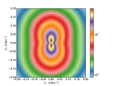
(a) Two-dimensional power spectrum with nearly-negligible Galileon potential wells, chosen so that at early times $\langle\delta\phi\delta\phi\rangle^{\ast}\approx 0$ on large scales. The fluctuations in this model are indistinguishable from $\Lambda\text{CDM}$.

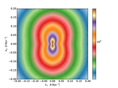
(b) Same background as Fig. 1(a), but with more significant Galileon potential wells for which $\langle\delta\phi\delta\phi\rangle^{\ast}=10M_{\mathrm{P}}^{2}\langle\Phi\Phi\rangle^{\ast}$ on large scales.

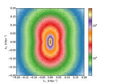
(c) Same background as Fig. 1(a), but with exaggerated Galileon potential wells for which $\langle\delta\phi\delta\phi\rangle^{\ast}=100M_{\mathrm{P}}^{2}\langle\Phi\Phi\rangle^{\ast}$ on large scales.

Figure 1: Examples of two-dimensional power spectra. The background cosmology is close to the WiggleZ best-fit combination estimated using power-spectrum data, with $\Omega_{m}=0.28$ and $f_{\text{baryon}}=0.15$. The line-of-sight velocity dispersion is taken to be $\sigma=320\,\mathrm{km}\,\mathrm{s}^{-1}$. $k_{\perp}$ and $k_{\parallel}$ represent the magnitude of momenta perpendicular and parallel to the line of sight from earth; ie., $\bm{\mathrm{{k}}}_{\parallel}=k\mu\hat{\bm{\mathrm{{x}}}}$ and $\bm{\mathrm{{k}}}_{\perp}=\bm{\mathrm{{k}}}-\bm{\mathrm{{k}}}_{\parallel}$. Only the top-right quadrant contains independent information; the other quadrants are obtained by reflections.

In current experiments the angular resolution is too coarse for this reconstruction to be performed with high accuracy. Instead, Cole, Fisher & Weinberg decomposed the angular dependence of $P_{\text{obs}}$ into multipoles Cole et al. (1994). Taking $\mathscr{P}_{{\ell}}(\mu)$ to be the Legendre polynomial of order $\ell$, the multipoles $P_{\ell}$ satisfy

$$P_{\text{obs}}(k,\mu)\equiv\sum_{\ell}P_{\ell}(k)\mathscr{P}_{{\ell}}(\mu).$$ (38)

They can be computed using orthogonality of the $\mathscr{P}_{{\ell}}$,

$$P_{\ell}(k)\equiv\frac{2\ell+1}{2}\int_{-1}^{+1}\mathrm{d}\mu\;P_{\text{obs}}(k,\mu)\mathscr{P}_{{\ell}}(\mu).$$ (39)

In §IV.3 we will see that this prescription requires modifications to account for anisotropic scaling due to the Alcock–Paczynski effect.

Within the Gaussian model only even multipoles can be nonzero, because $P_{\text{obs}}$ is a function of $\mu^{2}$. The monopole $P_{0}$ is the angle-averaged power spectrum, which was used in the analysis of Ref. Parkinson et al. (2012).

Information content.—Each multipole blends information from the $\langle\delta\delta\rangle$, $\langle\theta\delta\rangle$ and $\langle\theta\theta\rangle$ power spectra and therefore contains an admixture of the information on the force laws and number of dynamically relevant potentials carried by these correlation functions. The relative normalizations described in (13a)–(13c) fix the amplitudes of the $P_{\ell}$ as a function of scale. Also, because different combinations of correlation functions contribute to each multipole at fixed $k$, decorrelation of the $\delta$ and $\theta$ two-point functions will modify the relative normalization of the $P_{\ell}$.

IV.2 Screening and validity of linear theory

The formalism developed in §§II–III applies only to linear order in the fluctuations. When comparing its predictions to data we must be careful to exclude any modes for which nonlinear effects may have been important.

In a $\Lambda\text{CDM}$ model this is not difficult, because at any redshift there is a fixed scale beyond which structure has become nonlinear. In a modified gravity the situation may be different. In the Galileon model there is a ‘Vainshtein effect’, in which non-linear behaviour of the field $\phi$ suppresses fifth-forces in the vicinity of large mass concentrations. On a flat background the transition from unscreened to screened fifth-forces occurs roughly at the Vainshtein radius Vainshtein (1972); Nicolis et al. (2009); Burrage and Seery (2010)

$$R_{\mathrm{v}}\equiv\frac{1}{\Lambda}\Big{(}\frac{c_{3}M_{\mathrm{c}}}{2\pi c_{2}^{2}|M|}\Big{)}^{1/3}.$$ (40)

In our calculation we retain $\delta\phi$ only to first order. Therefore our formalism can not account for this Vainshtein effect. This should not be confused with the cosmological Vainshtein effect discussed in §III.2, which is a property of the background evolution.

Because this scale (40) depends on the source mass $M_{\mathrm{c}}$, the question of whether a fixed physical scale experiences screened or unscreened fifth forces throughout the survey volume depends on the realization of the density fluctuation within it—in particular, on the most massive condensation. Determining the smallest scale on which linear theory continues to apply then becomes a probabilistic exercise requiring the methods of extreme-value statistics. Even worse, the smallest unscreened scale may depend on the Lagrangian parameters and can therefore vary over parameter space.

In the cubic Galileon model these difficulties can be evaded. Inspection of (28) shows that the cosmological Vainshtein effect corresponds to the approximate rescalings

$$\Lambda\mapsto\Lambda D_{2}^{1/2},\quad M\mapsto MD_{2}^{1/2}.$$ (41)

Therefore, on the background (24), the Vainshtein radius is rescaled by a factor

$$R_{\mathrm{v}}\mapsto R_{\mathrm{v}}/D_{2}^{2/3}.$$ (42)

It can be checked that this gives

$$R_{\mathrm{v}}^{3}=\frac{1}{72\pi}\frac{c_{3}}{c_{2}^{2}}\frac{M_{\mathrm{c}}}{\rho_{m}}\sim\frac{M_{\mathrm{c}}}{\rho_{m}},$$ (43)

which is independent of the self-interaction scale $\Lambda$ and the coupling $M$. Assuming $c_{2}\sim c_{3}$ so that there are no hierarchies in the Galileon sector, it depends only on the source mass and the background matter density. This conclusion would be spoiled in a more general Galileon model where the cosmological and conventional Vainshtein effects scale differently with $\Lambda$ and $M$ if they are controlled by different $\mathcal{L}_{i}$.

For a source of density $\rho_{\mathrm{c}}$ and radius $R_{\mathrm{c}}$, Eq. (43) gives

$$R_{\mathrm{v}}=\left(\frac{1}{54}\frac{c_{3}}{c_{2}^{2}}\frac{\rho_{\mathrm{c}}}{\rho_{m}}\right)^{1/3}R_{\mathrm{c}}\sim\left(\frac{\rho_{\mathrm{c}}}{\rho_{m}}\right)^{1/3}R_{\mathrm{c}},$$ (44)

and therefore $R_{\mathrm{v}}\sim R_{\mathrm{c}}$ unless $\rho_{\mathrm{c}}$ is very different from the cosmological average $\rho_{m}$. On cluster scales the density concentration is not very large and we can expect the linearized analysis to apply on all scales which are safely larger than the clusters themselves. We sketch this situation in Fig. 2.

Figure 2: Galaxy pairs separated by short distances (eg. within a dense cluster environment) are screened by the Vainshtein mechanism. Galaxies with larger separations (eg. distant cluster members interacting with the central condensation) are unscreened, and therefore experience the effects of the fifth forces. In the WiggleZ survey most galaxies are of the second kind.

In practice we use data for wavenumbers $k\leqslant 0.2h/\text{Mpc}$ corresponding to a smallest physical scale of roughly $31h^{-1}\,\text{Mpc}$. An alternative proposal, where the calculated power spectrum is inverse-weighted by local density to measure an ‘unscreened power spectrum’, has recently been suggested by Lombriser, Simpson & Mead Lombriser et al. (2015).

IV.3 Numerical procedure

Baryonic effects.—We evolve Eqs. (2a)–(2b), (3a)–(3b) and (27a)–(27c) for different wavenumbers to construct the transfer functions ${T_{{j}}}^{{i}}$ defined in §II.2. These equations do not account for a separate baryonic component, which would require a numerical Boltzmann code including the effect of Galileon fluctuations. Instead, we model the effect of baryon suppression in the density contrast using a version of the fitting formulae given by Eisenstein & Hu Eisenstein and Hu (1998, 1997). This is implemented by constructing new transfer functions $\mathsf{T}(k)=T(k/\Gamma_{\text{eff}})$, where $\Gamma_{\text{eff}}$ is defined by Eq. (16) of Ref. Eisenstein and Hu (1997). We neglect the density of neutrinos and take the epoch of matter–radiation equality and the drag epoch to be those measured by Planck, viz. $z_{\text{eq}}=3403$ and $z_{\text{drag}}=1059.25$. The baryon fraction is fixed to be $f_{\text{baryon}}=0.15$. We do not include the effect of baryon acoustic oscillations.

Eisenstein & Hu’s formulae were calibrated by comparison to a Boltzmann code which assumed a $\Lambda\text{CDM}$ cosmology. They are unlikely to remain quantitatively accurate if the Galileon density constitutes a nonnegligible fraction of the energy budget of the universe or if Galileon forces become very significant.

Growth rates.—To accurately predict the normalization of the multipoles $P_{\ell}$ we require a reliable estimate of the relative relationship between $\delta$ and $\theta$. We assume that the linear-theory calculation gives a reliable prediction for the growth rates associated with infall into the Newtonian and Galileon potential wells, given by $f_{\text{eff}}^{\Phi}$ and $f_{\text{eff}}^{\phi}$ [see Eqs. (12a)–(12b)]. We estimate the velocity transfer functions including baryonic effects using ${\mathsf{T}_{\theta}}^{\Phi}=f_{\text{eff}}^{\Phi}{\mathsf{T}_{\delta}}^{\Phi}$ and ${\mathsf{T}_{\theta}}^{\delta\phi}=f_{\text{eff}}^{\phi}{\mathsf{T}_{\delta}}^{\delta\phi}$, where ${\mathsf{T}_{\delta}}^{\Phi}$ and ${\mathsf{T}_{\delta}}^{\delta\phi}$ are the Eisenstein & Hu transfer functions discussed above. The modified transfer functions ${\mathsf{T}_{\delta}}^{\Phi}$, ${\mathsf{T}_{\delta}}^{\delta\phi}$, ${\mathsf{T}_{\theta}}^{\Phi}$ and ${\mathsf{T}_{\theta}}^{\delta\phi}$ are used to produce our final power spectra.

CMB spectrum.—We do not use microwave background measurements except to fix the normalizations $A_{\Phi}$ and $A_{\phi}$. In particular we do not attempt to compute the microwave background angular power spectrum. This could receive corrections if the Galileon fluctuations are significant around the time of last scattering, but we leave a detailed analysis for future work.

IV.4 WiggleZ Dark Energy Survey

The WiggleZ Dark Energy Survey at the Australian Astronomical Observatory was designed to extend the study of large-scale structure to redshifts $z>0.5$, complementing SDSS observations at lower redshifts. The survey began in August 2006 and completed observations in January 2011. It has obtained of order 200,000 redshifts for UV-bright emission-line galaxies, covering close to 1000 square degrees of equatorial sky. The design of the survey and its selection function are described in Ref. Drinkwater et al. (2010).

Multipole power spectra.—The first three multipole power spectra (the monopole $P_{0}$, quadrupole $P_{2}$ and hexadecapole $P_{4}$) have been determined in three overlapping redshift bins, $0.2<z<0.6$, $0.4<z<0.8$ and $0.6<z<1.0$, and for six separated areas of the sky. These correspond to right ascensions of 1-hr, 3-hr, 9-hr, 11-hr, 15-hr and 22-hr on the celestial sphere, matching the regions observed by the survey. The effective redshifts of these bins are $z_{\text{eff}}=[0.43,0.6,0.78]$.

In this section we show that these multipole power spectra can be used to obtain constraints on the matter coupling $M$ and depth of the primordial potential wells in the cubic Galileon model. Our numerical procedure, described in §IV.3, is not exact and therefore our constraints will not be optimal. We intend them as a proof of principle. A better analysis could be performed with suitable inclusion of baryonic effects and modelling of the microwave background power spectrum.

We use only the lowest and highest redshift bins for which the redshift ranges are separate and non-overlapping. Correlation of bins between different redshifts and regions is assumed to be negligible. However, correlations between the multipole moments in the same bin are important. The covariance matrix for the three multipole power spectra has been estimated using mock catalogues generated by the Comoving Lagrangian approach Tassev et al. (2013) in a similar way to those described in Ref. Kazin et al. (2014). Full details of these simulations are given in Ref. Koda et al. (2016).

Alcock–Paczynski effect.—To convert redshift-space measurements of galaxy positions into an estimated power spectrum requires a fiducial cosmological model with which to translate observed angles and redshifts into distances. When comparing the power spectrum predicted by a given model to the observed power spectrum we must account for discrepancies between the model and this fiducial cosmology. This may introduce artificial anisotropies that confuse the extraction of redshift-space distortions. To account for this effect we introduce anisotropic scaling factors $a_{\perp}$, $a_{\parallel}$ that satisfy Tegmark et al. (2006); Reid et al. (2010); Swanson et al. (2010)

$$a_{\perp} \equiv D_{A}(z)/\hat{D}_{Z}(z)$$ (45a)

$$a_{\parallel} \equiv\hat{H}(z)/H(z),$$ (45b)

where $D_{A}$ is the angular diameter distance in the model, and $H$ is its Hubble rate; the hatted quantities $\hat{D}_{A}$ and $\hat{H}$ are the corresponding values in the fiducial model. Ballinger et al. showed that we should rescale $k$ and $\mu$ to new values $k^{\prime}$ and $\mu^{\prime}$ Ballinger et al. (1996),

$$k^{\prime} \equiv\frac{k}{a_{\perp}}\bigg{[}1+\mu^{2}\left(\frac{a_{\perp}^{2}}{a_{\parallel}^{2}}-1\right)^{1/2}\bigg{]}$$ (46a)

$$\mu^{\prime} \equiv\frac{\mu a_{\perp}}{a_{\parallel}}\bigg{[}1+\mu^{2}\left(\frac{a_{\perp}^{2}}{a_{\parallel}^{2}}-1\right)^{-1/2}\bigg{]}.$$ (46b)

The multipole power spectra defined in Eq. (39) should be computed using $k^{\prime}$ and $\mu^{\prime}$,

$$P_{\ell}(k)\equiv\frac{2\ell+1}{2a_{\perp}^{2}a_{\parallel}}\int_{-1}^{1}\mathrm{d}\mu\;P_{\text{obs}}(k^{\prime},\mu^{\prime})\mathscr{P}_{{\ell}}(\mu).$$ (47)

Even after this rescaling has taken place we must account for incompleteness in the survey volume due to the observing strategy. This requires convolution with the survey window function. For example, incompleteness may be caused by the presence of bright stars which obscure galaxies. If uncorrected these holes can introduce fake large-scale structure into the survey. Including the effect of the window function yields

$$P^{\text{con}}_{\ell_{i}}(k_{i},z_{\text{eff}})\equiv\sum_{j}W_{ij}(z_{\text{eff}})P_{\ell_{j}}\big{[}k_{j},z_{\text{eff}}\big{]},$$ (48)

where $P^{\text{con}}_{\ell}(k_{i},z_{\text{eff}})$ is the measured multipole power spectrum, and the indices $i$ and $j$ run over all combinations of multipoles $\ell$ and wavenumbers $k$ measured by the survey. The matrix $W_{ij}$ encodes details of the window function.

Model likelihood.—The final likelihood $\mathscr{L}$ is calculated by summing over regions, redshift bins, and multipole power spectra,

$$-2\ln\mathscr{L}=\sum_{\begin{subarray}{c}\text{redshifts $z$}\\ \text{regions $r$}\end{subarray}}\bm{\mathrm{\delta}}_{r,z}^{\mathsf{T}}\bm{\mathrm{C}}^{-1}_{r,z}\bm{\mathrm{\delta}}_{r,z},$$ (49)

where $\bm{\mathrm{\delta}}_{r,z}$ is the difference between the measured and predicted values of the multipole power spectra,

$$\bm{\mathrm{\delta}}_{r,z}\equiv\bm{\mathrm{P}}^{\text{mod}}_{z}-\bm{\mathrm{P}}^{\text{data}}_{r,z}.$$ (50)

In this equation, $\bm{\mathrm{P}}^{\text{mod}}_{z}$ is a vector of the multipole power spectra $(P_{0},P_{2},P_{4})$ predicted at redshift $z$ by the model in question—rescaled and evaluated at shifted wavenumbers as described in (48); $\bm{\mathrm{P}}^{\text{data}}_{r,z}$ is a similar vector of multipole power spectra estimated from the survey in region $r$ and redshift bin $z$; and $\bm{\mathrm{C}}_{r,z}$ is the covariance matrix for $r$ and $z$, accounting for covariances between the different multipole power spectra. The region label $r$ runs over all regions in the survey, and $z$ runs over all redshift bins.

Determination of $b$ and $\sigma$.—The undetermined parameters are the bias $b$, which may be a function of redshift, and the line-of-sight velocity dispersion $\sigma$. We determine $b$ by performing a maximum-likelihood estimate in each redshift bin, allowing $b$ to vary between $0.4$ and $1.8$. We determine $\sigma$ in a similar way, although it is not taken to be redshift dependent. We allow it to vary between $50\,\mathrm{km}\,\mathrm{s}^{-1}$ and $650\,\mathrm{km}\,\mathrm{s}^{-1}$. The best-fit values of the bias typically depend on $\sigma$.

V Results

In Fig. 3 we plot $1\sigma$, $2\sigma$ and $3\sigma$ best-fit regions in the $(\Omega_{m},M)$ plane for a range of models with different relative depths of the Newtonian and Galileon potential wells.

Self-interaction scale.—We choose $\Lambda=1.05\times 10^{16}H_{0}$ which enables a ‘cosmological Vainshtein’ solution to exist [see (24)]; on this solution, our results are nearly independent of $\Lambda$ at fixed $M$. The principal effect of varying $\Lambda$ is to decrease the acceptable range of $M$. Because increasing $\Lambda$ implies that (26) can be invalidated more easily, the Galileon departs more quickly from the cosmological Vainshtein solution. After departure, the quantity $|\phi/M|$ which determines the importance of quantum corrections to the matter coupling typically becomes of order unity, signalling that the model of §III becomes untrustworthy due to uncontrollable loop corrections. Therefore, as $\Lambda$ increases the range of $M$ which maintain $|\phi/M|\ll 1$ throughout the evolution becomes smaller.

For values of $|M|\lesssim M_{\mathrm{P}}$ (which covers the entire region plotted in Figs. 3(a), 3(c), 3(e), and 3(g)), the linear Galileon fifth-force is stronger than gravity. One might have expected this region to be immediately excluded due to excessive fifth forces. However, one must remember the cosmological Vainshtein mechanism: this keeps the background close to $\Lambda\text{CDM}$ and suppresses Galileon forces until the mean cosmic energy density is sufficiently low. If $|M/M_{\mathrm{P}}|$ is not too small, this means that fifth-force effects do not become strong until comparatively late.

Dependence on $\xi$.—In Fig. 3(a) we set $\xi\approx 0$, making the primordial Galileon potentials negligible. With this choice the initial conditions are indistinguishable from $\Lambda\text{CDM}$. The best fit region is centred on $\Omega_{m}\sim 0.25$, with the coupling constrained to satisfy $|M|\gtrsim 5\times 10^{-3}M_{\mathrm{P}}$. This lies just above the region (bounded by the blue contour) where loop corrections become important. Increasing $\Lambda$ would move the contour almost rigidly up the plot. The preference for a slightly low value of $\Omega_{m}$ is a feature of the WiggleZ multipole dataset, and is not connected with our modified-gravity model.

In Fig. 4 we plot the different measures of the growth factor $-\langle\theta\delta\rangle/\langle\delta\delta\rangle$ and $-\langle\theta\theta\rangle/\langle\theta\delta\rangle$ discussed in §II.2, for each value of $\xi$ appearing in Fig. 3. We measure these at $z=0.44$ in a model with $\Omega_{m}=0.25$, $\Lambda=1.05\times 10^{16}H_{0}$ and $M=-6\times 10^{-3}M_{\mathrm{P}}$ (marked by the green diamonds in Fig. 3). This lies near the bottom of the $1\sigma$ region in Fig. 3(a), and its fit becomes increasingly poor as $\xi$ increases.

Inspection of Fig. 4(a) shows that when $\xi\approx 0$ the velocity bias is precisely deterministic; there is no evidence for a second set of dynamically relevant potential wells. The constraint on $M$ arises from modifications to $f_{\text{eff}}^{\Phi}$, which become relevant only at small values of $|M/M_{\mathrm{P}}|$ where the Galileon strongly modifies the $\Lambda\text{CDM}$ background. This explains the nearly $M$-independent structure in Fig. 3(a). Throughout the $1\sigma$ region the force law is very close to Newtonian gravity, with an effective growth parameter $f_{\text{eff}}\approx 0.68$.

In Figs. 3(c) and 4(b) we plot the best-fit regions and growth factors in a model with $\xi=0.01$. In this case the constraint on $M$ strengthens slightly, so that $M=-6\times 10^{-3}M_{\mathrm{P}}$ is now on the boundary of the $3\sigma$ region. Fig. 4(b) shows that $\langle\theta\theta\rangle$, $\langle\theta\delta\rangle$ and $\langle\delta\delta\rangle$ are still closely correlated; the effective growth rates measured from different combinations of the two-point functions are nearly equal. Therefore matter concentrations and large-scale flows are still mostly associated with infall into the same set of potential wells, although these are now an admixture of Newtonian and Galileon contributions. As a result of this mixing the effective force driving matter into the potential wells has received a scale-dependent renormalization, implying a departure from the $1/r^{2}$ force law. This modification drives the weakening fit with increasing $\xi$. Clearly the effect of the second set of potential wells is very significant, even though we do not observe strong stochastic effects associated with matter moving between different combinations of them.

In Figs. 3(e) and 4(c) we plot results for the case $\xi=0.1$. The model is now excluded at more than $3\sigma$. The amplitude of the scale-dependence in the growth rate becomes larger, implying stronger departures from the $1/r^{2}$ force law, and a small amount of decorrelation becomes visible. Of the four cases exhibited in the plot, this model shows the largest decorrelation although it is still modest—of order $0.5\%$. In Figs. 3(g) and 4(d) we exhibit the case of equal potential wells, $\xi=1$. In this case the scale-dependence of the force law continues to grow stronger, but the decorrelation decreases slightly. This occurs because scale-dependence is driven entirely by the Galileon contribution, and as it becomes dominant the power spectra $\langle\theta\theta\rangle$, $\langle\theta\delta\rangle$ and $\langle\delta\delta\rangle$ will again become completely correlated.

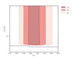
(a) Irrelevant Galileon potential wells, $\xi\approx 0$.

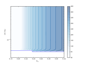
(b) Best-fit pairwise velocity dispersion $\sigma$ for Fig. 3(a).

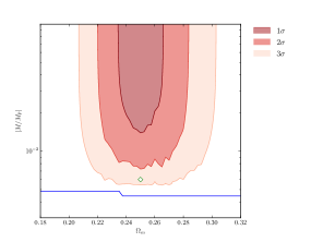
(c) Marginal Galileon potential wells, $\xi=0.01$.

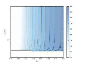
(d) Best-fit pairwise velocity dispersion $\sigma$ for Fig. 3(c).

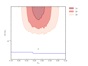
(e) Relevant Galileon potential wells, $\xi=0.1$.

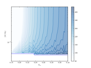
(f) Best-fit pairwise velocity dispersion $\sigma$ for Fig. 3(e).

(g) Equal Galileon potential wells, $\xi=1$.

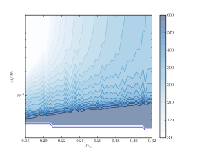
(h) Best-fit pairwise velocity dispersion $\sigma$ for Fig. 3(g).

Figure 3: Likelihoods and best-fit values for the pairwise velocity dispersion $\sigma$ for cubic Galileon model. $\xi$ measures the relative depth of the Newtonian and Galileon potential wells on large scales and was defined in Eq. (32). We exclude the region below the blue contour because $|\phi/M|$ becomes close to unity, implying that corrections to the matter coupling due to matter loops become uncontrollably large. The pairwise velocity dispersion is measured in $\mathrm{km}\,\mathrm{s}^{-1}$; see Eq. (35). Growth factors for the model indicated by the green diamond are given in Fig. 4.

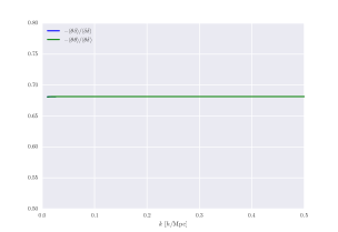
(a) Irrelevant Galileon potential wells, $\xi\approx 0$.

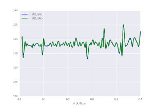
(b) Marginal Galileon potential wells, $\xi=0.01$.

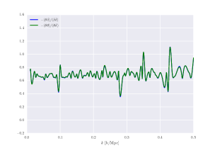
(c) Relevant Galileon potential wells, $\xi=0.1$.

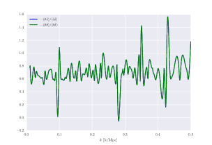
(d) Equal Galileon potential wells, $\xi=1$.

Figure 4: Effective growth rates measured in our numerical integrations at $z=0.44$ from the ratios $-\langle\theta\delta\rangle/\langle\delta\delta\rangle$ and $-\langle\theta\theta\rangle/\langle\theta\delta\rangle$. We have taken $\Omega_{m}=0.25$, $\Lambda=1.05\times 10^{16}H_{0}$ as in Fig. 3, and $M=-6\times 10^{-3}M_{\mathrm{P}}$. This model corresponds to the diamond in Fig. 3. The parameter $\xi$ measuring the relative depth of the primordial Newtonian and Galileon potential wells is defined in Eq. (32). The effective growth rates measured from the different 2-point functions are equal when $\theta$ is totally correlated with $\delta$, making the bias deterministic.

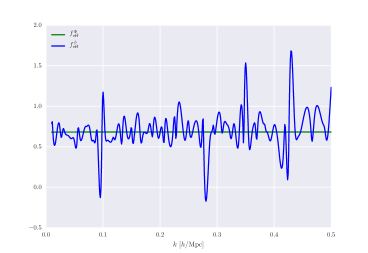
Figure 5: Growth factors $f_{\text{eff}}^{\Phi}$ and $f_{\text{eff}}^{\phi}$ measured from our simulations at $z=0.44$ [defined in Eqs. (12a)–(12b)]. The model is the same as Fig. 4. The Newtonian value is $f_{\text{eff}}^{\Phi}\approx 0.68$, matching the $\Lambda\text{CDM}$ prediction $\Omega_{m}(z)^{0.55}$.

Oscillations.—In Fig. 5 we plot the growth factors $f_{\text{eff}}^{\Phi}$ and $f_{\text{eff}}^{\phi}$ in this model; the scenarios shown in Fig. 4 are weighted averages of these. We see that $f_{\text{eff}}^{\Phi}$ is smooth while $f_{\text{eff}}^{\phi}$ is highly oscillatory. These oscillations are driven by rapid fluctuations in the evolution of the Galileon field, which would invalidate the quasi-static approximation (see §II.1).

We have verified that the oscillation pattern is stable against changes in the choice of numerical solver (LSODA, VODE and a simple Dormand–Prince 4^th/5^th-order stepper), and therefore we believe these oscillations to be real features of the model. Had we imposed the quasi-static approximation we would not have resolved them individually; instead, we expect that the solution would predict a local average. Observations are typically sensitive only to local averages of this kind, because they must aggregate over a range of angles and wavenumbers to increase signal-to-noise in each $(k,\mu)$ bin. This washes out individual features.

For the same reason the existence of these oscillations does not immediately falsify the model, even though current observations are consistent with smooth power spectra. It is possible that oscillations of this kind could be detected by a survey such as DESI that covers much larger volumes Aghamousa et al. (2016).

VI Conclusions

Summary of results.—In this paper we have set up a formalism to describe the relation between the $\langle\delta\delta\rangle$, $\langle\delta\theta\rangle$ and $\langle\theta\theta\rangle$ correlation functions in models where $\delta$ and $\theta$ are partially or totally decorrelated. In such models fifth-force effects cannot always be absorbed into a simple renormalization of the effective gravitational constant, and the $\langle\delta\delta\rangle$, $\langle\delta\theta\rangle$ and $\langle\theta\theta\rangle$ correlation functions may no longer be related by a fixed multiplicative normalization. Therefore the density and velocity fields associated with a single population of tracers may exhibit ‘stochastic’ bias, depending on the combination of primordial potentials in which matter is currently concentrated and the combination into which it is moving.

We have focused on scenarios in which the background Galileon energy density is subdominant throughout the expansion history of the universe. This is the best-motivated scenario if the Galileon arises as a vestige of other physics which solves the cosmological constant problem, such as degravitation due to a graviton mass. We have demonstrated that, in these scenarios, scale-dependent renormalization of the effective force law driving cosmological mass assembly can be constrained by measurements of the low-$\ell$ multipole power spectra $P_{\ell}$ introduced by Cole, Fisher & Weinberg Cole et al. (1994). The multipole power spectra are sensitive to some of the information regarding density and velocity correlations which is contained in the two-dimensional power spectrum $P(k,\mu)$. If enough multipoles can be measured they also constrain the effects of stochasticity.

In this paper our constraints were obtained using measurements of $P_{0}$, $P_{2}$ and $P_{4}$ from the WiggleZ galaxy redshift survey. In the cubic Galileon model, which we use as a demonstration of principle, the effects of stochasticity are not large and constraints are largely driven by changes to the force law due to mass accumulating in a combination of the primordial Newtonian and Galileon potentials. We obtain an approximate bound $|M|\gtrsim 5\times 10^{-3}M_{\mathrm{P}}$ on the conformal coupling to matter in this model.

Screening effects.—The cubic Galileon model is known to have certain pathologies, including a negative energy density on the cosmological Vainshtein solution. Its merit is that, on this solution, the Vainshtein radius is independent of the model parameters and, for clusters, roughly coincides with their physical radius. This means that linear perturbation theory is trustworthy down to roughly cluster scales.

In more general models the Vainshtein radius of a cluster may be substantially larger than its physical radius. In this case linear perturbation theory must break down roughly at the Vainshtein radius, which will generally depend on the physical properties of the cluster. For such models the validity of linear theory becomes a stochastic statement, depending on the realization of the density fluctuation within a given survey volume. It is not yet clear whether this difficulty can be surmounted within an analytic calculation (perhaps using the methods of extreme value statistics), or necessarily requires recourse to $N$-body methods.

Cosmological Vainshtein mechanism.—A key role is played by the cosmological Vainshtein solution, Eq. (24). This has two effects. First, it keeps the Galileon energy density subdominant to normal matter and radiation over most of the lifetime of the universe. This enables the background cosmology to accurately track $\Lambda\text{CDM}$. Second, it suppresses fifth-forces until late times when the Galileon’s contribution to the cosmic energy budget begins to grow. It is the cosmological Vainshtein mechanism which is responsible for enabling much of the parameter space in Figs. 3(a), 3(c), 3(e) and 3(a) to be compatible with observation, even though the Galileon fifth-force is stronger than gravity everywhere in these plots.

Multiple primordial potential wells.—Figs. 3(a), 3(c), 3(e) and 3(g) show substantially different behaviour, which can be traced to the presence of a second independent set of primordial potential wells in Fig. 3(e). It is mixing with this second set of potential wells which generates the scale-dependent renormalizations of the force law seen in Fig. 4, even though $\delta$ and $\theta$ remain strongly correlated.

The phenomenology of these models therefore depends on their inflationary prehistory. If inflation seeds a distribution of Galileon potential wells which are sufficiently deep, they leave a detectable imprint on the observable power spectrum. On the other hand, if the primordial Galileon potentials are shallow (perhaps because the Galileon was heavy during inflation, or because the potentials were later erased by some form of superhorizon evolution), their effect on the power spectrum is negligible even if the matter coupling is large. Where the primordial Galileon potential wells are not negligible their influence must be taken into account to obtain quantitatively correct results, even if there is no significant decorrelation between $\delta$ and $\theta$.

Note added.—After completion of this paper, a preprint was released by Jennings & Jennings studying stochastic effects in the relation between $\theta$ and $\delta$ within Einstein gravity Jennings and Jennings (2015). This source of stochasticity would compete with any effects from mixing of independent potential wells. If it is large, identifying stochastic effects from fifth forces would therefore require its contribution to be carefully subtracted.