Synchronization in Networks of Linearly Coupled Dynamical Systems via Event-triggered Diffusions

Abstract

In this paper, we utilize event-triggered coupling configuration to realize synchronization of linearly coupled dynamical systems. Here, the diffusion couplings are set up from the latest observations of the nodes of its neighborhood and the next observation time is triggered by the proposed criteria based on the local neighborhood information as well. Two scenarios are considered: continuous monitoring, that each node can observe its neighborhood’s instantaneous states, and discrete monitoring, that each node can only obtain its neighborhood’s states at the same time point when the coupling term is triggered. In both cases, we prove that if the system with persistent coupling can synchronize, then these event-trigger coupling strategies can synchronize the system, too.

I Introduction

Synchronization of coupled dynamical systems have been widely studied over the past decades [1]-[9], which can be characterized by that all oscillators approach to a uniform dynamical behavior and generally assured by the couplings among nodes and/or external distributed and cooperative control.

In most existing works on linearly coupled dynamical systems, each node needs to gather its own state and neighbors states and update them spontaneously or in a fixed sampling rate, which may cost much. In order to reduce the sampling rate of the coupling between nodes, specific discretization is necessary. As pointed out by [10], event-based sampling was proved to possess better performance than sampling periodically in time. Hence, [11]-[12] suggested that the event-based control algorithms to reduce communication and computation load in networked coupled systems. And [12]-[19] showed that the event-based control maintains the control performance. Event-based control seems to be suitable for coupled dynamical systems with limited resources and many works addressed the event-triggered algorithms. [13] considered centralized formulation, distributed formulation event-driven strategies for multi-agent systems and proposed a self-triggered setup, by which continuous measuring of the neighbor states can be avoided. [20]-[21] studied the stochastic event-driven strategies. [14] introduced event-based control strategies for both networks of single-integrators with time-delay in communication links and networks of double-integrators. By using scattering transformation, [18] investigated the output synchronization problem of multi-agent systems with event-driven communication in the presence of constant communication delays. In some cases, event-driven strategies for multi-agent systems can be regarded as linearization and discretization process. For example, as mentioned in [15, 16], the following algorithm

$$x^{i}(t+1)=f(x^{i}(t))+c_{i}\sum_{j=1}^{m}a_{ij}(f(x^{j}(t)))$$ (1)

can be a variant of the event triggering (distributed, self triggered) model for consensus problem. In centralized control, the bound for $(t_{k+1}^{i}-t_{k}^{i})=(t_{k+1}-t_{k})$ to reach synchronization was given in the paper [15] when the coupling graph is indirected and in [16] for the directed coupling graph.

Motivated by these works, we apply the idea of event-triggered sampling scheme to the coupling configurations to realize synchronization of linearly coupled dynamical systems. Here, for each node, the coupling term is set up from the information of its local neighborhood at the last event time and the event is triggered by some criteria derived from the information of its local neighborhood. That is, once the triggering rule of node is satisfied, the coupling term of this node is updated. Thus, the coupling terms are piece-wise constant between two neighboring event times. We consider two scenarios: continuous monitoring and discrete monitoring. Continuous monitoring means that each node can observe its neighborhood’s instantaneous information, but discrete monitoring means that each node can only obtain the its neighborhood’s information at this event triggered time. As a payoff for small cost of discrete monitoring, the triggering events happen more frequently than continuous-time monitoring. For each scenario, it is shown that the proposed event-triggered strategies guarantee the performances of the nominal systems.

This paper is organized as follows. In sec. II, we propose event-trigger coupling strategies to guarantee synchronization by employing continuous monitoring. In sec. III, we consider discrete monitoring. Simulations are given in sec. IV to verify the theoretical results. We conclude this paper in sec. V.

II Continuous-time Monitoring

We consider the following network of coupled dynamical systems with piece-wise constant linear couplings:

$$\frac{dx^{i}(t)}{dt}=f(x^{i}(t))-c\sum_{j=1}^{m}L_{ij}\Gamma(x^{j}(t_{k}^{i})-x^{i}(t_{k}^{i})),$$

$$~{}~{}t_{k}^{i}\leq t<t_{k+1}^{i},~{}i=1,\cdots,m.$$ (2)

Here, $x^{i}(t)\in\mathbb{R}^{n}$ denotes the state vector of node $i$, the continuous map $f(\cdot):\mathbb{R}^{m}\to\mathbb{R}^{m}$ denotes the identical node dynamics if there is no coupling. $L=[L_{ij}]_{i,j=1}^{m}\in\mathbb{R}^{m,m}$ is the Laplacian matrix of the underlying bi-graph $\mathcal{G}=\{V,E\}$, with the node set $V$ and link set $E$: for each pair of nodes $i\neq j$, $L_{ij}=-1$ if $i$ is linked to $j$ otherwise $L_{ij}=0$, and $L_{ii}=-\sum_{j=1}^{m}L_{ij}$; the graph that we consider in this paper is undirected and connected, so $L$ is irreducible and symmetric. $c$ is the uniform coupling strength at all nodes, and $\Gamma\in\mathbb{R}^{n,n}$ denotes the inner configuration matrix. Let $0=\lambda_{1}(L)<\lambda_{2}(L)\leq\cdots\leq\lambda_{m}(L)$ be the eigenvalues of $L$ with counting the multiplicities.

The increasing triggering event time sequence $\{t_{k}^{i}\}_{k=1}^{\infty}$ (to be defined) are node-wise for $i=1,\cdots,m$. At time $t$, each node $i$ collects its neighbor’s state with respect to an identical time point $t_{k_{i}(t)}^{i}$ with $k_{i}(t)=arg\max_{k^{\prime}}\{t^{i}_{k^{\prime}}\leq t\}$.

For the node dynamics map $f$, we suppose it belong to some map class $Quad(P,\alpha\Gamma,\beta)$ for some positive definite matrix $P\in\mathbb{R}^{n,n}$, constant $\alpha\in\mathbb{R}$ and positive constant $\beta>0$, i.e.,

$$(u-v)^{\top}P\bigg{[}f(u)-f(v)-\alpha\Gamma(u-v)\bigg{]}$$

$$\leq-\beta(u-v)^{\top}P(u-v)$$ (3)

holds for all $u,v\in\mathbb{R}^{n}$. In fact, we do not need this $Quad$ condition (3) holds for all $u,v\in\mathbb{R}^{n}$ but for a region $\Omega\subset\mathbb{R}^{n}$, which is assumed to contain a global attractors of the coupling systems (2).

We highlight the basic idea behind the setup of the coupling term above. Instead of using the spontaneous state from the neighborhood to realize synchronize, an economic alternative for the node $i$ is to use the neighbor’s constant states at the nearest time point $t^{i}_{k}$ until some pre-defined event is triggered at time $t^{i}_{k+1}$; then the incoming neighbor’s information is updated by the states at $t^{i}_{k+1}$ until the next event is triggered, and so on. The event is defined based on the neighbor’s and its own states with some prescribed rule. This process goes on through all nodes in a parallel fashion.

To depict the event that triggers the next coupling time point, we introduce the following candidate Lyapunov function:

$$V(t) =-\frac{1}{2}\sum_{i=1}^{m}\sum_{j=1}^{m}L_{ij}(x^{i}(t)-x^{j}(t))^{\top}P(x^{i}(t)-x^{j}(t))$$

$$=x^{\top}(t)(L\otimes P)x(t)$$ (4)

with $x=[{x^{1}}^{\top}(t),\cdots,{x^{m}}^{\top}(t)]^{\top}\in\mathbb{R}^{nm}$ and $\otimes$ represents the Kronecker product. For a compact expression, we denote $F(x)=[f(x^{1})^{\top},\cdots,f(x^{m})^{\top}]^{\top}$. Then, the derivative of $V(t)$ along (2) is

$$\frac{d}{dt}V(t)\left|{}_{(\ref{cds})}\right.= 2x^{\top}(t)(L\otimes P)\bigg{\{}F(x(t))-\alpha(I_{m}\otimes\Gamma)x(t)$$

$$-[(cL-\alpha I_{m})\otimes\Gamma]x(t)+ce(t)\bigg{\}}$$ (5)

where $e(t)=[e_{1}^{\top}(t),\cdots,e^{\top}_{m}(t)]^{\top}$ and

$$e_{i}(t)=\sum_{j}L_{ij}\Gamma\left(x^{j}(t)-x^{j}(t_{k_{i}(t)}^{i})-x^{i}(t)+x^{i}(t_{k_{i}(t)}^{i})\right).$$

By assuming $f\in Quad(P,\alpha\Gamma,\beta)$, we have

$$\frac{d}{dt}V(t)\left|{}_{(\ref{cds})}\right.$$

$$\leq -2\beta x^{\top}(L\otimes P)x-2x^{\top}[L(cL-\alpha I_{m})\otimes(P\Gamma)]x$$

$$+2cx^{\top}(L\otimes P)e$$

$$\leq -2\beta^{\prime}x^{\top}(L\otimes P)x-2(\beta-\beta^{\prime})x^{\top}(L\otimes P)x$$

$$-2(c\lambda_{2}(L)-\alpha)x^{\top}[L\otimes(P\Gamma)]x+2cx^{\top}(L\otimes P)e$$ (6)

with any $0<\beta^{\prime}<\beta$. Pick a constant $\upsilon>0$, then

$$2x^{\top}(L\otimes P)e \leq{\upsilon}x^{\top}(L^{2}\otimes P^{2})x+\frac{1}{\upsilon}e^{\top}e$$

$$\leq{\upsilon\lambda_{m}(L)\lambda_{m}(P)}x^{\top}(L\otimes P)x+\frac{1}{\upsilon}e^{\top}e.$$ (7)

Substitute inequality (II) into (II), we have

$$\frac{d}{dt}V(t)\left|{}_{(\ref{cds})}\right. \leq-2(\beta-\beta^{\prime})V(t)-2(c\lambda_{2}(L)-\alpha)V(t)$$

$$+[-2\beta^{\prime}+{c\upsilon\lambda_{m}(L)\lambda_{m}(P)}]V(t)+\frac{c}{\upsilon}e^{\top}e.$$ (8)

Denote

$$z_{i}(t)=\sqrt{\sum_{j\neq i}(-L_{ij})(x^{j}(t)-x^{i}(t))^{\top}P(x^{j}(t)-x^{i}(t))}.$$

Then, we have $V(t)=\sum_{i=1}^{m}z_{i}^{2}(t)$.

Denote $\|\cdot\|$ the Euclidean norm, i.e., for any vector $\xi\in\mathbb{R}^{n}$, $\|\xi\|=\sqrt{\xi_{1}^{2}+\cdots+\xi_{n}^{2}}$. For a matrix $A\in\mathbb{R}^{n\times n}$, the spectral norm of $A$ is induced from Euclidean norm, i.e., $\|A\|=\sqrt{\lambda_{max}(A^{\top}A)}$. Hence, $\|A\xi\|\leq\|A\|\|\xi\|$ always holds, which will be used later as default. Moreover, $\|x\|_{P}=\sqrt{x^{\top}Px}$ for some positive definite matrix $P\in\mathbb{R}^{n,n}$. Thus, we have the following theorem

Theorem 1.

Suppose that $f\in Quad(P,\alpha\Gamma,\beta)$ with positive matrix $P$ and $\beta>0$, $c\lambda_{2}(L)>\alpha$ and $P\Gamma$ is semi-positive definite. Pick $\beta^{\prime}<\beta$. Then either one of the following two updating rules can guarantee that system (2) synchronizes:

1. Set $t^{i}_{k+1}$ as the time point by the rule

   $$t_{k+1}^{i}= \max_{\tau}\left\{\tau\geq t_{k}^{i}:\right.$$

   $$\left.~{}\|e_{i}(\tau)\|\leq\frac{\beta^{\prime}}{c\sqrt{\lambda_{m}(L)\lambda_{m}(P)}}z_{i}(\tau)\right\};$$ (9)

2. Set $t^{i}_{k+1}$ as the time point by the rule

   $$t_{k+1}^{i}=\max\left\{\tau\geq t_{k}^{i}:~{}\|e_{i}(\tau)\|\leq a\exp{(-b\tau)}\right\}.$$ (10)

Proof.

Noting that $c\lambda_{2}(L)>\alpha$ holds and $P\Gamma$ is semi-positive definite. By (II), we have

$$\frac{d}{dt}V(t)\left|{}_{(\ref{cds})}\right.\leq -2(\beta-\beta^{\prime})V(t)+[c\upsilon\lambda_{m}(L)\lambda_{m}(P)$$

$$-2\beta^{\prime}]V(t)+\frac{c}{\upsilon}\|e(t)\|^{2}$$

$$= -2(\beta-\beta^{\prime})V(t)+\sum_{i=1}^{m}[c\upsilon\lambda_{m}(L)\lambda_{m}(P)$$

$$-2\beta^{\prime}]z_{i}^{2}(t)+\sum_{i=1}^{m}\frac{c}{\upsilon}\|e_{i}(t)\|^{2}$$ (11)

holds for any $\upsilon>0$.

(1). In case of

$$\|e_{i}(t)\|^{2}\leq\frac{\upsilon}{c}[2\beta^{\prime}-c\upsilon\lambda_{m}(L)\lambda_{m}(P)]z_{i}^{2}(t)$$ (12)

for some constant $\upsilon>0$, we have

$$\frac{d}{dt}V(t)\left|{}_{(\ref{cds})}\right.\leq-2(\beta-\beta^{\prime})V.$$ (13)

This implies that $V(t)$ converges to $0$ exponentially. Note

$$\max_{\upsilon>0}\frac{\upsilon}{c}[2\beta^{\prime}-c\upsilon\lambda_{m}(L)\lambda_{m}(P)]=\frac{\beta^{\prime 2}}{c^{2}\lambda_{m}(L)\lambda_{m}(P)}.$$

Then, we take $\upsilon=\frac{\beta^{\prime}}{c\lambda_{m}(L)\lambda_{m}(P)}$, which guarantees that (9) holds.

(2). In case of

$$\|e_{i}(t)\|\leq a\exp{(-bt)},$$ (14)

we have

$$\frac{d}{dt}V(t)\left|{}_{(\ref{cds})}\right.\leq -2(\beta-\beta^{\prime})V+[c\upsilon\lambda_{m}(L)\lambda_{m}(P)$$

$$-2\beta^{\prime}]V+\frac{a^{2}cm}{\upsilon}\exp{(-2bt)}.$$

Pick $\upsilon=\frac{2\beta^{\prime}}{c\lambda_{m}(L)\lambda_{m}(P)}$. Then, we have

$$\frac{d}{dt}V(t)\left|{}_{(\ref{cds})}\right. \leq-2(\beta-\beta^{\prime})V$$

$$+\frac{a^{2}c^{2}m\lambda_{m}(L)\lambda_{m}(P)}{2\upsilon\beta^{\prime}}\exp{(-2bt)},$$ (15)

which implies that $V(t)$ converges to $0$ exponentially.

∎

In fact, in (9), if $\tau=t_{k}^{i}$ but the system does not synchronize, then the left-hand term $\|e_{i}(t_{k}^{i})\|=0$ and at least one agent has positive right-hand term, which means the next inter-event interval of one agent must be positive. While in (10), if $\tau=t_{k}^{i}$ but the system does not synchronize, the left-hand term equals $0$ and the right-hand term is positive for all nodes. Hence, the inter-event intervals of all agents are positive. But in case the derivative of $e_{i}(t)$ is sufficiently large, the inter-event interval might tends to $0$. Since the dynamics of $e_{i}(t)$ is highly related to the property of $f(\cdot)$, towards a lower-bound of the inter-event intervals, we suppose that $f(\cdot)$ is Lipschitz in the following theorem.

It should be highlighted that if $f$ is Lipschitz and $P\Gamma$ is semi-positive definite, then $f\in Quad(P,\alpha\Gamma,\beta)$ with $\beta=\frac{\alpha\lambda_{1}(P\Gamma)}{\lambda_{m}(P)}-\frac{\lambda_{m}(P)}{\lambda_{1}(P)}$. Thus, we have

Theorem 2.

Suppose $f\in Quad(P,\alpha\Gamma,\beta)$ with positive matrix $P$ and $\beta>0$, satisfies Lipschitz condition with Lipschitz constant $L_{f}$, and there exists some $\sigma$ (possibly negative) such that

$$(u-v)^{\top}P(f(u)-f(v))\geq\sigma(u-v)^{\top}P(u-v)$$ (16)

for all $u,v\in\mathbb{R}^{n}$. $c\lambda_{2}(L)>\alpha$ and $P\Gamma$ is semi-positive definite. For any $\beta^{\prime}<\beta$, any initial condition and any time $t\leq 0$, we have

1. With the updating rule (9), at least one agent has next inter-event interval, which is lower-bounded by a common constant $\tau_{O}>0$. in addition, if there exists $\varsigma>0$ such that $z_{i}^{2}(t)\geq\varsigma V(t)$ for all $i=1,\cdots,m$ and $t\geq 0$, then the next inter-event interval of every agent is strictly positive and is lower-bounded by a common constant.

2. With the updating rule (10), the next inter-event interval of every agent is strictly positive and is lower-bounded by a common constant.

Proof.

(1). Note

$$\dot{x}^{j}(t)-\dot{x}^{i}(t)= f(x^{j})-f(x^{i})-c[(L\otimes\Gamma)x(t_{k_{j}(t)}^{j})]_{j}$$

$$+c[(L\otimes\Gamma)x(t_{k}^{i})]_{i},~{}~{}~{}~{}~{}t\in[t_{k}^{i},t_{k+1}^{i}).$$

Combining with the facts that $f$ is Lipschitz and $V(t)$ is decreasing, we have

$$\|\dot{x}^{j}(t)-\dot{x}^{i}(t)\|\leq L_{f}\|x^{j}(t)-x^{i}(t)\|+c\|\Gamma\|V(t_{k}^{i}).$$ (17)

According to

$$e_{i}(t)=\sum_{j}L_{ij}\Gamma\int_{t_{k}^{i}}^{t}[\dot{x}^{j}(s)-\dot{x}^{i}(s)]ds$$ (18)

and inequality (17), we have

$$\|e_{i}(t)\|\leq \frac{1}{\sqrt{\lambda_{1}(P)}}\left(L_{f}\|\Gamma\|+mc\|\Gamma\|^{2}\right)\sqrt{2V(t_{k}^{i})}(t-t_{k}^{i}).$$ (19)

And, noting $V(t)=\sum_{i=1}^{m}z_{i}^{2}(t)$, there exists $i_{*}$ such that

$$z_{i_{*}}(t)\geq\sqrt{\frac{1}{m}V(t)}.$$ (20)

From the condition (16), (5) gives

$$\dot{V} \geq 2\sigma x^{\top}(t)(L\otimes P)x(t)-2cx^{\top}(t)[L^{2}\otimes(P\Gamma)^{s}]x(t)$$ (21)

$$+c2x^{\top}(t)(L\otimes P)e(t).$$

Noting

$$u^{\top}[L^{2}\otimes(P\Gamma)^{s}]u\leq\lambda_{m}(L)\frac{\|(P\Gamma)^{s}\|}{\lambda_{1}P)}u^{\top}[L\otimes(P)]u,$$

for all $u\in\mathbb{R}^{mn}$,

$$2x^{\top}(L\otimes P)e \geq -{\upsilon}x^{\top}(L^{2}\otimes P^{2})x-\frac{1}{\upsilon}e^{\top}e$$

$$\geq -{\upsilon\lambda_{m}(L)\lambda_{m}(P)}x^{\top}(L\otimes P)x-\frac{1}{\upsilon}e^{\top}e,$$

and event (9), (21) gives

$$\dot{V}(t)\geq\varpi V(t)$$

for all $t$ before the next triggering time, with

$$\varpi = 2\sigma-2\lambda_{m}(L)\frac{\|(P\Gamma)^{s}\|}{\lambda_{1}(P)}-\upsilon\lambda_{m}(L)\lambda_{m}(P)$$

$$-\frac{1}{\upsilon}\frac{\beta^{\prime}}{c\lambda_{m}(L)\lambda_{m}(P)}.$$

Thus, we have $V(t)\geq V(t_{k}^{i_{*}})\exp(\varpi(t-t^{i_{*}}_{k}))$. Combined with (19) and (20), this implies that for each $t\leq t^{i_{*}}_{k}+\tau_{O}$, where $\tau_{O}$ satisfies

$$\frac{\left(L_{f}\|\Gamma\|+mc\|\Gamma\|^{2}\right)\sqrt{2}}{\sqrt{\lambda_{1}(P)}}\tau_{O}=\frac{\beta^{\prime}\sqrt{\frac{1}{m}\exp(\varpi\tau_{O})}}{c\sqrt{\lambda_{m}(L)\lambda_{m}(P)}}$$

we have the inequality in (9) holds. Therefore, we have the next triggering time should be larger than $t^{i_{*}}_{k}+\tau_{O}$.

In addition, if $z_{i}^{2}(t)\geq\varsigma V(t)$ for all $i=1,\cdots,m$ and $t\geq 0$, replace (20) by

$$z_{i}(t)\geq\sqrt{\varsigma V(t)}$$ (22)

for all $i=1,\cdots,m$. Then following the same arguments after (20), we can conclude that we have the inequality in (9) holds for all $t\geq t_{k}^{i}+\tau_{O^{\prime}}$ with some positive $\tau_{O^{\prime}}$ satisfying:

$$\frac{\left(L_{f}\|\Gamma\|+mc\|\Gamma\|^{2}\right)\sqrt{2}}{\sqrt{\lambda_{1}(P)}}\tau_{O^{\prime}}=\frac{\beta^{\prime}\varsigma\sqrt{\exp(\varpi\tau_{O^{\prime}})}}{c\sqrt{\lambda_{m}(L)\lambda_{m}(P)}}.$$

(2). Under updating rule (10). By inequality (II), we get

$$V(t)\leq\rho\exp{[-2\min(b,\beta-\beta^{\prime})t]}$$

with $\rho=V(0)+\frac{a^{2}c^{2}m\lambda_{m}(L)\lambda_{m}(P)}{4v\beta^{\prime}(\beta-\beta^{\prime})}+1$. Hence, combined with (19), this gives

$$\|e_{i}(t)\|\leq \sqrt{\frac{2\rho}{\lambda_{1}(P)}}\left(L_{f}\|\Gamma\|+mc\|\Gamma\|^{2}\right)$$

$$\times\exp{[-\min(b,\beta-\beta^{\prime})t_{k}^{i}]}(t-t_{k}^{i}).$$

Therefore, (10) is guaranteed by the following inequality

$$\sqrt{\frac{2\rho}{\lambda_{1}(P)}}\left(L_{f}\|\Gamma\|+mc\|\Gamma\|^{2}\right)\exp{[-\min(b,\beta-\beta^{\prime})t_{k}^{i}]}(t-t_{k}^{i})$$

$$\leq a\exp{(-bt)}.$$

Since at time $t=t_{k}^{i}$, $e_{i}(t)=0$ holds. Based on rule (10), the next event will not trigger until $e_{i}(t)=a\exp{(-bt)}$. Thus, the inter-event intervals $\tau=t_{k+1}^{i}-t_{k}^{i}$ is lower bounded by the solution $\tau_{D}$ of the following equation

$$\sqrt{\frac{2\rho}{\lambda_{1}(P)}}\left(L_{f}\|\Gamma\|+mc\|\Gamma\|^{2}\right)\exp{[-\min(b,\beta-\beta^{\prime})t_{k}^{i}]}\tau_{D}$$

$$=a\exp{[-b(\tau_{D}+t_{k}^{i})]}.$$

It can be seen that this equation has a positive solution. This completes the proof. ∎

Remark 1.

The updating rules (9) and (10) are different but closely related to each other in some respects. It can be seen from inequalities (II) and (II) used in the derivation that the convergence behavior for (9) might be better than (10). However, it makes rule (9) more complicated than (10), since each agent should receive the message of the states of its neighborhood but rule (10) does not need. Therefore, rule (9) costs more updating times than (10). Moreover, as shown by Theorem 2, rule (10) can guarantee the positivity of the intervals to next updating time for all agents but rule (9) can only guarantee it for at least one agent at each time or for all nodes under some specific additional conditions.

III Discrete-time Monitoring

By the discrete-time monitoring strategy, each node $i$ only needs its local neighborhood’s state at time-points $t^{i}_{k}$, $k=1,2,\cdots$. By this way, the design of the next $t^{i}_{k+1}$ depends only on the local states at time $t^{i}_{k}$, other than the triggering event (9), (10), which requires the continuous time states. For early works, see [15, 16] for reference.

Consider system (2) and the candidate Lyapunov function $V(x)$ with its derivative (5). To propose a triggering criterion, which depends only on $t_{k}^{i}$ by the criterion (9) in Theorem 1, we need to estimate the bounds of $(x^{q}(t)-x^{q}(t_{k}^{l}))-(x^{i}(t)-x^{i}(t_{k}^{l}))$ for any $q,i$ with $L_{iq}\neq 0$ and $x^{i}(t)-x^{j}(t)$ for any $i\neq j$.

First, we estimate the lower-bound of $x_{i}(t)-x_{j}(t)$, which satisfies

$$\frac{d[x^{i}(t)-x^{j}(t)]}{dt}=[f(x^{i}(t))-f(x^{j}(t))]+\theta_{i}(t_{k_{i}(t)}^{i})-\theta_{j}(t_{k_{j}(t)}^{j})$$

by provided the initial values at $t^{i}_{k}$: $x^{i}(t^{i}_{k})$ and $x^{j}(t^{i}_{k})$. This can be generalized as

$$\begin{cases}\frac{du}{dt}=f(u(t))+\theta&u(0)=u_{0}\\ \frac{dv}{dt}=f(v(t))+\vartheta&v(0)=v_{0}.\end{cases}$$ (23)

Suppose that the solutions satisfy the following inequality:

$$\bigg{[}(u(t)-v(t))^{\top}{P}(u(t)-v(t))\bigg{]}^{1/{2}}\geq\varrho(t,\theta,\vartheta,u_{0},v_{0})$$ (24)

Here $\varrho$ can be regarded as the lower-bound estimation of the distance (in $P$-norm) between two trajectories:

$$\|u(t)-v(t)\|_{P}$$

$$= \bigg{\|}\int_{0}^{t}[f(u(s))-f(v(s))]ds+(\theta-\vartheta)t-(u_{0}-v_{0})\bigg{\|}_{P}.$$

To specify $\varrho$, the celebrated Gronwall-Bellman inequality is used, which can be verified straightforwardly and described as follows:

Lemma 1.

[22, 23] For a nonnegative differentiable function $x(t)$ and two continuous functions: $\alpha(t)$ and $\beta(t)$, defined on interval $[a,b]$, if

$$\dot{x}\geq\alpha(t)x(t)+\beta(t)$$

for all $t\in[a,b]$, then we have

$$x(t)\geq x(a)\exp\left(\int_{a}^{t}\alpha(s)ds\right)$$

$$+\int_{a}^{t}\beta(s)\exp\left(\int_{s}^{t}\alpha(u)du\right);$$ (25)

for two continuous functions $x(t)$ and $\beta(t)$, and an integrable function $\alpha(t)$, defined on interval $[a,b]$, if $\beta(\cdot)$ is nonnegative and

$$x(t)\leq\alpha(t)+\int_{a}^{t}\beta(s)x(s)ds$$

for all $t\in[a,b]$, then we have

$$x(t)\leq\alpha(t)+\int_{a}^{t}\alpha(s)\beta(s)\exp\left(\int_{s}^{t}\beta(u)du\right).$$ (26)

By this lemma, $\varrho$ is a nonnegative-valued continuous map and satisfies (i). $\varrho(\cdot,\theta,\theta,u_{0},u_{0})\equiv 0$; (ii). $\varrho(0,\cdot,\cdot,u_{0},u_{0})\equiv 0$. For example, assuming that condition (16) holds, we have

$$\frac{d}{dt}[(u(t)-v(t))^{\top}P(u(t)-v(t))]\left|{}_{(\ref{r2})}\right.$$

$$= 2(u-v)^{\top}P[f(u)-f(v)+\theta-\vartheta]$$

$$\geq {2\sigma}(u-v)^{\top}P(u-v)-\mu(u-v)^{\top}P(u-v)$$

$$-\frac{1}{\mu}(\theta-\vartheta)^{\top}P(\theta-\vartheta)$$

for any $\mu>0$. By the Gronwall-Bell inequality (25), we have

$$(u(t)-v(t))^{\top}P(u(t)-v(t))$$

$$\geq\exp{[({2\sigma}-\mu)t]}(u_{0}-v_{0})^{\top}P(u_{0}-v_{0})$$

$$-\frac{(\theta-\vartheta)^{\top}P(\theta-\vartheta)/\mu}{2\sigma-\mu}\bigg{\{}\exp[({2\sigma}-\mu)t]-1\bigg{\}}$$

which is positive for a small interval of $t$, starting from $0$, and $u_{0}\neq v_{0}$.

It can be seen that (16) holds for a large class of functions $f(\cdot)$. For example, if there exists some $\sigma\in\mathbb{R}$ such that

$$\{P\frac{\partial f}{\partial x}(x)\}^{s}\geq\sigma P$$ (27)

for all $x\in\mathbb{R}^{n}$ and some $\sigma\in\mathbb{R}$, then

$$(u-v)^{\top}P[f(u)-f(v)]=\int_{0}^{1}(u-v)^{\top}$$

$$\{P\frac{\partial f}{\partial x}(\lambda(v-u)+v)\}^{s}(u-v)d\lambda\geq\sigma(u-v)^{\top}P(u-v),$$

which implies (16). In particular, if the Jacobin of $f(\cdot)$ is bounded, namely, $\|{\partial f}/{\partial x}\|\geq J_{f}$ for some $J_{f}>0$, then we have

$$\{P\frac{\partial f}{\partial x}(y)\}^{s}\geq-J_{f}\|P\|,$$

which implies $\sigma=-J_{f}\frac{\|P\|_{2}}{\lambda_{\min}(P)}$ in (27).

Second, we consider the differential equations (23) and suppose that the solutions of (23) satisfy the following inequality:

$$\|(u(t)-u_{0})-(v(t)-v_{0})\|\leq\rho(t,\theta,\vartheta,u_{0},v_{0}),$$ (28)

where $\rho$ is nonnegative-valued continuous map that depends on the node dynamics map $f(\cdot)$, the initial value $u_{0},v_{0}$ and inputs $\theta,\vartheta$, and satisfies $\rho(0,\cdot,\cdot,\cdot,\cdot)\equiv 0$. Geometrically, $\rho$ is an upper-bound estimation of the difference between the displacements of two trajectories of (23) with respect to their initial locations,

$$\|(u(t)-u_{0})-(v(t)-v_{0})\|$$

$$= \left\|\int_{0}^{t}[f(u(s))-f(v(s))]ds+(\theta-\vartheta)t\right\|.$$

For example, if $f(\cdot)$ is Lipschitz (on the two trajectories): $\|f(u(s))-f(v(s))\|\leq L_{f}\|u(s)-v(s)\|$ for all $s\geq 0$, then we have

$$\|(u(t)-u_{0})-(v(t)-v_{0})\|$$

$$\leq L_{f}\int_{0}^{t}\|(u(s)-u_{0})-(v(s)-v_{0})\|ds$$

$$+(\|\theta-\vartheta\|+L_{f}\|u_{0}-v_{0}\|)~{}t.$$

By the Gronwall inequality (26), we have

$$\|(u(t)-u_{0})-(v(t)-v_{0})\|$$

$$\leq \frac{(\|\theta-\vartheta\|+L_{f}\|u_{0}-v_{0}\|)}{L_{f}}[\exp(L_{f}t)-1].$$ (29)

It can be seen that the upper-bound equals to zero if $t=0$.

It can be seen that the estimation of $\rho$ and $\varrho$ substantially depends on the form of $f(\cdot)$. There might not be a unified approach to give precise estimation for general $f(\cdot)$ but might be done case by case. Therefore, an efficient but cost way is to use integrators that simulate the node dynamics of $\dot{u}=f(u)+\theta$ as the generators of $\rho$ and $\varrho$. These generators are independent of the states of the nodes and so parallel to the networked systems. Figs. 1 and 2 show the configurations of the generators of $\rho$ and $\varrho$ respectively.

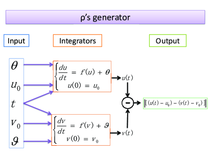
Figure 1: $\rho$ generator.

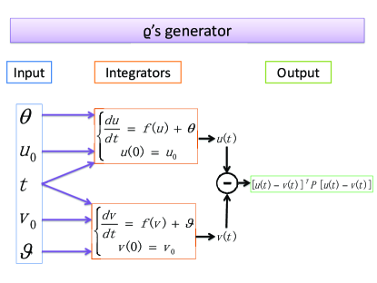
Figure 2: $\varrho$ generator.

Let

$$\theta^{i}_{k}=-c\sum_{j=1}^{m}L_{ij}(x^{j}(t^{i}_{k})-x^{i}(t^{i}_{k})),$$

$$\theta_{k_{j}(t)}^{j}=-c\sum_{l=1}^{m}L_{jl}[x^{l}(t^{j}_{k_{j}(t)})-x^{j}(t^{j}_{k_{j}(t)})]$$

Then, for $\tau\geq t^{i}_{k}$, we have

$$\|e_{i}(\tau)\|\leq\sum_{q\neq i}(-L_{iq})\|\Gamma\|\rho(\tau-t_{k}^{i},\theta^{i}_{k},\theta_{k_{q}(\tau)}^{q},x^{i}(t_{k}^{i}),x^{q}(t^{i}_{k})),$$

$$z_{i}(\tau)\geq\sqrt{\sum_{j\neq i}(-L_{ij})\varrho^{2}(\tau-t_{k}^{i},\theta^{i}_{k},\theta_{k_{j}(\tau)}^{j},x^{i}(t_{k}^{i}),x^{j}(t^{i}_{k}))}.$$

With these assumptions and Theorem 1, we have the following result.

Theorem 3.

Suppose that $f\in Quad(P,\alpha\Gamma,\beta)$ with positive matrix $P$ and $\beta>0$ such that $P\Gamma$ is semi-positive definite. $c\lambda_{2}(L)>\alpha$. For any positive $\beta^{\prime}<\beta$, set $\xi^{i}_{k}$ by:

$$\xi^{i}_{k}=\max\bigg{\{} \xi:~{}\sum_{q\neq i}(-L_{iq})\|\Gamma\|\rho(\xi,\theta^{i}_{k},\theta_{k_{q}(\xi+t_{k}^{i})}^{q},x^{i}(t_{k}^{i}),x^{q}(t^{i}_{k}))$$

$$\leq\frac{\beta^{\prime}}{c\sqrt{\lambda_{m}(L)\lambda_{m}(P)}}\bigg{[}\sum_{q\neq i}(-L_{iq})\varrho^{2}(\xi,\theta^{i}_{k},\theta_{k_{j}(\xi+t_{k}^{i})}^{j},$$

$$~{}~{}~{}~{}~{}~{}~{}~{}~{}~{}~{}~{}~{}~{}~{}~{}~{}~{}~{}~{}~{}~{}~{}~{}~{}~{}~{}x^{i}(t_{k}^{i}),x^{j}(t^{i}_{k}))\bigg{]}\bigg{\}}.$$ (30)

The event timing $\{t^{i}_{k}\}$ are set by the following scheme:

1. Initialization: $t_{0}^{i}=0$ for all $i=1,\cdots,m$;

2. For node $i$, set $\xi^{i}_{k}$ via its neighbor’s and its own current states and diffusion by (30);

3. If one of its neighbors, for example, $j$, triggers at $t=t^{j}_{k^{\prime}+1}$ ($k^{\prime}$ is the latest event at node $j$ before $t$), then replace $\theta^{j}_{k^{\prime}}$ by $\theta^{j}_{k^{\prime}+1}$ in (30) and go to Step 2;

4. Let $t^{i}_{k+1}=t^{i}_{k}+\xi^{i}_{k}$, the event triggers at node $i$ by changing $t^{i}_{k}$ in (2) to $t^{i}_{k+1}$.

Then, system (2) synchronizes.

The proof of this theorem can be derived by using (9) in Theorem 1 directly.

Remark 2.

Firstly, if node $i$ has a neighbor $j$ satisfying $x^{j}(t^{i}_{k})\neq x^{i}(t^{i}_{k})$, then $\xi_{k}^{i}$ in (30) is well defined. In fact, in (30), if $\xi=0$, the left-hand side of the inequality in (30) equals zero while the right-hand side is nonzero. Therefore, by the continuous dependence of the parameters in the system (2), (30) has indeed a positive maximum $\xi$.

Secondly, each node $i$ needs to know the states of itself and its neighbors. In details, when one node $j$ is triggered, it sends off its new coupling terms, $\theta_{j}(t^{j}_{k_{j}(t)})$, to all its neighbors for their updating the estimation of $\xi^{i}_{k}$ for their next updating times.

Remark 3.

In case that $x^{j}(t^{i}_{k})=x^{i}(t^{i}_{k})$ for all neighbors $j$ of node $i$, both left and right sides equal zero, which might lead to a Zeno behavior. To avoid the Zeno behavior, we provide a triggering event, which depends only on $t_{k}^{i}$ by the rule (10) in Theorem 1. Here, we only need to estimate the bounds of $(x^{q}(t)-x^{q}(t_{k}^{l}))-(x^{i}(t)-x^{i}(t_{k}^{l}))$ for any $q,i$ with $L_{iq}\neq 0$. Note

$$(x^{q}(t)-x^{q}(t_{k}^{l}))-(x^{i}(t)-x^{i}(t_{k}^{l}))$$

$$= \int_{t_{k}^{l}}^{t}\left[f(x^{q}(s))-f(x^{i}(s))+\theta_{k_{q}(s)}^{q}-\theta^{i}_{k}\right]ds.$$

Combing with $\|\theta^{i}_{k}-\theta_{k_{q}(s)}^{q}\|\leq M$, where $M>0$ is some constant, we suppose that the solutions of (23) satisfy the following inequality:

$$\|(u(t)-u_{0})-(v(t)-v_{0})\|\leq\rho_{1}(t,u_{0},v_{0}).$$ (31)

Then, for $\tau\geq t^{i}_{k}$, we have

$$\|e_{i}(\tau)\|\leq\sum_{j\neq i}(-L_{ij})\|\Gamma\|\rho_{1}(\tau-t_{k}^{i},x^{i}(t_{k}^{i}),x^{j}(t^{i}_{k})).$$

Theorem 4.

Suppose that $f\in Quad(P,\alpha\Gamma,\beta)$ with positive matrix $P$ and $\beta>0$ such that $P\Gamma$ is semi-positive definite. $c\lambda_{2}(L)>\alpha$. For any positive $\beta^{\prime}<\beta$, set inter-event interval $\xi^{i}_{k}$ by:

$$\xi^{i}_{k}=\max\bigg{\{} \xi:~{}\sum_{j\neq i}(-L_{ij})\|\Gamma\|\rho_{1}(\xi,x^{i}(t_{k}^{i}),x^{j}(t^{i}_{k}))$$

$$\leq a\exp{[-b(\xi+t_{k}^{i})]}\bigg{\}}.$$ (32)

The event times $\{t^{i}_{k}\}$ are set by the following scheme:

1. Initialization: $t_{0}^{i}=0$ for all $i=1,\cdots,m$;

2. For node $i$, search $\xi^{i}_{k}$ via its neighbor’s and its own current states by (30);

3. Triggers node $i$ by changing $t^{i}_{k}$ in (2) to $t^{i}_{k+1}=t^{i}_{k}+\xi^{i}_{k}$,.

Then, system (2) synchronizes.

This theorem can be derived by using (10) in Theorem 1.

It should be highlighted that under rule (4), every node does not need to know the coupling terms of neighbors anymore and the inter-event intervals have a lower-bound.

In fact, in (4), if $\xi=0$, the left-hand part equals zero while the right-hand is nonzero. Therefore, according to the continuous dependence of the parameters in the system (2), (4) has indeed a positive maximum argument $\xi_{k}^{i}$.

Similar to Theorem 2, we have

Theorem 5.

Suppose that $f\in Quad(P,\alpha\Gamma,\beta)$ with positive matrix $P$ and $\beta>0$, satisfies Lipschitz condition with Lipschitz constant $L_{f}$, and there exists some $\sigma$ (possibly negative) such that (16) holds for all $u,v\in\mathbb{R}^{n}$ . $c\lambda_{2}(L)>\alpha$ and $P\Gamma$ is semi-positive definite. For any $\beta^{\prime}<\beta$, any initial condition and any time $t\leq 0$, we have

1. under the updating rule (30), there exists $\tau_{O}>0$ such that there exists at least one agent $k\in\{1,\cdots,m\}$ such that the next inter-event interval is strictly positive and has the lower-bound $\tau_{O}$; in addition, if there exists $\varsigma>0$ such that $z_{i}^{2}(t)\geq\varsigma V(t)$ for all $i=1,\cdots,m$ and $t\geq 0$, then the next inter-event interval of every agent is strictly positive and has a common positive lower-bound.

2. suppose $f(\cdot)$ is Lipschitz with constant $L_{f}$. Then, under the updating rule (4), the next inter-event interval of every agent is strictly positive and has a common lower-bound $\tau_{D}^{\prime}$.

Remark 4.

In comparison with the continuous-time monitoring, the discrete-time monitoring works well particularly when the states of nodes cannot be monitored spontaneously. Generally speaking, the main difference between these two monitoring strategies is that continuous-time monitoring determines the next updating time in an on-line way, based on the spontaneous information of states of nodes. Instead, the discrete-time monitoring predicts the next updating time. Therefore, the discrete-time monitoring costs less for collecting state information than continuous-time monitoring. However, as a trade-off, it needs more calculations in predicting the next updating time, as mentioned in (30) or (4).

IV Examples

In this section, we present two examples to illustrate the theoretical results. The system is an array of $10$ linearly coupled Chua circuits with the node dynamics

$$f(z)=\left[\begin{array}[]{c}p*(-z_{1}+z_{2}-g(z_{1}))\\ z_{1}-z_{2}+z_{3}\\ -q*z_{2}\end{array}\right],$$ (36)

where $g(z_{1})=m_{1}*z_{1}+1/2*(m_{0}-m_{1})*(|z_{1}+1|-|z_{1}-1|)$, with the parameters $p=9.78$, $q=14.97$, $m_{0}=-1.31$ and $m_{1}=-0.75$, which implies that the intrinsic node dynamics (without diffusion) have a double-scrolling chaotic attractor [24]. The coupling graph topology is shown in Fig. 3. $L$ is picked as the Laplacian of the graph where each link has uniform weight $1$. Then, the largest and smallest nonzero eigenvalues equal to $\lambda_{2}=0.8363$ and $\lambda_{m}=7.3484$ respectively. Let $P=\Gamma=I_{3}$. To estimate the parameter $\beta$ in the $Quad$ condition, noting the Jacobin matrices of $f$ is one of the following

$$A_{1}=\left[\begin{array}[]{lll}-2.445&9.78&0\\ 1&-1&1\\ 0&-14.97&0\end{array}\right]$$

$$A_{2}=\left[\begin{array}[]{lll}3.0318&9.78&0\\ 1&-1&1\\ 0&-14.97&0\end{array}\right]$$

then we can estimate $\beta^{\prime}=\alpha-\lambda_{\max}((A_{2})^{s})=\alpha-\chi$, where $\chi=9.1207$ is the upper-bound of the largest eigenvalues of the symmetry parts of all possible Jacobin matrices of $f$.

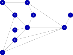
Figure 3: Topology of the graph of the coupled system and the pinned node.

The ordinary differential equation (2) is numerically solved by the Euler method with a time step $0.001$ (sec) and the time duration of the numerical simulations is $[0,2]$(sec).

IV-A Continuous-time monitoring

First, we consider the updating rule (9). According to $c\lambda_{2}>\alpha$, where $\lambda_{2}(L)$ is the smallest eigenvalue of $L$, except the unique zero eigenvalue, the supremum of the term $\beta^{\prime}/(c\sqrt{\lambda_{m}})$ is estimated as follows:

$$\sup\frac{\beta^{\prime}}{c\sqrt{\lambda_{m}(L)}}=\frac{c\lambda_{2}(L)-\lambda_{\max}(A_{2}^{s})}{c\sqrt{\lambda_{m}(L)}}\to\frac{\lambda_{2}(L)}{\sqrt{\lambda_{m}(L)}}$$

as $~{}c\to\infty$, by picking $\alpha=c\lambda_{2}(L)$. Fig. 4 shows the variation of $\beta^{\prime}/(c\sqrt{\lambda_{m}(L)})$ with respect to $c$. In this example, we pick $c=20.3281$, which implies $\beta^{\prime}/(c\sqrt{\lambda_{m}(L)})=0.1450$. We employ the updating rule (9) in Theorem 1. Fig. 5 presents the dynamics of each component of the $10$ nodes and show that the coupled system (2) reaches synchronization. Fig. 9 shows that $V(t)$ decreases with respect to time and converges toward zero as time goes to infinity.

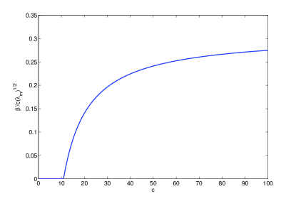
Figure 4: Variation of $\beta^{\prime}/(c\sqrt{\lambda_{m}})$ under continuous-time monitoring for synchronization with respect to the coupling strength $c$.

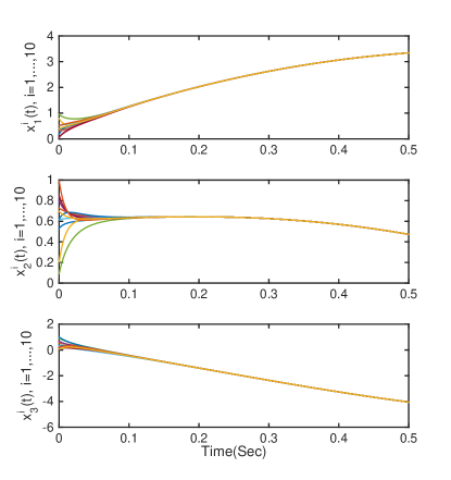
Figure 5: Dynamics of components of the coupled system (2) under the event triggering rule (9).

Second, we employ the updating rule (10). We take the same value of $c$ as above and $a=0.5$, $b=0.5$. Fig. 6 presents the dynamics of each component of the $10$ nodes and show that the coupled system (2) reaches synchronization. Fig. 9 shows that $V(t)$ decreases with time and converges to zero as time goes to infinity.

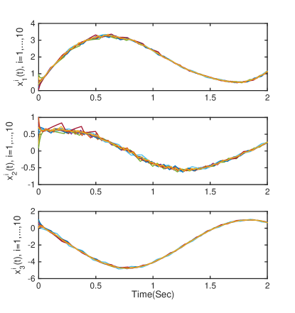
Figure 6: Dynamics of components of the coupled system (2) under the event triggering rule (10).

IV-B Discrete-time monitoring

First, we employ the updating rule (30). The term $\beta^{\prime}/(c\sqrt{\lambda_{m}})$ can be directly derived from the arguments above. We pick the same $c$ and then $\beta^{\prime}/(c\sqrt{\lambda_{m}})$ is the same as above. We employ the event trigger algorithm (30) in Theorem 3. Fig. 7 presents the dynamics of each component of the $10$ nodes and shows that the coupled system (2) reaches synchronisation. Fig. 9 shows that $V(t)$ decreases with time and converges to zero.

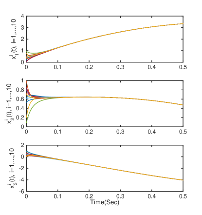
Figure 7: Dynamics of components of the coupled system (2) under the event triggering rule (30).

Second, we consider the updating rule (4). We pick the same $c$ as above and $a=0.5$, $b=0.5$. Fig. 8 presents the dynamics of each component of the $10$ nodes and show that the coupled system (2) reach synchronization. Fig. 9 shows that $V(t)$ decreases with respect to time and converges toward zero as time goes to infinity.

IV-C Performance comparison

In comparison, we consider the original linear coupled system as follows:

$$\frac{dx^{i}(t)}{dt}=f(x^{i}(t))-c\sum_{i=1}^{m}L_{ij}\Gamma(x^{j}(t)-x^{i}(t)),$$ (37)

for $i=1,\cdots,m$. By the same setups of model and numerical approach as above, its performance in terms of converge rates of $V(t)$ is shown similar with those of event-triggered rules (9) and (30), as comparatively shown by Fig. 9. As for the performance of rules (10) and (4), since the exponential convergence rates are pre-designed, as shown by (10) and (4), it is not surprising that their convergence rates are not as good as (37). However, their updating times of these rules are much less than those of rules (9) and (30), as comparatively shown in Figs. 10(a)-10(b).

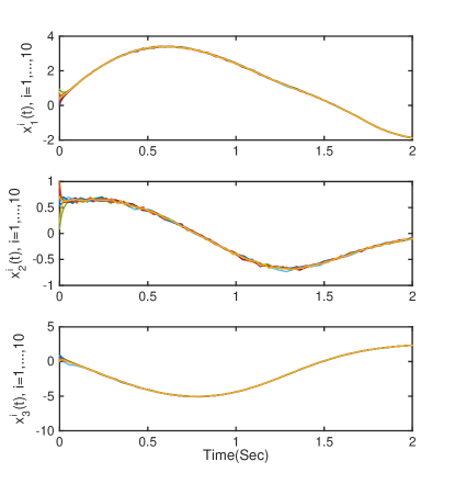
Figure 8: Dynamics of components of the coupled system (2) under the event triggering rule (4).

Figure 9: Dynamics of $V(t)$ for systems with continuous updating, continuous monitoring under rules (9),(10), discrete monitoring under rules (30), (4).

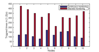
(a) under updating rules (9) and (30)

(b) under updating rules (10) and (4)

Figure 10: Histogram of triggering times of each node in $[1,2]$(sec).

V conclusion

In this paper, we employed event-triggered coupling configurations to realize synchronization for linearly coupled dynamical systems. We studied both continuous monitoring and discrete monitoring schemes: continuous monitoring scheme means that each node collects its neighborhood’s instantaneous state, and discrete monitoring scheme means that each node obtains its neighborhood’s states at the event triggered time. The event-triggered rules were proved to perform well and can exclude Zeno behaviors, as proved for some cases and illustrated by simulations. We showed that there are trade-offs between better performance in terms of fast convergence and less updating time slots, and between more cost in observation of states and more computation load of predicting next updating times. One step further, there are a few issues, including how to estimate the number of updating time slots and its dependence on the parameters in the rule and the structure of network structure, which merits the future research.

References

- [1] C. W. Wu and L. O. Chua, ”Synchronization in an array of linearly coupled dynamical systems,” IEEE Trans. Circuits Syst. I: Fundam. Theory Appl., vol. 42, pp. 430-447, Aug. 1995.
- [2] V. N. Belykh, I. V. Belykh, and M. Hasler, ”Connection graph stability method for synchronized coupled chaotic systems,” Physica D: Nonlinear Phenomena, vol. 195, no. 1, pp. 159-187, 2004.
- [3] W. Lu, T. Chen, ”Synchronization of coupled connected neural networks with delays,” IEEE Trans. Circuits Syst. I, Reg. Papers, vol. 51, pp. 2491-2503, Dec. 2004.
- [4] J. Cao, P. Li, and W. Wang, ”Global synchronization in arrays of delayed neural networks with constant and delayed coupling,” Phys. Lett. A, vol. 353, no. 4, pp. 318-325, 2006.
- [5] W. Lu and T. Chen, ”New approach to synchronization analysis of linearly coupled ordinary differential equations,” Physica D: Nonlinear Phenomena, vol. 213, no. 2, pp. 214-230, 2006.
- [6] J. Xiang and G. Chen, ”On the V-stability of complex dynamical networks,” Automatica, vol. 43, no. 6, pp. 1049-1057, 2007.
- [7] R. Olfati-Saber and R. M. Murray, ”Consensus problems in networks of agents with switching topology and time-delays,” IEEE Trans. Automat. Contr., vol. 49, pp. 1520-1533, Sep. 2004.
- [8] H. Zhang, J. Zhang, G.-H. Yang, and Y. Luo, ”Leader-based optimal coordination control for the consensus problem of multi-agent differential games via fuzzy adaptive dynamic programming,” IEEE Trans. Fuzzy Syst., vol. 23, pp. 152-163, Feb. 2015.
- [9] H. Zhang, T. Feng, G.-H. Yang, and H. Liang, ”Distributed cooperative optimal control for multiagent systems on directed graphs: an inverse optimal approach,” IEEE Trans. Cybern., to be published. DOI:10.1109/TCYB.2014.2350511
- [10] K. J. Åström and B. M. Bernhardsson, ”Comparison of Riemann and Lebesgue sampling for first order stochastic systems,” in Proceedings of the 41st IEEE Conference on Decision and Control, Las Vegas, Nevada USA, Dec. 2002, pp. 2011-2016.
- [11] M. Jr. Mazo and P. Tabuada, ”Decentralized event-triggered control over wireless sensor/actuator networks,” IEEE Trans. Automat. Contr., vol. 56, pp. 2456-2461, Aug. 2011.
- [12] X. Wang and M. D. Lemmon, ”Event-triggering in distributed networked control systems,” IEEE Trans. Automat. Contr., vol. 56, pp. 586-601, Mar. 2011.
- [13] D. V. Dimarogonas, E. Frazzoli, and K. H. Johansson, ”Distributed event-triggered control for multi-agent systems,” IEEE Trans. Automat. Contr., vol. 57, pp. 1291-1297, May 2012.
- [14] G. S. Seyboth, D. V. Dimarogonas, and K. H. Johansson, ”Event-based broadcasting for multi-agent average consensus,” Automatica, vol. 49, no. 1, pp. 245-252, 2013.
- [15] W. Lu and T. Chen, ”Synchronization analysis of linearly coupled networks of discrete time systems,” Physica D: Nonlinear Phenomena, vol.198, no. 1-2, pp. 148-168, 2004.
- [16] W. Lu and T. Chen, ”Global synchronization of discrete-time dynamical network with a directed graph,” IEEE Trans. Circuits Syst. II, Exp. Briefs, vol. 54, pp. 136-140, Feb. 2007.
- [17] P. Tabuada, ”Event-triggered real-time scheduling of stabilizing control tasks,” IEEE Trans. Automat. Contr., vol. 52, pp. 1680-1685, Sep. 2007.
- [18] H. Yu and P. J. Antsaklis, ”Output synchronization of multi-node systems with event-driven communication: communication delay and signal quantization”, Department of Electrical Engineering, University of Notre Dame, Jul. 2011, technical report.
- [19] H. Zhang, G. Feng, H. Yan, and Q. Chen, ”Observer-based output feedback event-triggered control for consensus of multi-agent systems,” IEEE Trans. Ind. Electron., vol. 61, pp. 4885-4894, Mar. 2014.
- [20] E. Johannesson, T. Henningsson, and A. Cervin, ”Sporadic control of first-order linear stochastic systems,” in 10th International Conference on Hybrid Systems: Computation and Control, Pisa, Italy, Apr. 2007, pp. 301-314.
- [21] M. Rabi, K. H. Johansson, and M. Johansson, ”Optimal stopping for event-triggered sensing and actuation”, in Proceedings of the 47th IEEE Conference on Decision and Control, Cancun, Mexico, Dec. 2008, pp. 3607-3612.
- [22] T. H. Gronwall, Note on the derivatives with respect to a parameter of the solutions of a system of differential equations, Ann. Math., vol. 20, no. 4, pp.292 -296, Jul. 1919.
- [23] R. Bellman, ”The stability of solutions of linear differential equations,” Duke Math. Jour., vol. 10, no. 4, pp. 643-647, 1943.
- [24] T. Matsumoto, L. O. Chua, and M. Komuro, ”The double scroll,” IEEE Trans. Circuits Syst., vol. 32, pp. 797-818, Aug. 1985.