\marginsize

1in1in0.5in1in

Spherical tϵsubscript𝑡italic-ϵt_{\epsilon}-Designs for Approximations on the Sphere

Yang Zhou Department of Applied Mathematics, The Hong Kong Polytechnic University. (Email: andres.zhou@connect.polyu.hk). This author’s work is supported in part by Hong Kong Research Council Grant PolyU5002/13p.    Xiaojun Chen Department of Applied Mathematics, The Hong Kong Polytechnic University (Email: maxjchen@polyu.edu.hk). This author’s work is supported in part by Hong Kong Research Council Grant PolyU5001/12p.
Abstract

A spherical t𝑡t-design is a set of points on the sphere that are nodes of a positive equal weight quadrature rule having algebraic accuracy t𝑡t for all spherical polynomials with degrees tabsent𝑡\leq t. Spherical t𝑡t-designs have many distinguished properties in approximations on the sphere and receive remarkable attention. Although the existence of a spherical t𝑡t-design is known for any t0𝑡0t\geq 0, a spherical design is only known in a set of interval enclosures on the sphere [15] for t100𝑡100t\leq 100. It is unknown how to choose a set of points from the set of interval enclosures to obtain a spherical t𝑡t-design. In this paper we investigate a new concept of point sets on the sphere named spherical tϵsubscript𝑡italic-ϵt_{\epsilon}-design (0<ϵ<10italic-ϵ10<\epsilon<1), which are nodes of a positive weight quadrature rule with algebraic accuracy t𝑡t. The sum of the weights is equal to the area of the sphere and the mean value of the weights is equal to the weight of the quadrature rule defined by the spherical t𝑡t-design. A spherical tϵsubscript𝑡italic-ϵt_{\epsilon}-design is a spherical t𝑡t-design when ϵ=0,italic-ϵ0\epsilon=0, and a spherical t𝑡t-design is a spherical tϵsubscript𝑡italic-ϵt_{\epsilon}-design for any 0<ϵ<10italic-ϵ10<\epsilon<1. We show that any point set chosen from the set of interval enclosures [15] is a spherical tϵsubscript𝑡italic-ϵt_{\epsilon}-design. We then study the worst-case errors of quadrature rules using spherical tϵsubscript𝑡italic-ϵt_{\epsilon}-designs in a Sobolev space, and investigate a model of polynomial approximation with the l1subscript𝑙1l_{1}-regularization using spherical tϵsubscript𝑡italic-ϵt_{\epsilon}-designs. Numerical results illustrate good performance of spherical tϵsubscript𝑡italic-ϵt_{\epsilon}-designs for numerical integration and function approximation on the sphere.

Keywords: spherical t𝑡t-designs, polynomial approximation, interval analysis, numerical integration, l1subscript𝑙1l_{1}-regularization

AMS suject classifications: 65D30, 41A10, 65G30

1 Introduction

For a d𝑑d-dimensional sphere

𝕊d:={𝐱=(x1,,xd+1)Td+1|𝐱22=1},assignsuperscript𝕊𝑑conditional-set𝐱superscriptsubscript𝑥1subscript𝑥𝑑1𝑇superscript𝑑1subscriptsuperscriptnorm𝐱221\mathbb{S}^{d}:=\{\mathbf{x}=(x_{1},\ldots,x_{d+1})^{T}\in\mathbb{R}^{d+1}\ |\ \|\mathbf{x}\|^{2}_{2}=1\},

where 2\|\cdot\|_{2} means the Euclidean norm, a spherical t𝑡t-design [17] for a given positive integer t𝑡t is a set of N𝑁N points XN={𝐱1,,𝐱N}𝕊dsubscript𝑋𝑁subscript𝐱1subscript𝐱𝑁superscript𝕊𝑑X_{N}=\{\mathbf{x}_{1},\ldots,\mathbf{x}_{N}\}\subset\mathbb{S}^{d} such that

1Nj=1Np(𝐱j)=1|𝕊d|𝕊dp(𝐱)dωd(𝐱)1𝑁superscriptsubscript𝑗1𝑁𝑝subscript𝐱𝑗1superscript𝕊𝑑subscriptsuperscript𝕊𝑑𝑝𝐱differential-dsubscript𝜔𝑑𝐱\frac{1}{N}\sum_{j=1}^{N}p(\mathbf{x}_{j})=\frac{1}{|\mathbb{S}^{d}|}\int_{\mathbb{S}^{d}}p(\mathbf{x}){\rm d}\omega_{d}(\mathbf{x}) (1)

holds for all spherical polynomials p𝑝p with degree tabsent𝑡\leq t, in which |𝕊d|superscript𝕊𝑑|\mathbb{S}^{d}| is the area of 𝕊dsuperscript𝕊𝑑\mathbb{S}^{d} and dωddsubscript𝜔𝑑{\rm d}\omega_{d} is the surface measure. For a numerical integration rule on the sphere, we say that the rule has algebraic accuracy t𝑡t, or the rule is of t𝑡t-algebraic accuracy, if the rule integrates all spherical polynomials with degree tabsent𝑡\leq t exactly. A spherical t𝑡t-design establishes a positive equal weight quadrature rule with algebraic accuracy t𝑡t for numerical integration on the whole sphere, which is also proved to perform well for numerical integration of spherical functions belonging to Sobolev spaces, see [12] for detail.

The existence of spherical t𝑡t-designs for arbitrary degree t𝑡t was proved by Seymour et al [26] in 1984. Consequently, a natural problem is to find the minimal number of points such that (1) holds for fixed t𝑡t and d𝑑d, denoted as N(d,t)𝑁𝑑𝑡N(d,t). In 1993, Korevaar et al [22] proved that N(d,t)Cdt(d2+d)/2𝑁𝑑𝑡subscript𝐶𝑑superscript𝑡superscript𝑑2𝑑2N(d,t)\leq C_{d}t^{(d^{2}+d)/2} and conjectured that N(d,t)Cdtd𝑁𝑑𝑡subscript𝐶𝑑superscript𝑡𝑑N(d,t)\leq C_{d}t^{d} for a sufficiently large positive constant Cdsubscript𝐶𝑑C_{d} depending only on d𝑑d. This conjecture was then proved by Bondarenko et al [10] in 2011. For d=2𝑑2d=2, there is an even stronger conjecture by Hardin et al [19] saying that N(2,t)12t2+o(t2)𝑁2𝑡12superscript𝑡2𝑜superscript𝑡2N(2,t)\leq\frac{1}{2}t^{2}+o(t^{2}) as t𝑡t\to\infty. Numerical evidence supporting the conjecture was also given in [19, 27]. Spherical t𝑡t-designs have been extensively studied from various viewpoints, among which the application to polynomial approximation and the number of points needed to construct a spherical t𝑡t-design have been paid great attention, see [2, 3, 5, 6, 7, 8, 15, 19, 22, 27]. Moreover, numerical methods have been developed for finding spherical t𝑡t-designs. Usually in those methods finding spherical designs is reformulated to problems of solving a system of nonlinear equations or optimization problems, see [2, 18, 27]. Numerical results suggest that those methods can find approximate spherical t𝑡t-designs with high precision.

However, in general, for any given t𝑡t the exact location of a spherical t𝑡t-design XN={𝐱1,,𝐱N}subscript𝑋𝑁subscript𝐱1subscript𝐱𝑁X_{N}=\{\mathbf{x}_{1},\ldots,\mathbf{x}_{N}\} is unknown. The best we know is that there is a set of points 𝐱^i,i=1,,Nformulae-sequencesubscript^𝐱𝑖𝑖1𝑁\hat{\mathbf{x}}_{i},\ i=1,\ldots,N such that a set of narrow intervals defined by

𝕏N={[𝐱]i=𝒞(𝐱^i,γi),i=1,,N,𝐱^i𝕊2,γi>0}𝕊2subscript𝕏𝑁formulae-sequencesubscriptdelimited-[]𝐱𝑖𝒞subscript^𝐱𝑖subscript𝛾𝑖formulae-sequence𝑖1𝑁formulae-sequencesubscript^𝐱𝑖superscript𝕊2subscript𝛾𝑖0superscript𝕊2\mathbb{X}_{N}=\{[\mathbf{x}]_{i}=\mathcal{C}(\hat{\mathbf{x}}_{i},\gamma_{i}),\ i=1,\ldots,N,\ \hat{\mathbf{x}}_{i}\in\mathbb{S}^{2},\ \gamma_{i}>0\}\subset\mathbb{S}^{2}

can be computed to contain a spherical t𝑡t-design for d=2𝑑2d=2, N=(t+1)2𝑁superscript𝑡12N=(t+1)^{2} and t100𝑡100t\leq 100 in [15], where

𝒞(𝐱^i,γi)={𝐱𝕊2cos1(𝐱𝐱^i)γi}.𝒞subscript^𝐱𝑖subscript𝛾𝑖conditional-set𝐱superscript𝕊2superscript1𝐱subscript^𝐱𝑖subscript𝛾𝑖\mathcal{C}(\hat{\mathbf{x}}_{i},\gamma_{i})=\{\mathbf{x}\in\mathbb{S}^{2}\mid\cos^{-1}(\mathbf{x}\cdot\hat{\mathbf{x}}_{i})\leq\gamma_{i}\}.

Among all the spherical polynomials with degree tabsent𝑡\leq t, if the zero polynomial is the only one that vanishes at each point in the set XN𝕊2subscript𝑋𝑁superscript𝕊2X_{N}\in\mathbb{S}^{2}, then the point set XN𝕊2subscript𝑋𝑁superscript𝕊2X_{N}\in\mathbb{S}^{2} is said to be fundamental with order t𝑡t. In 2011, Chen et al [15] proposed a computational-assisted proof for the existence of spherical t𝑡t-designs on 𝕊2superscript𝕊2\mathbb{S}^{2} with N=(t+1)2𝑁superscript𝑡12N=(t+1)^{2} for all values of t100𝑡100t\leq 100. An interval arithmetic based algorithm is proposed to compute a series of sets of polar coordinates type interval enclosures containing fundamental spherical t𝑡t-designs. By choosing the center points of each interval enclosures, an approximate spherical t𝑡t-design can be obtained and numerical results show that the Weyl sums of these point sets are very close to 0. However, though we have known the existence of spherical t𝑡t-designs for t100𝑡100t\leq 100 and N=(t+1)2𝑁superscript𝑡12N=(t+1)^{2} in a set of interval enclosures, we still can not obtain an exact spherical t𝑡t-design in the set of interval enclosures for a positive equal weight quadrature rule with algebraic accuracy t𝑡t. Motivated by this problem, in this paper we relax the equal weights to the ones whose mean value is still |𝕊d|Nsuperscript𝕊𝑑𝑁\frac{|\mathbb{S}^{d}|}{N} but can be chosen in an interval with respect to a number 0ϵ<10italic-ϵ10\leq\epsilon<1.

Definition 1.

(Spherical tϵsubscript𝑡italic-ϵt_{\epsilon}-deisgn) A spherical tϵsubscript𝑡italic-ϵt_{\epsilon}-design with 0ϵ<10italic-ϵ10\leq\epsilon<1 on 𝕊dsuperscript𝕊𝑑\mathbb{S}^{d} is a set of points XNϵ:={𝐱1ϵ,,𝐱Nϵ}𝕊dassignsubscriptsuperscript𝑋italic-ϵ𝑁superscriptsubscript𝐱1italic-ϵsuperscriptsubscript𝐱𝑁italic-ϵsuperscript𝕊𝑑X^{\epsilon}_{N}:=\{\mathbf{x}_{1}^{\epsilon},\ldots,\mathbf{x}_{N}^{\epsilon}\}\subset\mathbb{S}^{d} such that the quadrature rule with weights 𝐰=(w1,,wN)T𝐰superscriptsubscript𝑤1subscript𝑤𝑁𝑇\mathbf{w}=(w_{1},\ldots,w_{N})^{T} satisfying

|𝕊d|N(1ϵ)wi|𝕊d|N(1ϵ)1,i=1,,N,formulae-sequencesuperscript𝕊𝑑𝑁1italic-ϵsubscript𝑤𝑖superscript𝕊𝑑𝑁superscript1italic-ϵ1𝑖1𝑁\frac{|\mathbb{S}^{d}|}{N}(1-\epsilon)\leq w_{i}\leq\frac{|\mathbb{S}^{d}|}{N}(1-\epsilon)^{-1},\quad i=1,\ldots,N, (2)

is exact for all spherical polynomials p𝑝p of degree at most t𝑡t, that is,

i=1Nwip(𝐱iϵ)=𝕊dp(𝐱)dωd(𝐱).superscriptsubscript𝑖1𝑁subscript𝑤𝑖𝑝subscriptsuperscript𝐱italic-ϵ𝑖subscriptsuperscript𝕊𝑑𝑝𝐱differential-dsubscript𝜔𝑑𝐱\sum_{i=1}^{N}w_{i}p(\mathbf{x}^{\epsilon}_{i})=\int_{\mathbb{S}^{d}}p(\mathbf{x}){\rm d}\omega_{d}(\mathbf{x}). (3)

The concept of spherical tϵsubscript𝑡italic-ϵt_{\epsilon}-designs establishes a bridge of spherical t𝑡t-designs and ordinary positive weight quadrature rules with algebraic accuracy t𝑡t.

Remark 2.

A spherical t𝑡t-design is a spherical t0subscript𝑡0t_{0}-design with ϵ=0italic-ϵ0\epsilon=0. By letting p(𝐱)1𝑝𝐱1p(\mathbf{x})\equiv 1 in (3) we can obtain i=1Nwi=|𝕊d|superscriptsubscript𝑖1𝑁subscript𝑤𝑖superscript𝕊𝑑\sum_{i=1}^{N}w_{i}=|\mathbb{S}^{d}| and thus 0<wi<|𝕊d|0subscript𝑤𝑖superscript𝕊𝑑0<w_{i}<|\mathbb{S}^{d}| for i=1,,N𝑖1𝑁i=1,\ldots,N.

Since the existence of spherical t𝑡t-designs has been proved for arbitrary t𝑡t, and a spherical t𝑡t-design is also a spherical tϵsubscript𝑡italic-ϵt_{\epsilon}-design for arbitrary 0ϵ<10italic-ϵ10\leq\epsilon<1, we have the existence of spherical tϵsubscript𝑡italic-ϵt_{\epsilon}-designs. Due to the relaxation of the weights 𝐰𝐰\mathbf{w}, an important advantage is that we can have a positive weight quadrature rule with algebraic accuracy t𝑡t. Moreover, our numerical experiments show that with the increase of ϵitalic-ϵ\epsilon we can get numerical integration with polynomial precision using fewer points than spherical t𝑡t-designs.

The rest of this paper is organized as the following. In Section 2, we discuss the relationship between spherical tϵsubscript𝑡italic-ϵt_{\epsilon}-designs and spherical t𝑡t-designs when they are fundamental systems with same number of points. Based on the results we study the sets of interval enclosures containing fundamental spherical t𝑡t-designs in Section 3. We prove that all point sets arbitrarily chosen in those sets of interval enclosures computed in [15] are spherical tϵsubscript𝑡italic-ϵt_{\epsilon}-designs. In Section 4, we analyze the worst-case errors of spherical tϵsubscript𝑡italic-ϵt_{\epsilon}-designs for numerical integration on the unit sphere 𝕊2superscript𝕊2\mathbb{S}^{2}. Numerical results show that compared with the equal weight quadrature rules using spherical t𝑡t-designs, the worst-case errors can be improved with relaxing the weights to define quadrature rules using spherical tϵsubscript𝑡italic-ϵt_{\epsilon}-designs. In Section 5, we investigate an l2l1subscript𝑙2subscript𝑙1l_{2}-l_{1} regularized weighted least squares model for polynomial approximation on the two-sphere using spherical tϵsubscript𝑡italic-ϵt_{\epsilon}-designs and present numerical results to demonstrate the efficiency of the l2l1subscript𝑙2subscript𝑙1l_{2}-l_{1} model.

In this paper we concentrate on the case d=2𝑑2d=2. Throughout the paper we assume that all the points in a point set on the unit sphere are distinct. The computation is implemented in Matlab 2012b and done on a Lenovo Thinkcenter PC equipped with Intel Core i7-3770 3.4G Hz CPU, 8 GB RAM running Windows 7.

2 Spherical tϵsubscript𝑡italic-ϵt_{\epsilon}-designs: neighborhood of spherical t𝑡t-designs

In this section we will study the relationship between spherical tϵsubscript𝑡italic-ϵt_{\epsilon}-designs and spherical t𝑡t-designs when they are both fundamental systems and have the same number of points. A spherical t𝑡t-design defines an equal weight quadrature rule with algebraic accuracy t𝑡t while a spherical tϵsubscript𝑡italic-ϵt_{\epsilon}-design defines a positive weight quadrature rule with algebraic accuracy t𝑡t. Based on these two properties, in this section we study a neighborhood of spherical t𝑡t-designs. Denote

t:=t(𝕊2)assignsubscript𝑡subscript𝑡superscript𝕊2\displaystyle\mathbb{P}_{t}:=\mathbb{P}_{t}(\mathbb{S}^{2}) =\displaystyle= {spherical  polynomials  of  degree t }spherical  polynomials  of  degree t \displaystyle\{\mbox{spherical \ polynomials \ of \ degree \ $\leq t$ }\}
=\displaystyle= span{Y,k:=0,,t,k=1,,2+1},spanconditional-setsubscript𝑌𝑘formulae-sequence0𝑡𝑘121\displaystyle\mathrm{span}\{Y_{\ell,k}:\ell=0,\ldots,t,k=1,\ldots,2\ell+1\},

as the space of all spherical polynomials with degree tabsent𝑡\leq t on the unit two-sphere 𝕊2superscript𝕊2\mathbb{S}^{2}. Here Y,ksubscript𝑌𝑘Y_{\ell,k} is a fixed 𝕃2subscript𝕃2\mathbb{L}_{2}-orthogonormal real spherical harmonic of degree \ell and order k𝑘k, which means

𝕊2Y,k(𝐱)Y,k(𝐱)dω(𝐱)=δ,δk,k,,=0,,t;k,k=1,,2+1,formulae-sequencesubscriptsuperscript𝕊2subscript𝑌𝑘𝐱subscript𝑌superscriptsuperscript𝑘𝐱differential-d𝜔𝐱subscript𝛿superscriptsubscript𝛿𝑘superscript𝑘formulae-sequencesuperscript0𝑡𝑘superscript𝑘121\int_{\mathbb{S}^{2}}Y_{\ell,k}(\mathbf{x})Y_{\ell^{\prime},k^{\prime}}(\mathbf{x}){\rm d}\omega(\mathbf{x})=\delta_{\ell,\ell^{\prime}}\delta_{k,k^{\prime}},\quad\ell,\ell^{\prime}=0,\ldots,t;\ k,k^{\prime}=1,\ldots,2\ell+1, (4)

where dω(𝐱)=dω2(𝐱)d𝜔𝐱dsubscript𝜔2𝐱{\rm d}\omega(\mathbf{x})={\rm d}\omega_{2}(\mathbf{x}), and δ,subscript𝛿superscript\delta_{\ell,\ell^{\prime}} is the Kronecker delta. It is well known that

dt:=dim(t)==0t(2+1)=(t+1)2.assignsubscript𝑑𝑡dimsubscript𝑡superscriptsubscript0𝑡21superscript𝑡12d_{t}:=\mathrm{dim}(\mathbb{P}_{t})=\sum_{\ell=0}^{t}(2\ell+1)=(t+1)^{2}. (5)

By the addition theorem we have

k=12+1Y,k(𝐱)Y,k(𝐲)=2+14πP(𝐱𝐲),superscriptsubscript𝑘121subscript𝑌𝑘𝐱subscript𝑌𝑘𝐲214𝜋subscript𝑃𝐱𝐲\sum_{k=1}^{2\ell+1}Y_{\ell,k}(\mathbf{x})Y_{\ell,k}(\mathbf{y})=\frac{2\ell+1}{4\pi}P_{\ell}(\mathbf{x}\cdot\mathbf{y}), (6)

which implies k=12+1Y,k2(𝐱)=2+14πsuperscriptsubscript𝑘121superscriptsubscript𝑌𝑘2𝐱214𝜋\sum_{k=1}^{2\ell+1}Y_{\ell,k}^{2}(\mathbf{x})=\frac{2\ell+1}{4\pi}, where P,0subscript𝑃0P_{\ell},\ \ell\geq 0 denotes the Legendre Polynomial and 𝐱𝐲𝐱𝐲\mathbf{x}\cdot\mathbf{y} denotes the Euclidean inner product. Hence we obtain

Y,kC(𝕊2)max𝐱𝕊2(k=12+1Y,k2(𝐱))12=2+14πfork=1,,2+1,0.\|Y_{\ell,k}\|_{C(\mathbb{S}^{2})}\leq\max_{\mathbf{x}\in\mathbb{S}^{2}}\left(\sum_{k=1}^{2\ell+1}Y_{\ell,k}^{2}(\mathbf{x})\right)^{\frac{1}{2}}=\sqrt{\frac{2\ell+1}{4\pi}}\quad{\rm for}\ k=1,\ldots,2\ell+1,\ \ell\geq 0. (7)

Indeed, a spherical coordinate form of real spherical harmonics can be represented as (see [1, 4])

Y,k(𝐱)={2N,kP+1k(cosθ)coskφ,k=1,,,N,kP0(cosθ),k=+1,2N,kPk1(cosθ)sinkφ,k=+2,,2+1,subscript𝑌𝑘𝐱cases2subscript𝑁𝑘superscriptsubscript𝑃1𝑘𝜃𝑘𝜑𝑘1missing-subexpressionmissing-subexpressionsubscript𝑁𝑘superscriptsubscript𝑃0𝜃𝑘1missing-subexpressionmissing-subexpression2subscript𝑁𝑘superscriptsubscript𝑃𝑘1𝜃𝑘𝜑𝑘221Y_{\ell,k}(\mathbf{x})=\left\{\begin{array}[]{ll}\sqrt{2}N_{\ell,k}P_{\ell}^{\ell+1-k}(\cos\theta)\cos k\varphi,&k=1,\ldots,\ell,\\ \\ N_{\ell,k}P_{\ell}^{0}(\cos\theta),&k=\ell+1,\\ \\ \sqrt{2}N_{\ell,k}P_{\ell}^{k-\ell-1}(\cos\theta)\sin k\varphi,&k=\ell+2,\ldots,2\ell+1,\\ \end{array}\right. (8)

with

𝐱=(sinθcosφsinθsinφcosθ),𝐱𝜃𝜑𝜃𝜑𝜃\mathbf{x}=\left(\begin{array}[]{c}\sin\theta\cos\varphi\\ \sin\theta\sin\varphi\\ \cos\theta\\ \end{array}\right),

where 0θπ0𝜃𝜋0\leq\theta\leq\pi, 0φ<2π0𝜑2𝜋0\leq\varphi<2\pi and N,ksubscript𝑁𝑘N_{\ell,k} are the normalization coefficients

N,k=2+14π(|k1|)!(+|k1|)!,k=1,,2+1.formulae-sequencesubscript𝑁𝑘214𝜋𝑘1𝑘1𝑘121N_{\ell,k}=\sqrt{\frac{2\ell+1}{4\pi}\frac{(\ell-|k-\ell-1|)!}{(\ell+|k-\ell-1|)!}},\quad k=1,\ldots,2\ell+1.

When taking k=+1𝑘1k=\ell+1 and θ=0𝜃0\theta=0 we can obtain Y,+1(𝐱)2+14πsubscript𝑌1𝐱214𝜋Y_{\ell,\ell+1}(\mathbf{x})\equiv\sqrt{\frac{2\ell+1}{4\pi}} with 𝐱=(0,0,1)T𝐱superscript001𝑇\mathbf{x}=(0,0,1)^{T}. Therefore, (7) is a sharp upper bound of Y,kC(𝕊2)subscriptnormsubscript𝑌𝑘𝐶superscript𝕊2\|Y_{\ell,k}\|_{C(\mathbb{S}^{2})}. With the fact that all spherical harmonics are a basis of tsubscript𝑡\mathbb{P}_{t} we have that a finite point set XN={𝐱1,,𝐱N}subscript𝑋𝑁subscript𝐱1subscript𝐱𝑁X_{N}=\{\mathbf{x}_{1},\ldots,\mathbf{x}_{N}\} is a spherical t𝑡t-design if and only if the Weyl sums

i=1NY,k(𝐱i)=0,k=1,,2+1,=1,,t,formulae-sequencesuperscriptsubscript𝑖1𝑁subscript𝑌𝑘subscript𝐱𝑖0formulae-sequence𝑘1211𝑡\sum_{i=1}^{N}Y_{\ell,k}(\mathbf{x}_{i})=0,\quad k=1,\ldots,2\ell+1,\ \ell=1,\ldots,t, (9)

hold, see [17, 27] for details. Let XN={𝐱1,,𝐱N}𝕊2subscript𝑋𝑁subscript𝐱1subscript𝐱𝑁superscript𝕊2X_{N}=\{\mathbf{x}_{1},\cdots,\mathbf{x}_{N}\}\subset\mathbb{S}^{2} and XN={𝐱1,,𝐱N}𝕊2superscriptsubscript𝑋𝑁superscriptsubscript𝐱1superscriptsubscript𝐱𝑁superscript𝕊2X_{N}^{\prime}=\{\mathbf{x}_{1}^{\prime},\cdots,\mathbf{x}_{N}^{\prime}\}\subset\mathbb{S}^{2} be two point sets on the sphere. To describe the relationship among points and point sets, we introduce the following definitions of distances.

  • 1.

    Define the geodesic distance between two points 𝐱i,𝐱j𝕊2subscript𝐱𝑖subscript𝐱𝑗superscript𝕊2\mathbf{x}_{i},\mathbf{x}_{j}\in\mathbb{S}^{2} as

    dist(𝐱i,𝐱j)=cos1(𝐱i𝐱j).distsubscript𝐱𝑖subscript𝐱𝑗superscript1subscript𝐱𝑖subscript𝐱𝑗{\rm dist}(\mathbf{x}_{i},\mathbf{x}_{j})=\cos^{-1}(\mathbf{x}_{i}\cdot\mathbf{x}_{j}).
  • 2.

    Define the separation distance of a point set XNsubscript𝑋𝑁X_{N} as

    ρ(XN)=minijcos1(𝐱i𝐱j),𝜌subscript𝑋𝑁subscript𝑖𝑗superscript1subscript𝐱𝑖subscript𝐱𝑗\rho(X_{N})=\min_{i\neq j}\cos^{-1}(\mathbf{x}_{i}\cdot\mathbf{x}_{j}),

    which represents the minimal geodesic distance between two different points in XNsubscript𝑋𝑁X_{N}.

  • 3.

    Define the least distance from a point 𝐱𝕊2𝐱superscript𝕊2\mathbf{x}\in\mathbb{S}^{2} to a point set XNsubscript𝑋𝑁X_{N} as

    dist(𝐱,XN)=minidist(𝐱,𝐱i)=minicos1(𝐱𝐱i),dist𝐱subscript𝑋𝑁subscript𝑖dist𝐱subscript𝐱𝑖subscript𝑖superscript1𝐱subscript𝐱𝑖{\rm dist}(\mathbf{x},X_{N})=\min_{i}\ {\rm dist}(\mathbf{x},\mathbf{x}_{i})=\min_{i}\ \cos^{-1}(\mathbf{x}\cdot\mathbf{x}_{i}),

    which can be seen as the geodesic distance from 𝐱𝐱\mathbf{x} to its projection on XNsubscript𝑋𝑁X_{N}.

  • 4.

    Define the Hausdorff distance between two point sets XNsubscript𝑋𝑁X_{N} and XNsuperscriptsubscript𝑋𝑁X_{N}^{\prime} by

    σ(XN,XN)𝜎subscript𝑋𝑁superscriptsubscript𝑋𝑁\displaystyle\sigma(X_{N},X_{N}^{\prime}) =\displaystyle= max{maxidist(𝐱i,XN),maxidist(𝐱i,XN)}subscript𝑖distsuperscriptsubscript𝐱𝑖subscript𝑋𝑁subscript𝑖distsubscript𝐱𝑖superscriptsubscript𝑋𝑁\displaystyle\max\{\max_{i}{\rm dist}(\mathbf{x}_{i}^{\prime},X_{N}),\ \max_{i}{\rm dist}(\mathbf{x}_{i},X_{N}^{\prime})\} (10)
    =\displaystyle= max{maximinjcos1(𝐱i𝐱j),maxjminicos1(𝐱i𝐱j)}.subscript𝑖subscript𝑗superscript1superscriptsubscript𝐱𝑖subscript𝐱𝑗subscript𝑗subscript𝑖superscript1superscriptsubscript𝐱𝑖subscript𝐱𝑗\displaystyle\max\{\max_{i}\min_{j}\cos^{-1}(\mathbf{x}_{i}^{\prime}\cdot\mathbf{x}_{j}),\max_{j}\min_{i}\cos^{-1}(\mathbf{x}_{i}^{\prime}\cdot\mathbf{x}_{j})\}.

Note that σ(XN,XN)=σ(XN,XN)𝜎subscript𝑋𝑁superscriptsubscript𝑋𝑁𝜎superscriptsubscript𝑋𝑁subscript𝑋𝑁\sigma(X_{N},X_{N}^{\prime})=\sigma(X_{N}^{\prime},X_{N}) and σ(XN,XN)=0𝜎subscript𝑋𝑁superscriptsubscript𝑋𝑁0\sigma(X_{N},X_{N}^{\prime})=0 if and only if XN=XNsubscript𝑋𝑁superscriptsubscript𝑋𝑁X_{N}=X_{N}^{\prime}.

Remark 3.

For two point sets XNsubscript𝑋𝑁X_{N} and XNsuperscriptsubscript𝑋𝑁X_{N}^{\prime}, if σ(XN,XN)<12ρ(XN)𝜎subscript𝑋𝑁superscriptsubscript𝑋𝑁12𝜌subscript𝑋𝑁\sigma(X_{N},X_{N}^{\prime})<\frac{1}{2}\rho(X_{N}), then for each 𝐱iXNsubscript𝐱𝑖subscript𝑋𝑁\mathbf{x}_{i}\in X_{N} there exists a unique 𝐱jXN𝒞(𝐱i,12ρ(XN))superscriptsubscript𝐱𝑗superscriptsubscript𝑋𝑁𝒞subscript𝐱𝑖12𝜌subscript𝑋𝑁\mathbf{x}_{j}^{\prime}\in X_{N}^{\prime}\cap\mathcal{C}(\mathbf{x}_{i},\frac{1}{2}\rho(X_{N})), where

𝒞(𝐱i,12ρ(XN))={𝐱𝕊2cos1(𝐱𝐱i)12ρ(XN)}.𝒞subscript𝐱𝑖12𝜌subscript𝑋𝑁conditional-set𝐱superscript𝕊2superscript1𝐱subscript𝐱𝑖12𝜌subscript𝑋𝑁\mathcal{C}(\mathbf{x}_{i},\frac{1}{2}\rho(X_{N}))=\{\mathbf{x}\in\mathbb{S}^{2}\mid\cos^{-1}(\mathbf{x}\cdot\mathbf{x}_{i})\leq\frac{1}{2}\rho(X_{N})\}.

On account of the relationship between 𝒞(𝐱i,12ρ(XN))𝒞subscript𝐱𝑖12𝜌subscript𝑋𝑁\mathcal{C}(\mathbf{x}_{i},\frac{1}{2}\rho(X_{N})) and XNsuperscriptsubscript𝑋𝑁X_{N}^{\prime}, in what follows we will denote 𝐱isuperscriptsubscript𝐱𝑖\mathbf{x}_{i}^{\prime} as the point belonging to 𝒞(𝐱i,12ρ(XN))𝒞subscript𝐱𝑖12𝜌subscript𝑋𝑁\mathcal{C}(\mathbf{x}_{i},\frac{1}{2}\rho(X_{N})) for sake of consistency under the assumption σ(XN,XN)<12ρ(XN)𝜎subscript𝑋𝑁superscriptsubscript𝑋𝑁12𝜌subscript𝑋𝑁\sigma(X_{N},X_{N}^{\prime})<\frac{1}{2}\rho(X_{N}).

For a point set XN={𝐱1,,𝐱N}𝕊2subscript𝑋𝑁subscript𝐱1subscript𝐱𝑁superscript𝕊2X_{N}=\{\mathbf{x}_{1},\cdots,\mathbf{x}_{N}\}\subset\mathbb{S}^{2} we define the matrix 𝐘(XN)N×dt𝐘subscript𝑋𝑁superscript𝑁subscript𝑑𝑡\mathbf{Y}(X_{N})\in\mathbb{R}^{N\times d_{t}} with its elements as

𝐘i,2+k(XN)=Y,k(xi),i=1,,N,k=1,,2+1,=0,,t.formulae-sequencesubscript𝐘𝑖superscript2𝑘subscript𝑋𝑁subscript𝑌𝑘subscriptx𝑖formulae-sequence𝑖1𝑁formulae-sequence𝑘1210𝑡\mathbf{Y}_{i,\ell^{2}+k}(X_{N})=Y_{\ell,k}(\textbf{x}_{i}),\quad i=1,\ldots,N,\ k=1,\ldots,2\ell+1,\ \ell=0,\ldots,t. (11)

Note that |𝕊2|=4πsuperscript𝕊24𝜋|\mathbb{S}^{2}|=4\pi. An equivalent condition of spherical tϵsubscript𝑡italic-ϵt_{\epsilon}-designs given in [14] states that a point set XNϵ:={𝐱1ϵ,,𝐱Nϵ}𝕊2assignsubscriptsuperscript𝑋italic-ϵ𝑁subscriptsuperscript𝐱italic-ϵ1subscriptsuperscript𝐱italic-ϵ𝑁superscript𝕊2X^{\epsilon}_{N}:=\{\mathbf{x}^{\epsilon}_{1},\ldots,\mathbf{x}^{\epsilon}_{N}\}\subset\mathbb{S}^{2} is a spherical tϵsubscript𝑡italic-ϵt_{\epsilon}-design if and only if

𝐘(XNϵ)T𝐰4π𝐞1=𝟎and4π(1ϵ)N𝐞𝐰4π(1ϵ)1N𝐞,formulae-sequence𝐘superscriptsubscriptsuperscript𝑋italic-ϵ𝑁𝑇𝐰4𝜋subscript𝐞10and4𝜋1italic-ϵ𝑁𝐞𝐰4𝜋superscript1italic-ϵ1𝑁𝐞\mathbf{Y}(X^{\epsilon}_{N})^{T}\mathbf{w}-\sqrt{4\pi}\mathbf{e}_{1}=\mathbf{0}~{}~{}~{}~{}{\rm and}\quad\frac{4\pi(1-\epsilon)}{N}\mathbf{e}\leq\mathbf{w}\leq\frac{4\pi(1-\epsilon)^{-1}}{N}\mathbf{e}, (12)

where 𝐞1=(1,0,,0)T(L+1)2subscript𝐞1superscript100𝑇superscriptsuperscript𝐿12\mathbf{e}_{1}=(1,0,\ldots,0)^{T}\in\mathbb{R}^{(L+1)^{2}} and 𝐞=(1,,1)TN𝐞superscript11𝑇superscript𝑁\mathbf{e}=(1,\ldots,1)^{T}\in\mathbb{R}^{N}.

For two matrices constructed by two near enough point sets on 𝕊2superscript𝕊2\mathbb{S}^{2} we have the following property.

Proposition 4.

For any two point sets XNsubscript𝑋𝑁X_{N}, XN𝕊2superscriptsubscript𝑋𝑁superscript𝕊2X_{N}^{\prime}\subset\mathbb{S}^{2} satisfying σ(XN,XN)<12ρ(XN)𝜎subscript𝑋𝑁superscriptsubscript𝑋𝑁12𝜌subscript𝑋𝑁\sigma(X_{N},X_{N}^{\prime})<\frac{1}{2}\rho(X_{N}) there always holds

(𝐘(XN)𝐘(XN))Tsubscriptnormsuperscript𝐘subscript𝑋𝑁𝐘superscriptsubscript𝑋𝑁𝑇\displaystyle\|(\mathbf{Y}(X_{N})-\mathbf{Y}(X_{N}^{\prime}))^{T}\|_{\infty} =\displaystyle= 𝐘(XN)𝐘(XN)1subscriptnorm𝐘subscript𝑋𝑁𝐘superscriptsubscript𝑋𝑁1\displaystyle\|\mathbf{Y}(X_{N})-\mathbf{Y}(X_{N}^{\prime})\|_{1} (13)
\displaystyle\leq N(t+1)2t+14πσ(XN,XN),𝑁𝑡12𝑡14𝜋𝜎subscript𝑋𝑁superscriptsubscript𝑋𝑁\displaystyle N(t+1)\sqrt{\frac{2t+1}{4\pi}}\sigma(X_{N},X_{N}^{\prime}),

where 𝐘(XN),𝐘(XN)N×dt𝐘subscript𝑋𝑁𝐘superscriptsubscript𝑋𝑁superscript𝑁subscript𝑑𝑡\mathbf{Y}(X_{N}),\mathbf{Y}(X_{N}^{\prime})\in\mathbb{R}^{N\times d_{t}} are matrices defined by (11) which depend on t𝑡t.

Proof.

For a point 𝐱iXNsubscript𝐱𝑖subscript𝑋𝑁\mathbf{x}_{i}\in X_{N}, by Remark 3 we let 𝐱isuperscriptsubscript𝐱𝑖\mathbf{x}_{i}^{\prime} be the unique point located in 𝒞(𝐱i,12ρ(XN))XN𝒞subscript𝐱𝑖12𝜌subscript𝑋𝑁superscriptsubscript𝑋𝑁\mathcal{C}(\mathbf{x}_{i},\frac{1}{2}\rho(X_{N}))\cap X_{N}^{\prime}. Let Q,ksubscript𝑄𝑘Q_{\ell,k} be the restriction of Y,ksubscript𝑌𝑘Y_{\ell,k} on the great circle through these two points. Then Q,ksubscript𝑄𝑘Q_{\ell,k} is a trigonometric polynomial on the sphere and by Bernstein’s inequality [11] and (7) we obtain

|Y,k(𝐱i)Y,k(𝐱i)|subscript𝑌𝑘subscript𝐱𝑖subscript𝑌𝑘superscriptsubscript𝐱𝑖\displaystyle|Y_{\ell,k}(\mathbf{x}_{i})-Y_{\ell,k}(\mathbf{x}_{i}^{\prime})| =\displaystyle= |Q,k(𝐱i)Q,k(𝐱i)|subscript𝑄𝑘subscript𝐱𝑖subscript𝑄𝑘superscriptsubscript𝐱𝑖\displaystyle|Q_{\ell,k}(\mathbf{x}_{i})-Q_{\ell,k}(\mathbf{x}_{i}^{\prime})| (14)
\displaystyle\leq cos1(𝐱i𝐱i)sup|Q,k|superscript1subscript𝐱𝑖superscriptsubscript𝐱𝑖supremumsuperscriptsubscript𝑄𝑘\displaystyle\cos^{-1}(\mathbf{x}_{i}\cdot\mathbf{x}_{i}^{\prime})\sup|Q_{\ell,k}^{\prime}|
\displaystyle\leq cos1(𝐱i𝐱i)(t+1)sup|Q,k|superscript1subscript𝐱𝑖superscriptsubscript𝐱𝑖𝑡1supremumsubscript𝑄𝑘\displaystyle\cos^{-1}(\mathbf{x}_{i}\cdot\mathbf{x}_{i}^{\prime})(t+1)\sup|Q_{\ell,k}|
\displaystyle\leq cos1(𝐱i𝐱i)(t+1)Y,kC(𝕊2)superscript1subscript𝐱𝑖superscriptsubscript𝐱𝑖𝑡1subscriptnormsubscript𝑌𝑘𝐶superscript𝕊2\displaystyle\cos^{-1}(\mathbf{x}_{i}\cdot\mathbf{x}_{i}^{\prime})(t+1)\|Y_{\ell,k}\|_{C(\mathbb{S}^{2})}
\displaystyle\leq σ(XN,XN)(t+1)2+14π,𝜎subscript𝑋𝑁superscriptsubscript𝑋𝑁𝑡1214𝜋\displaystyle\sigma(X_{N},X_{N}^{\prime})(t+1)\sqrt{\frac{2\ell+1}{4\pi}},

where the last inequality is obtained by (7). Together with (13) and (14) we have

𝐘(XN)𝐘(XN)1subscriptnorm𝐘subscript𝑋𝑁𝐘superscriptsubscript𝑋𝑁1\displaystyle\|\mathbf{Y}(X_{N})-\mathbf{Y}(X_{N}^{\prime})\|_{1} =\displaystyle= max0t,1k2+1j=1N|Y,k(𝐱j)Y,k(𝐱j)|subscriptformulae-sequence0𝑡1𝑘21superscriptsubscript𝑗1𝑁subscript𝑌𝑘subscript𝐱𝑗subscript𝑌𝑘superscriptsubscript𝐱𝑗\displaystyle\max_{0\leq\ell\leq t,1\leq k\leq 2\ell+1}\sum_{j=1}^{N}|Y_{\ell,k}(\mathbf{x}_{j})-Y_{\ell,k}(\mathbf{x}_{j}^{\prime})|
\displaystyle\leq N(t+1)2t+14πσ(XN,XN).𝑁𝑡12𝑡14𝜋𝜎subscript𝑋𝑁superscriptsubscript𝑋𝑁\displaystyle N(t+1)\sqrt{\frac{2t+1}{4\pi}}\sigma(X_{N},X_{N}^{\prime}).

Let XN0={𝐱10,,𝐱N0}𝕊2superscriptsubscript𝑋𝑁0superscriptsubscript𝐱10superscriptsubscript𝐱𝑁0superscript𝕊2X_{N}^{0}=\{\mathbf{x}_{1}^{0},\ldots,\mathbf{x}_{N}^{0}\}\subset\mathbb{S}^{2} be a fundamental spherical t𝑡t-design. Given a number σ0superscript𝜎0\sigma^{\ast}\geq 0, denote the neighborhood of XN0superscriptsubscript𝑋𝑁0X_{N}^{0} with radius σsuperscript𝜎\sigma^{\ast} by

𝒞(XN0,σ)={XN𝕊2:σ(XN,XN0)σ}.𝒞superscriptsubscript𝑋𝑁0superscript𝜎conditional-setsubscript𝑋𝑁superscript𝕊2𝜎subscript𝑋𝑁superscriptsubscript𝑋𝑁0superscript𝜎\mathcal{C}(X_{N}^{0},\sigma^{\ast})=\big{\{}X_{N}\subset\mathbb{S}^{2}:\sigma(X_{N},X_{N}^{0})\leq\sigma^{\ast}\big{\}}.

The following lemma indicates that any point set contained in a small enough neighborhood of a fundamental spherical t𝑡t-design is a fundamental spherical tϵsubscript𝑡italic-ϵt_{\epsilon}-design.

Lemma 5.

Let XN0superscriptsubscript𝑋𝑁0X_{N}^{0} be a fundamental spherical t𝑡t-design with order t𝑡t and N=(t+1)2𝑁superscript𝑡12N=(t+1)^{2}. Then any point set XN𝒞(XN0,σ)subscript𝑋𝑁𝒞superscriptsubscript𝑋𝑁0superscript𝜎X_{N}\in\mathcal{C}(X_{N}^{0},\sigma^{\ast}) is a fundamental spherical tϵsubscript𝑡italic-ϵt_{\epsilon}-design with

τσ𝐘(XN0)111τσ𝐘(XN0)11ϵ<1,𝜏superscript𝜎subscriptnorm𝐘superscriptsuperscriptsubscript𝑋𝑁0111𝜏superscript𝜎subscriptnorm𝐘superscriptsuperscriptsubscript𝑋𝑁011italic-ϵ1\frac{\tau\sigma^{\ast}\|\mathbf{Y}(X_{N}^{0})^{-1}\|_{1}}{1-\tau\sigma^{\ast}\|\mathbf{Y}(X_{N}^{0})^{-1}\|_{1}}\leq\epsilon<1, (15)

where

σ<12min(1τ𝐘(XN0)11,ρ(XN0)),superscript𝜎121𝜏subscriptnorm𝐘superscriptsuperscriptsubscript𝑋𝑁011𝜌superscriptsubscript𝑋𝑁0\sigma^{\ast}<\frac{1}{2}\min\left(\frac{1}{\tau\|\mathbf{Y}(X_{N}^{0})^{-1}\|_{1}},\rho(X_{N}^{0})\right), (16)

with τ=2t+14π(t+1)3𝜏2𝑡14𝜋superscript𝑡13\tau=\sqrt{\frac{2t+1}{4\pi}}(t+1)^{3}.

Proof.

This lemma can be proved by showing that for any point set XN𝒞(XN0,σ)subscript𝑋𝑁𝒞superscriptsubscript𝑋𝑁0superscript𝜎X_{N}\in\mathcal{C}(X_{N}^{0},\sigma^{\ast}) we have

𝐘(XN)T𝐰=4π𝐞1,𝐘superscriptsubscript𝑋𝑁𝑇𝐰4𝜋subscript𝐞1\mathbf{Y}(X_{N})^{T}\mathbf{w}=\sqrt{4\pi}\mathbf{e}_{1}, (17)

in which 𝐘(XN)𝐘subscript𝑋𝑁\mathbf{Y}(X_{N}) is nonsingular and 𝐰4πN𝐞<4πNsubscriptnorm𝐰4𝜋𝑁𝐞4𝜋𝑁\|\mathbf{w}-\frac{4\pi}{N}\mathbf{e}\|_{\infty}<\frac{4\pi}{N}.

From Proposition 4 for any point set XNsubscript𝑋𝑁X_{N} with σ(XN,XN0)<σ𝜎subscript𝑋𝑁superscriptsubscript𝑋𝑁0superscript𝜎\sigma(X_{N},X_{N}^{0})<\sigma^{\ast} we have

𝐘(XN0)11𝐘(XN0)𝐘(XN)1<𝐘(XN0)11τσ<1.subscriptnorm𝐘superscriptsuperscriptsubscript𝑋𝑁011subscriptnorm𝐘superscriptsubscript𝑋𝑁0𝐘subscript𝑋𝑁1subscriptnorm𝐘superscriptsuperscriptsubscript𝑋𝑁011𝜏superscript𝜎1\|\mathbf{Y}(X_{N}^{0})^{-1}\|_{1}\|\mathbf{Y}(X_{N}^{0})-\mathbf{Y}(X_{N})\|_{1}<\|\mathbf{Y}(X_{N}^{0})^{-1}\|_{1}\tau\sigma^{\ast}<1.

Hence 𝐘(XN)𝐘subscript𝑋𝑁\mathbf{Y}(X_{N}) is nonsingular, that is, XNsubscript𝑋𝑁X_{N} is a fundamental system with order t𝑡t.

By the fact that XN0superscriptsubscript𝑋𝑁0X_{N}^{0} is a fundamental spherical t𝑡t-design and (9) we have

4πN𝐘(XN0)T𝐞=4π𝐞1.4𝜋𝑁𝐘superscriptsuperscriptsubscript𝑋𝑁0𝑇𝐞4𝜋subscript𝐞1\frac{4\pi}{N}\mathbf{Y}(X_{N}^{0})^{T}\mathbf{e}=\sqrt{4\pi}\mathbf{e}_{1}. (18)

Together with the well known perturbation theorem of linear systems in [30, Theorem 2.3.9, pp.135] and

𝐈𝐘(XN0))1𝐘(XN)T𝐘(XN0)11𝐘(XN0)𝐘(XN)1<1,\|\mathbf{I}-\mathbf{Y}(X_{N}^{0}))^{-1}\mathbf{Y}(X_{N})^{T}\|_{\infty}\leq\|\mathbf{Y}(X_{N}^{0})^{-1}\|_{1}\|\mathbf{Y}(X_{N}^{0})-\mathbf{Y}(X_{N})\|_{1}<1,

we have

𝐰4πN𝐞4πN𝐞(𝐘(XN0)T)1(𝐘(XN)𝐘(XN0))T1(𝐘(XN0)T)1(𝐘(XN)𝐘(XN0))T.subscriptnorm𝐰4𝜋𝑁𝐞subscriptnorm4𝜋𝑁𝐞subscriptnormsuperscript𝐘superscriptsuperscriptsubscript𝑋𝑁0𝑇1subscriptnormsuperscript𝐘subscript𝑋𝑁𝐘superscriptsubscript𝑋𝑁0𝑇1subscriptnormsuperscript𝐘superscriptsuperscriptsubscript𝑋𝑁0𝑇1subscriptnormsuperscript𝐘subscript𝑋𝑁𝐘superscriptsubscript𝑋𝑁0𝑇\frac{\|\mathbf{w}-\frac{4\pi}{N}\mathbf{e}\|_{\infty}}{\|\frac{4\pi}{N}\mathbf{e}\|_{\infty}}\leq\frac{\|(\mathbf{Y}(X_{N}^{0})^{T})^{-1}\|_{\infty}\ \|(\mathbf{Y}(X_{N})-\mathbf{Y}(X_{N}^{0}))^{T}\|_{\infty}}{1-\|(\mathbf{Y}(X_{N}^{0})^{T})^{-1}\|_{\infty}\|(\mathbf{Y}(X_{N})-\mathbf{Y}(X_{N}^{0}))^{T}\|_{\infty}}. (19)

Therefore, we obtain

𝐰4πN𝐞subscriptnorm𝐰4𝜋𝑁𝐞\displaystyle\|\mathbf{w}-\frac{4\pi}{N}\mathbf{e}\|_{\infty} =\displaystyle= 4πN𝐰4πN𝐞4πN𝐞4𝜋𝑁subscriptnorm𝐰4𝜋𝑁𝐞subscriptnorm4𝜋𝑁𝐞\displaystyle\frac{4\pi}{N}\frac{\|\mathbf{w}-\frac{4\pi}{N}\mathbf{e}\|_{\infty}}{\|\frac{4\pi}{N}\mathbf{e}\|_{\infty}}
\displaystyle\leq 4πN𝐘(XN0)11𝐘(XN0)𝐘(XN)11𝐘(XN0)𝐘(XN)1𝐘(XN0)114𝜋𝑁subscriptnorm𝐘superscriptsuperscriptsubscript𝑋𝑁011subscriptnorm𝐘superscriptsubscript𝑋𝑁0𝐘subscript𝑋𝑁11subscriptnorm𝐘superscriptsubscript𝑋𝑁0𝐘subscript𝑋𝑁1subscriptnorm𝐘superscriptsuperscriptsubscript𝑋𝑁011\displaystyle\frac{4\pi}{N}\frac{\|\mathbf{Y}(X_{N}^{0})^{-1}\|_{1}\|\mathbf{Y}(X_{N}^{0})-\mathbf{Y}(X_{N})\|_{1}}{1-\|\mathbf{Y}(X_{N}^{0})-\mathbf{Y}(X_{N})\|_{1}\|\mathbf{Y}(X_{N}^{0})^{-1}\|_{1}}
\displaystyle\leq 4πNτσ𝐘(XN0)111τσ𝐘(XN0)11<4πN.4𝜋𝑁𝜏superscript𝜎subscriptnorm𝐘superscriptsuperscriptsubscript𝑋𝑁0111𝜏superscript𝜎subscriptnorm𝐘superscriptsuperscriptsubscript𝑋𝑁0114𝜋𝑁\displaystyle\frac{4\pi}{N}\frac{\tau\sigma^{\ast}\|\mathbf{Y}(X_{N}^{0})^{-1}\|_{1}}{1-\tau\sigma^{\ast}\|\mathbf{Y}(X_{N}^{0})^{-1}\|_{1}}<\frac{4\pi}{N}.

Hence the vector 𝐰𝐰\mathbf{w} is positive which implies that XNsubscript𝑋𝑁X_{N} is spherical tϵsubscript𝑡italic-ϵt_{\epsilon}-design with ϵitalic-ϵ\epsilon satisfying (15). ∎

Based on above lemma we can deduce the following result which describes an upper bound of the radius of the neighborhood of a fundamental spherical t𝑡t-design, in which any point set located in the neighborhood is a fundamental spherical tϵsubscript𝑡italic-ϵt_{\epsilon}-design.

Corollary 6.

Let XN0superscriptsubscript𝑋𝑁0X_{N}^{0} be a fundamental spherical t𝑡t-design with order t𝑡t and N=(t+1)2𝑁superscript𝑡12N=(t+1)^{2}. For any 0ϵ<10italic-ϵ10\leq\epsilon<1, if

σ(XN,XN0)<min(12ρ(XN0),ϵτ(1+ϵ)𝐘(XN0)11),𝜎subscript𝑋𝑁superscriptsubscript𝑋𝑁012𝜌superscriptsubscript𝑋𝑁0italic-ϵ𝜏1italic-ϵsubscriptnorm𝐘superscriptsuperscriptsubscript𝑋𝑁011\sigma(X_{N},X_{N}^{0})<\min\left(\frac{1}{2}\rho(X_{N}^{0}),\frac{\epsilon}{\tau(1+\epsilon)\|\mathbf{Y}(X_{N}^{0})^{-1}\|_{1}}\right), (20)

then XNsubscript𝑋𝑁X_{N} is a fundamental spherical tϵsubscript𝑡italic-ϵt_{\epsilon}-design.

Proof.

By the fact that σ(XN,XN0)<σ𝜎subscript𝑋𝑁superscriptsubscript𝑋𝑁0superscript𝜎\sigma(X_{N},X_{N}^{0})<\sigma^{\ast} which is defined in (16), we have 𝐘(XN)𝐘subscript𝑋𝑁\mathbf{Y}(X_{N}) is nonsingular and

𝐰4πN𝐞4πNτσ(XN,XN0)𝐘(XN0)111τσ(XN,XN0)𝐘(XN0)11<4πNϵ.subscriptnorm𝐰4𝜋𝑁𝐞4𝜋𝑁𝜏𝜎subscript𝑋𝑁superscriptsubscript𝑋𝑁0subscriptnorm𝐘superscriptsuperscriptsubscript𝑋𝑁0111𝜏𝜎subscript𝑋𝑁superscriptsubscript𝑋𝑁0subscriptnorm𝐘superscriptsuperscriptsubscript𝑋𝑁0114𝜋𝑁italic-ϵ\displaystyle\|\mathbf{w}-\frac{4\pi}{N}\mathbf{e}\|_{\infty}\leq\frac{4\pi}{N}\frac{\tau\sigma(X_{N},X_{N}^{0})\|\mathbf{Y}(X_{N}^{0})^{-1}\|_{1}}{1-\tau\sigma(X_{N},X_{N}^{0})\|\mathbf{Y}(X_{N}^{0})^{-1}\|_{1}}<\frac{4\pi}{N}\epsilon.

Hence, from (20), we derive

(1ϵ)4πN𝐞<𝐰<(1+ϵ)4πN𝐞4π(1ϵ)1N𝐞.1italic-ϵ4𝜋𝑁𝐞𝐰1italic-ϵ4𝜋𝑁𝐞4𝜋superscript1italic-ϵ1𝑁𝐞(1-\epsilon)\frac{4\pi}{N}\mathbf{e}<\mathbf{w}<(1+{\epsilon})\frac{4\pi}{N}\mathbf{e}\leq\frac{4\pi(1-\epsilon)^{-1}}{N}\mathbf{e}.

We complete the proof. ∎

3 Interval analysis of spherical t𝑡t-designs and spherical tϵsubscript𝑡italic-ϵt_{\epsilon}-designs

In this section we will study the sets of interval enclosures containing fundamental spherical t𝑡t-designs. In the last section we describe a neighborhood of a fundamental spherical t𝑡t-design in which any point set is a fundamental spherical tϵsubscript𝑡italic-ϵt_{\epsilon}-design. A series of sets of interval enclosures of spherical t𝑡t-designs can be computed in [15], but the exact location of spherical t𝑡t-designs can not be obtained. In the following we will show that any point set in the set of the interval enclosures given in [15] is a fundamental spherical tϵsubscript𝑡italic-ϵt_{\epsilon}-design. Let

𝕏N={[𝐱]i=𝒞(𝐱^i,γi)𝕊2,i=1,,N}\mathbb{X}_{N}=\{[\mathbf{x}]_{i}=\mathcal{C}(\hat{\mathbf{x}}_{i},\gamma_{i})\subset\mathbb{S}^{2},\ i=1,\ldots,N\} (21)

be a set of spherical caps, with 𝐱^isubscript^𝐱𝑖\hat{\mathbf{x}}_{i} as the center point and γisubscript𝛾𝑖\gamma_{i} as the radius. Additionally, let X^N={𝐱^1,,𝐱^N}𝕊2subscript^𝑋𝑁subscript^𝐱1subscript^𝐱𝑁superscript𝕊2\hat{X}_{N}=\{\hat{\mathbf{x}}_{1},\ldots,\hat{\mathbf{x}}_{N}\}\subset\mathbb{S}^{2} be the set of center points. Define the radius of 𝕏Nsubscript𝕏𝑁\mathbb{X}_{N} by

rad(𝕏N)=max1iNγi,radsubscript𝕏𝑁subscript1𝑖𝑁subscript𝛾𝑖{\rm rad}(\mathbb{X}_{N})=\max_{1\leq i\leq N}\gamma_{i},

and the separation distance of 𝕏Nsubscript𝕏𝑁\mathbb{X}_{N} by

ρ(𝕏N)=minij𝐱i[𝐱]i,𝐱j[𝐱]j,dist(𝐱i,𝐱j).𝜌subscript𝕏𝑁subscript𝑖𝑗formulae-sequencesubscript𝐱𝑖subscriptdelimited-[]𝐱𝑖subscript𝐱𝑗subscriptdelimited-[]𝐱𝑗distsubscript𝐱𝑖subscript𝐱𝑗\rho(\mathbb{X}_{N})=\min_{\tiny{\begin{array}[]{c}i\neq j\\ \mathbf{x}_{i}\in[\mathbf{x}]_{i},\mathbf{x}_{j}\in[\mathbf{x}]_{j},\end{array}}}{\rm dist}(\mathbf{x}_{i},\mathbf{x}_{j}).

We say that 𝕏Nsubscript𝕏𝑁\mathbb{X}_{N} is an interval enclosure of a point set XN={𝐱1,,𝐱N}subscript𝑋𝑁subscript𝐱1subscript𝐱𝑁X_{N}=\{\mathbf{x}_{1},\ldots,\mathbf{x}_{N}\}, denoted as XN𝕏Nsubscript𝑋𝑁subscript𝕏𝑁X_{N}\in\mathbb{X}_{N}, if 𝐱i[𝐱]isubscript𝐱𝑖subscriptdelimited-[]𝐱𝑖\mathbf{x}_{i}\in[\mathbf{x}]_{i} and 𝐱i[𝐱]jsubscript𝐱𝑖subscriptdelimited-[]𝐱𝑗\mathbf{x}_{i}\notin[\mathbf{x}]_{j} for i=1,,N𝑖1𝑁i=1,\ldots,N and ij𝑖𝑗i\neq j.

Assumption 7.

Let 𝕏Nsubscript𝕏𝑁\mathbb{X}_{N} defined by (21) be a set of intervals. Assume that

  1. 1.

    there exists a spherical t𝑡t-design XN0𝕏Nsuperscriptsubscript𝑋𝑁0subscript𝕏𝑁X_{N}^{0}\in\mathbb{X}_{N};

  2. 2.

    𝐘(X^N)𝐘subscript^𝑋𝑁\mathbf{Y}(\hat{X}_{N}) is nonsingular.

The assumption that 𝐘(X^N)𝐘subscript^𝑋𝑁\mathbf{Y}(\hat{X}_{N}) is nonsingular also implies that 𝐘(X^N)𝐘subscript^𝑋𝑁\mathbf{Y}(\hat{X}_{N}) is a square matrix which requires N=(t+1)2𝑁superscript𝑡12N=(t+1)^{2}. In the following theorem we show that under Assumption 7 if rad(𝕏N)radsubscript𝕏𝑁{\rm rad}(\mathbb{X}_{N}) is smaller than a certain number, then 𝐘(XN)𝐘subscript𝑋𝑁\mathbf{Y}(X_{N}) is nonsingular and (20) holds for any XN𝕏Nsubscript𝑋𝑁subscript𝕏𝑁X_{N}\in\mathbb{X}_{N}.

Theorem 8.

Under Assumption 7, any point set XN𝕏Nsubscript𝑋𝑁subscript𝕏𝑁X_{N}\in\mathbb{X}_{N} is a fundamental spherical tϵsubscript𝑡italic-ϵt_{\epsilon}-design with

2τrad(𝕏N)𝐘(X^N)1114τrad(𝕏N)𝐘(X^N)11ϵ<1,2𝜏radsubscript𝕏𝑁subscriptnorm𝐘superscriptsubscript^𝑋𝑁1114𝜏radsubscript𝕏𝑁subscriptnorm𝐘superscriptsubscript^𝑋𝑁11italic-ϵ1\frac{2\tau{\rm rad}(\mathbb{X}_{N})\|\mathbf{Y}(\hat{X}_{N})^{-1}\|_{1}}{1-4\tau{\rm rad}(\mathbb{X}_{N})\|\mathbf{Y}(\hat{X}_{N})^{-1}\|_{1}}\leq\epsilon<1, (22)

if

rad(𝕏N)<min(14ρ(𝕏N),ϵ2(1+2ϵ)τ𝐘(X^N)11).radsubscript𝕏𝑁14𝜌subscript𝕏𝑁italic-ϵ212italic-ϵ𝜏subscriptnorm𝐘superscriptsubscript^𝑋𝑁11{\rm rad}(\mathbb{X}_{N})<\min\left(\frac{1}{4}\rho(\mathbb{X}_{N}),\dfrac{\epsilon}{2(1+2\epsilon)\tau\|\mathbf{Y}(\hat{X}_{N})^{-1}\|_{1}}\right). (23)
Proof.

For any XN𝕏Nsubscript𝑋𝑁subscript𝕏𝑁X_{N}\in\mathbb{X}_{N} it can be concluded that

ρ(XN)ρ(𝕏N).𝜌subscript𝑋𝑁𝜌subscript𝕏𝑁\rho(X_{N})\geq\rho(\mathbb{X}_{N}).

Hence for any two point sets XN,XN𝕏Nsubscript𝑋𝑁superscriptsubscript𝑋𝑁subscript𝕏𝑁X_{N},X_{N}^{\prime}\in\mathbb{X}_{N} we have

σ(XN,XN)max1iNmax𝐱i,𝐲i[𝐱]idist(𝐱i,𝐲i)=2rad(𝕏N).𝜎subscript𝑋𝑁superscriptsubscript𝑋𝑁subscript1𝑖𝑁subscriptsubscript𝐱𝑖subscript𝐲𝑖subscriptdelimited-[]𝐱𝑖distsubscript𝐱𝑖subscript𝐲𝑖2radsubscript𝕏𝑁\sigma(X_{N},X_{N}^{\prime})\leq\max_{1\leq i\leq N}\max_{\tiny{\mathbf{x}_{i},\mathbf{y}_{i}\in[\mathbf{x}]_{i}}}{\rm dist}(\mathbf{x}_{i},\mathbf{y}_{i})=2{\rm rad}(\mathbb{X}_{N}).

First we show that 𝐘(XN)𝐘subscript𝑋𝑁\mathbf{Y}(X_{N}) is nonsingular for any XN𝕏Nsubscript𝑋𝑁subscript𝕏𝑁X_{N}\in\mathbb{X}_{N}. By Proposition 4 we have

I𝐘(X^N)1𝐘(XN)1subscriptnormI𝐘superscriptsubscript^𝑋𝑁1𝐘subscript𝑋𝑁1\displaystyle\|{\rm I}-\mathbf{Y}(\hat{X}_{N})^{-1}\mathbf{Y}(X_{N})\|_{1} \displaystyle\leq 𝐘(X^N)11𝐘(X^N)𝐘(XN)1subscriptnorm𝐘superscriptsubscript^𝑋𝑁11subscriptnorm𝐘subscript^𝑋𝑁𝐘subscript𝑋𝑁1\displaystyle\|\mathbf{Y}(\hat{X}_{N})^{-1}\|_{1}\|\mathbf{Y}(\hat{X}_{N})-\mathbf{Y}(X_{N})\|_{1}
\displaystyle\leq 𝐘(X^N)11τσ(X^N,XN)subscriptnorm𝐘superscriptsubscript^𝑋𝑁11𝜏𝜎subscript^𝑋𝑁subscript𝑋𝑁\displaystyle\|\mathbf{Y}(\hat{X}_{N})^{-1}\|_{1}\tau\sigma(\hat{X}_{N},X_{N})
\displaystyle\leq 2τ𝐘(X^N)11rad(𝕏)<1.2𝜏subscriptnorm𝐘superscriptsubscript^𝑋𝑁11radsubscript𝕏1\displaystyle 2\tau\|\mathbf{Y}(\hat{X}_{N})^{-1}\|_{1}{\rm rad}(\mathbb{X_{N}})<1.

Hence all the point sets XN𝕏Nsubscript𝑋𝑁subscript𝕏𝑁X_{N}\in\mathbb{X}_{N} including XN0superscriptsubscript𝑋𝑁0X_{N}^{0} are fundamental systems with order t𝑡t. Moreover, from (23) we have

σ(XN,XN0)<12ρ(XN0).𝜎subscript𝑋𝑁superscriptsubscript𝑋𝑁012𝜌superscriptsubscript𝑋𝑁0\sigma(X_{N},X_{N}^{0})<\frac{1}{2}\rho(X_{N}^{0}).

By (23) we can also have

2(1+ϵ)τrad(𝕏N)𝐘(X^N)11<ϵ2ϵτrad(𝕏N)𝐘(X^N)11.evaluated-at21italic-ϵ𝜏radsubscript𝕏𝑁subscriptnorm𝐘superscriptsubscript^𝑋𝑁11braitalic-ϵ2italic-ϵ𝜏radsubscript𝕏𝑁𝐘superscriptsubscript^𝑋𝑁112(1+\epsilon)\tau{\rm rad}(\mathbb{X}_{N})\|\mathbf{Y}(\hat{X}_{N})^{-1}\|_{1}<\epsilon-2\epsilon\tau{\rm rad}(\mathbb{X}_{N})\|\mathbf{Y}(\hat{X}_{N})^{-1}\|_{1}.

By Corollary 2.7 in [29, pp.119] it can be concluded that for arbitrary XN𝕏Nsubscript𝑋𝑁subscript𝕏𝑁X_{N}\in\mathbb{X}_{N} we have

𝐘(XN)11𝐘(X^N)111𝐘(X^N)11𝐘(X^N)𝐘(XN)1.subscriptnorm𝐘superscriptsubscript𝑋𝑁11subscriptnorm𝐘superscriptsubscript^𝑋𝑁111subscriptnorm𝐘superscriptsubscript^𝑋𝑁11subscriptnorm𝐘subscript^𝑋𝑁𝐘subscript𝑋𝑁1\|\mathbf{Y}(X_{N})^{-1}\|_{1}\leq\dfrac{\|\mathbf{Y}(\hat{X}_{N})^{-1}\|_{1}}{1-\|\mathbf{Y}(\hat{X}_{N})^{-1}\|_{1}\|\mathbf{Y}(\hat{X}_{N})-\mathbf{Y}(X_{N})\|_{1}}. (24)

Then together with Proposition 4 we have

σ(XN,XN0)𝜎subscript𝑋𝑁superscriptsubscript𝑋𝑁0\displaystyle\sigma(X_{N},X_{N}^{0}) \displaystyle\leq 2rad(𝕏N)2radsubscript𝕏𝑁\displaystyle 2{\rm rad}(\mathbb{X}_{N}) (25)
<\displaystyle< ϵ(12τrad(𝕏N)𝐘(X^N)11)(1+ϵ)τ𝐘(X^N)11italic-ϵ12𝜏radsubscript𝕏𝑁subscriptnorm𝐘superscriptsubscript^𝑋𝑁111italic-ϵ𝜏subscriptnorm𝐘superscriptsubscript^𝑋𝑁11\displaystyle\frac{\epsilon(1-2\tau{\rm rad}(\mathbb{X}_{N})\|\mathbf{Y}(\hat{X}_{N})^{-1}\|_{1})}{(1+\epsilon)\tau\|\mathbf{Y}(\hat{X}_{N})^{-1}\|_{1}}
\displaystyle\leq ϵ(1𝐘(X^N)11𝐘(X^N)𝐘(XN0)1)(1+ϵ)τ𝐘(X^N)11italic-ϵ1subscriptnorm𝐘superscriptsubscript^𝑋𝑁11subscriptnorm𝐘subscript^𝑋𝑁𝐘superscriptsubscript𝑋𝑁011italic-ϵ𝜏subscriptnorm𝐘superscriptsubscript^𝑋𝑁11\displaystyle\frac{\epsilon(1-\|\mathbf{Y}(\hat{X}_{N})^{-1}\|_{1}\|\mathbf{Y}(\hat{X}_{N})-\mathbf{Y}(X_{N}^{0})\|_{1})}{(1+\epsilon)\tau\|\mathbf{Y}(\hat{X}_{N})^{-1}\|_{1}}
\displaystyle\leq ϵ(1+ϵ)τ𝐘(XN0)11.italic-ϵ1italic-ϵ𝜏subscriptnorm𝐘superscriptsuperscriptsubscript𝑋𝑁011\displaystyle\frac{\epsilon}{(1+\epsilon)\tau\|\mathbf{Y}(X_{N}^{0})^{-1}\|_{1}}.

By Corollary 6 we have that any point set XN𝕏Nsubscript𝑋𝑁subscript𝕏𝑁X_{N}\in\mathbb{X}_{N} is a fundamental spherical tϵsubscript𝑡italic-ϵt_{\epsilon}-design. Additionally, together with

𝐰4πN𝐞subscriptnorm𝐰4𝜋𝑁𝐞\displaystyle\|\mathbf{w}-\frac{4\pi}{N}\mathbf{e}\|_{\infty} \displaystyle\leq 4πN𝐘(XN0)11𝐘(XN0)𝐘(XN)11𝐘(XN0)𝐘(XN)1𝐘(XN0)114𝜋𝑁subscriptnorm𝐘superscriptsuperscriptsubscript𝑋𝑁011subscriptnorm𝐘superscriptsubscript𝑋𝑁0𝐘subscript𝑋𝑁11subscriptnorm𝐘superscriptsubscript𝑋𝑁0𝐘subscript𝑋𝑁1subscriptnorm𝐘superscriptsuperscriptsubscript𝑋𝑁011\displaystyle\frac{4\pi}{N}\frac{\|\mathbf{Y}(X_{N}^{0})^{-1}\|_{1}\|\mathbf{Y}(X_{N}^{0})-\mathbf{Y}(X_{N})\|_{1}}{1-\|\mathbf{Y}(X_{N}^{0})-\mathbf{Y}(X_{N})\|_{1}\|\mathbf{Y}(X_{N}^{0})^{-1}\|_{1}}
\displaystyle\leq 4πN2τrad(𝕏N)𝐘(XN0)1112τrad(𝕏N)𝐘(XN0)11,4𝜋𝑁2𝜏radsubscript𝕏𝑁subscriptnorm𝐘superscriptsuperscriptsubscript𝑋𝑁01112𝜏radsubscript𝕏𝑁subscriptnorm𝐘superscriptsuperscriptsubscript𝑋𝑁011\displaystyle\frac{4\pi}{N}\frac{2\tau{\rm rad}(\mathbb{X}_{N})\|\mathbf{Y}(X_{N}^{0})^{-1}\|_{1}}{1-2\tau{\rm rad}(\mathbb{X}_{N})\|\mathbf{Y}(X_{N}^{0})^{-1}\|_{1}},

and (24) we have

2τrad(𝕏N)𝐘(XN0)1112τrad(𝕏N)𝐘(XN0)112𝜏radsubscript𝕏𝑁subscriptnorm𝐘superscriptsuperscriptsubscript𝑋𝑁01112𝜏radsubscript𝕏𝑁subscriptnorm𝐘superscriptsuperscriptsubscript𝑋𝑁011\displaystyle\frac{2\tau{\rm rad}(\mathbb{X}_{N})\|\mathbf{Y}(X_{N}^{0})^{-1}\|_{1}}{1-2\tau{\rm rad}(\mathbb{X}_{N})\|\mathbf{Y}(X_{N}^{0})^{-1}\|_{1}}
\displaystyle\leq 2τrad(𝕏N)𝐘(X^N)111𝐘(X^N)11𝐘(X^N)𝐘(XN)112τrad(𝕏N)𝐘(X^N)111𝐘(X^N)11𝐘(X^N)𝐘(XN)12𝜏radsubscript𝕏𝑁subscriptnorm𝐘superscriptsubscript^𝑋𝑁111subscriptnorm𝐘superscriptsubscript^𝑋𝑁11subscriptnorm𝐘subscript^𝑋𝑁𝐘subscript𝑋𝑁112𝜏radsubscript𝕏𝑁subscriptnorm𝐘superscriptsubscript^𝑋𝑁111subscriptnorm𝐘superscriptsubscript^𝑋𝑁11subscriptnorm𝐘subscript^𝑋𝑁𝐘subscript𝑋𝑁1\displaystyle\frac{2\tau{\rm rad}(\mathbb{X}_{N})\dfrac{\|\mathbf{Y}(\hat{X}_{N})^{-1}\|_{1}}{1-\|\mathbf{Y}(\hat{X}_{N})^{-1}\|_{1}\|\mathbf{Y}(\hat{X}_{N})-\mathbf{Y}(X_{N})\|_{1}}}{1-2\tau{\rm rad}(\mathbb{X}_{N})\dfrac{\|\mathbf{Y}(\hat{X}_{N})^{-1}\|_{1}}{1-\|\mathbf{Y}(\hat{X}_{N})^{-1}\|_{1}\|\mathbf{Y}(\hat{X}_{N})-\mathbf{Y}(X_{N})\|_{1}}}
\displaystyle\leq 2τrad(𝕏N)𝐘(X^N)1114τrad(𝕏N)𝐘(X^N)11.2𝜏radsubscript𝕏𝑁subscriptnorm𝐘superscriptsubscript^𝑋𝑁1114𝜏radsubscript𝕏𝑁subscriptnorm𝐘superscriptsubscript^𝑋𝑁11\displaystyle\frac{2\tau{\rm rad}(\mathbb{X}_{N})\|\mathbf{Y}(\hat{X}_{N})^{-1}\|_{1}}{1-4\tau{\rm rad}(\mathbb{X}_{N})\|\mathbf{Y}(\hat{X}_{N})^{-1}\|_{1}}.

Then we have that any point set XN𝕏Nsubscript𝑋𝑁subscript𝕏𝑁X_{N}\in\mathbb{X}_{N} is a spherical tϵsubscript𝑡italic-ϵt_{\epsilon}-design with

2τrad(𝕏N)𝐘(X^N)1114τrad(𝕏N)𝐘(X^N)11ϵ<1,2𝜏radsubscript𝕏𝑁subscriptnorm𝐘superscriptsubscript^𝑋𝑁1114𝜏radsubscript𝕏𝑁subscriptnorm𝐘superscriptsubscript^𝑋𝑁11italic-ϵ1\frac{2\tau{\rm rad}(\mathbb{X}_{N})\|\mathbf{Y}(\hat{X}_{N})^{-1}\|_{1}}{1-4\tau{\rm rad}(\mathbb{X}_{N})\|\mathbf{Y}(\hat{X}_{N})^{-1}\|_{1}}\leq\epsilon<1,

under the assumption of rad(𝕏N)radsubscript𝕏𝑁{\rm rad}(\mathbb{X}_{N}). ∎

Theorem 8 proves that an arbitrarily chosen point set in a set of interval enclosures of a fundamental spherical t𝑡t-design is a spherical tϵsubscript𝑡italic-ϵt_{\epsilon}-design if rad(𝕏N)radsubscript𝕏𝑁{\rm rad}(\mathbb{X}_{N}) is smaller than a certain number. In the theorem we discuss the interval enclosures defined by spherical caps as [𝐱]i=𝒞(𝐱^i,γi)={𝐱𝕊2|cos1(𝐱𝐱^i)γi}subscriptdelimited-[]𝐱𝑖𝒞subscript^𝐱𝑖subscript𝛾𝑖conditional-set𝐱superscript𝕊2superscript1𝐱subscript^𝐱𝑖subscript𝛾𝑖[\mathbf{x}]_{i}=\mathcal{C}(\hat{\mathbf{x}}_{i},\gamma_{i})=\{\mathbf{x}\in\mathbb{S}^{2}|\cos^{-1}(\mathbf{x}\cdot\hat{\mathbf{x}}_{i})\leq\gamma_{i}\} for which many nice properties of real spherical harmonics can be adopted. However, in practice, to reduce the spherical constraint of points and the dimension of variables, the spherical coordinate form of the points are preferable to compute the interval enclosures, see [15]. For a point 𝐱iXN𝕊2subscript𝐱𝑖subscript𝑋𝑁superscript𝕊2\mathbf{x}_{i}\in X_{N}\subset\mathbb{S}^{2}, denote θisubscript𝜃𝑖\theta_{i}, φisubscript𝜑𝑖\varphi_{i} as its spherical coordinate. Then in [15] a series of intervals [θ]i=[θ¯i,θ¯i]subscriptdelimited-[]𝜃𝑖subscript¯𝜃𝑖subscript¯𝜃𝑖[\theta]_{i}=[\mkern 2.0mu\underline{\mkern-1.5mu\theta\mkern-2.5mu}\mkern 4.0mu_{i},\bar{\theta}_{i}], [φ]i=[φ¯i,φ¯i]subscriptdelimited-[]𝜑𝑖subscript¯𝜑𝑖subscript¯𝜑𝑖[\varphi]_{i}=[\mkern 2.0mu\underline{\mkern-1.5mu\varphi\mkern-2.5mu}\mkern 4.0mu_{i},\bar{\varphi}_{i}] are computed such that N={[𝐳]1,,[𝐳]N}subscript𝑁subscriptdelimited-[]𝐳1subscriptdelimited-[]𝐳𝑁\mathbb{Z}_{N}=\{[\mathbf{z}]_{1},\ldots,[\mathbf{z}]_{N}\} is a set of interval enclosures of a well-conditioned spherical t𝑡t-design [2], in which each element in Nsubscript𝑁\mathbb{Z}_{N} is defined by

[𝐳]i=(sin([θ]i)cos([φ]i)sin([θ]i)sin([φ]i)cos([θ]i)),i=1,,N.formulae-sequencesubscriptdelimited-[]𝐳𝑖subscriptdelimited-[]𝜃𝑖subscriptdelimited-[]𝜑𝑖missing-subexpressionsubscriptdelimited-[]𝜃𝑖subscriptdelimited-[]𝜑𝑖missing-subexpressionsubscriptdelimited-[]𝜃𝑖𝑖1𝑁[\mathbf{z}]_{i}=\left(\begin{array}[]{c}\sin([\theta]_{i})\cos([\varphi]_{i})\\ \\ \sin([\theta]_{i})\sin([\varphi]_{i})\\ \\ \cos([\theta]_{i})\\ \end{array}\right),\quad i=1,\ldots,N. (26)

In this sense, different from the interval enclosures defined by the spherical caps, each interval enclosure computed in [15] is a rectangle as [θ]i×[φ]isubscriptdelimited-[]𝜃𝑖subscriptdelimited-[]𝜑𝑖[\theta]_{i}\times[\varphi]_{i}. Therefore, there remains a gap between real computation of interval enclosures of spherical t𝑡t-designs and our analysis above. Naturally, a strategy to overcome this gap is that for each spherical rectangle in [15] we construct a spherical cap which is as small as possible to cover it. For the spherical rectangle [θ]i×[φ]i=[θ¯i,θ¯i]×[φ¯i,φ¯i]subscriptdelimited-[]𝜃𝑖subscriptdelimited-[]𝜑𝑖subscript¯𝜃𝑖subscript¯𝜃𝑖subscript¯𝜑𝑖subscript¯𝜑𝑖[\theta]_{i}\times[\varphi]_{i}=[\mkern 2.0mu\underline{\mkern-1.5mu\theta\mkern-2.5mu}\mkern 4.0mu_{i},\bar{\theta}_{i}]\times[\mkern 2.0mu\underline{\mkern-1.5mu\varphi\mkern-2.5mu}\mkern 4.0mu_{i},\bar{\varphi}_{i}] its four vertices can be written as

𝐱i,1=(sin(θ¯i)cos(φ¯i)sin(θ¯i)sin(φ¯i)cos(θ¯i)),𝐱i,2=(sin(θ¯i)cos(φ¯i)sin(θ¯i)sin(φ¯i)cos(θ¯i)),formulae-sequencesubscript𝐱𝑖1subscript¯𝜃𝑖subscript¯𝜑𝑖missing-subexpressionsubscript¯𝜃𝑖subscript¯𝜑𝑖missing-subexpressionsubscript¯𝜃𝑖subscript𝐱𝑖2subscript¯𝜃𝑖subscript¯𝜑𝑖missing-subexpressionsubscript¯𝜃𝑖subscript¯𝜑𝑖missing-subexpressionsubscript¯𝜃𝑖\displaystyle\mathbf{x}_{i,1}=\left(\begin{array}[]{c}\sin(\mkern 2.0mu\underline{\mkern-1.5mu\theta\mkern-2.5mu}\mkern 4.0mu_{i})\cos(\mkern 2.0mu\underline{\mkern-1.5mu\varphi\mkern-2.5mu}\mkern 4.0mu_{i})\\ \\ \sin(\mkern 2.0mu\underline{\mkern-1.5mu\theta\mkern-2.5mu}\mkern 4.0mu_{i})\sin(\mkern 2.0mu\underline{\mkern-1.5mu\varphi\mkern-2.5mu}\mkern 4.0mu_{i})\\ \\ \cos(\mkern 2.0mu\underline{\mkern-1.5mu\theta\mkern-2.5mu}\mkern 4.0mu_{i})\\ \end{array}\right),\quad\mathbf{x}_{i,2}=\left(\begin{array}[]{c}\sin(\mkern 2.0mu\underline{\mkern-1.5mu\theta\mkern-2.5mu}\mkern 4.0mu_{i})\cos(\bar{\varphi}_{i})\\ \\ \sin(\mkern 2.0mu\underline{\mkern-1.5mu\theta\mkern-2.5mu}\mkern 4.0mu_{i})\sin(\bar{\varphi}_{i})\\ \\ \cos(\mkern 2.0mu\underline{\mkern-1.5mu\theta\mkern-2.5mu}\mkern 4.0mu_{i})\\ \end{array}\right),
𝐱i,3=(sin(θ¯i)cos(φ¯i)sin(θ¯i)sin(φ¯i)cos(θ¯i)),𝐱i,4=(sin(θ¯i)cos(φ¯i)sin(θ¯i)sin(φ¯i)cos(θ¯i)).formulae-sequencesubscript𝐱𝑖3subscript¯𝜃𝑖subscript¯𝜑𝑖missing-subexpressionsubscript¯𝜃𝑖subscript¯𝜑𝑖missing-subexpressionsubscript¯𝜃𝑖subscript𝐱𝑖4subscript¯𝜃𝑖subscript¯𝜑𝑖missing-subexpressionsubscript¯𝜃𝑖subscript¯𝜑𝑖missing-subexpressionsubscript¯𝜃𝑖\displaystyle\mathbf{x}_{i,3}=\left(\begin{array}[]{c}\sin(\bar{\theta}_{i})\cos(\bar{\varphi}_{i})\\ \\ \sin(\bar{\theta}_{i})\sin(\bar{\varphi}_{i})\\ \\ \cos(\bar{\theta}_{i})\\ \end{array}\right),\quad\mathbf{x}_{i,4}=\left(\begin{array}[]{c}\sin(\bar{\theta}_{i})\cos(\mkern 2.0mu\underline{\mkern-1.5mu\varphi\mkern-2.5mu}\mkern 4.0mu_{i})\\ \\ \sin(\bar{\theta}_{i})\sin(\mkern 2.0mu\underline{\mkern-1.5mu\varphi\mkern-2.5mu}\mkern 4.0mu_{i})\\ \\ \cos(\bar{\theta}_{i})\\ \end{array}\right).

It can be shown that there exists a point 𝐱^isubscript^𝐱𝑖\hat{\mathbf{x}}_{i} defined by [θ,φ][θ]i×[φ]i𝜃𝜑subscriptdelimited-[]𝜃𝑖subscriptdelimited-[]𝜑𝑖[\theta,\varphi]\in[\theta]_{i}\times[\varphi]_{i} satisfying

dist(𝐱^i,𝐱i,j)=dist(𝐱^i,𝐱i,k)forj,k=1,2,3,4formulae-sequencedistsubscript^𝐱𝑖subscript𝐱𝑖𝑗distsubscript^𝐱𝑖subscript𝐱𝑖𝑘for𝑗𝑘1234{\rm dist}(\hat{\mathbf{x}}_{i},\mathbf{x}_{i,j})={\rm dist}(\hat{\mathbf{x}}_{i},\mathbf{x}_{i,k})\quad{\rm for}\ j,k=1,2,3,4 (27)

and [𝐳]i𝒞(𝐱^i,γi)subscriptdelimited-[]𝐳𝑖𝒞subscript^𝐱𝑖subscript𝛾𝑖[\mathbf{z}]_{i}\subseteq\mathcal{C}(\hat{\mathbf{x}}_{i},\gamma_{i}) with γi=dist(𝐱^i,𝐱i,1)subscript𝛾𝑖distsubscript^𝐱𝑖subscript𝐱𝑖1\gamma_{i}={\rm dist}(\hat{\mathbf{x}}_{i},\mathbf{x}_{i,1}). However, computing such point 𝐱^isubscript^𝐱𝑖\hat{\mathbf{x}}_{i} is time-consuming and imports large round-off errors when the radii of interval enclosures are small. Instead of computing 𝐱^isubscript^𝐱𝑖\hat{\mathbf{x}}_{i}, we investigate another strategy to compute the spherical caps to cover spherical rectangles which is coarser but more practical. For a spherical coordinate interval [𝐳]isubscriptdelimited-[]𝐳𝑖[\mathbf{z}]_{i}, we use the center point of the interval [θ¯i,θ¯i]×[φ¯i,φ¯i]subscript¯𝜃𝑖subscript¯𝜃𝑖subscript¯𝜑𝑖subscript¯𝜑𝑖[\mkern 2.0mu\underline{\mkern-1.5mu\theta\mkern-2.5mu}\mkern 4.0mu_{i},\bar{\theta}_{i}]\times[\mkern 2.0mu\underline{\mkern-1.5mu\varphi\mkern-2.5mu}\mkern 4.0mu_{i},\bar{\varphi}_{i}] to define a point as

𝐱~i=(sin(12(θ¯i+θ¯i))cos(12(φ¯i+φ¯i))sin(12(θ¯i+θ¯i))sin(12(φ¯i+φ¯i))cos(12(θ¯i+θ¯i))).subscript~𝐱𝑖12subscript¯𝜃𝑖subscript¯𝜃𝑖12subscript¯𝜑𝑖subscript¯𝜑𝑖missing-subexpression12subscript¯𝜃𝑖subscript¯𝜃𝑖12subscript¯𝜑𝑖subscript¯𝜑𝑖missing-subexpression12subscript¯𝜃𝑖subscript¯𝜃𝑖\tilde{\mathbf{x}}_{i}=\left(\begin{array}[]{c}\sin(\frac{1}{2}(\bar{\theta}_{i}+\mkern 2.0mu\underline{\mkern-1.5mu\theta\mkern-2.5mu}\mkern 4.0mu_{i}))\cos(\frac{1}{2}(\bar{\varphi}_{i}+\mkern 2.0mu\underline{\mkern-1.5mu\varphi\mkern-2.5mu}\mkern 4.0mu_{i}))\\ \\ \sin(\frac{1}{2}(\bar{\theta}_{i}+\mkern 2.0mu\underline{\mkern-1.5mu\theta\mkern-2.5mu}\mkern 4.0mu_{i}))\sin(\frac{1}{2}(\bar{\varphi}_{i}+\mkern 2.0mu\underline{\mkern-1.5mu\varphi\mkern-2.5mu}\mkern 4.0mu_{i}))\\ \\ \cos(\frac{1}{2}(\bar{\theta}_{i}+\mkern 2.0mu\underline{\mkern-1.5mu\theta\mkern-2.5mu}\mkern 4.0mu_{i}))\\ \end{array}\right). (28)

Note that the spherical coordinate of 𝐱~isubscript~𝐱𝑖\tilde{\mathbf{x}}_{i} is the center point of the interval [θ]i×[φ]isubscriptdelimited-[]𝜃𝑖subscriptdelimited-[]𝜑𝑖[\theta]_{i}\times[\varphi]_{i} but itself is not necessary to be the center point of [𝐳]isubscriptdelimited-[]𝐳𝑖[\mathbf{z}]_{i} in the form of the spherical coordinate. Still, we have that

dist(𝐱~i,𝐱i,1)=dist(𝐱~i,𝐱i,2),dist(𝐱~i,𝐱i,3)=dist(𝐱~i,𝐱i,4).formulae-sequencedistsubscript~𝐱𝑖subscript𝐱𝑖1distsubscript~𝐱𝑖subscript𝐱𝑖2distsubscript~𝐱𝑖subscript𝐱𝑖3distsubscript~𝐱𝑖subscript𝐱𝑖4{\rm dist}(\tilde{\mathbf{x}}_{i},\mathbf{x}_{i,1})={\rm dist}(\tilde{\mathbf{x}}_{i},\mathbf{x}_{i,2}),\quad{\rm dist}(\tilde{\mathbf{x}}_{i},\mathbf{x}_{i,3})={\rm dist}(\tilde{\mathbf{x}}_{i},\mathbf{x}_{i,4}). (29)

It is obvious to obtain that the distance between 𝐱~isubscript~𝐱𝑖\tilde{\mathbf{x}}_{i} and any point in [𝐳]isubscriptdelimited-[]𝐳𝑖[\mathbf{z}]_{i} does not exceed the maximum of the four distances in (29). Therefore, if we let

γi=max{dist(𝐱~i,𝐱i,1),dist(𝐱~i,𝐱i,3)},subscript𝛾𝑖distsubscript~𝐱𝑖subscript𝐱𝑖1distsubscript~𝐱𝑖subscript𝐱𝑖3\gamma_{i}=\max\{{\rm dist}(\tilde{\mathbf{x}}_{i},\mathbf{x}_{i,1})\ ,\ {\rm dist}(\tilde{\mathbf{x}}_{i},\mathbf{x}_{i,3})\}, (30)

then we have

[𝐳]i𝒞(𝐱~i,γi).subscriptdelimited-[]𝐳𝑖𝒞subscript~𝐱𝑖subscript𝛾𝑖[\mathbf{z}]_{i}\subseteq\mathcal{C}(\tilde{\mathbf{x}}_{i},\gamma_{i}). (31)

Consequently, we call the set of spherical caps

𝕏~N={𝒞(𝐱~i,γi)}subscript~𝕏𝑁𝒞subscript~𝐱𝑖subscript𝛾𝑖\tilde{\mathbb{X}}_{N}=\{\mathcal{C}(\tilde{\mathbf{x}}_{i},\gamma_{i})\}

as a cap-cover of Nsubscript𝑁\mathbb{Z}_{N} with 𝐱~isubscript~𝐱𝑖\tilde{\mathbf{x}}_{i}, γisubscript𝛾𝑖\gamma_{i} defined in (28) and (30). Similar with set of spherical caps 𝕏Nsubscript𝕏𝑁\mathbb{X}_{N}, we define the radius and separation distance of Nsubscript𝑁\mathbb{Z}_{N} by

rad(N)=max1iN{max{dist(𝐱~i,𝐱i,1),dist(𝐱~i,𝐱i,3)}}=rad(𝕏~N),radsubscript𝑁subscript1𝑖𝑁distsubscript~𝐱𝑖subscript𝐱𝑖1distsubscript~𝐱𝑖subscript𝐱𝑖3radsubscript~𝕏𝑁{\rm rad}(\mathbb{Z}_{N})=\max_{1\leq i\leq N}\big{\{}\max\{{\rm dist}(\tilde{\mathbf{x}}_{i},\mathbf{x}_{i,1})\ ,\ {\rm dist}(\tilde{\mathbf{x}}_{i},\mathbf{x}_{i,3})\}\big{\}}={\rm rad}(\tilde{\mathbb{X}}_{N}), (32)

and

ρ(N)=minij1i,jN{dist(𝐱~i,𝐱~j)γiγj}=ρ(𝕏~N).𝜌subscript𝑁subscript𝑖𝑗formulae-sequence1𝑖𝑗𝑁distsubscript~𝐱𝑖subscript~𝐱𝑗subscript𝛾𝑖subscript𝛾𝑗𝜌subscript~𝕏𝑁\rho(\mathbb{Z}_{N})=\min_{\tiny{\begin{array}[]{c}i\neq j\\ 1\leq i,j\leq N\end{array}}}\{{\rm dist}(\tilde{\mathbf{x}}_{i},\tilde{\mathbf{x}}_{j})-\gamma_{i}-\gamma_{j}\}=\rho(\tilde{\mathbb{X}}_{N}). (33)

And then we have the following corollary for the lower bound of ϵitalic-ϵ\epsilon for Nsubscript𝑁\mathbb{Z}_{N}.

Corollary 9.

Let Nsubscript𝑁\mathbb{Z}_{N} be a set of spherical rectangle and its cap-cover 𝕏~Nsubscript~𝕏𝑁\tilde{\mathbb{X}}_{N} satisfy Assumption 7. Then any point set XNNsubscript𝑋𝑁subscript𝑁X_{N}\in\mathbb{Z}_{N} is a fundamental spherical tϵsubscript𝑡italic-ϵt_{\epsilon}-design with

2τrad(𝕏N)𝐘(X~N)1114τrad(𝕏N)𝐘(X~N)11ϵ<1,2𝜏radsubscript𝕏𝑁subscriptnorm𝐘superscriptsubscript~𝑋𝑁1114𝜏radsubscript𝕏𝑁subscriptnorm𝐘superscriptsubscript~𝑋𝑁11italic-ϵ1\frac{2\tau{\rm rad}(\mathbb{X}_{N})\|\mathbf{Y}(\tilde{X}_{N})^{-1}\|_{1}}{1-4\tau{\rm rad}(\mathbb{X}_{N})\|\mathbf{Y}(\tilde{X}_{N})^{-1}\|_{1}}\leq\epsilon<1, (34)

if

rad(N)<min(14ρ(N),ϵ2(1+2ϵ)τ𝐘(X~N)11).radsubscript𝑁14𝜌subscript𝑁italic-ϵ212italic-ϵ𝜏subscriptnorm𝐘superscriptsubscript~𝑋𝑁11{\rm rad}(\mathbb{Z}_{N})<\min\left(\frac{1}{4}\rho(\mathbb{Z}_{N}),\dfrac{\epsilon}{2(1+2\epsilon)\tau\|\mathbf{Y}(\tilde{X}_{N})^{-1}\|_{1}}\right). (35)

The proof of the corollary follows the same manner of Theorem 8.

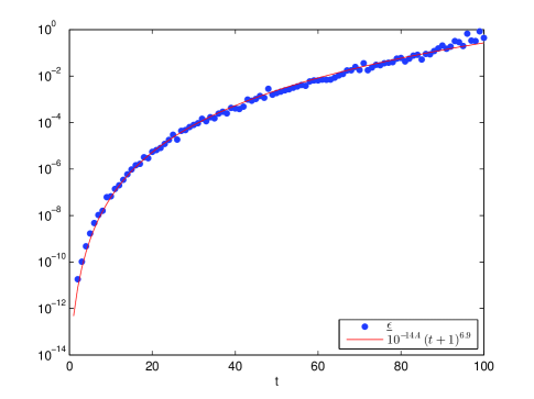
Based on Corollary 9, the lower bounds of ϵitalic-ϵ\epsilon, denoted by ϵ¯¯italic-ϵ\mkern 2.0mu\underline{\mkern-1.5mu\epsilon\mkern-2.5mu}\mkern 4.0mu, for the sets of interval enclosures provided in [15] can be computed. The data containing the sets of interval enclosures for the parameterization of the spherical t𝑡t-designs and relative programs can be downloaded from the website
http://www-ai.math.uni-wuppertal.de/SciComp/SphericalTDesigns. The computational results are shown in Fig 3.1 and Table 3.1.
Refer to caption
Figure 1: ϵ¯¯italic-ϵ\mkern 2.0mu\underline{\mkern-1.5mu\epsilon\mkern-2.5mu}\mkern 4.0mu for t=2,,100𝑡2100t=2,\ldots,100

In Fig. 1.1, we report the lower bounds of ϵitalic-ϵ\epsilon, denoted as ϵ¯¯italic-ϵ\mkern 2.0mu\underline{\mkern-1.5mu\epsilon\mkern-2.5mu}\mkern 4.0mu, for sets of interval enclosures computed in [15] for t=2,,100𝑡2100t=2,\ldots,100 (for t=1𝑡1t=1 we have known that the regular tetrahedron is a spherical t𝑡t-design so that ϵ=0italic-ϵ0\epsilon=0 and we would not consider this case here), based on formula (34). In this figure we also plot a function

y=1014.4(t+1)6.9,𝑦superscript1014.4superscript𝑡16.9y=10^{-14.4}(t+1)^{6.9}, (36)

to approximately estimate the track of ϵ¯¯italic-ϵ\mkern 2.0mu\underline{\mkern-1.5mu\epsilon\mkern-2.5mu}\mkern 4.0mu with respect to t𝑡t. From the figure we can conclude that the lower bound of ϵitalic-ϵ\epsilon grows with the increase of t𝑡t in an order about 6.96.96.9. Additionally, by (34) it is known that the norm of 𝐘(X~N)1𝐘superscriptsubscript~𝑋𝑁1\mathbf{Y}(\tilde{X}_{N})^{-1} is also very important in the process of estimating ϵ¯¯italic-ϵ\mkern 2.0mu\underline{\mkern-1.5mu\epsilon\mkern-2.5mu}\mkern 4.0mu. Fortunately, since the sets of interval enclosures computed in [15] seek to include well-conditioned spherical t𝑡t-designs [2], the growth of lower bounds of ϵitalic-ϵ\epsilon keeps stable for all the t𝑡t considered here.

Table 1: Information for sets of interval enclosures Nsubscript𝑁\mathbb{Z}_{N} for some selected t𝑡t
t𝑡t rad(Nsubscript𝑁\mathbb{Z}_{N}) ρ(N)𝜌subscript𝑁\rho(\mathbb{Z}_{N}) ϵ¯¯italic-ϵ\mkern 2.0mu\underline{\mkern-1.5mu\epsilon\mkern-2.5mu}\mkern 4.0mu ϵitalic-ϵ\epsilon for X~Nsubscript~𝑋𝑁\tilde{X}_{N}
10 1.843454e-12 3.396362e-01 6.748890e-08 6.694645e-14
20 1.515848e-11 1.805783e-01 5.480524e-06 1.783018e-13
30 5.588085e-11 1.249714e-01 7.888659e-05 2.480238e-13
40 1.044163e-10 9.203055e-02 4.043164e-04 5.339063e-13
50 2.199182e-10 7.638945e-02 1.862348e-03 5.057066e-13
60 4.006638e-10 6.302748e-02 6.502352e-03 6.747935e-13
70 6.143914e-10 5.421869e-02 1.820130e-02 8.820722e-13
80 1.220430e-09 4.771142e-02 6.050880e-02 1.151368e-12
90 2.089473e-09 4.264961e-02 2.066649e-01 1.228462e-12
100 2.273791e-09 3.846343e-02 4.420562e-01 1.880540e-12

We also report some information of the interval enclosures and their theoretical lower bounds of ϵitalic-ϵ\epsilon for some selected t𝑡t in Table 3.1. Not only ϵ¯¯italic-ϵ\mkern 2.0mu\underline{\mkern-1.5mu\epsilon\mkern-2.5mu}\mkern 4.0mu but also the radii and separation distances of 𝕏Nsubscript𝕏𝑁\mathbb{X}_{N} are also shown in the table. We can see that the radius of each interval enclosure is far smaller than their separation distance, which means that the assumptions in the above lemmas and theorems are satisfied. For a fixed t𝑡t, the set of center points for each interval ([θ]i,[ϕ]i)Nsubscriptdelimited-[]𝜃𝑖subscriptdelimited-[]italic-ϕ𝑖subscript𝑁([\theta]_{i},[\phi]_{i})\in\mathbb{Z}_{N}, i=1,,N𝑖1𝑁i=1,\ldots,N, denoted as X~N={𝐱~1,𝐱~N}subscript~𝑋𝑁subscript~𝐱1subscript~𝐱𝑁\tilde{X}_{N}=\{\tilde{\mathbf{x}}_{1}\ldots,\tilde{\mathbf{x}}_{N}\}, with 𝐱~isubscript~𝐱𝑖\tilde{\mathbf{x}}_{i} defined by (28), can be regarded as an approximation of a fundamental spherical t𝑡t-design. For each new point set X~Nsubscript~𝑋𝑁\tilde{X}_{N} we compute ϵitalic-ϵ\epsilon by (34) so that the equality holds exactly. As shown in the table, the values of ϵitalic-ϵ\epsilon for each X~Nsubscript~𝑋𝑁\tilde{X}_{N} are all very small positive numbers, and grow with the increase of t𝑡t. This means that X~Nsubscript~𝑋𝑁\tilde{X}_{N} which is selected properly from the interval enclosures is a spherical tϵsubscript𝑡italic-ϵt_{\epsilon}-design.

Remark 10.

To obtain an approximate spherical t𝑡t-design as accurate as possible, in [15] the radius of the set of interval enclosures rad(N)radsubscript𝑁{\rm rad}(\mathbb{Z}_{N}) is computed to a small scale around 1010superscript101010^{-10}. With the introduction of the concept spherical tϵsubscript𝑡italic-ϵt_{\epsilon}-designs, it has been shown that any point set selected in Nsubscript𝑁\mathbb{Z}_{N} is a fundamental spherical tϵsubscript𝑡italic-ϵt_{\epsilon}-design with small enough rad(N)radsubscript𝑁{\rm rad}(\mathbb{Z}_{N}) and ϵ¯¯italic-ϵ\mkern 2.0mu\underline{\mkern-1.5mu\epsilon\mkern-2.5mu}\mkern 4.0mu is increasing in rad(N)radsubscript𝑁{\rm rad}(\mathbb{Z}_{N}). As a result, to reduce the difficulty of computing Nsubscript𝑁\mathbb{Z}_{N}, one may relax rad(N)radsubscript𝑁{\rm rad}(\mathbb{Z}_{N}) to a larger scale with keeping ϵ¯<1¯italic-ϵ1\mkern 2.0mu\underline{\mkern-1.5mu\epsilon\mkern-2.5mu}\mkern 4.0mu<1 holding. Then all point sets selected in Nsubscript𝑁\mathbb{Z}_{N} are still fundamental spherical tϵsubscript𝑡italic-ϵt_{\epsilon}-designs with 0ϵ<10italic-ϵ10\leq\epsilon<1.

4 Worst-case errors of quadrature rules using spherical tϵsubscript𝑡italic-ϵt_{\epsilon}-designs

In this section we will investigate the worst-case errors for quadrature rules with algebraic accuracy t𝑡t using spherical tϵsubscript𝑡italic-ϵt_{\epsilon}-designs in Sobolev spaces which are finite-dimensional rotationally invariant subspaces of C(𝕊2)𝐶superscript𝕊2C(\mathbb{S}^{2}). The bizonal reproducing kernel will be used in the analysis, which has been wildely applied to analyze approximations on the sphere [12, 13, 20, 21, 31]. About equal weight quadrature rules, Brauchart et al [12] recently develop a way to compute their worst-case errors in Sobolev spaces. In this section, we intend to extend their method to non-equal but still positive weight quadrature rules and show the performance of spherical tϵsubscript𝑡italic-ϵt_{\epsilon}-designs in numerical integration.

In this section we follow notations and definitions from [12]. Denote the space of square integrable functions on 𝕊2superscript𝕊2\mathbb{S}^{2} by 𝕃2(𝕊2)subscript𝕃2superscript𝕊2\mathbb{L}_{2}(\mathbb{S}^{2}). Then it is a Hilbert space with the inner product

f,g𝕃2(𝕊d)=𝕊2f(𝐱)g(𝐱)dω(𝐱),f,g𝕃2(𝕊2),formulae-sequencesubscript𝑓𝑔subscript𝕃2superscript𝕊𝑑subscriptsuperscript𝕊2𝑓𝐱𝑔𝐱differential-d𝜔𝐱𝑓𝑔subscript𝕃2superscript𝕊2\langle f,g\rangle_{\mathbb{L}_{2}(\mathbb{S}^{d})}=\int_{\mathbb{S}^{2}}f(\mathbf{x})g(\mathbf{x}){\rm d}\omega(\mathbf{x}),\quad f,g\in\mathbb{L}_{2}(\mathbb{S}^{2}), (37)

and the induced norm as

f𝕃2(𝕊2)=(𝕊2|f(𝐱)|2dω(𝐱))12,f𝕃2(𝕊2).formulae-sequencesubscriptnorm𝑓subscript𝕃2superscript𝕊2superscriptsubscriptsuperscript𝕊2superscript𝑓𝐱2differential-d𝜔𝐱12𝑓subscript𝕃2superscript𝕊2\|f\|_{\mathbb{L}_{2}(\mathbb{S}^{2})}=\left(\int_{\mathbb{S}^{2}}|f(\mathbf{x})|^{2}{\rm d}\omega(\mathbf{x})\right)^{\frac{1}{2}},\quad f\in\mathbb{L}_{2}(\mathbb{S}^{2}). (38)

The Sobolev space s(𝕊2)superscript𝑠superscript𝕊2\mathbb{H}^{s}(\mathbb{S}^{2}) can be defined for s0𝑠0s\geq 0 as the set of all functions f𝕃2(𝕊2)𝑓subscript𝕃2superscript𝕊2f\in\mathbb{L}_{2}(\mathbb{S}^{2}) with whose Laplace-Fourier coefficients

f^,k=f,Y,k𝕃2(𝕊2)=𝕊2f(𝐱)Y,k(𝐱)dω(𝐱),subscript^𝑓𝑘subscript𝑓subscript𝑌𝑘subscript𝕃2superscript𝕊2subscriptsuperscript𝕊2𝑓𝐱subscript𝑌𝑘𝐱differential-d𝜔𝐱\hat{f}_{\ell,k}=\left\langle f,Y_{\ell,k}\right\rangle_{\mathbb{L}_{2}(\mathbb{S}^{2})}=\int_{\mathbb{S}^{2}}f(\mathbf{x})Y_{\ell,k}(\mathbf{x}){\rm d}\omega(\mathbf{x}), (39)

satisfying

=0k=12+1(1+λ)s|f^,k|2<,superscriptsubscript0superscriptsubscript𝑘121superscript1subscript𝜆𝑠superscriptsubscript^𝑓𝑘2\sum_{\ell=0}^{\infty}\sum_{k=1}^{2\ell+1}(1+\lambda_{\ell})^{s}\left|\hat{f}_{\ell,k}\right|^{2}<\infty, (40)

where λ=(+1)subscript𝜆1\lambda_{\ell}=\ell(\ell+1). Obviously, by letting s=0𝑠0s=0 we can obtain 0(𝕊2)=𝕃2(𝕊2)superscript0superscript𝕊2subscript𝕃2superscript𝕊2\mathbb{H}^{0}(\mathbb{S}^{2})=\mathbb{L}_{2}(\mathbb{S}^{2}). Then the norm of s(𝕊2)superscript𝑠superscript𝕊2\mathbb{H}^{s}(\mathbb{S}^{2}) can be defined as

fs=[=0k=12+11α(s)f^,k2]12,subscriptnorm𝑓superscript𝑠superscriptdelimited-[]superscriptsubscript0superscriptsubscript𝑘1211superscriptsubscript𝛼𝑠superscriptsubscript^𝑓𝑘212\|f\|_{\mathbb{H}^{s}}=\left[\sum_{\ell=0}^{\infty}\sum_{k=1}^{2\ell+1}\frac{1}{\alpha_{\ell}^{(s)}}\hat{f}_{\ell,k}^{2}\right]^{\frac{1}{2}}, (41)

where the sequence of positive parameters α(s)superscriptsubscript𝛼𝑠\alpha_{\ell}^{(s)} satisfies

α(s)(1+λ)s(+1)2s.similar-tosuperscriptsubscript𝛼𝑠superscript1subscript𝜆𝑠similar-tosuperscript12𝑠\alpha_{\ell}^{(s)}\sim(1+\lambda_{\ell})^{-s}\sim(\ell+1)^{-2s}. (42)

Correspondingly, the inner product of s(𝕊2)superscript𝑠superscript𝕊2\mathbb{H}^{s}(\mathbb{S}^{2}) can be defined as

f,gs==0k=12+11α(s)f^,kg^,k.subscript𝑓𝑔superscript𝑠superscriptsubscript0superscriptsubscript𝑘1211superscriptsubscript𝛼𝑠subscript^𝑓𝑘subscript^𝑔𝑘\langle f,g\rangle_{\mathbb{H}^{s}}=\sum_{\ell=0}^{\infty}\sum_{k=1}^{2\ell+1}\frac{1}{\alpha_{\ell}^{(s)}}\hat{f}_{\ell,k}\hat{g}_{\ell,k}. (43)

For a point set XNsubscript𝑋𝑁X_{N} and a weight vector 𝐰𝐰\mathbf{w}, we define the numerical quadrature rule and the integral of a function f𝑓f on 𝕊2superscript𝕊2\mathbb{S}^{2} as

Q[XN,𝐰](f):=j=1Nwj4πf(𝐱j),I(f):=𝕊2f(𝐱)dω(𝐱),formulae-sequenceassign𝑄subscript𝑋𝑁𝐰𝑓superscriptsubscript𝑗1𝑁subscript𝑤𝑗4𝜋𝑓subscript𝐱𝑗assign𝐼𝑓subscriptsuperscript𝕊2𝑓𝐱differential-d𝜔𝐱Q[X_{N},\mathbf{w}](f):=\sum_{j=1}^{N}\frac{w_{j}}{4\pi}f(\mathbf{x}_{j}),\quad I(f):=\int_{\mathbb{S}^{2}}f(\mathbf{x}){\rm d}\omega(\mathbf{x}), (44)

The worst-case error of the quadrature rule Q[XN,𝐰]𝑄subscript𝑋𝑁𝐰Q[X_{N},\mathbf{w}] on s(𝕊2)superscript𝑠superscript𝕊2\mathbb{H}^{s}(\mathbb{S}^{2}) can be defined as [12, 20]

Es(Q[XN,𝐰]):=sup{|Q[XN,𝐰](f)I(f)|:fs(𝕊2),fs1}.E_{s}(Q[X_{N},\mathbf{w}]):=\sup\big{\{}\left|Q[X_{N},\mathbf{w}](f)-I(f)\right|:f\in\mathbb{H}^{s}(\mathbb{S}^{2}),\|f\|_{\mathbb{H}^{s}}\leq 1\big{\}}. (45)

The Riesz representation theorem and the additional theorem assure the existence of a reproducing kernel of

Ks(𝐱,𝐲)subscript𝐾𝑠𝐱𝐲\displaystyle K_{s}(\mathbf{x},\mathbf{y}) =\displaystyle= =0(2+1)α(s)P(𝐱𝐲)superscriptsubscript021superscriptsubscript𝛼𝑠subscript𝑃𝐱𝐲\displaystyle\sum_{\ell=0}^{\infty}(2\ell+1)\alpha_{\ell}^{(s)}P_{\ell}(\mathbf{x}\cdot\mathbf{y}) (46)
=\displaystyle= =0k=12+1α(s)Y,k(𝐱)Y,k(𝐲).superscriptsubscript0superscriptsubscript𝑘121superscriptsubscript𝛼𝑠subscript𝑌𝑘𝐱subscript𝑌𝑘𝐲\displaystyle\sum_{\ell=0}^{\infty}\sum_{k=1}^{2\ell+1}\alpha_{\ell}^{(s)}Y_{\ell,k}(\mathbf{x})Y_{\ell,k}(\mathbf{y}).

Together with the property of reproducing kernel Ks(,)subscript𝐾𝑠K_{s}(\cdot,\cdot) defined in (46) and the addition theorem, it is shown in [20] that

(Es(Q[XN,𝐰]))2superscriptsubscript𝐸𝑠𝑄subscript𝑋𝑁𝐰2\displaystyle\big{(}E_{s}(Q[X_{N},\mathbf{w}])\big{)}^{2} =\displaystyle= [supfs(𝕊2)fs1|Q[XN,𝐰](f)I(f)|]2superscriptdelimited-[]subscriptsupremum𝑓superscript𝑠superscript𝕊2subscriptnorm𝑓superscript𝑠1𝑄subscript𝑋𝑁𝐰𝑓𝐼𝑓2\displaystyle\left[\sup_{\mbox{\tiny$\begin{array}[]{c}f\in\mathbb{H}^{s}(\mathbb{S}^{2})\\ \|f\|_{\mathbb{H}^{s}}\leq 1\\ \end{array}$}}\left|Q[X_{N},\mathbf{w}](f)-I(f)\right|\right]^{2}
=\displaystyle= i=1Nwi4πKs(,𝐱)𝕊2Ks(,𝐱)dω(𝐱)s2.superscriptsubscriptnormsuperscriptsubscript𝑖1𝑁subscript𝑤𝑖4𝜋subscript𝐾𝑠𝐱subscriptsuperscript𝕊2subscript𝐾𝑠𝐱differential-d𝜔𝐱superscript𝑠2\displaystyle\left\|\sum_{i=1}^{N}\frac{w_{i}}{4\pi}K_{s}(\cdot,\mathbf{x})-\int_{\mathbb{S}^{2}}K_{s}(\cdot,\mathbf{x}){\rm d}\omega(\mathbf{x})\right\|_{\mathbb{H}^{s}}^{2}.

Assume that Q[XN,𝐰]𝑄subscript𝑋𝑁𝐰Q[X_{N},\mathbf{w}] has algebraic accuracy t𝑡t. Then with the following equality

𝕊2Ks(𝐱,)𝑑ω(𝐱)=α0(s),subscriptsuperscript𝕊2subscript𝐾𝑠𝐱differential-d𝜔𝐱superscriptsubscript𝛼0𝑠\int_{\mathbb{S}^{2}}K_{s}(\mathbf{x},\cdot)d\omega(\mathbf{x})=\alpha_{0}^{(s)},

the worst-case error could be reformulated as

(Es(Q[XN,𝐰]))2superscriptsubscript𝐸𝑠𝑄subscript𝑋𝑁𝐰2\displaystyle(E_{s}(Q[X_{N},\mathbf{w}]))^{2} =\displaystyle= [=1k=12+1α(s)(i=1Nwi4πY,k(𝐱i))2]delimited-[]superscriptsubscript1superscriptsubscript𝑘121superscriptsubscript𝛼𝑠superscriptsuperscriptsubscript𝑖1𝑁subscript𝑤𝑖4𝜋subscript𝑌𝑘subscript𝐱𝑖2\displaystyle\left[\sum_{\ell=1}^{\infty}\sum_{k=1}^{2\ell+1}\alpha_{\ell}^{(s)}\left(\sum_{i=1}^{N}\frac{w_{i}}{4\pi}Y_{\ell,k}(\mathbf{x}_{i})\right)^{2}\right] (48)
=\displaystyle= i=1Nj=1Nwiwj16π2=1k=12+1α(s)Y,k(𝐱i)Y,k(𝐱j).superscriptsubscript𝑖1𝑁superscriptsubscript𝑗1𝑁subscript𝑤𝑖subscript𝑤𝑗16superscript𝜋2superscriptsubscript1superscriptsubscript𝑘121superscriptsubscript𝛼𝑠subscript𝑌𝑘subscript𝐱𝑖subscript𝑌𝑘subscript𝐱𝑗\displaystyle\sum_{i=1}^{N}\sum_{j=1}^{N}\frac{w_{i}w_{j}}{16\pi^{2}}\sum_{\ell=1}^{\infty}\sum_{k=1}^{2\ell+1}\alpha_{\ell}^{(s)}Y_{\ell,k}(\mathbf{x}_{i})Y_{\ell,k}(\mathbf{x}_{j}).

Reproducing kernels for s(𝕊2)superscript𝑠superscript𝕊2\mathbb{H}^{s}(\mathbb{S}^{2}) for s>1𝑠1s>1 can be constructed utilizing powers of distances, provided the power 2s22𝑠22s-2 is not an even integer. Indeed, it is known (cf., e.g., [9, 13]) that the signed power of the distance, with sign (1)L+1superscript1𝐿1(-1)^{L+1} with L:=L(s):=s1assign𝐿𝐿𝑠assign𝑠1L:=L(s):=\lfloor s-1\rfloor, has the following Laplace-Fourier expansion

(1)L+1|𝐱𝐲|2s2=(1)L+1V22s(𝕊2)+=1a(s)(2+1)P(𝐱𝐲),superscript1𝐿1superscript𝐱𝐲2𝑠2superscript1𝐿1subscript𝑉22𝑠superscript𝕊2superscriptsubscript1superscriptsubscript𝑎𝑠21subscript𝑃𝐱𝐲(-1)^{L+1}|\mathbf{x}-\mathbf{y}|^{2s-2}=(-1)^{L+1}V_{2-2s}(\mathbb{S}^{2})+\sum_{\ell=1}^{\infty}a_{\ell}^{(s)}(2\ell+1)P_{\ell}(\mathbf{x}\cdot\mathbf{y}), (49)

where

V22s(𝕊2):=𝕊2𝕊2|𝐱𝐲|2s2dω(𝐱)dω(𝐲)=22s1Γ(3/2)Γ(s)πΓ(1+s),assignsubscript𝑉22𝑠superscript𝕊2subscriptsuperscript𝕊2subscriptsuperscript𝕊2superscript𝐱𝐲2𝑠2differential-d𝜔𝐱differential-d𝜔𝐲superscript22𝑠1Γ32Γ𝑠𝜋Γ1𝑠V_{2-2s}(\mathbb{S}^{2}):=\int_{\mathbb{S}^{2}}\int_{\mathbb{S}^{2}}|\mathbf{x}-\mathbf{y}|^{2s-2}{\rm d}\omega(\mathbf{x}){\rm d}\omega{(\mathbf{y})}=2^{2s-1}\dfrac{\Gamma(3/2)\Gamma(s)}{\sqrt{\pi}\Gamma(1+s)}, (50)
a(s):=V22s(𝕊2)(1)L+1(1s)(1+s),1,formulae-sequenceassignsuperscriptsubscript𝑎𝑠subscript𝑉22𝑠superscript𝕊2superscript1𝐿1subscript1𝑠subscript1𝑠1a_{\ell}^{(s)}:=V_{2-2s}(\mathbb{S}^{2})\dfrac{(-1)^{L+1}(1-s)_{\ell}}{(1+s)_{\ell}},\ \ell\geq 1, (51)

and

(1s)(1+s):=Γ(1+s)Γ(1s)Γ(+1s)Γ(+1+s)Γ(1s)Γ(1+s)2s2s.assignsubscript1𝑠subscript1𝑠Γ1𝑠Γ1𝑠Γ1𝑠Γ1𝑠similar-toΓ1𝑠Γ1𝑠superscript2𝑠similar-tosuperscript2𝑠\frac{(1-s)_{\ell}}{(1+s)_{\ell}}:=\frac{\Gamma(1+s)}{\Gamma(1-s)}\frac{\Gamma(\ell+1-s)}{\Gamma(\ell+1+s)}\sim\frac{\Gamma(1-s)}{\Gamma(1+s)}\ell^{-2s}\sim\ell^{-2s}.

Thus we have

(1)L+2(V22s(𝕊2)|𝐱𝐲|2s2)superscript1𝐿2subscript𝑉22𝑠superscript𝕊2superscript𝐱𝐲2𝑠2\displaystyle(-1)^{L+2}(V_{2-2s}(\mathbb{S}^{2})-|\mathbf{x}-\mathbf{y}|^{2s-2}) =\displaystyle= =1a(s)(2+1)P(𝐱𝐲)superscriptsubscript1superscriptsubscript𝑎𝑠21subscript𝑃𝐱𝐲\displaystyle\sum_{\ell=1}^{\infty}a_{\ell}^{(s)}(2\ell+1)P_{\ell}(\mathbf{x}\cdot\mathbf{y}) (52)
=\displaystyle= =1a(s)k=12+1Y,k(𝐱)Y,k(𝐲).superscriptsubscript1superscriptsubscript𝑎𝑠superscriptsubscript𝑘121subscript𝑌𝑘𝐱subscript𝑌𝑘𝐲\displaystyle\sum_{\ell=1}^{\infty}a_{\ell}^{(s)}\sum_{k=1}^{2\ell+1}Y_{\ell,k}(\mathbf{x})Y_{\ell,k}(\mathbf{y}). (53)

Note that for a(s)superscriptsubscript𝑎𝑠a_{\ell}^{(s)} we have

a(s)22s1Γ(32)Γ(s)π(1)L+1Γ(1+s)2sas,formulae-sequencesimilar-tosuperscriptsubscript𝑎𝑠superscript22𝑠1Γ32Γ𝑠𝜋superscript1𝐿1Γ1𝑠superscript2𝑠asa_{\ell}^{(s)}\sim 2^{2s-1}\dfrac{\Gamma(\frac{3}{2})\Gamma(s)}{\sqrt{\pi}(-1)^{L+1}\Gamma(1+s)}\ell^{-2s}\quad{\rm as}\ \ell\to\infty, (54)

and when 1<s21𝑠21<s\leq 2, which means L=L(s)=0𝐿𝐿𝑠0L=L(s)=0, we have a(s)>0superscriptsubscript𝑎𝑠0a_{\ell}^{(s)}>0 for all =1,1\ell=1,\ldots. Therefore, we regard the left hand side of (52) as the reproducing kernel of s(𝕊2)superscript𝑠superscript𝕊2\mathbb{H}^{s}(\mathbb{S}^{2}), which is

Ks(𝐱,𝐲)=V22s(𝕊2)|𝐱𝐲|2s2,subscript𝐾𝑠𝐱𝐲subscript𝑉22𝑠superscript𝕊2superscript𝐱𝐲2𝑠2K_{s}(\mathbf{x},\mathbf{y})=V_{2-2s}(\mathbb{S}^{2})-|\mathbf{x}-\mathbf{y}|^{2s-2},

and then we obtain

(Es(Q[XN,𝐰]))2=i=1Nj=1Nwiwj16π2(V22s(𝕊2)|𝐱i𝐱j|2s2).superscriptsubscript𝐸𝑠𝑄subscript𝑋𝑁𝐰2superscriptsubscript𝑖1𝑁superscriptsubscript𝑗1𝑁subscript𝑤𝑖subscript𝑤𝑗16superscript𝜋2subscript𝑉22𝑠superscript𝕊2superscriptsubscript𝐱𝑖subscript𝐱𝑗2𝑠2(E_{s}(Q[X_{N},\mathbf{w}]))^{2}=\sum_{i=1}^{N}\sum_{j=1}^{N}\frac{w_{i}w_{j}}{16\pi^{2}}(V_{2-2s}(\mathbb{S}^{2})-|\mathbf{x}_{i}-\mathbf{x}_{j}|^{2s-2}). (55)

For the case s>2𝑠2s>2, we know that a(s)>0superscriptsubscript𝑎𝑠0a_{\ell}^{(s)}>0 does not hold for all =1,1\ell=1,\ldots. In this situation, we let

Ks(𝐱,𝐲)=(1(1)L+1)V22s(𝕊2)+𝒬L(𝐱𝐲)+(1)L+1|𝐱𝐲|2s2,subscript𝐾𝑠𝐱𝐲1superscript1𝐿1subscript𝑉22𝑠superscript𝕊2subscript𝒬𝐿𝐱𝐲superscript1𝐿1superscript𝐱𝐲2𝑠2K_{s}(\mathbf{x},\mathbf{y})=(1-(-1)^{L+1})V_{2-2s}(\mathbb{S}^{2})+\mathcal{Q}_{L}(\mathbf{x}\cdot\mathbf{y})+(-1)^{L+1}|\mathbf{x}-\mathbf{y}|^{2s-2},

with

𝒬L(𝐱𝐲):==1L((1)L+11)a(s)(2+1)P(𝐱𝐲),𝐱,𝐲𝕊2,formulae-sequenceassignsubscript𝒬𝐿𝐱𝐲superscriptsubscript1𝐿superscript1𝐿11superscriptsubscript𝑎𝑠21subscript𝑃𝐱𝐲𝐱𝐲superscript𝕊2\mathcal{Q}_{L}(\mathbf{x}\cdot\mathbf{y}):=\sum_{\ell=1}^{L}((-1)^{L+1-\ell}-1)a_{\ell}^{(s)}(2\ell+1)P_{\ell}(\mathbf{x}\cdot\mathbf{y}),\quad\mathbf{x},\mathbf{y}\in\mathbb{S}^{2},

which changes the signs if the negative coefficients a(s)superscriptsubscript𝑎𝑠a_{\ell}^{(s)} in (49). Hence the worst-case error on s(𝕊2)superscript𝑠superscript𝕊2\mathbb{H}^{s}(\mathbb{S}^{2}) with s>2𝑠2s>2 can be represented as

(Es(Q[XN,𝐰]))2=i=1Nj=1Nwiwj16π2superscriptsubscript𝐸𝑠𝑄subscript𝑋𝑁𝐰2superscriptsubscript𝑖1𝑁superscriptsubscript𝑗1𝑁subscript𝑤𝑖subscript𝑤𝑗16superscript𝜋2\displaystyle(E_{s}(Q[X_{N},\mathbf{w}]))^{2}=\sum_{i=1}^{N}\sum_{j=1}^{N}\frac{w_{i}w_{j}}{16\pi^{2}} (𝒬L(𝐱i𝐱j)+(1)L+1|𝐱i𝐱j|2s2\displaystyle\left(\mathcal{Q}_{L}(\mathbf{x}_{i}\cdot\mathbf{x}_{j})+(-1)^{L+1}|\mathbf{x}_{i}-\mathbf{x}_{j}|^{2s-2}\right. (56)
(1)L+1V22s(𝕊2)).\displaystyle\left.-(-1)^{L+1}V_{2-2s}(\mathbb{S}^{2})\right).

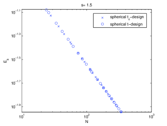
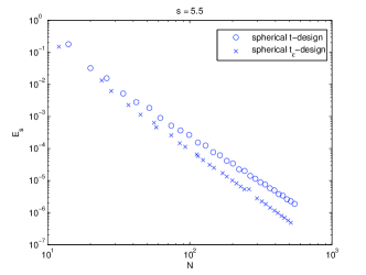
In what follows we will compute the worst-case errors of quadrature rules using spherical tϵsubscript𝑡italic-ϵt_{\epsilon}-designs with algebraic accuracy t𝑡t. In this experiment we choose ϵ=0.1italic-ϵ0.1\epsilon=0.1 for spherical tϵsubscript𝑡italic-ϵt_{\epsilon}-designs and use (12) to find a spherical tϵsubscript𝑡italic-ϵt_{\epsilon}-design, which is a system of nonlinear equations. The system can be solved by minimizing its least squares form using a smoothing trust-region filter method proposed in [14]. Note that the number of points needed for constructing spherical tϵsubscript𝑡italic-ϵt_{\epsilon}-designs may decrease with the increase of ϵitalic-ϵ\epsilon. Thus in the computation of spherical tϵsubscript𝑡italic-ϵt_{\epsilon}-designs we always attempt to find the one with a possible minimal number of points, denoted as N(t,ϵ)𝑁𝑡italic-ϵN(t,\epsilon). The detailed process for finding spherical tϵsubscript𝑡italic-ϵt_{\epsilon}-designs can be found in [14]. In the numerical test of computation of spherical tϵsubscript𝑡italic-ϵt_{\epsilon}-designs it is found that a possible minimal number of points satisfies (t+1)2/3+1N(t,ϵ)(t+2)2/2+1superscript𝑡1231𝑁𝑡italic-ϵsuperscript𝑡2221\lceil(t+1)^{2}/3\rceil+1\leq N(t,\epsilon)\leq\lceil(t+2)^{2}/2\rceil+1. In the numerical test in current and next sections, the spherical tϵsubscript𝑡italic-ϵt_{\epsilon}-designs are chosen with N=N(t,ϵ)𝑁𝑁𝑡italic-ϵN=N(t,\epsilon).

Refer to caption
(a) s=1.5𝑠1.5s=1.5
Refer to caption
(b) s=5.5𝑠5.5s=5.5
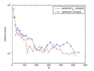
Figure 2: Worst-case errors for spherical t0.1subscript𝑡0.1t_{0.1}-designs and spherical t𝑡t-designs

The worst-case errors of quadrature rules using spherical t0.1subscript𝑡0.1t_{0.1}-designs in s(𝕊2)superscript𝑠superscript𝕊2\mathbb{H}^{s}(\mathbb{S}^{2}) for s=1.5𝑠1.5s=1.5 are illustrated in Fig. 2(a). For comparison, the worst-case errors for quadrature rules using approximate spherical t𝑡t-designs computed in [27] will also be implemented. For all spherical t0.1subscript𝑡0.1t_{0.1}-designs, the worst-case error with s=1.5𝑠1.5s=1.5 is calculated using (55) and the distance kernel, and for spherical t𝑡t-designs the worst-case errors are calculated by relative results in [12]. From the figure we can see that in this case, the computed worst-case errors of approximate spherical t𝑡t-designs and spherical t0.1subscript𝑡0.1t_{0.1}-designs essentially lie on the same curve, which remains as a conjecture that the worst-case errors of both spherical t𝑡t-designs and spherical tϵsubscript𝑡italic-ϵt_{\epsilon}-designs decay in the same speed with respect to the number of points in the case s<2𝑠2s<2 on 𝕊2superscript𝕊2\mathbb{S}^{2}. Figure 2(b) plots the worst-case errors for both spherical t𝑡t-designs and spherical t0.1subscript𝑡0.1t_{0.1}-designs with s=5.5𝑠5.5s=5.5. From the figure we can see that the worst-case errors of spherical t0.1subscript𝑡0.1t_{0.1}-designs decay faster than the ones of spherical t𝑡t-design with respect to the number of points.

5 Polynomial approximation on the sphere using spherical tϵsubscript𝑡italic-ϵt_{\epsilon}-designs

5.1 Regularized weighted least squares approximation using spherical tϵsubscript𝑡italic-ϵt_{\epsilon}-designs

In this section we consider the restoration of a continuous function fC(𝕊2)𝑓𝐶superscript𝕊2f\in C(\mathbb{S}^{2}) from its noisy values fδsuperscript𝑓𝛿f^{\delta} given at N𝑁N points XN={𝐱1,,𝐱N}𝕊2subscript𝑋𝑁subscript𝐱1subscript𝐱𝑁superscript𝕊2X_{N}=\{\mathbf{x}_{1},\ldots,\mathbf{x}_{N}\}\subset\mathbb{S}^{2} by the l2l1subscript𝑙2subscript𝑙1l_{2}-l_{1} regularized weighted discrete least squares form

minα,k12j=1Nμj(=0Lk=12k+1α,kY,k(𝐱j)fδ(𝐱j))2+λ=0Lk=12+1|β,kα,k|subscriptsubscript𝛼𝑘12superscriptsubscript𝑗1𝑁subscript𝜇𝑗superscriptsuperscriptsubscript0𝐿superscriptsubscript𝑘12𝑘1subscript𝛼𝑘subscript𝑌𝑘subscript𝐱𝑗superscript𝑓𝛿subscript𝐱𝑗2𝜆superscriptsubscript0𝐿superscriptsubscript𝑘121subscript𝛽𝑘subscript𝛼𝑘\min_{\alpha_{\ell,k}\in\mathbb{R}}\frac{1}{2}\sum_{j=1}^{N}\mu_{j}(\sum_{\ell=0}^{L}\sum_{k=1}^{2k+1}\alpha_{\ell,k}Y_{\ell,k}(\mathbf{x}_{j})-f^{\delta}(\mathbf{x}_{j}))^{2}+\lambda\sum_{\ell=0}^{L}\sum_{k=1}^{2\ell+1}|\beta_{\ell,k}\alpha_{\ell,k}| (57)

where μj>0subscript𝜇𝑗0\mu_{j}>0, j=1,,N𝑗1𝑁j=1,\ldots,N are the weights for each term of the least squares model, λ>0𝜆0\lambda>0 is the regularization parameter, and β,k0subscript𝛽𝑘0\beta_{\ell,k}\geq 0, =0,,L,k=1,,2+1formulae-sequence0𝐿𝑘121\ell=0,\ldots,L,\ k=1,\ldots,2\ell+1 are usually chosen with the meaning of certain polynomial operators such as Laplace-Beltrami operator and filtered operator [3, 28]. In [23] both a priori choice based physical reason in satellite gravity gradiometry problem and a posteriori choice based on reproducing kernel theory are considered to choose β,ksubscript𝛽𝑘\beta_{\ell,k}.

Note that {Y,k,k=1,,2+1,=0,,L}formulae-sequencesubscript𝑌𝑘𝑘1210𝐿\{Y_{\ell,k},\ k=1,\ldots,2\ell+1,\ \ell=0,\ldots,L\} is a basis of Lsubscript𝐿\mathbb{P}_{L}. Problem (57) is to find a good approximation of f𝑓f in Lsubscript𝐿\mathbb{P}_{L} in the form

pL,N(𝐱)==0Lk=12+1α,kY,k(𝐱).subscript𝑝𝐿𝑁𝐱superscriptsubscript0𝐿superscriptsubscript𝑘121subscript𝛼𝑘subscript𝑌𝑘𝐱p_{L,N}(\mathbf{x})=\sum_{\ell=0}^{L}\sum_{k=1}^{2\ell+1}\alpha_{\ell,k}Y_{\ell,k}(\mathbf{x}).

Let the entries of matrix 𝐘LN×(L+1)2subscript𝐘𝐿superscript𝑁superscript𝐿12\mathbf{Y}_{L}\in\mathbb{R}^{N\times(L+1)^{2}} be

(𝐘L)i,2+k=Y,k(𝐱i),i=1,,N,=0,,L,k=1,,2+1,formulae-sequencesubscriptsubscript𝐘𝐿𝑖superscript2𝑘subscript𝑌𝑘subscript𝐱𝑖formulae-sequence𝑖1𝑁formulae-sequence0𝐿𝑘121(\mathbf{Y}_{L})_{i,\ell^{2}+k}=Y_{\ell,k}(\mathbf{x}_{i}),\ \ i=1,\ldots,N,\ \ell=0,\ldots,L,\ k=1,\ldots,2\ell+1,

and 𝐟δ=(fδ(𝐱1),,fδ(𝐱N))Tsuperscript𝐟𝛿superscriptsuperscript𝑓𝛿subscript𝐱1superscript𝑓𝛿subscript𝐱𝑁𝑇\mathbf{f}^{\delta}=(f^{\delta}(\mathbf{x}_{1}),\ldots,f^{\delta}(\mathbf{x}_{N}))^{T}. Problem (57) can be reformulated as

minα(L+1)212𝚲12(𝐘Lα𝐟δ)22+λ𝐃α1,subscript𝛼superscriptsuperscript𝐿1212subscriptsuperscriptnormsuperscript𝚲12subscript𝐘𝐿𝛼superscript𝐟𝛿22𝜆subscriptnorm𝐃𝛼1\quad\min_{\alpha\in\mathbb{R}^{(L+1)^{2}}}\frac{1}{2}\|\mathbf{\Lambda}^{\frac{1}{2}}(\mathbf{Y}_{L}\alpha-\mathbf{f}^{\delta})\|^{2}_{2}+\lambda\|\mathbf{D}\alpha\|_{1}, (58)

where

𝚲=[μ1μN]N×N,𝚲delimited-[]subscript𝜇1missing-subexpressionmissing-subexpressionmissing-subexpressionmissing-subexpressionmissing-subexpressionmissing-subexpressionsubscript𝜇𝑁superscript𝑁𝑁\mathbf{\Lambda}=\left[\begin{array}[]{ccc}\mu_{1}&&\\ &\ddots&\\ &&\mu_{N}\\ \end{array}\right]\in\mathbb{R}^{N\times N},

and 𝐃𝐃\mathbf{D} is a diagonal matrix satisfying 𝐃2+k,2+k=β,ksubscript𝐃superscript2𝑘superscript2𝑘subscript𝛽𝑘\mathbf{D}_{\ell^{2}+k,\ell^{2}+k}=\beta_{\ell,k} with β,k0subscript𝛽𝑘0\beta_{\ell,k}\geq 0. For polynomial approximation on the sphere, an l2subscript𝑙2l_{2}-regularized weighted least squares model has also been considered [3, 23]

minα(L+1)212𝚲12(𝐘Lα𝐟δ)22+λ𝐃α22.subscript𝛼superscriptsuperscript𝐿1212subscriptsuperscriptnormsuperscript𝚲12subscript𝐘𝐿𝛼superscript𝐟𝛿22𝜆superscriptsubscriptnorm𝐃𝛼22\min_{\alpha\in\mathbb{R}^{(L+1)^{2}}}\frac{1}{2}\|\mathbf{\Lambda}^{\frac{1}{2}}(\mathbf{Y}_{L}\alpha-\mathbf{f}^{\delta})\|^{2}_{2}+\lambda\|\mathbf{D}\alpha\|_{2}^{2}. (59)

The regularization of this model is of l2subscript𝑙2l_{2} norm, which can be seen as a measure of energy. It is known that the l1subscript𝑙1l_{1} regularization has desirable properties in approximation of nonsmooth continuous functions. An l1subscript𝑙1l_{1} regularization term is preferable to be considered here. By choosing a suitable penalization term, the l2l1subscript𝑙2subscript𝑙1l_{2}-l_{1} regularized model is usually supposed to achieve a more sparse solution than the l2l2subscript𝑙2subscript𝑙2l_{2}-l_{2} regularized one, which means that the target function is approximated by less basis spherical polynomials. Additionally, for functions which are globally continuous but locally non-differentiable on the sphere, the l2l1subscript𝑙2subscript𝑙1l_{2}-l_{1} regularization is better than the l2l2subscript𝑙2subscript𝑙2l_{2}-l_{2} regularization.

Theorem 11.

Let XNsubscript𝑋𝑁X_{N} be a spherical tϵsubscript𝑡italic-ϵt_{\epsilon}-design and 𝐰𝐰\mathbf{w} be the vector of weights satisfying (2) and (3) with respect to XNsubscript𝑋𝑁X_{N}. Let L0𝐿0L\geq 0. For model (58) set μj=wjsubscript𝜇𝑗subscript𝑤𝑗\mu_{j}=w_{j} for j=1,,N𝑗1𝑁j=1,\ldots,N. Then

𝐇L=𝐘LT𝚲𝐘L=𝐈(L+1)2,subscript𝐇𝐿subscriptsuperscript𝐘𝑇𝐿𝚲subscript𝐘𝐿subscript𝐈superscript𝐿12\mathbf{H}_{L}=\mathbf{Y}^{T}_{L}\mathbf{\Lambda}\mathbf{Y}_{L}=\mathbf{I}_{(L+1)^{2}}, (60)

and (58) has the unique solution

α,k=max{0,s,kλβ,k}+min{0,s,k+λβ,k},subscript𝛼𝑘0subscript𝑠𝑘𝜆subscript𝛽𝑘0subscript𝑠𝑘𝜆subscript𝛽𝑘\alpha_{\ell,k}=\max\{0,s_{\ell,k}-\lambda\beta_{\ell,k}\}+\min\{0,s_{\ell,k}+\lambda\beta_{\ell,k}\}, (61)

for =0,,L0𝐿\ell=0,\ldots,L, k=1,,2k+1𝑘12𝑘1k=1,\ldots,2k+1, where s,k=i=1NwiY,k(𝐱i)fδ(𝐱i)subscript𝑠𝑘superscriptsubscript𝑖1𝑁subscript𝑤𝑖subscript𝑌𝑘subscript𝐱𝑖superscript𝑓𝛿subscript𝐱𝑖s_{\ell,k}=\sum_{i=1}^{N}w_{i}Y_{\ell,k}(\mathbf{x}_{i})f^{\delta}(\mathbf{x}_{i}).

Proof.

Note that when XNsubscript𝑋𝑁X_{N} is a spherical tϵsubscript𝑡italic-ϵt_{\epsilon}-design,

(𝐇L)2+k,()2+ksubscriptsubscript𝐇𝐿superscript2𝑘superscriptsuperscript2superscript𝑘\displaystyle\left(\mathbf{H}_{L}\right)_{\ell^{2}+k,(\ell^{\prime})^{2}+k^{\prime}} =\displaystyle= i=1NwiY,k(𝐱i)Y,k(𝐱i)superscriptsubscript𝑖1𝑁subscript𝑤𝑖subscript𝑌𝑘subscript𝐱𝑖subscript𝑌superscriptsuperscript𝑘subscript𝐱𝑖\displaystyle\sum_{i=1}^{N}w_{i}Y_{\ell,k}(\mathbf{x}_{i})Y_{\ell^{\prime},k^{\prime}}(\mathbf{x}_{i}) (62)
=\displaystyle= 𝕊2Y,k(𝐱)Y,k(𝐱)dω(𝐱)=δδkk,subscriptsuperscript𝕊2subscript𝑌𝑘𝐱subscript𝑌superscriptsuperscript𝑘𝐱differential-d𝜔𝐱subscript𝛿superscriptsubscript𝛿𝑘superscript𝑘\displaystyle\int_{\mathbb{S}^{2}}Y_{\ell,k}(\mathbf{x})Y_{\ell^{\prime},k^{\prime}}(\mathbf{x}){\rm d}\omega(\mathbf{x})=\delta_{\ell\ell^{\prime}}\delta_{kk^{\prime}},

where the third equality is established by the orthonormality of spherical harmonics. Problem (58) is strictly convex by the fact that 𝐇Lsubscript𝐇𝐿\mathbf{H}_{L} is nonsingular and so it has a unique optimal solution. Since A(α)=12𝚲12(𝐘Lα𝐟δ)22𝐴𝛼12subscriptsuperscriptnormsuperscript𝚲12subscript𝐘𝐿𝛼superscript𝐟𝛿22A(\alpha)=\frac{1}{2}\|\mathbf{\Lambda}^{\frac{1}{2}}(\mathbf{Y}_{L}\alpha-\mathbf{f}^{\delta})\|^{2}_{2} is strictly differentiable, by deriving the first optimality condition of (58) and Corollary 1 in [16, Section 2.3], we obtain that its unique optimal solution satisfies

0𝐇Lα𝐘LT𝐖𝐟δ+λ(𝐃α1),0subscript𝐇𝐿𝛼subscriptsuperscript𝐘𝑇𝐿superscript𝐖𝐟𝛿𝜆subscriptnorm𝐃𝛼10\in\mathbf{H}_{L}\alpha-\mathbf{Y}^{T}_{L}\mathbf{W}\mathbf{f}^{\delta}+\lambda\partial(\|\mathbf{D}\alpha\|_{1}), (63)

where ()\partial(\cdot) denotes the subdifferential. By (62) which implies 𝐇L=𝐈(L+1)2subscript𝐇𝐿subscript𝐈superscript𝐿12\mathbf{H}_{L}=\mathbf{I}_{(L+1)^{2}} and the fact that 𝐃𝐃\mathbf{D} is diagonal, problem (63) is separable and thus α𝛼\alpha is a solution of (63) if and only if it is a solution of

0α,ks,k+λβ,k|α,k|,=0,,L,k=1,,2+1.formulae-sequence0subscript𝛼𝑘subscript𝑠𝑘𝜆subscript𝛽𝑘subscript𝛼𝑘formulae-sequence0𝐿𝑘1210\in\alpha_{\ell,k}-s_{\ell,k}+\lambda\beta_{\ell,k}\partial|\alpha_{\ell,k}|,\quad\ell=0,\ldots,L,k=1,\ldots,2\ell+1. (64)

Denote τ,k=|α,k|subscript𝜏𝑘subscript𝛼𝑘\tau_{\ell,k}=\partial|\alpha_{\ell,k}| and hence 1τ,k11subscript𝜏𝑘1-1\leq\tau_{\ell,k}\leq 1. Let α,ksuperscriptsubscript𝛼𝑘\alpha_{\ell,k}^{\ast} be the optimal solution of (64) with corresponding \ell and k𝑘k and hence

α,k=s,kλβ,kτ,kwithτ,k[1,1].formulae-sequencesuperscriptsubscript𝛼𝑘subscript𝑠𝑘𝜆subscript𝛽𝑘subscript𝜏𝑘withsubscript𝜏𝑘11\alpha_{\ell,k}^{\ast}=s_{\ell,k}-\lambda\beta_{\ell,k}\tau_{\ell,k}\quad{\rm with}\ \tau_{\ell,k}\in[-1,1]. (65)

When s,k>λβ,ksubscript𝑠𝑘𝜆subscript𝛽𝑘s_{\ell,k}>\lambda\beta_{\ell,k} we can set τ,k=1subscript𝜏𝑘1\tau_{\ell,k}=1 and obtain

α,k=s,kλβ,k>0,subscriptsuperscript𝛼𝑘subscript𝑠𝑘𝜆subscript𝛽𝑘0\alpha^{\ast}_{\ell,k}=s_{\ell,k}-\lambda\beta_{\ell,k}>0,

which together with β,k0subscript𝛽𝑘0\beta_{\ell,k}\geq 0 satisfies (61) and (65). When s,k<λβ,ksubscript𝑠𝑘𝜆subscript𝛽𝑘s_{\ell,k}<-\lambda\beta_{\ell,k} similarly we set τ,k=1subscript𝜏𝑘1\tau_{\ell,k}=-1 and get

α,k=s,k+λβ,k<0,subscriptsuperscript𝛼𝑘subscript𝑠𝑘𝜆subscript𝛽𝑘0\alpha^{\ast}_{\ell,k}=s_{\ell,k}+\lambda\beta_{\ell,k}<0,

which also satisfies (61) and (65). Then when s,k[λβ,k,λβ,k]subscript𝑠𝑘𝜆subscript𝛽𝑘𝜆subscript𝛽𝑘s_{\ell,k}\in[-\lambda\beta_{\ell,k},\lambda\beta_{\ell,k}] we set τ,k=s,kλβ,k[1,1]subscript𝜏𝑘subscript𝑠𝑘𝜆subscript𝛽𝑘11\tau_{\ell,k}=\frac{s_{\ell,k}}{\lambda\beta_{\ell,k}}\in[-1,1] and get that

α,k=0,subscriptsuperscript𝛼𝑘0\alpha^{\ast}_{\ell,k}=0,

which also satisfies (61) and (65). Hence the theorem is proved. ∎

Denote the approximation residual as A(α)=j=1N(pL,N(𝐱j)fδ(𝐱j))2𝐴𝛼superscriptsubscript𝑗1𝑁superscriptsubscript𝑝𝐿𝑁subscript𝐱𝑗superscript𝑓𝛿subscript𝐱𝑗2A(\alpha)=\sum_{j=1}^{N}(p_{L,N}(\mathbf{x}_{j})-f^{\delta}(\mathbf{x}_{j}))^{2}. Let α(λ)superscript𝛼𝜆\alpha^{\ast}(\lambda) be the optimal solution of (58) with different regularized parameters λ𝜆\lambda. The following proposition indicates that A(α(λ))𝐴superscript𝛼𝜆A(\alpha^{\ast}(\lambda)) is monotonically increasing with respect to λ𝜆\lambda.

Proposition 12.

Let XNϵsuperscriptsubscript𝑋𝑁italic-ϵX_{N}^{\epsilon} be a spherical tϵsubscript𝑡italic-ϵt_{\epsilon}-design with t2L𝑡2𝐿t\geq 2L and μj=wjsubscript𝜇𝑗subscript𝑤𝑗\mu_{j}=w_{j} for j=1,,N𝑗1𝑁j=1,\ldots,N. Then A(α(λ))𝐴superscript𝛼𝜆A(\alpha^{\ast}(\lambda)) is increasing in λ𝜆\lambda.

Proof.

Let λ𝜆\lambda, λ~~𝜆\tilde{\lambda} be given with 0<λλ~0𝜆~𝜆0<\lambda\leq\tilde{\lambda} and denote the optimal solution of problem (58) with λ𝜆\lambda, λ~~𝜆\tilde{\lambda} as αsuperscript𝛼\alpha^{\ast}, α~superscript~𝛼\tilde{\alpha}^{\ast} respectively. Denote E(λ,α)=λ𝐃α1𝐸𝜆𝛼𝜆subscriptnorm𝐃𝛼1E(\lambda,\alpha)=\lambda\|\mathbf{D}\alpha\|_{1} and the minimization property of (58) for λ𝜆\lambda gives

A(α)+E(λ,α)A(α~)+E(λ,α~),𝐴superscript𝛼𝐸𝜆superscript𝛼𝐴superscript~𝛼𝐸𝜆superscript~𝛼A(\alpha^{\ast})+E(\lambda,\alpha^{\ast})\leq A(\tilde{\alpha}^{\ast})+E(\lambda,\tilde{\alpha}^{\ast}), (66)

which implies that

A(α)A(α~)E(λ,α~)E(λ,α).𝐴superscript𝛼𝐴superscript~𝛼𝐸𝜆superscript~𝛼𝐸𝜆superscript𝛼A(\alpha^{\ast})-A(\tilde{\alpha}^{\ast})\leq E(\lambda,\tilde{\alpha}^{\ast})-E(\lambda,\alpha^{\ast}). (67)

From (61) we have

α,k={s,kλβ,k,s,k>λβ,ks,k+λβ,k,s,k<λβ,k0.λβ,ks,kλβ,ksubscriptsuperscript𝛼𝑘casessubscript𝑠𝑘𝜆subscript𝛽𝑘subscript𝑠𝑘𝜆subscript𝛽𝑘subscript𝑠𝑘𝜆subscript𝛽𝑘subscript𝑠𝑘𝜆subscript𝛽𝑘0𝜆subscript𝛽𝑘subscript𝑠𝑘𝜆subscript𝛽𝑘\alpha^{\ast}_{\ell,k}=\left\{\begin{array}[]{cl}s_{\ell,k}-\lambda\beta_{\ell,k},&\quad\quad s_{\ell,k}>\lambda\beta_{\ell,k}\\ s_{\ell,k}+\lambda\beta_{\ell,k},&\quad\quad s_{\ell,k}<-\lambda\beta_{\ell,k}\\ 0.&\quad\quad-\lambda\beta_{\ell,k}\leq s_{\ell,k}\leq\lambda\beta_{\ell,k}\\ \end{array}\right. (68)

Since λβ,k0𝜆subscript𝛽𝑘0\lambda\beta_{\ell,k}\geq 0, we have |α,k|=max(0,|s,k|λβ,k)subscriptsuperscript𝛼𝑘0subscript𝑠𝑘𝜆subscript𝛽𝑘|\alpha^{\ast}_{\ell,k}|=\max(0,|s_{\ell,k}|-\lambda\beta_{\ell,k}). Together by the fact that

E(λ,α)=λ=0Lk=12+1β,k|α,k|,𝐸𝜆superscript𝛼𝜆superscriptsubscript0𝐿superscriptsubscript𝑘121subscript𝛽𝑘subscriptsuperscript𝛼𝑘E(\lambda,\alpha^{\ast})=\lambda\sum_{\ell=0}^{L}\sum_{k=1}^{2\ell+1}\beta_{\ell,k}|\alpha^{\ast}_{\ell,k}|,

we have

|α~,k|=max(0,|s,k|λ~β,k)max(0,|s,k|λβ,k)=|α,k|.subscriptsuperscript~𝛼𝑘0subscript𝑠𝑘~𝜆subscript𝛽𝑘0subscript𝑠𝑘𝜆subscript𝛽𝑘subscriptsuperscript𝛼𝑘|\tilde{\alpha}^{\ast}_{\ell,k}|=\max(0,|s_{\ell,k}|-\tilde{\lambda}\beta_{\ell,k})\leq\max(0,|s_{\ell,k}|-\lambda\beta_{\ell,k})=|\alpha^{\ast}_{\ell,k}|.

Hence it is obtained that E(λ,α~)E(λ,α)𝐸𝜆superscript~𝛼𝐸𝜆superscript𝛼E(\lambda,\tilde{\alpha}^{\ast})\leq E(\lambda,\alpha^{\ast}). Together with (66) we complete the proof. ∎

5.2 Numerical experiments

In this subsection we report the numerical results to test the efficiency of the l2l1subscript𝑙2subscript𝑙1l_{2}-l_{1} regularized model (58) using spherical tϵsubscript𝑡italic-ϵt_{\epsilon}-designs.

Example 5.1. In the first numerical test, the target function is selected as spherical polynomials with degree no higher than L𝐿L. Obviously using both models (58) and (59) the target function can be exactly restored when λ=0𝜆0\lambda=0 and the data 𝐟δsuperscript𝐟𝛿\mathbf{f}^{\delta} is noise free and the optimal values of the two models equal to 0 in such case. However, due to the noise in the data vector 𝐟δsuperscript𝐟𝛿\mathbf{f}^{\delta}, it is necessary to use the regularization models.

In this experiment we will use the spherical t0.1subscript𝑡0.1t_{0.1}-designs which is calculated by solving a system of nonlinear equation (12) and the approximate spherical t𝑡t-designs proposed in [27] as the point set for polynomial approximation. Both the uniform errors and 𝕃2subscript𝕃2\mathbb{L}_{2} errors are recorded to measure the approximation quality. We choose a large-scaled and well distributed point set Xt𝕊2subscript𝑋𝑡superscript𝕊2X_{t}\subset\mathbb{S}^{2} to be the test set and use it to estimate the errors. Then the uniform error and 𝕃2subscript𝕃2\mathbb{L}_{2} error of the approximation are estimated by

fpL,NC(𝕊2)max𝐱iXt|f(𝐱i)pL,N(𝐱i)|,subscriptnorm𝑓subscript𝑝𝐿𝑁𝐶superscript𝕊2subscriptsubscript𝐱𝑖subscript𝑋𝑡𝑓subscript𝐱𝑖subscript𝑝𝐿𝑁subscript𝐱𝑖\|f-p_{L,N}\|_{C(\mathbb{S}^{2})}\approx\max_{\mathbf{x}_{i}\in X_{t}}|f(\mathbf{x}_{i})-p_{L,N}(\mathbf{x}_{i})|, (69)

and

fpL,N𝕃2(4πNti=1Nt(f(𝐱i)pL,N(𝐱i))2)12,subscriptnorm𝑓subscript𝑝𝐿𝑁subscript𝕃2superscript4𝜋subscript𝑁𝑡superscriptsubscript𝑖1subscript𝑁𝑡superscript𝑓subscript𝐱𝑖subscript𝑝𝐿𝑁subscript𝐱𝑖212\|f-p_{L,N}\|_{\mathbb{L}_{2}}\approx\left(\dfrac{4\pi}{N_{t}}\sum_{i=1}^{N_{t}}(f(\mathbf{x}_{i})-p_{L,N}(\mathbf{x}_{i}))^{2}\right)^{\frac{1}{2}}, (70)

where Ntsubscript𝑁𝑡N_{t} denotes the number of points 𝐱isubscript𝐱𝑖\mathbf{x}_{i} in Xtsubscript𝑋𝑡X_{t}. In this experiment, we choose Xtsubscript𝑋𝑡X_{t} to be an equal area partitioning point set [25] with 105superscript10510^{5} points. The matrix 𝐃𝐃\mathbf{D} in the experiment is always selected as β,k=(+1)subscript𝛽𝑘1\beta_{\ell,k}=\ell(\ell+1) for =0,,L,k=2+1formulae-sequence0𝐿𝑘21\ell=0,\ldots,L,\ k=2\ell+1, inspired by the Laplace-Beltrami operator, see [3].
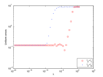
Refer to caption
(a) Uniform Errors with different λ𝜆\lambda for δ=0.1𝛿0.1\delta=0.1
Refer to caption
(b) 𝕃2subscript𝕃2\mathbb{L}_{2} errors with different λ𝜆\lambda for δ=0.1𝛿0.1\delta=0.1
Refer to caption
(c) Minimal uniform errors with different noise scales δ𝛿\delta
Refer to caption
(d) Minimal 𝕃2subscript𝕃2\mathbb{L}_{2} errors with different noise scales δ𝛿\delta
Figure 3: Errors for restoring 181818-degree polynomial

Fig. 5.1 shows the approximation errors using both l2l1subscript𝑙2subscript𝑙1l_{2}-l_{1} model (58) and l2l2subscript𝑙2subscript𝑙2l_{2}-l_{2} model (59) with different λ𝜆\lambda and different noise scales δ𝛿\delta. The noise of the data 𝐟δsuperscript𝐟𝛿\mathbf{f}^{\delta} obeys a uniform distribution in [δ,δ]𝛿𝛿[-\delta,\delta]. In this numerical experiment a spherical 370.1subscript370.137_{0.1}-design with only 514 points, which is much less than (t+1)22superscript𝑡122\lceil\frac{(t+1)^{2}}{2}\rceil, is applied to approximate a randomly generated spherical polynomial with degree 372=1837218\lfloor\frac{37}{2}\rfloor=18 (The polynomial is generated with all its Fourier coefficients obeying the standard normal distribution). The regularization parameter λ𝜆\lambda is chosen from 1020superscript102010^{-20} to 100.5superscript100.510^{0.5}. Fig. 5.1 (a)(b) give the errors of the approximation with different λ𝜆\lambda for δ=0.1𝛿0.1\delta=0.1 using the two models. From the two sub-figures it can be seen that model (58) can restore the 181818-degree polynomial more accurately than model (59). The minimal error with respect to different λ𝜆\lambda can be achieved at about λ=106𝜆superscript106\lambda=10^{-6}. Fig. 5.1 (c)(d) show the errors of the restoration results with different noise scales. It can be seen that the model (58) performs better in each noise scale than (59).

Example 5.2. In the second numerical experiment we test the numerical performance of model (58) using spherical tϵsubscript𝑡italic-ϵt_{\epsilon}-designs and spherical t𝑡t-designs. We select the Franke function [24]

f1(𝐱)=f(x,y,z)=0.75exp((9x2)2/4(9y2)2/4(9z2)2/4)+0.75exp((9x+1)2/49(9y+1)/10(9z+1)/10)+0.5exp((9x7)2/4(9y3)2/4(9z5)2/4)0.2exp((9x4)2(9y7)2(9z5)2),(x,y,z)𝕊2formulae-sequencesubscript𝑓1𝐱𝑓𝑥𝑦𝑧0.75superscript9𝑥224superscript9𝑦224superscript9𝑧2240.75superscript9𝑥12499𝑦1109𝑧1100.5superscript9𝑥724superscript9𝑦324superscript9𝑧5240.2superscript9𝑥42superscript9𝑦72superscript9𝑧52𝑥𝑦𝑧superscript𝕊2\begin{split}f_{1}(\mathbf{x})=&f(x,y,z)=0.75\exp(-(9x-2)^{2}/4-(9y-2)^{2}/4-(9z-2)^{2}/4)\\ &+0.75\exp(-(9x+1)^{2}/49-(9y+1)/10-(9z+1)/10)\\ &+0.5\exp(-(9x-7)^{2}/4-(9y-3)^{2}/4-(9z-5)^{2}/4)\\ &-0.2\exp(-(9x-4)^{2}-(9y-7)^{2}-(9z-5)^{2}),\ (x,y,z)\in\mathbb{S}^{2}\end{split} (71)

to be the target function which is not a spherical polynomial but continuously differentiable on the whole sphere. We set ϵ=0.1italic-ϵ0.1\epsilon=0.1 and also δ=0.1𝛿0.1\delta=0.1 in this experiment and the scheme of choosing λ𝜆\lambda is the same as in Example 5.1. For spherical t0.1subscript𝑡0.1t_{0.1}-designs we select those point sets constructed with possible least points. As is mentioned above, a spherical t0.1subscript𝑡0.1t_{0.1}-design may be constructed using less than (t+1)22superscript𝑡122\lceil\frac{(t+1)^{2}}{2}\rceil points. Approximate spherical t𝑡t-designs proposed in [27] are also applied for comparison. Note that the minimizer of model (58) has an explicit form (61) only when t2L𝑡2𝐿t\geq 2L, so for different t𝑡t we choose L=t2𝐿𝑡2L=\lfloor\frac{t}{2}\rfloor.

Refer to caption
(a) Uniform Errors
Refer to caption
(b) 𝕃2subscript𝕃2\mathbb{L}_{2} errors
Figure 4: Errors for approximating Franke function with different scales of point sets

For Example 5.2, the approximation errors using both spherical t0.1subscript𝑡0.1t_{0.1}-designs and approximate spherical t𝑡t-designs are shown in Fig. 5.2. The X-axis represents the number of points in the data sets and the Y-axis represents the minimal uniform errors. From the figure we can see that approximation using spherical t0.1subscript𝑡0.1t_{0.1}-designs achieves smaller errors than using approximate spherical t𝑡t-designs in most cases. Based on the numerical results in Fig. 5.2, the approximation quality can be improved with the relaxation of weights using model (58).

Example 5.3. In the third experiment, a continuous but non-differentiable function

f2=f1(𝐱)+fcap(𝐱),subscript𝑓2subscript𝑓1𝐱subscript𝑓𝑐𝑎𝑝𝐱f_{2}=f_{1}(\mathbf{x})+f_{cap}(\mathbf{x}), (72)

is selected as the target function to approximate, with

fcap(𝐱)={ρcos(πcos1(𝐱c𝐱)2r),𝐱𝒞(𝐱c,r),0,otherwise,subscript𝑓𝑐𝑎𝑝𝐱cases𝜌𝜋superscript1subscript𝐱𝑐𝐱2𝑟𝐱𝒞subscript𝐱𝑐𝑟0otherwisef_{cap}(\mathbf{x})=\left\{\begin{array}[]{cr}\rho\cos\left(\dfrac{\pi\cos^{-1}(\mathbf{x}_{c}\cdot\mathbf{x})}{2r}\right),&\ \mathbf{x}\in\mathcal{C}(\mathbf{x}_{c},r),\\ 0,&\mathrm{otherwise},\\ \end{array}\right. (73)

where ρ>0𝜌0\rho>0, 0<r<π0𝑟𝜋0<r<\pi. The function is non-differentiable at the edge of the spherical cap 𝒞(𝐱c,r)𝒞subscript𝐱𝑐𝑟\mathcal{C}(\mathbf{x}_{c},r). Since the basis functions applied for approximation are spherical harmonic polynomials which is globally differentiable on 𝕊2superscript𝕊2\mathbb{S}^{2}, restoration of the edge of 𝒞(𝐱c,r)𝒞subscript𝐱𝑐𝑟\mathcal{C}(\mathbf{x}_{c},r) turns to be a challenging problem when the data has noise.
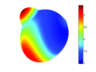
Refer to caption
(a) f2subscript𝑓2f_{2} with f2C(𝕊2)3.41subscriptnormsubscript𝑓2𝐶superscript𝕊23.41\|f_{2}\|_{C(\mathbb{S}^{2})}\approx 3.41
Refer to caption
(b) f2δsuperscriptsubscript𝑓2𝛿f_{2}^{\delta} with δ=0.5𝛿0.5\delta=0.5
Refer to caption
(c) l2l1subscript𝑙2subscript𝑙1l_{2}-l_{1} restoration with pL,NC(𝕊2)3.30subscriptnormsubscript𝑝𝐿𝑁𝐶superscript𝕊23.30\|p_{L,N}\|_{C(\mathbb{S}^{2})}\approx 3.30
Refer to caption
(d) l2l2subscript𝑙2subscript𝑙2l_{2}-l_{2} restoration with pL,NC(𝕊2)3.62subscriptnormsubscript𝑝𝐿𝑁𝐶superscript𝕊23.62\|p_{L,N}\|_{C(\mathbb{S}^{2})}\approx 3.62
Refer to caption
(e) l2l1subscript𝑙2subscript𝑙1l_{2}-l_{1} restoration errors
Refer to caption
(f) l2l2subscript𝑙2subscript𝑙2l_{2}-l_{2} restoration errors
Figure 5: Restoration of f2subscript𝑓2f_{2} using spherical 370.1subscript370.137_{0.1}-design with models (58) and (59)

A spherical 370.1subscript370.137_{0.1}-design with 514 points is used as the data point set in this experiment. Other settings in this experiment are δ=0.5𝛿0.5\delta=0.5, λ=1020,1019.5,,105𝜆superscript1020superscript1019.5superscript105\lambda=10^{-20},10^{-19.5},\ldots,10^{5}, 𝐱c=(0.5,0.5,0.5)Tsubscript𝐱𝑐superscript0.50.50.5𝑇\mathbf{x}_{c}=(-0.5,-0.5,\sqrt{0.5})^{T}, r=0.5𝑟0.5r=0.5 and ρ=1𝜌1\rho=1. The restorations of f2subscript𝑓2f_{2} using both models (58) and (59) are depicted in Fig. 5.3. Similar with previous experiments, we choose the values of λ𝜆\lambda resulting in minimal uniform errors for each model and plot the shape of the restoration function on the sphere. From Fig. 5.3(c)(d)(e)(f), restoration by model (58) is not as smooth as restoration by model (59) but has smaller errors. And more notably, as highlighted by the rectangle in Fig. 5.3(c)(d), model (58) restores the non-smooth edges of the spherical cap more accurately than model (59).

Acknowledgement. We would like to thank Professor Ian Sloan for his valuable and helpful comments on spherical tϵsubscript𝑡italic-ϵt_{\epsilon}-designs.

References

  • [1] M. Abramowitz and I. A. Stegun, Handbook of mathematical functions, vol. 1, Dover New York, 1972.
  • [2] C. An, X. Chen, I. H. Sloan, and R. S. Womersley, Well conditioned spherical designs for integration and interpolation on the two-sphere, SIAM J. Numer. Anal., 48 (2010), pp. 2135–2157.
  • [3]  , Regularized least squares approximations on the sphere using spherical designs, SIAM J. Numer. Anal., 50 (2012), pp. 1513–1534.
  • [4] K. Atkinson and W. Han, Spherical harmonics and approximations on the unit sphere: an introduction, Springer, 2012.
  • [5] B. Bajnok, Construction of spherical t-designs, Geom. Dedicata, 43 (1992), pp. 167–179.
  • [6] E. Bannai, On tight spherical designs, J. Comb. Theory Ser. A, 26 (1979), pp. 38–47.
  • [7] E. Bannai and E. Bannai, A survey on spherical designs and algebraic combinatorics on spheres, European J. Combin., 30 (2009), pp. 1392–1425.
  • [8]  , Remarks on the concepts of t-designs, J. Appl. Math. Comput., 40 (2012), pp. 195–207.
  • [9] B. J. C. Baxter and S. Hubbert, Radial basis functions for the sphere, in Recent Progress in Multivariate Approximation, Springer, 2001, pp. 33–47.
  • [10] A. Bondarenko, D. Radchenko, and M. Viazovska, Optimal asymptotic bounds for spherical designs, Ann. Math., 178 (2013), pp. 443–452.
  • [11] P. Borwein, Polynomials and polynomial inequalities, Springer, 1995.
  • [12] J. Brauchart, E. Saff, I. Sloan, and R. Womersley, Qmc designs: optimal order quasi monte carlo integration schemes on the sphere, Math. Comp., 83 (2014), pp. 2821–2851.
  • [13] J. S. Brauchart and K. Hesse, Numerical integration over spheres of arbitrary dimension, Constru. Approx., 25 (2007), pp. 41–71.
  • [14] X. Chen, S. Du, and Y. Zhou, A smoothing trust region filter algorithm for nonsmooth nonconvex least squares problems, tech. report, SIAM Annual Meeting 2014, Chicago, July, 7–11 2014.
  • [15] X. Chen, A. Frommer, and B. Lang, Computational existence proofs for spherical t-designs, Numer. Math., 117 (2011), pp. 289–305.
  • [16] F. H. Clarke, Optimization and nonsmooth analysis, vol. 5, SIAM, 1990.
  • [17] P. Delsarte, J. Goethals, and J. J. Seidel, Spherical codes and designs, Geometriae Dedicata, 6 (1977), pp. 363–388.
  • [18] M. Gräf and D. Potts, On the computation of spherical designs by a new optimization approach based on fast spherical fourier transforms, Numer. Math., 119 (2011), pp. 699–724.
  • [19] R. H. Hardin and N. J. Sloane, Mclaren s improved snub cube and other new spherical designs in three dimensions, Discrete Comput. Geom., 15 (1996), pp. 429–441.
  • [20] K. Hesse and I. H. Sloan, Worst-case errors in a sobolev space setting for cubature over the sphere s2superscript𝑠2s^{2}, Bull. Austr. Math. Soci., 71 (2005), pp. 81–105.
  • [21]  , Cubature over the sphere 𝕊2superscript𝕊2\mathbb{S}^{2} in sobolev spaces of arbitrary order, J. Approx. Theory, 141 (2006), pp. 118–133.
  • [22] J. Korevaar and J. L. H. Meyers, Spherical faraday cage for the case of equal point charges and chebyshev-type quadrature on the sphere, Intger. Transf. Spec. F., 1 (1993), pp. 105–117.
  • [23] S. V. Pereverzyev, I. H. Sloan, and P. Tkachenko, Parameter choice strategies for least-squares approximation of noisy smooth functions on the sphere, RICAM Report, 5 (2014).
  • [24] R. J. Renka, Multivariate interpolation of large sets of scattered data, ACM Trans. Math. Softw. (TOMS), 14 (1988), pp. 139–148.
  • [25] E. B. Saff and A. B. J. Kuijlaars, Distributing many points on a sphere, Math. Intell., 19 (1997), pp. 5–11.
  • [26] P. D. Seymour and T. Zaslavsky, Averaging sets: a generalization of mean values and spherical designs, Adv. Math., 52 (1984), pp. 213–240.
  • [27] I. H. Sloan and R. S. Womersley, A variational characterisation of spherical designs, J. Approx. Theory., 159 (2009), pp. 308–318.
  • [28]  , Filtered hyperinterpolation: a constructive polynomial approximation on the sphere, GEM-Intern. J. Geomath., 3 (2012), pp. 95–117.
  • [29] J. Sun and G. W. Stewart, Matrix Perturbation Theory, Computer Science and Scientific Computing, Academic Press, 1990.
  • [30] D. S. Watkins, Fundamentals of Matrix Computations, vol. 64, John Wiley & Sons, 2004.
  • [31] H. Wendland, Scattered Data Approximation, vol. 17, Cambridge University Press, 2005.