Uniform framework for the recurrence-network analysis of chaotic time series

Abstract

We propose a general method for the construction and analysis of unweighted $\epsilon$ - recurrence networks from chaotic time series. The selection of the critical threshold $\epsilon_{c}$ in our scheme is done empirically and we show that its value is closely linked to the embedding dimension $M$. In fact, we are able to identify a small critical range $\Delta\epsilon$ numerically that is approximately the same for the random and several standard chaotic time series for a fixed $M$. This provides us a uniform framework for the non subjective comparison of the statistical measures of the recurrence networks constructed from various chaotic attractors. We explicitly show that the degree distribution of the recurrence network constructed by our scheme is characteristic to the structure of the attractor and display statistical scale invariance with respect to increase in the number of nodes $N$. We also present two practical applications of the scheme, detection of transition between two dynamical regimes in a time delayed system and identification of the dimensionality of the underlying system from real world data with limited number of points, through recurrence network measures. The merits, limitations and the potential applications of the proposed method have also been highlighted.

I INTRODUCTION

Study of networks has become an important area of research in the last two decades cutting across various disciplines and often providing a coherent view of structures and phenomena which may appear different from a common perspective. Mathematically, networks are entities defined on an abstract space, with $N$ number of nodes and arbitrary number of links between them. We often refer to complex networks, implying that the structure is irregular and complex. Such networks may be weighted or unweighted, directed or undirected depending on the structure and interaction of the system it tries to model.

Historically, the study of networks has been the domain of a branch of mathematics called graph theory. The mathematical basis for the analysis of complex networks was laid using the so called “random graphs”(RG) by Erdős and Rényi about five decades back erd . They have shown several properties for random graphs, which are now popularly known as Erdős-Rényi (E-R) networks. The measures introduced for the analysis of RGs have, naturally, become the tools to characterize the structure and evolution of complex networks. The most important among them are the degree distribution and the characteristic path length (CPL), apart from other measures, such as, link density (LD), clustering coefficient (CC), diameter, centrality, etc. The degree distribution indicates how many nodes $n_{k}$ among the total number of nodes $N$ have a given degree $k$. It is usually represented as a probability distribution $P(k)$ as a function of $k$, where $P(k)={{n_{k}}\over{N}}$. For E-R networks, one can show that $P(k)$ follows a Binomial distribution which, for large $N$ and small probability of connection tends to the Poisson distribution. The CPL, denoted by $<l>$, is defined through the shortest path $l_{s}$ connecting two nodes $\imath$ and $\jmath$. For unweighted and undirected networks that we consider in this work, $l_{s}$ is defined as the minimum number of nodes to be traversed to reach from $\imath$ to $\jmath$. The average value of $l_{s}$ for all the pair of nodes in the whole network is defined as $<l>$ and the maximum value of $l_{s}$ is taken as the diameter of the network, denoted by $l_{D}$. For a detailed discussion of all the network measures, see the popular books by Newman new1 and Watts wat1 and some excellent reviews on the subject alb1 ; boc .

An important area where the new network based concepts and measures have been applied successfully is in the analysis of dynamical systems str1 ; barz , especially those showing chaotic behavior, by constructing complex networks from time series data of the dynamical systems. Here, the aim is to extract information regarding the structure of the underlying chaotic attractor, which are otherwise difficult to get using the conventional methods of nonlinear time series analysis. The basic idea of this technique is that the information inherent in a chaotic time series is mapped on to the domain of a complex network using a suitable scheme. One then uses the statistical measures of the complex network to characterize the underlying chaotic attractor.

Two questions are relevant in this context. Firstly, which method is to be used to transform the time series into the corresponding network and secondly, how to ensure that the resulting network truly represents the characteristic features of the underlying attractor. To answer the first, several methods have been suggested in the literature, such as cycle networks zha1 , visibility graphs lac , transition networks nic and recurrence networks (RN) mar1 . The RNs can be constructed in different ways, namely, the correlation networks yan1 , $k$-nearest neighbour networks xu1 and $\epsilon$-recurrence networks don1 . It has been shown that the networks generated by each of these methods can capture several characteristics of the chaotic time series like dynamical transitions in the system, topological properties of the attractor, etc. Hence each method is relevant in the context of specific applications. A detailed discussion of these methods and their comparison can be found elsewhere don2 ; don3 .

Among the methods mentioned above, the one based on $\epsilon$ - recurrence is physically appealing since it is based on the concept of recurrence of a trajectory in the phase space. Moreover, the method can be applied to any type of synthetic or real world data and the resulting networks are found to be useful tools for uncovering complex bifurcation scenario and detecting dynamical transitions in palaeo-climate data zou1 ; dong1 ; gao1 . The methods based on recurrence have also found diverse applications ranging from life sciences wes1 ; ram1 , earth sciences tra1 and astrophysics zol . In this work, we concentrate on this method for network generation, confining ourselves to the case of unweighted $\epsilon$-recurrence networks.

The answer to the second question raised above leads us to the choice of the parameters for network construction. A crucial parameter in the construction of the RN is the recurrence threshold $\epsilon$ itself. In all the existing schemes, the value of $\epsilon$ chosen is different for each time series, whatever be the criteria used for its selection, due to the arbitrary size of the attractor after embedding. Our main goal in the present work is to propose a scheme that uses an approximately identical range of values for $\epsilon$ for different time series, both synthetic and real world, for a given embedding dimension. Apart from providing a uniform framework for the recurrence network analysis, the scheme has several advantages and practical applications as discussed below in detail.

Our paper is organised as follows: In the next section, we discuss the basic idea of RN construction while in §III, the criteria for the selection of all the parameters for the construction of RN from the time series are presented. We then proceed, in §IV, to construct the RNs from several low dimensional chaotic systems. All the important network measures are derived from the RNs as a function of $M$ and $N$ and compared. The degree distribution, especially, is studied in detail and is shown to be characteristic of the structural complexity of a chaotic attractor. Two practical applications of the proposed scheme are illustrated in §V. A discussion on various aspects of implementation of the scheme and conclusions are given in §VI.

II CONSTRUCTION OF RECURRENCE NETWORK

In this section, we briefly discuss the basic idea regarding the construction of recurrence networks. More details can be found in recent reviews on the topic don2 ; don3 . Recurrence is a fundamental property of every bounded dynamical system by which a trajectory tends to revisit a certain region of the phase space over a time interval. This basic concept has been utilized to develop a visualization tool called the recurrence plot (RP) for the analysis of dynamical systems eck . A RP represents all recurrences in the form of a binary matrix $\mathcal{R}$ where $R_{ij}$ = 1 if the state $\vec{x_{j}}$ is a neighbour of $\vec{x_{i}}$ in phase space and $R_{ij}=0$, otherwise. The neighbourhood is defined through a certain recurrence threshold $\epsilon$. In the most general definition, the discretely sampled scalar time series $s(1),s(2),.....s(N_{T})$ is embedded in $M$-dimensional space taking the time delay co-ordinates gra using a suitable time delay $\tau$, where $N_{T}$ is the total number of points in the time series. The procedure creates delay vectors in the embedded space of dimension $M$ given by

$$\vec{x_{i}}=[s(i),s(i+\tau),......s(i+(M-1)\tau)]$$ (1)

There are a total number of $N=N_{T}-(M-1)\tau$ state vectors in the reconstructed space representing the attractor. Any point $\jmath$ on the attractor is considered to be in the neighbourhood of a reference point $\imath$ if their distance in the $M$-dimensional space is less than the threshold $\epsilon$. Thus we have

$$R_{ij}=H(\epsilon-||\vec{x_{i}}-\vec{x_{j}}||)$$ (2)

where $H$ is the Heaviside function and $||..||$ is a suitable norm. In this paper, we use the Euclidean norm. The RP can only visually distinguish between different qualitative features of dynamics. This tool has become more popular with the introduction of the recurrence quantification analysis (RQA) mar2 using the measures derived from the RP. It has found numerous applications giu ; fac ; lit and even dynamical invariants like correlation dimension $D_{2}$ and correlation entropy $K_{2}$ can be evaluated efficiently using RQA thi .

The importance of the $\epsilon$ - RN (which, from now on, we simply call RN) is that its generation is closely associated with the RP. In fact, the adjacency matrix $\mathcal{A}$ for the unweighted RN can be obtained by removing the identity matrix from the recurrence matrix:

$$A_{ij}=R_{ij}-\delta_{ij}$$ (3)

where $\delta_{ij}$ is the Kronecker delta. Note that, once the adjacency matrix is defined, the time series has been converted into a complex network. Each point on the embedded attractor is taken as a node in the RN and a node $\imath$ is connected to another node $\jmath$ if the distance $d_{ij}$ between the corresponding points on the embedded attractor is $\leq\epsilon$. Thus the adjacency matrix $\mathcal{A}$ is a binary symmetric matrix with elements $A_{ij}=1$ if ${d_{ij}\leq\epsilon}$ and $0$ otherwise. Note that, in contrast to the RP measures which consider the temporal properties of the trajectory points, RN analysis quantifies the geometrical properties of the underlying attractor and hence can give useful information regarding the structure of the attractor.

Even though the method for the generation of the RN appears to be simple, it has several ambiguities associated with it don4 . How do we ensure that the RN captures the structural characteristics of the underlying attractor? The answer lies in the proper choice of the parameters involved in the construction of the network. For the RN, the key parameters are $\epsilon$ and $M$. If $\epsilon$ is large, specific small scale properties of the attractor cannot be revealed and if $\epsilon$ is too small, the network breaks into dissuaded nodes due to lack of connections. Many authors dong1 ; gao2 ; sch ; dong2 have discussed this issue in detail and have given some guidelines for the choice of $\epsilon$. But for arbitrary size of the attractor, the choice of $\epsilon$ still remains subjective. Similarly, the specific feature of RN generation is embedding and in this context the choice of $M$ has not been discussed much in the literature as it is commonly believed that $M$ should be sufficiently high for the attractor to be fully resolved. We show that the choice of $\epsilon$ is closely related to that of $M$ and we present a scheme for the choice of $\epsilon$ and $M$ that gives a uniform critical range of $\epsilon$ for all time series for a given $M$. To validate the wide range of applicability of the scheme, we show results from several low dimensional chaotic attractors as well as random data.

III CHOICE OF PARAMETERS FOR NETWORK CONSTRUCTION

There are four parameters associated with the RN generation, which are the time delay $\tau$, $\epsilon$, $M$ and $N$, the number of nodes. Note that $N<N_{T}$, the total number of points in the time series and the difference depends on $M$ and $\tau$. The value of $N_{T}$ can be adjusted to get the required number of $N$ for the computation. For the choice of $\tau$ we stick to the most commonly used criteria, namely, the first minimum of the autocorrelation function. The value of $\tau$ is related to the time step $\Delta t$ used for the generation of the time series. For the sake of uniformity, we use $\Delta t=0.05$ to generate the time series from all the continuous time systems presented here. We have removed the first $10000$ values as transients in all cases.

In all our numerical computations we use the value of $N$ in the range $2000$ to $10000$. The lower limit is set because, if the number of data points in the time series is too small, the basic structure of the embedded attractor may not have evolved completely. The upper limit is set mainly due to the fact that the computations become increasingly difficult due to high memory requirement for $N>10000$. However, we find that $N<10000$ is sufficient to get reasonable results from low dimensional chaotic systems. Moreover, for many real world applications of RN analysis, one has to confine to this range of $N$ very often.

We next consider the choice of the crucial parameter, namely, the critical threshold, $\epsilon_{c}$. There are already a number of criteria suggested for choosing $\epsilon_{c}$. For example, Gao and Jin gao2 gives a heuristic criterion that selects $\epsilon_{c}$ as the value at which the link density becomes maximum when plotted as a function of $\epsilon$. But this has the drawback that small changes in $\epsilon$ induce large changes in the network measures as indicated by Donner et al. don4 . Recently, another criterion has been suggested based on analytic methods dong2 while an adaptive selection of threshold has been proposed by Eroglu et al. for specific time series ero1 . The last one is especially important as it chooses the critical threshold based on the theory of random graphs, where the second smallest eigen value $\lambda_{2}$ of the Laplacian matrix $\mathcal{L}$ crosses zero when plotted as a function of $\epsilon$ as the network becomes fully connected boc , where $\mathcal{L}=\mathcal{D}-\mathcal{A}$, the difference between diagonal degree matrix and adjacency matrix. We will show below that this criterion comes very close to the empirical criterion used by us.

In all the above works so far considered, the size of the attractor after embedding is arbitrary so that the value of the threshold will be different for different attractors. Our primary motivation in the present work is to look for a scheme that can give approximately identical value for the critical threshold for different time series. We consider this to be an important step forward as it will lead to a uniform framework for the RN analysis which may be more useful for application to practical time series, as shown below.

To overcome the problem of arbitrary size of the attractor, we transform the time series into a uniform deviate. For this, we first rescale the time series into the unit interval $[0,1]$. We then take each value $y_{i}$ in the time series and count how many values are less than or equal to $y_{i}$. Let this count be $n_{i}$. Then the uniform deviate time series $u_{i}$ is obtained as $u_{i}={{n_{i}}\over N_{T}}$ where $N_{T}$ is the total number of points in the time series. The effect of uniform deviate transformation is shown in Fig. 1 for the Lorenz attractor, where the original time series $y(t)$ and the time series after uniform deviate $u(t)$ are shown along with the corresponding attractors after embedding. We have shown the importance of uniform deviate transformation in computing the conventional nonlinear measures like correlation dimension $D_{2}$ and entropy $K_{2}$ kph1 ; kph2 , especially from higher dimensional systems kph3 . It stretches the embedded attractor uniformly in all directions without changing any of the dynamical invariants of the attractor, minimises the edge effect and provides improved scaling region and better convergence with data points.

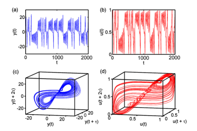
Figure 1: (Color online) Top panel shows the original time series $y(t)$ from the Lorenz attractor on the left and the time series $u(t)$ after uniform deviate transformation on the right. The bottom panel shows the corresponding attractors after embedding.

The primary criterion that we use for the selection of $\epsilon_{c}$ in our scheme is that the resulting RN has to remain mostly as “one single cluster”. This is checked empirically by changing $\epsilon$. Note that this criterion is analogous to the one suggested by Donges et al. dong2 where the authors propose to choose the percolation threshold above which the giant component of the RN appears. For the selection of $\epsilon_{c}$, we use a more practical approach rather than the rigorous criterion as adopted by the previously mentioned authors and we show the advantages of our approach in the sections below. A formal method to select $\epsilon_{c}$ is to choose the value of $\epsilon$ when the network just becomes fully connected. This is done by computing the second smallest eigen value $\lambda_{2}$ of the Laplacian matrix as a function of $\epsilon$. From the theory of random graphs, it is well known boc that as $\lambda_{2}$ crosses zero from negative, the network becomes fully connected, with no dissuaded nodes. In Fig. 2, we show the variation of $\lambda_{2}$ with $\epsilon$ for RNs constructed from Lorenz and random time series, for $N=2000$ and $5000$, with $M=3$. It is evident that $\lambda_{2}$ for random network becomes positive slightly earlier compared to Lorenz in both cases. As $N$ increases, there is also a slight shift towards lower $\epsilon$. The network for random becomes fully connected for $\epsilon=0.09$ while for Lorenz, the value is $0.13$. We have repeated the computation for other standard chaotic attractors and found that the value of $\epsilon$ where $\lambda_{2}$ becomes positive varies slightly for different systems. However, we find that there is a small range of $\epsilon$, from $0.1$ to $0.13$, where the network is almost fully connected for all systems with the appearance of a giant cluster and very few $(<1\%)$ dissuaded nodes. This range is found to be common for all the systems we have analysed for a fixed $M$. Thus, the primary criterion provides a small uniform range of $\epsilon$ for many standard chaotic systems.

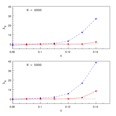
Figure 2: (Color online) Variation of the second smallest eigen value $\lambda_{2}$ of the Laplacian matrix as a function of $\epsilon$ for the RNs from Lorenz (filled circles connected by red solid line) and random (filled triangles connected by blue dashed line) time series. Results are shown for RNs with $N=2000$ and $5000$, constructed with $M=3$. The dotted line is a reference for zero.

In order to ensure that the RN is a true representation of the chaotic attractor, we apply an additional constraint that RN measures from standard chaotic time series are significantly different from that of a random time series. Though this condition appears to be subjective, we show below that it gives consistent results for all the standard chaotic systems considered in this work. For this, we compute the three important network measures, LD, CC and CPL for the RN from some standard chaotic times series as a function of $\epsilon$ and compare them with the corresponding measures from the RN of random time series. The equations for computing these measures are discussed in detail in the next section. We then find that the measure CPL is a good candidate to apply this additional constraint. This is shown in Fig. 3 for two standard chaotic time series. For $\epsilon$ below $0.1$, there are multiple disconnected networks with no giant cluster and the CPL computed is for the largest component. It is evident from the figure that there is a small range of $\epsilon$, say $\Delta\epsilon$, (marked by the two vertical dashed lines) where the difference in the value of CPL of the RN from chaotic time series and that of random is maximum and as $\epsilon$ increases above this range, the CPL for RN from all chaotic time series approaches that of random time series. More importantly, this range, which we call the critical range, is found to be approximately identical for all the systems we have analysed and coincides with the common range found above corresponding to the emergence of the giant component in the RN. However, it should be emphasized that this range, $\Delta\epsilon$, is an empirical result and hence it is difficult to set any specific criterion for the upper bound either in terms of $M$ or $N$. We choose the minimum value of this range as the critical threshold $\epsilon_{c}$, for the construction of RN which we believe will capture the characteristic properties of the attractor. Nevertheless, we have checked and confirmed that any $\epsilon$ within $\Delta\epsilon$ does not make any qualitative change in the degree distribution of the RN and the related network measures to be presented below. Note that we do not follow the condition $\lambda_{2}>0$ strictly as chosen by Eroglu et al. ero1 , as this makes $\epsilon_{c}$ slightly different for different RNs. We have constructed the RN using the Gephi software (https://gephi.org/) taking time series from several standard chaotic attractors for $\epsilon$ ranging from $0.05$ to $0.25$, taking $M=3$. We find that there is no giant cluster for $\epsilon<0.1$ while the network becomes over connected for $\epsilon>0.15$, in all cases.

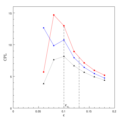
Figure 3: (Color online) Characteristic path length as a function of threshold for RNs generated from Lorenz (filled circles connected by red solid line at the top), Rössler (filled squares connected by blue solid line in the middle) and random (filled triangles connected by dotted line) time series with $N=2000$ and $M=3$. The two vertical dashed lines indicate the critical range of $\epsilon$ where CPL from chaotic time series differs from that of random time series. The critical threshold $\epsilon_{c}$ is the minimum of this range. Below $\epsilon_{c}$, there is no giant cluster.

We now consider how the value of $\epsilon_{c}$ changes with $M$ and $N$. To study this, we generate RNs from a number of low dimensional chaotic systems, both discrete and continuous, by varying $N$ from $2000$ to $10000$ and $M$ from $2$ to $5$. For each $N$ and $M$, we scan a range of $\epsilon$ values between $0.02$ to $0.20$. The results from this detailed numerical analysis are compiled in Fig. 4 separately for continuous and discrete systems. The variation of $<l>$ corresponding to $\Delta\epsilon$ as $N$ and $M$ changes is shown with that of random time series as reference. The left panel shows the dependence on $N$ and the right panel shows the dependence on $M$. To study the dependence on $N$, we use the natural dimension of the system, namely, $M=3$ for continuous systems (top) and $M=2$ for discrete systems (bottom). Note that $\Delta\epsilon$ for $M=2$ has been shifted to $0.06-0.08$. Moreover, in both cases, ($M=2$ and $3$), there is only a small decrease in $\Delta\epsilon$ as $N$ is increased from $2000$ to $10000$. This means that one can effectively use the same $\epsilon$ for this whole range of $N$ values.

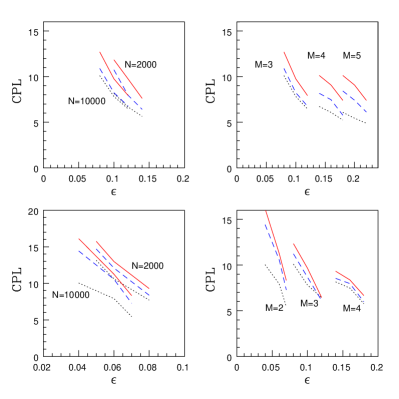
Figure 4: (Color online) The figure shows how the critical range $\Delta\epsilon$ (see text) varies with respect to $N$ and $M$. The left panel shows $\Delta\epsilon$ for two values of $N$ as indicated, where the top panel is for continuous systems with $M=3$ and the bottom panel for discrete systems with $M=2$. The right panel shows the variation of $\Delta\epsilon$ with $M$ for $N$ fixed at $10000$. In the top panel, the red solid line is for Lorenz attractor and the blue dashed line is for Rössler attractor, while in the bottom panel, the same is for Lozi and Henon attractors respectively. In all figures, the dotted line is for random time series.

In the right panel, we show the effect of increasing the embedding dimension from the natural dimension of the system, with $N$ fixed as $10000$. Note that the value of $\epsilon_{c}$ clearly shifts with $M$ which implies that each $M$ requires a corresponding $\epsilon_{c}$ for the generation of the RN. But the more interesting result is that, for all the systems that we have analysed, we are able to find approximately the same critical range $\Delta\epsilon$ corresponding to each $M$. This range is given in Table 1 where, $\epsilon_{c}$ in the third column is the critical threshold used by us corresponding to each $M$ for all the further computations in this paper. Thus, even though our criterion for the selection of $\epsilon_{c}$ is not completely novel, we are able to provide a certain level of non-subjectivity in its choice which, we hope, will make the application of RN analysis more effective.

It may be noted that the above choice of the critical range of $\epsilon$ is, in fact, analogous to and motivated by the selection of a scaling region in the conventional nonlinear time series analysis for deriving dynamical invariants like $D_{2}$. We have already shown that the scaling region for many low dimensional chaotic systems can be selected algorithmically for a non-subjective computation of $D_{2}$ and $K_{2}$ kph1 ; kph4 . It is well known that the choice of the scaling region critically depends on the embedding dimension $M$, while the change is not much if the number of data points changes from $2000$ to $10000$. In this way, the above result of getting an approximately same range of $\Delta\epsilon$ for different chaotic systems is not very surprising.

M	Critical Range of $\epsilon$	$\epsilon_{c}$
2	0.06 - 0.08	0.06
3	0.10 - 0.13	0.10
4	0.14 - 0.18	0.14
5	0.18 - 0.22	0.18

Table 1: Critical range of $\epsilon$ obtained empirically for each value of $M$

We now give a simple mathematical explanation for the observed numerical results regarding the relation between $\epsilon$ and $M$. Consider a random distribution of $N$ points in $M$ dimension. After uniform deviate transformation, the volume of the embedding space is unity and the average density of points $<\rho>=N$. The average separation between two points along any direction is

$$<d>\sim({{1}\over{N}})^{1/M}\sim({{1}\over{<\rho>}})^{1/M}$$ (4)

This gives the critical value of distance for a given $M$ below which the degree of a node tends to zero on the average. Hence $\epsilon_{c}$ for the random RN for each $M$ must be sufficiently greater than $<d>$.

To get more insight on the result given in Table 1 and know how $\epsilon_{c}$ varies for higher $M$ values, we consider the limiting value of $\epsilon$, say $\epsilon_{f}$, at which the RN is fully connected. That is, every node is connected to every other node with the degree of each node $(N-1)$ and the LD reaches its maximum possible value $1$. Since we consider a uniform deviate, the size of the attractor is unity. For $M=2$, the value of $\epsilon$ at which this happens is the diagonal length of the square, that is, $\epsilon_{f}(2)\equiv\sqrt{2}$. For $M=3$, $\epsilon_{f}(3)$ increases to $\sqrt{3}$ and one can easily show that, in general, $\epsilon_{f}(M)\equiv\sqrt{M}$. Note that this result is independent of $N$. This also implies that the difference between successive $\epsilon_{f}$, $\epsilon_{f}(M)-\epsilon_{f}(M-1)$, slowly decreases with $M$. Since the LD corresponding to $\epsilon_{c}$ is effectively a fraction of the total LD, one expects roughly the same dependence for $\epsilon_{c}$ on $M$, that is $\epsilon_{c}\propto\sqrt{M}$. We have numerically verified this for the random RN for $M$ upto $7$. This means that, though the difference between successive $\epsilon_{c}$ appears to be almost a constant for small $M$ as given in Table 1, this difference decreases slowly as $M$ increases.

As a final test to validate our choice of $\epsilon_{c}$, we undertake a counter check by computing $D_{2}$ of some standard chaotic attractors using the RP (which is equivalent to the adjacency matrix) corresponding to $\epsilon_{c}$. The method proposed by Thiel et al. thi is used for this purpose. This method uses the cumulative probability distribution $p^{c}(l)$ of the diagonal lines in the RP, corresponding to two different thresholds $\epsilon$ and $\epsilon+\Delta\epsilon$ using the relation:

$$D_{2}(\epsilon)={{log[{{p^{c}(\epsilon,l)}\over{p^{c}(\epsilon+\Delta\epsilon,l)}}]}\over{log[{{\epsilon}\over{\epsilon+\Delta\epsilon}}]}}$$ (5)

We have found that the $D_{2}$ values obtained in all cases are closer to the standard values for $\epsilon=\epsilon_{c}$. This implies that the geometric complexity of the attractor is truly reflected in the RN constructed by our scheme.

IV MEASURES FROM RECURRENCE NETWORK

We now compute the important network measures from the RN of several low dimensional chaotic attractors, including discrete systems (maps) in two dimensions and continuous systems (flows) in three dimensions. For all systems, $M$ is varied from 2 to 5 using the $\epsilon_{c}$ corresponding to each $M$ with $N$ varied from $2000$ to $10000$.

IV.1 Characteristic Path Length, Clustering Coefficient and Link Density

We first compute the CPL, CC and LD from the RN and study their dependence on $N$ and $M$. The equations for computing these measures have been discussed in detail in the literature new1 ; alb1 . The CPL is given by the equation

$$<l>={{1}\over{N(N-1)}}\sum_{i,j}^{N}l_{s}$$ (6)

where $l_{s}$ is the shortest path length for all pair of nodes $(\imath,\jmath)$ in the network. The maximum value of $l_{s}$ is taken as the diameter of the network, $l_{D}$. If $k_{i}$ is the degree of the $\imath^{th}$ node, then

$$LD={{1}\over{N(N-1)}}\sum_{i}^{N}k_{i}$$ (7)

The CC of the network is defined through a local clustering index $c_{v}$. Its value is obtained by counting the actual number of edges in a sub graph with respect to node $v$ as reference to the maximum possible edges in the sub graph:

$$c_{v}={{\sum_{i,j}A_{vi}A_{ij}A_{jv}}\over{k_{v}(k_{v}-1)}}$$ (8)

The average value of $c_{v}$ is taken as the CC of the whole network:

$$CC={{1}\over{N}}\sum_{v}c_{v}$$ (9)

In Fig. 5 top panel, we show the variation of $<l>$ with $N$ for two standard chaotic systems for $M=3$. RN from random time series is also added for comparison. Note that in all cases, $<l>$ initially decreases with $N$, but saturates as $N\rightarrow 10000$, with the value of $<l>$ for RN from random time series always less compared to that from chaotic systems. The variation of $<l>$ with $N$ can be understood from the degree distribution of the RN discussed in detail in the next section. We find that as $N$ increases, the average degree of the nodes $<k>$ also increases correspondingly. Typically, as $N$ increases to $2N$, $<k>$ shifts approximately to $<2k>$, reducing $<l>$. In the bottom panel, we show the variation of CC with $N$ which is found to be approximately constant for all systems for the range of $N$ used.

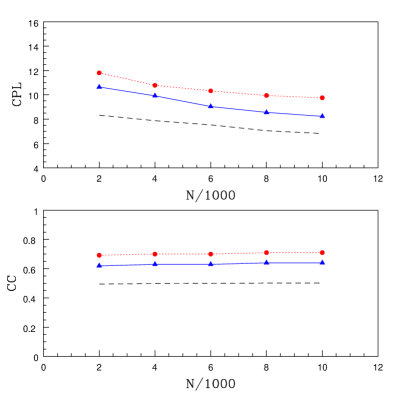
Figure 5: (Color online)Variation of CPL (top panel) and CC (bottom panel) with $N$ for RNs generated from Lorenz (filled circles connected dotted line), Rössler (filled triangles connected by solid line) and random (dashed line) time series. The value of $M$ is fixed as $3$.

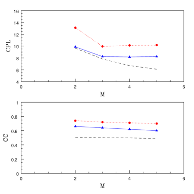
Figure 6: (Color online)Same as the previous figure, but the variation is with respect to $M$ for a fixed $N=10000$. Note that CPL saturates at the natural dimension of the system.

We have also studied numerically the variation of $<l>$ and CC with $M$ by fixing $N=10000$ and the results for the same two systems are shown in Fig. 6. While CC remains constant, the variation of $<l>$ is more interesting, showing saturation for $M$ equal to or greater than the actual dimension of the system. We will show below that the same is true for degree distribution as well, leading to an important practical application of network measures.

IV.2 Degree Distribution

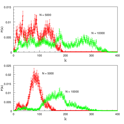
Figure 7: (Color online) Degree distribution of the RN generated from the Lorenz attractor (top panel) for $N=5000$ (open red circles) and $N=10000$ (filled green triangles appearing in light gray shade in print), as indicated. Corresponding results for Rössler attractor are shown in the bottom panel. In both cases, we use $M=3$ and $\epsilon_{c}=0.1$.

We now consider the most important measure of a network, namely, the degree distribution $P(k)$ versus $k$. In Fig. 7, we show the degree distribution of the RN from Lorenz and Rössler attractor time series for $N=5000$ and $10000$ by using $M=3$ and $\epsilon=0.1$. Note that the error bar is estimated from counting statistics resulting from the finiteness in the number of nodes. The statistical error associated with any counting of $n(k)$ is $\sqrt{n(k)}$. If $n(k)\rightarrow 0$, one typically takes the error to be normalised as 1. Thus, the error associated with $P(k)$ is typically ${{\sqrt{n(k)}}\over{N}}$ and becomes $1/N$ as $n(k)\rightarrow 0$. It is evident from the figure that as $N$ is doubled, the degree $k$ of each node gets approximately doubled resulting in a shift along the X-axis and the range $[k_{min},k_{max}]$ of $k$ values is shifted approximately to twice the range. Correspondingly, the $P(k)$ values are reduced since the area under the distribution curve is constant. Assuming that the $k$ values are continuous within the range $[k_{min},k_{max}]$, we can write

$$\sum_{k}\Delta kP(k)=1$$ (10)

where $\Delta k(\equiv 1)$ is the difference between successive $k$ values.

Changing $k$ to ${k^{{}^{\prime}}}\equiv{{k}\over{N}}$, $\Delta{k^{{}^{\prime}}}={{\Delta k}\over{N}}$ and $P(k)$ changes to $P(k^{{}^{\prime}})$ so that

$$\sum_{k^{{}^{\prime}}}\Delta k^{{}^{\prime}}P(k^{{}^{\prime}})=1$$ (11)

Substituting for $\Delta k$ in Eq.(10), we get

$$P(k^{{}^{\prime}})=NP(k)\equiv n(k)$$ (12)

It is convenient to represent the degree distribution in the rescaled variables as shown in Fig. 8. Note that the degree distribution for the two $N$ values have now become identical and can be considered as almost stationary in the rescaled variable $k/N$ apart from small statistical fluctuations. To capture the real trend in the distribution, we show in Fig. 9 the same distributions shown in the previous figure without error bar and the values connected by line.

One expects the scale invariance for the RN from a random time series whose degree distribution is Poissonian which can be approximated as Gaussian for large $N$. This is because, the degree of every node increases by an average value as $N$ increases and the degree distribution appears identical in the rescaled variable $k/N$ as can be seen from Fig. 10. Here we find that an arbitrary degree distribution from the RN of a chaotic attractor also shows this property. A possible explanation, for attractors whose measure is continuous is that, as the dynamical system evolves, the structure of the attractor also evolves in such a way that the probability density over the attractor is preserved once the basic structure of the attractor is formed. The degree $k_{i}$ of a reference node $\imath$ represents the local connectivity of the RN and it corresponds to the local phase space density around the reference point in the chaotic attractor from which the RN is constructed. It is well known that the local phase space density of the chaotic attractor is preserved in the RN don2 . Considering an infinitesimal hyper volume $V_{M}(\epsilon)$ in $M$-dimension with radius $\epsilon$ about a reference point $\vec{r}_{i}$ in phase space, one can write don2 :

$${{1}\over{N}}(k_{i}(\epsilon)+1)\approx\int_{V_{M}(\epsilon)}p(\vec{r})d^{M}\vec{r}\approx V_{M}(\epsilon)p(\vec{r}_{i})$$ (13)

where $p(\vec{r}_{i})$ is the invariant density around $\vec{r}_{i}$. Note that in LHS, $1$ is added to include the reference node (self loop). This gives a relation between the local measure in an attractor and that of a RN:

$$p(\vec{r}_{i})=\lim_{\epsilon\rightarrow 0}\lim_{N\rightarrow\infty}{{(k_{i}+1)}\over{V_{M}(\epsilon)N}}$$ (14)

The above equation tells us that for the RN constructed with $\epsilon_{c}$, the local probability density around a point on the attractor gets mapped to the degree of the corresponding node in the constructed RN. Since every point on the attractor is converted to a node on the RN, points with the same probability density will correspond to nodes with the same degree. The degree distribution tells how many nodes have a given degree in the RN. This is equivalent to finding how many local regions on the entire attractor have the same probability density. As we change from the phase space domain of the attractor to the domain of the network, the degree distribution represents the global statistical measure of the probability density variations over the entire attractor. Thus, it seems natural that the degree distribution of the RN from any chaotic attractor shows the scale invariance. The small deviations in the degree distribution as $N$ increases is the result of the corresponding small fluctuations in the probability density. Also, the range of $k$ values in the RN is a measure of the range of variation of $p(\vec{r})$ over the attractor. However, a direct relation connecting the probability distribution over the attractor and the degree distribution of the RN seems to be highly nontrivial owing to the fractal geometry of the attractor.

From the above discussion, it becomes clear that a peak at high $k$ value near $k_{max}$ in the degree distribution implies large number of relatively dense regions of high probability over the entire attractor. Many peaks in the degree distribution are indicative of large local density fluctuations over the attractor. For example, from Fig. 8 and Fig. 9, the fluctuation is much large for the RN from the Lorenz attractor compared to that of the Rössler attractor, though both have approximately the same range of $[k_{min},k_{max}]$. In this sense, one can say that the degree distribution is a characteristic measure of the structural complexity of an attractor. Note that this idea has been pointed out by many authors before don2 ; zou2 . Once the basic structure of the attractor is formed, a further increase in the number of nodes does not change the degree distribution qualitatively. In other words, RN analysis appears to be a useful tool to get meaningful results regarding structural and topological properties of the attractors with less number of data points. We now show that there is a part in the degree distribution that corresponds to the Poisson distribution where, the $k$ values occur more by chance than by choice.

For a random time series embedded in $M$-dimensional space, after being converted into uniform deviate, the average density of points $<\rho>=N$. Hence the average number of points inside a $M$-dimensional sphere of radius $\epsilon$ is $k_{ran}=NV_{M}$, where $V_{M}$ is the volume of the sphere. When the time series is converted into a RN, the condition for two nodes to be connected is that the distance is $<\epsilon$. In other words, for random RN, typically a node is connected to $k_{ran}$ other nodes. Or, most nodes will have degree $k_{ran}$ and the degree distribution tends to be a Poissonian around this value.

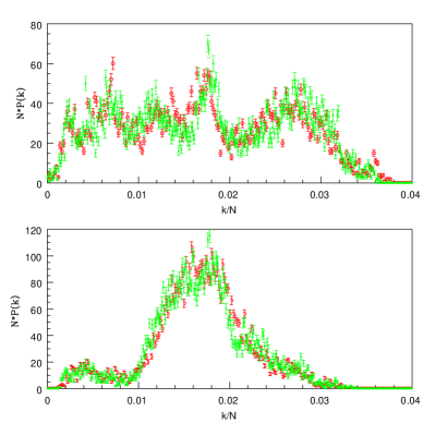
Figure 8: (Color online) Rescaled distributions (see text) of the Lorenz (top panel) and Rössler (bottom panel) attractors shown in the previous figure for $N=5000$ (open red circles) and $N=10000$ (filled green triangles appearing in light gray shade in print). Note that, after rescaling, the distributions for the two $N$ values become statistically identical in both cases.

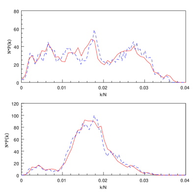
Figure 9: (Color online) The same distributions shown in the previous figure without error bar and connected by line, for clarity. The red solid line is for $N=5000$ and the blue dashed line is for $N=10000$.

Now, for a non random time series, there will be significantly more nodes with degree greater than $k_{ran}$ and it is these nodes which describe the structure of the underlying attractor. Nodes with degree $\sim k_{ran}$ occur more by chance association rather than the true description of the system. Thus, characteristic information regarding the system is given by the nodes with degree $>k_{ran}$ and hence the value of $k_{ran}$ should be small compared to the range of $k$ values in the degree distribution.

Note that the position of $k_{ran}$ in the degree distribution depends on the choice of $\epsilon$ and $M$. One expects a small peak around $k_{ran}$ in all degree distributions which becomes less significant as $N$ increases. We now estimate the value of $k_{ran}$ for the choice of $\epsilon$ and $M$ that we use to compute the degree distributions of chaotic attractors. For $M=3$, $V_{M}={{4}\over{3}}\pi\epsilon^{3}$ and hence

$$k_{ran}\approx N{{4}\over{3}}\pi\epsilon^{3}$$ (15)

With $\epsilon=0.1$, we get ${{k_{ran}}\over{N}}\approx 0.004$, which is independent of $N$. This is sufficiently small compared to the rescaled ${{k}\over{N}}$ values as can be seen from Fig. 8 and Fig. 9, where ${{k_{max}}\over{N}}\approx 0.04$. Since ${{k_{ran}}\over{N}}\propto\epsilon^{3}$ for $M=3$, a small increase in $\epsilon$ can shift the Poisson range significantly to the right in the degree distribution. This shows the importance of choosing the correct $\epsilon_{c}$.

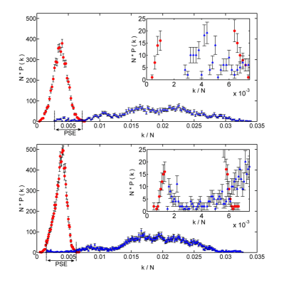
Figure 10: (Color online) Degree distribution of the RN from the Rössler attractor time series (filled blue triangles) in comparison with that of the random time series (filled red circles seen as Poisson distribution on the left). The top panel is for $N=5000$ and the bottom panel for $N=10000$, with $M=3$ and $\epsilon=0.1$ in both cases. We show the rescaled distributions so that both panels appear identical. The two vertical lines indicate the Poisson statistics part of the distribution or Poisson statistic error (denoted PSE) which coincides with the degree distribution of the random time series. It is shown magnified in the inset.

For the discrete systems with $M=2$, we have

$${{k_{ran}}\over{N}}\approx\pi\epsilon^{2}$$ (16)

Using the optimum value of $\epsilon=0.06$ used for $M=2$, we have ${{k_{ran}}\over{N}}\approx 0.011$ which is $<<{{k_{max}}\over{N}}$, as will be shown below for discrete systems. Finally, for $M=4$, we have a hyper cube of unit volume. The general formula for the volume of a Euclidean ball of radius $\epsilon$ in $M$-dimension (for even $M$) is:

$$V_{M}(\epsilon)={{\pi^{M/2}}\over{(\frac{M}{2})!}}\epsilon^{M}$$ (17)

For $M=4$, $V_{4}(\epsilon)={{\pi^{2}}\over{2}}\epsilon^{4}$. For the threshold $\epsilon=0.14$, we find ${{k_{ran}}\over{N}}\approx 0.00196$.

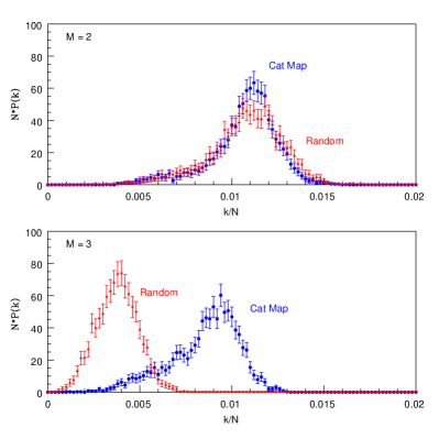
Figure 11: (Color online) Degree distributions of the RNs generated from Cat Map (filled blue circles) and random (filled red triangles) time series for $N=5000$ for two values of $M$, as indicated. Note that, in going from $M=2$ to $M=3$, the distribution of the random network is shifted while that for the Cat Map remains stationary.

The above results are explicitly shown in Fig. 10 and Fig. 11. In Fig. 10, we show the rescaled degree distributions of RNs from random and Rössler attractor time series plotted together for $N=5000$ and $10000$. Note that the Poisson distribution part, shown by the two vertical lines, almost exactly coincides with the degree distribution of the random time series. This part is shown magnified in the inset. In Fig. 11, we show the rescaled degree distributions of the Cat map and the random time series together for $M=2$ (top panel) and for $M=3$ (bottom panel). For $M=2$, both the distributions are almost identical and peak exactly at $k_{ran}=0.011$ in agreement with our calculations above. For $M=3$, the peak for the random distribution is shifted to $0.004$ as expected, while that for Cat map remains almost unchanged and hence both the distributions can be easily differentiated.

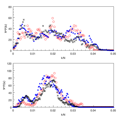
Figure 12: (Color online) Rescaled degree distributions (without error bar for clarity) for the RNs from Lorenz (top panel) and Rössler (bottom panel) attractor time series for $M=3$(open red circles), $M=4$(filled blue triangles) and $M=5$(black star like points).

We have, so far, computed the degree distribution by taking the actual dimension of the attractor. However, in the analysis of the real world data, there is no a priori information regarding the dimension of the system. Then one has to compute the network measures for different $M$ values and check for saturation. In Fig. 12 we show the rescaled degree distributions of RNs from Lorenz and Rössler attractors for $M=3,4,5$. For each $M$, the corresponding $\epsilon_{c}$ value found empirically, as given in Table 1, is used. We find that the degree distribution remains almost invariant (apart from small changes due to the effect of embedding), for $M$ values equal to or greater than the actual dimension of the system. On the one hand, it is a counter check whether we are using the correct value of $\epsilon_{c}$ for each $M$ and on the other hand, the result tells us that the usual practice of using a high value of $M$ for real world data works for network measures as well provided the correct $\epsilon_{c}$ corresponding to each $M$ is used. However, a higher $M$ requires a correspondingly larger value of $N$. We find that it is sufficient to use $N<10000$ and $M\leq 5$ for a proper characterization of low dimensional chaotic systems using RN measures. This also leads to a practical application of the proposed method discussed in more detail in the next section.

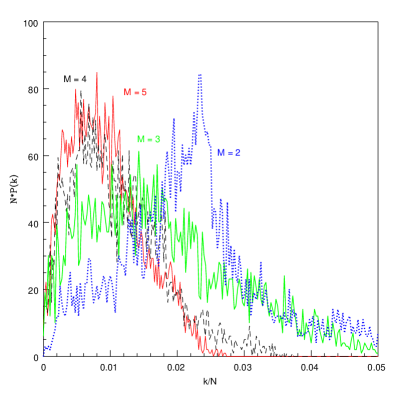
Figure 13: (Color online) Degree distributions (without error bar) of the RN constructed from the time series of Chen hyperchaotic attractor for $M=2$ (thick blue dotted line), $M=3$ (thick green solid line), $M=4$ (black dashed line) and $M=5$ (thin red solid line). For each $M$, the corresponding value of $\epsilon_{c}$ given in Table 1 is used for constructing the RN with $N=5000$.

We next show that the present scheme is efficient not only for low dimensional chaotic attractors, but also for the analysis of high dimensional and hyperchaotic systems as well. In Fig. 13, we show the degree distributions of the RN constructed from the time series of Chen hyperchaotic flow chen for $M$ varying from $2$ to $5$, with corresponding values of $\epsilon_{c}$. We generate the hyperchaotic time series with $5000$ data points using the standard set of parameters: $a=35$, $b=4.9$, $c=25$, $d=5$, $e=35$ and $k=100$. Note that the degree distributions for $M=4$ and $5$ are almost identical while that for lower $M$ values deviate, since the attractor dimension is $>3$. This is also a direct confirmation of our argument above that for a real world data whose dimension is unknown, one has to check for saturation of network measures by increasing the $M$ value. This is somewhat equivalent to finding the saturated $D_{2}$ value by increasing $M$ in the conventional nonlinear time series analysis.

Another important outcome of our scheme is that we are able to compare the characteristic measures derived from the RN of different chaotic attractors since the analysis is done using identical threshold for a fixed $M$. For example, the degree distribution of the RN typically characterises the structure of the attractor, as discussed above. Hence, a visual inspection of the degree distribution can provide some qualitative information on the structural complexities of standard low dimensional chaotic attractors, as shown in Fig. 14 and Fig. 15. The degree distribution in each case is the average from four RNs generated using different initial conditions for the attractor. From a comparison of the degree distributions in Fig. 14 one can infer that the Lorenz attractor is structurally more complex compared to the other three since the fluctuation in the probability density is maximum for it. More accurate results can be obtained from a quantitative analysis of the network measures.

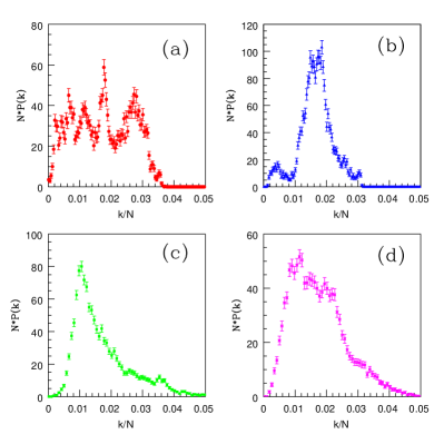
Figure 14: (Color online) Characteristic degree distributions of four standard low dimensional chaotic attractors for $M=3$. The systems are (a) Lorenz (b) Rössler (c) Duffing and (d) Ueda attractor. Standard parameter values given in spr are used for the generation of time series from Duffing and Ueda attractors. The average degree distribution for RNs generated from four initial conditions is shown in all cases.

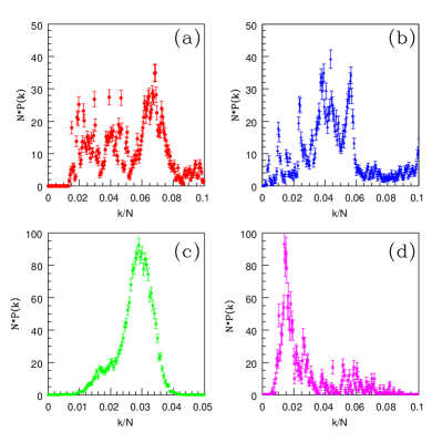
Figure 15: (Color online) Same as the previous figure for four standard chaotic maps, namely, (a) Henon (b) Lozi (c) Cat Map and (d) Logistic Map. For the logistic map in the fully chaotic regime, we use $M=1$ and $\epsilon_{c}=0.01$ which results in the high peak corresponding to that $\epsilon$ value. For all other cases, we use $M=2$.

For the logistic map, we use the fully chaotic region with $M=1$ and $\epsilon_{c}=0.01$ and hence the very large peak in the degree distribution corresponding to that $\epsilon$ value is due to Poisson statistics. The logistic map requires a special mention. For an attractor in one dimension, the Poisson value of $k/N\equiv\epsilon_{c}$, the threshold itself. In other words, for a random distribution in the unit interval, the degree distribution is typically a Poissonian around degree $k/N\equiv\epsilon_{c}$ in our scheme. However, for the RN from the logistic attractor, depending on the probability density variations, the number of degrees of any node can be $>>\epsilon_{c}$ or $<<\epsilon_{c}$. For example, from the figure, there are nodes with degree as high as $0.09$ and as low as $0.002$. The structure of the logistic attractor is actually characterized by ${{k}\over{N}}$ values $>\epsilon_{c}$.

V APPLICATIONS

So far, we have been discussing the construction and analysis of RN from chaotic time series. It is also important to know how effectively our scheme can be applied to time series data from the real world. An important difference is that for standard chaotic systems, the dimensionality of the system is known a priori and $M$ can be fixed accordingly while for real world data, this information is absent. In the conventional nonlinear time series analysis, one computes dynamical invariants as a function of $M$ and check for saturation with respect to $M$. For RN analysis, what is normally done is to use a sufficiently large value of $M$ to ensure a proper embedding of the underlying attractor gao1 . Our scheme indicates that a large $M$ requires a correspondingly large $N$ and $\epsilon_{c}$. However, the number of data points in real world time series is normally less (say, $<10000$) and contaminated by different types of noise. One of the advantages of RN analysis is that it is possible to get information regarding the underlying system from a time series with limited number of data points. Hence for practical implementation of the scheme for real world data, we suggest that it is better to start the computation taking a small $M$, go for higher dimensions successively and check for saturation of the network measures for two successive dimensions, rather than using a very high embedding dimension to start with.

To illustrate the potential applications of our approach, we consider two examples. In the first example, we show that the proposed scheme is capable of identifying the dimensionality of the underlying system and the presence of white noise in real world data. For this, we present the RN analysis of the light curves from a black hole system GRS 1915+105. The light curves from this black hole system have been classified into $12$ spectroscopic states by Belloni et al. bell and we take light curves from two representative states $\theta$ and $\chi$, which are shown in Fig. 16. In an earlier paper kph2 , we have shown by computing $D_{2}$ that the state $\theta$ has signatures of deterministic nonlinear behavior (with $D_{2}<3$) and $\chi$ is white noise. We construct the RN from the two time series for different values of $M$ starting from $M=2$ using the $\epsilon_{c}$ corresponding to each $M$ and compute the network measures in each case. We find that if the system is of finite dimension, the measures saturate beyond a certain $M$ which is taken as the dimension of the system. In Fig. 17, we show the rescaled degree distributions of the two light curves for $M=2,3$ and $4$. Note that the degree distributions for the two states are completely different. For the $\chi$ state, they are Poissonian and shows the typical shift without any saturation as $M$ increases, indicating pure white noise. On the other hand, the state $\theta$ is qualitatively different with the degree distributions getting saturated for $M=3$ and $4$ and remains stationary for any higher embedding dimension.

Due to the inherent non-subjectivity in the choice of $\epsilon_{c}$, the scheme is also ideal for the surrogate analysis using network measures CC and CPL as discriminating statistic to detect deterministic nonlinearity in real world data. It can be used as complementary to conventional analysis with measures like $D_{2}$ and $K_{2}$ and has the added advantage that the length of the data required is much less compared to conventional methods.

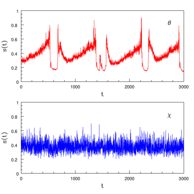
Figure 16: (Color online) Part of the astrophysical light curves from the black hole system GRS 1915 + 105 for two temporal states, $\theta$ and $\chi$ (Ref: xte.mit.edu/ ehm/1915_lightcurves.html).

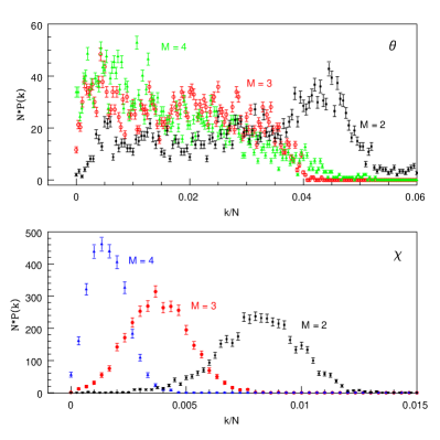
Figure 17: (Color online) Rescaled degree distributions computed from the RNs for the two light curves $\theta$ and $\chi$ for three $M$ values. The distributions are for $M=2$ (filled black squares), $M=3$ (open red circles) and $M=4$ (filled green triangles appearing in light gray shade in print) for $\theta$ state. The distributions for the three $M$ values for the $\chi$ state can be clearly distinguished, as indicated. In both cases, $N=3000$. Note that for the $\theta$ state the two degree distributions for $M=3$ and $4$ almost coincide.

As the second application, we consider detection of a dynamical transition using the RN measures derived from our method. This is known to be an important application of RNs dong1 ; kurt . The example we choose is the chaos-hyperchaos transition in a time delayed system, namely, the Mackey-Glass (M-G) system mack given by the equation:

$${{dx}\over{dt}}={{\beta x_{\tau_{D}}}\over{1+x_{\tau_{D}}^{n}}}-\gamma x$$ (18)

The constants $\beta,\gamma,\tau_{D}$ and $n$ are real numbers and $x_{\tau_{D}}$ represents the value of the variable $x$ at time $t-\tau_{D}$. Depending on the values of the parameters, the system displays a range of periodic, chaotic and hyperchaotic dynamics. We fix the parameters $\beta=2,\gamma=1,n=10$ with $\tau_{D}$ as the control parameter. As the value of the parameter $\tau_{D}$ increases, the asymptotic state of the system changes from periodic to chaotic and then to hyperchaos. We have recently shown kph5 using a dimensional analysis that the transition to hyperchaos occurs at a critical value $\tau_{D}=4.038$. Here we check whether the RN measures obtained from our scheme can detect this transition.

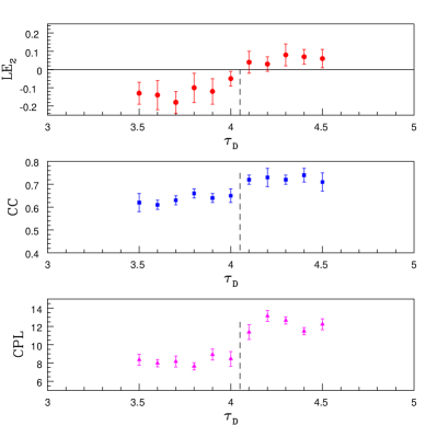
Figure 18: (Color online) Variation of the CPL and CC of the RN constructed by our scheme from the time series of M-G system for the range of $\tau_{D}$ values representing the transition from chaos to hyperchaos. Corresponding values of the second largest LE (denoted $LE_{2}$) are shown in the top panel. The dashed vertical line indicates the transition point.

To do the analysis, we first generate time series of length $100000$ from the system for $\tau_{D}$ values ranging from $3.5$ to $4.5$ increasing in steps of $0.1$. Each of this time series is then split up into $10$ time series of length $N_{T}=10000$. We construct RN from all these and compute the measures CC and CPL taking $M=4$ and $\epsilon=0.14$, which is the minimum $M$ value required for a hyperchaotic attractor (any higher embedding dimension is equally good). Using the TISEAN package hegg , we also compute the second largest Lyapunov Exponent (LE) (denoted $LE_{2}$) which crosses zero as the system cross over to hyperchaotic phase. The results of computations are shown in Fig. 18, where the vertical dashed line indicates the transition point. The error bar comes from the standard deviation of the values obtained from the ten time series used for each $\tau_{D}$. It is clear that the present scheme can detect the transition as both CC and CPL show a discontinuity at the transition point.

VI DISCUSSION AND CONCLUSION

Recurrence networks have become important statistical tools for characterising the structural properties of chaotic attractors. They are complex networks constructed from chaotic time series using a suitable scheme that maps information inherent in the time series into the network domain. One can then use the network based measures to quantify the geometric properties of the underlying attractor. The distinct advantages of such an exercise are that the network measures can be efficiently computed from less number of data points in the time series and these measures can also be used as complimentary to conventional measures of nonlinear time series analysis. Here we present a general scheme to construct the RN from a chaotic time series that can be applied equally well to time series from standard chaotic attractors as well as real world data. We use identical value of threshold to construct the RN from different time series for a given embedding dimension. The scheme is thus found to be suitable to compare the structural properties of two chaotic attractors by computing the statistical measures of the corresponding recurrence networks. To illustrate how the scheme can be implemented in practice, it is used for the analysis of light curves from a black hole system and to identify the transitions between two dynamical regimes in a time delayed system.

It is important to know the merits, limitations and potential applications of the proposed scheme for its proper implementation. Several methods have already been proposed in the literature for the construction of RN, as discussed in §I. These methods mainly differ in the criteria for the selection of $\epsilon_{c}$. The main aspects in our approach compared to the earlier methods are the uniform deviate transformation of the time series and the criterion used for the selection of $\epsilon_{c}$ with its linkage to embedding dimension $M$. These changes make it possible to look for a uniform critical threshold for different chaotic time series.

We do not claim that the RN constructed by our approach is optimum for all the different types of time series and applications. The critical range $\Delta\epsilon$ presented in Table 1 for each $M$ is an empirical choice resulting from the analysis on a limited number of nodes $(N<10000)$. It is primarily motivated to get a uniform range for different chaotic attractors as explained in §III and is not a rigorous result. Though we expect the range to be valid in general, it may require improvement for specific time series and more accurate applications. However, by getting an identical value of $\epsilon_{c}$ for different time series, we are able to achieve a certain level of non subjectiveness in the construction of RN, especially for the analysis of time series from the real world, as we have shown explicitly.

Another important outcome of the present approach not reported previously, is the realisation that the value of $\epsilon_{c}$ should be linked to $M$. This implies that the choice of $M$ is equally important for RN construction from time series and a very large value of $M$, as is generally believed, may not provide optimum result with limited number of data points. It is also interesting to note that there is always a part in the degree distribution of the RN from a chaotic attractor that corresponds to Poisson distribution where the $k$ values occur more by chance than by choice. Its position in the degree distribution depends on the choice of $\epsilon_{c}$ and $M$.

There are at least four important potential applications for our approach, three of which we have shown here explicitly:

i) to compare the structural properties of two chaotic attractors using network measures through the construction of RN

ii) to study the transition between two dynamical regimes as a control parameter is varied

iii) to identify the dimension of the underlying attractor from the analysis of time series data and

iv) for surrogate analysis using any of the RN measures as discriminating statistic where a non subjective comparison of the network measures from data and surrogates is required.

Finally, an important step forward in our analysis is to try and develop a similar scheme for RNs where the connections have weight factors. Here we have considered unweighted RNs so that the resulting adjacency matrix is binary. We hope that a weighted RN can unravel more information regarding the topological and structural properties of chaotic attractors. Another possible application of the scheme, that is important in the analysis of real world data, is to study the effect of noise on RN and the measures derived from it. These works are currently in progress and will be reported elsewhere.

- (1) P. Erdős and A. Rényi, On the evolution of random graphs, Publ.Math.Inst.Hung.Acad. Sci. 5, 17-61(1960)
- (2) M. E. J. Newman, Networks: An Introduction, (Oxford Univ. Press, New York, 2010)
- (3) D. J. Watts, Six Degrees: The Science of a Connected Age, (Norton, New York, 2003)
- (4) R. Albert and A. L. Barabasi, Statistical Mechanics of Complex Networks, Rev. Mod. Phys. 74, 47-97(2002)
- (5) S. Boccaletti, V. Latora, Y. Moreno, M. Chavez and D. U. Hwang, Complex Networks: Structure and Dynamics, Phys. Reports 424, 175-308(2006)
- (6) S. H. Strogatz, Exploring complex networks, Nature 410, 268-276(2001)
- (7) B. Barzel and A. L. Barabasi, Universality in network dynamics, Nature Phys. 9, 673-681(2013)
- (8) J. Zhang and M. Small, Complex networks from pseudoperiodic time series: topology versus dynamics, Phys. Rev. Lett. 96, 238701(2006)
- (9) L. Lacasa, B. Luque, F. Ballesteris, J. Luque and J. C. Nuno, From time series to complex networks: the visibility graph, Proc. Natl. Acad. Sci. USA 105, 4972-4975(2008)
- (10) G. Nicolis, G. Cantu and C. Nicolis, Dynamical aspects of interaction networks, Int. J. Bif. Chaos 15, 3467-3480(2005)
- (11) N. Marwan, J. F. Donges, Y. Zou, R. V. Donner and J. Kurths, Complex network approach for recurrence analysis of time series, Phys. Lett. A 373, 4246-4254(2009)
- (12) Y. Yang and H. Yang, Complex network based time series analysis, Physica A 387, 1381-1386(2008)
- (13) X. Xu, J. Zhang and M. Small, Super family phenomena and motifs of networks induced from time series, Proc. Natl. Acad. Sci. USA 105, 19601-5(2008)
- (14) R. V. Donner, J. Heitzig, J. F. Donges, Y. Zou, N. Marwan and J. Kurths, The geometry of chaotic dynamics-A complex network perspective, European Phys. J. B 84, 653-672(2011)
- (15) R. V. Donner, Y. Zou, J. F. Donges, N. Marwan and J. Kurths, Recurrence networks: A novel paradigm for nonlinear time series analysis, New J. Phys. 12, 033025(2010)
- (16) R. V. Donner, M. Small, J. F. Donges, N. Marwan, Y. Zou, R. Xiang and J. Kurths, Recurrence based time series analysis by means of complex network methods, Int. J. Bif. Chaos 21, 1019-46(2011)
- (17) Y. Zou, R. V. Donner, J. F. Donges, N. Marwan and J. Kurths, Identifying complex periodic windows in continuous time dynamical systems using recurrence based methods, CHAOS 20, 043130(2010)
- (18) J. F. Donges, R. V. Donner, K. Rehfeld, N. Marwan, M. H. Trauth and J. Kurths, Identification of dynamical transitions in marine palaeoclimate records by recurrence network analysis, Nonlinear Proc. Geophys. 18, 545-562(2011)
- (19) Z. Gao and N. Jin, Flow pattern identification and nonlinear dynamics of gas liquid two phase flow in complex networks, Phys. Rev. E 79, 066303(2009)
- (20) N. Marwan, N. Wessel, U. Meyerfeldt, A. Schirdewan and J. Kurths, Recurrence plot measures of complexity and its application to heart rate variability data, Phys. Rev. E 66, 026702(2002)
- (21) R. Avila, A. Gapelyuk, N. Marwan, T. Walther, H. Stepan, J. Kurths and N. Wessel, Classification of cardio-vascular time series based on different coupling structures using recurrence network analysis, Philos. T. Roy. Soc. A 371, 20110623(2013)
- (22) N. Marwan, M. H. Trauth, M. Vuille and J. Kurths, Comparing modern and Pleistocene ENSO-like influences in NW Argentina using nonlinear time series analysis, Clim. Dynam. 21, 317-326(2003)
- (23) W. V. Zolotova, D. I. Ponyavin, N. Marwan and J. Kurths, Long term asymmetry in the wings of the butterfly diagram, Astron. and Astrophys. 505, 197-201(2009)
- (24) J. P. Eckmann, S. O. Kamphorst and D. Ruelle, Recurrence plot of dynamical systems, Europhys Letters 5, 973-977(1987)
- (25) P. Grassberger and I. Procaccia, Measuring the strangeness of strange attractors, Physica D 9, 189-208(1983)
- (26) N. Marwan, M. C. Romano, M. Thiel and J. Kurths, Recurrence plot for the analysis of complex systems, Phys. Reports 438, 237-329(2007)
- (27) A. Giuliani, R. Benigni, J. Zbilut, C. Webber, P. Sirabella and A. Colosimo, Nonlinear signal analysis methods in the elucidation of protein sequence structure relationships, Chemical Rev. 102, 1471-1492(2002)
- (28) A. Facchini, C. Mocenni, N. Marwan, A. Vicino and E. Tiezzi, Nonlinear time series analysis of dissolved oxygen in the Orbetello Lagoon, Ecological Modelling 203, 339-348(2007)
- (29) G. Litak, J. T. Sawicki and R. Kasperek, Cracked rotor detection by recurrence plots, Nondestructive Testing and Eval. 24, 347-351(2009)
- (30) M. Thiel, M. C. Romano, P. L. Read and J. Kurths, Estimation of dynamical invariants without embedding by recurrence plots, CHAOS 14, 234-243(2004)
- (31) R. V. Donner, Y. Zou, J. F. Donges, N. Marwan and J. Kurths, Ambiguities in recurrence based complex network representations of time series, Phys. Rev. E 81, 015101(R)(2010)
- (32) Z. Gao and N. Jin, Complex network from time series based on phase space reconstruction, CHAOS 19, 033137(2009)
- (33) S. Schinkel, O. Dimigen and N. Marwan, Selection of recurrence threshold for signal detection, European Phys. J. ST 164, 45-53(2008)
- (34) J. F. Donges, J. Heitzig, R. V. Donner and J. Kurths, Analytical framework for recurrence network analysis of time series, Phys. Rev. E 85, 046105(2012)
- (35) D. Eroglu, N. Marwan, S. Prasad and J. Kurths, Finding recurrence networks threshold adaptively for a specific time series, Nonlin. Processes Geophys. 21, 1085-1092(2014)
- (36) K. P. Harikrishnan, R. Misra, G. Ambika and A. K. Kembhavi, A non-subjective approach to the GP algorithm for analysing noisy time series, Physica D 215, 137-145(2006)
- (37) K. P. Harikrishnan, R. Misra and G. Ambika, Nonlinear time series analysis of the light curves from the black hole system GRS 1915+105, Research in Astr. and Astrophys. 11, 71-90(2011)
- (38) K. P. Harikrishnan, R. Misra and G. Ambika, Revisiting the box counting algorithm for the correlation dimension analysis of hyperchaotic time series, Comm. Nonlinear Sci. Num. Simulations 17, 263-276(2012)
- (39) K. P. Harikrishnan, R. Misra and G. Ambika, Combined use of correlation dimension and entropy as discriminating measures for time series analysis, Comm. Nonlinear Sci. Num. Simulations 14, 3608-3614(2009)
- (40) J. C. Sprott, Chaos and Time Series Analysis (Oxford Univ. Press, Oxford, 2003)
- (41) T. Belloni, M. Klein-Wolt, M. Mendez, M. van der Klis and J. van Paradjis, A model-independent analysis of the variability of GRS 1915+105, Astronomy and Astrophys. 355, 271-290(2000)
- (42) Y. Zou, J. Heitzig, R. V. Donner, J. F. Donges, J. D. Farmer, R. Meucci, S. Euzzor, N. Marwan and J. Kurths, Power laws in recurrence networks in dynamical systems, Europhys. Letters 98, 48001-6(2012)
- (43) Z. Chen, Y. Yang, G. Qi and Z. Yuan, A novel hyperchaos system only with one equilibrium, Phys. Lett. A 360, 696-701(2007)
- (44) N. Marwan and J. Kurths, Complex network based techniques to identify extreme events and (sudden) transitions in spatio-temporal systems, CHAOS 25, 097609(2015)
- (45) M. C. Mackey and L. Glass, Oscillation and chaos in physiological controll systems, Science 197, 287-289(1977)
- (46) K. P. Harikrishnan, R. Misra and G. Ambika, On the transition to hyperchaos and the structure of hyperchaotic attractors, European Phys. J. B 86, 394(2013)
- (47) R. Hegger, H. Kantz and T. Schreiber, Practical implementation of nonlinear time series methods: The TISEAN package, CHAOS 9, 413(1999)