Anisotropic radiation from accretion disc-coronae in active galactic nuclei

Abstract

In the unification scheme of active galactic nuclei (AGN), Seyfert 1s and Seyfert 2s are intrinsically same, but they are viewed at different angles. However, the Fe K$\alpha$ emission line luminosity of Seyfert 1s was found in average to be about twice of that of Seyfert 2s at given X-ray continuum luminosity in the previous work (Ricci et al., 2014). We construct an accretion disc-corona model, in which a fraction of energy dissipated in the disc is extracted to heat the corona above the disc. The radiation transfer equation containing Compton scattering processes is an integro-differential equation, which is solved numerically for the corona with a parallel plane geometry. We find that the specific intensity of X-ray radiation from the corona changes little with the viewing angle $\theta$ when $\theta$ is small (nearly face-on), and it is sensitive to $\theta$ if the viewing angle is large ($\theta\ga 40^{\circ}$). The radiation from the cold disc, mostly in infrared/optical/UV bands, is almost proportional to $\cos\theta$ when $\theta$ $\la 40^{\circ}$, while it decreases more rapidly than $\cos\theta$ when $\theta\ga 40^{\circ}$ because of strong absorption in the corona in this case. For seyfert galaxies, the Fe K$\alpha$ line may probably be emitted from the disc irradiated by the X-ray continuum emission. The observed equivalent width (EW) difference between Seyfert 1s and Seyfert 2s can be reproduced by our model calculations, provided Seyfert 1s are observed in nearly face-on direction and the average inclination angle of Seyfert 2s $\sim 65^{\circ}$.

1 Introduction

According to the unification scheme of active galactic nuclei (AGN), Seyfert 1s (Sy1s) and 2s (Sy2s) are intrinsically same but viewed at different angles, which leads to different observational features (Antonucci, 1993). Liu & Wang (2010) found that the Fe K$\alpha$ line luminosities of Compton-thin Seyfert 2 galaxies are in average 2.9 times weaker than their Seyfert 1 counterparts. Ricci et al. (2014) found that the Fe K$\alpha$ line luminosities of Sy1s are about twice of those for Sy2s at a given X-ray continuum luminosity ($10-50$ keV). The reason is still unclear. One possibility is that such difference is caused by anisotropic X-ray emission from these sources. Indeed, the orientation dependence of emission from AGN has been found and studied for a long time. Nemmen & Brotherton (2010) explored the uncertainty of the bolometric corrections of quasars with different viewing angles based on the accretion disc models of Hubeny et al. (2000), and found that a value of the bolometric luminosity for a quasar viewing at an angle of $\approx 30^{\circ}$ will result in $\approx 30\%$ systematic error, if the emission from the quasar is assumed to be isotropic. Runnoe, Shang, & Brotherton (2013) analyzed a sample of radio-loud quasars and found that the quasar luminosity changes with orientation. The sources viewed in the face-on direction are brighter than the edge-on sources by a factor of 2-3. Zhang (2005) explained the observed anticorrelation between type ${\rm II}$ fraction and the X-ray luminosity in 2$-$10 keV based on the AGN unification model with only one intrinsic luminosity function for these two types of AGNs. Recently, DiPompeo et al. (2014) used two observed luminosity functions to investigate the intrinsic quasar luminosity function with the correction of a simple projection effect for the anisotropic emission of accretion disc. They concluded that the orientation dependence is the most important one among several potential corrections. They also claimed that more complex model of anisotropy may strengthen the orientation effect.

The black hole accretion disc-corona model has been widely used to explain both the thermal optical/UV and the power-law hard X-ray emission in the spectral energy distributions (SEDs) of active galactic nuclei (AGNs) (Galeev, Rosner, & Vaiana, 1979; Haardt & Maraschi, 1991, 1993; Nakamura & Osaki, 1993; Svensson & Zdziarski, 1994; Liu, Mineshige, & Shibata, 2002; Liu, Mineshige, & Ohsuga, 2003; Cao, 2009; You, Cao, & Yuan, 2012) and galactic black hole candidates (GBHC) (Esin et al., 1998; Dove, Wilms, & Begelman, 1997; Dove et al., 1997; Nayakshin & Dove, 2001). Although there are different physical mechanisms proposed in the previous works for heating the corona and the interactions between the cold disc and the hot corona, the disc-corona is mostly structured as a sandwich-like cylindrically symmetric system (Begelman & McKee, 1990; Balbus & Hawley, 1991; Meyer & Meyer-Hofmeister, 1994; Zycki, Collin-Souffrin, & Czerny, 1995; Witt, Czerny, & Zycki, 1997; Di Matteo, 1998; Di Matteo, Celotti, & Fabian, 1999; Dullemond, 1999; Różańska & Czerny, 2000; Merloni & Fabian, 2001, 2002). The optically thin and geometrically thick hot coronae are vertically connected to the both sides of an optically thick and geometrically thin accretion disc. It was also suggested that such hot coronae may play an important role in launching relativistic jets observed in X-ray binaries/AGN (e.g., Merloni & Fabian, 2002; Cao, 2004; Zdziarski et al., 2011; Wu et al., 2013; Cao, 2014). In the accretion disc-corona system, the observed thermal optical/UV emission is believed to originate from the blackbody radiation of the thin disc passing through the hot corona. A small fraction of soft photons are inverse Compton scattered by the hot electrons in the corona, which contribute to the observed power-law hard X-ray emission of the system. Moreover, the temperature of the electron in the transition layer between the corona and the disc experiences a rapid decrease from $\sim 10^{8-9}$K (the hot corona) to $\sim 10^{4-5}$K (the cold disc), the thermal X-ray line emission may be produced in such transition zone (Xu, 2013). In most previous works, either the cooling rate in the corona or the spectra from the accretion flow are calculated assuming the corona to be one parallel-plane. The inverse Compton scattering is often computed by the Monte Carlo simulation based on the escape probability method (Pozdniakov, Sobol, & Siuniaev, 1977; Kawanaka, Kato, & Mineshige, 2008; Liu, Mineshige, & Ohsuga, 2003; Cao, 2009).

Assuming that a fraction of viscously dissipated energy in the disc is transported into the corona (probably by magnetic fields), we can calculate the structure of the disc-corona accretion with a set of equations of the accretion flow, such as, energy equation, angular momentum equation, continuity equation, and state equation, etc., if the model parameters are given. Then, the emitted spectra from the accretion flow can be calculated. In this work, we explore the angle-dependent emission of the accretion disc-corona system in more detail, by solving a set of equations describing disc-corona structure and the equation of radiation transfer in the corona simultaneously. The change of the spectra with the viewing angle is explored in detail. Our results are compared with the X-ray observations of Sy1s and Sy2s. The disc-corona model employed in this work is briefly described in §2. The calculation method is introduced in §3. We show the results and discussion in §4 and 5.

2 The disc-corona accretion model

The accretion disc-corona model used in this work is described in the previous works (Cao, 2009; Xu, 2013). The detailed model description and calculating approach can be found in Cao (2009). Here we only briefly summarize the main features of the model. The energy equation of the cold thin disc is

$$Q_{\rm dissi}^{+}-Q_{\rm cor}^{+}+\frac{1}{2}(1-a_{\rm r})Q_{\rm cor}^{+}=\frac{4\sigma T^{4}_{\rm disc}}{3\tau},$$ (1)

where,

$$Q_{\rm dissi}^{+}=\frac{3}{8\pi}\dot{M}\Omega_{\rm k}^{2}(R)\left[1-\left(\frac{R_{\rm in}}{R}\right)^{1/2}\right],$$ (2)

is the gravitational power dissipated in unit surface area of the accretion disc at radius $R$ [where, $\Omega_{\rm k}(R)$ is the Keplerian velocity, $R_{\rm in}=3R_{\rm S}$, $R_{\rm S}=2GM_{\rm bh}/c^{2}$ is the Schwarzschild radius for a black hole of mass $M_{\rm bh}$, and $\dot{M}$ is the mass accretion rate of the black hole]. The third term in the left side of equation (1) represents that about half of the power dissipated in the corona is radiated back into the disc by Compton scattering, and the reflection albedo of the disc $a_{\rm r}=0.15$ is adopted in the calculations. The right side of the equation represents the power radiated from the cold disc via blackbody radiation, where $T_{\rm disc}$ is the effective temperature in the mid-plane of the disc, and $\tau$ is the optical depth in vertical direction of the disc. The continuity equation of the disc is

$$-4\pi RH_{\rm d}(R)\rho(R)v_{\rm R}(R)=\dot{M},$$ (3)

where $H_{\rm d}(R)$ is the half thickness of the disc, $\rho(R)$ is the mean density of the disc, and $v_{\rm R}(R)$ is the radial velocity of the accretion flow at radius $R$. The state equation of the gas in the disc is

$$p_{\rm tot}=p_{\rm gas}+p_{\rm rad}=\frac{\rho kT_{\rm disc}}{\mu m_{\rm p}}+\frac{1}{3}aT^{4}_{\rm disc},$$ (4)

where $\mu=(1/\mu_{\rm i}+1/\mu_{\rm e})^{-1}$, $\mu_{\rm i}=1.23$ and $\mu_{\rm e}=1.14$ are adopted. The half thickness of the disc $H_{\rm d}$ is

$$H_{\rm d}=c_{\rm s}/\Omega_{\rm k}=\frac{\sqrt{p_{\rm tot}/\rho}}{\Omega_{\rm k}}.$$ (5)

The energy equation of the corona is

$$Q^{+}_{\rm cor}=Q^{\rm ie}_{\rm cor}+\delta Q^{+}_{\rm cor}=F^{-}_{\rm cor},$$ (6)

where $Q^{\rm ie}_{\rm cor}$ is the energy transfer rate from the ions to the electrons via Coulomb collisions (see equation 11 in Cao, 2009) , $\delta$ is the fraction of the energy directly heats the electron, $F_{\rm cor}^{-}=F^{-}_{\rm syn}+F^{-}_{\rm brem}+F^{-}_{\rm Comp}$ is the cooling rate in unit surface area of the corona via synchrotron, bremsstrahlung, and Compton emissions. The value of $\delta$ can be as high as $\sim 0.5$ by magnetic reconnection, if the magnetic field in the plasma is strong (Bisnovatyi-Kogan & Lovelace, 1997, 2000). Almost all the power dissipated in the hot corona is radiated away locally, which means that the radiated power in the corona is independent of the value $\delta$, and the temperature and density of the electrons in the corona are almost insensitive with this parameter (see Cao, 2009, for the discussion). In the accretion disc-corona model, the detailed physical mechanism for generating the energy source and heating the corona is still unclear, though there are some assumptions of corona heating processes, such as, magnetic fields reconnection assumed in the previous works (e.g. Di Matteo, 1998; Di Matteo, Celotti, & Fabian, 1999; Merloni & Fabian, 2001, 2002; Cao, 2009; Xu, 2013). To avoid the complexity, we introduce a parameter, $f_{\rm cor}$, the ratio of the power dissipated in the corona, $Q_{\rm cor}^{+}$, to the gravitational power dissipated in the disc, $Q_{\rm dissi}^{+}$,

$$Q_{\rm cor}^{+}=f_{\rm cor}Q_{\rm dissi}^{+},$$ (7)

in our model calculations.

3 Radiative transfer in the corona

We consider a parallel plane geometry of the corona above/below the disc. The cooling processes in the corona include Compton, bremsstrahlung, and synchrotron emissions. The incident photons from the disc at $z=H_{\rm d}$ are assumed to be blackbody radiation. For simplicity, the electron density and temperature of the corona are assumed to be constant in the $z$ direction.

3.1 Radiative transfer equation

The radiative transfer equation of the corona is,

$$\frac{dI_{\nu}(z,\mu)}{ds}=-I_{\nu}(z,\mu)(\kappa_{\nu}^{\rm ff}+\kappa_{\rm T})+j_{\nu}^{\rm ff}+j_{\nu}^{\rm C},$$ (8)

where $ds=dz/\mu$, $\mu=\cos\theta$, $\theta$ is the angle of the photon with respect to the vertical direction of the disc, and $I_{\nu}(z,\mu)$ is the specific intensity. For the different absorption and emission processes included in the corona, we have the combined absorption and emission coefficients, $\kappa_{\nu}=\kappa_{\nu}^{\rm ff}+\kappa_{\rm T}$, is the total absorption coefficient including free-free(bremsstrahlung+synchrotron) absorption and Thomson scattering, $j_{\nu}=j_{\nu}^{\rm ff}+j_{\nu}^{\rm C}$, is the emission coefficient (emissivity) including free-free(bremsstrahlung+synchrotron) emission and Comptonization emission. We can calculate $I_{\nu}(z,\mu)$ when the structure of the corona, such as electron temperature $T_{\rm e,cor}(r)$ and electron density $n_{\rm e,cor}(r)$, are given.

3.2 Absorption and emission coefficients

The absorption coefficient of Thomson scattering is $\kappa_{\rm T}=n_{\rm e,cor}\sigma_{\rm T}$, where $\sigma_{\rm T}$ is Thomson cross section. The absorption coefficient including bremsstrahlung and synchrotron processes can be described as

$$\kappa_{\nu}^{\rm ff}=j_{\nu}^{\rm ff}/B_{\nu},$$ (9)

where $B_{\nu}$ is the blackbody emissivity,

$$B_{\nu}(T)=\frac{2h\nu^{3}/c^{2}}{\exp{(h\nu/kT)-1}},$$ (10)

and $j_{\nu}^{\rm ff}=(\chi_{\nu}^{\rm Brem}+\chi_{\nu}^{\rm Syn})/4\pi$ is the emission coefficient of bremsstrahlung and synchrotron processes. The bremsstrahlung emissivity $\chi_{\nu}^{\rm Brem}$ and synchrotron emissivity $\chi_{\nu}^{\rm Syn}$ are taken from Narayan & Yi (1995) and Manmoto (2000).

The bremsstrahlung emissivity is given by

$$\chi_{\nu}^{\rm brem}=q_{\rm brem}^{-}\bar{\rm G}~{}{\exp}{\left(\frac{h\nu}{kT_{\rm e}}\right)},$$ (11)

where $\bar{\rm G}$ is the Gaunt factor as in Rybicki & Lightman (1986),

$$\bar{\rm G}=\frac{h}{kT_{\rm e}}\left(\frac{3}{\pi}\frac{kT_{\rm e}}{h\nu}\right)^{1/2}~{}~{}~{}~{}~{}~{}{\rm for}~{}~{}\frac{kT_{\rm e}}{h\nu}<1,$$ (12)

$$\bar{\rm G}=\frac{h}{kT_{\rm e}}\frac{\sqrt{3}}{\pi}\ln\left(\frac{4}{\zeta}\frac{kT_{\rm e}}{h\nu}\right)~{}~{}~{}~{}~{}~{}{\rm for}~{}~{}\frac{kT_{\rm e}}{h\nu}>1.$$ (13)

The bremsstrahlung cooling rate per unit volume $q_{\rm brem}^{-}$ consists of electron-ion and electron-electron rates,

$$q_{\rm brem}^{-}=q_{\rm ei}^{-}+q_{\rm ee}^{-}.$$ (14)

The electron-ion cooling rate is

$$q_{\rm ei}^{-}=1.25n_{\rm e}^{2}\sigma_{\rm T}c\alpha_{\rm f}m_{\rm e}c^{2}F_{\rm ei}(\theta_{\rm e}),$$ (15)

where $\alpha_{\rm f}$ is the fine-structure constant, $\theta_{\rm e}=kT_{\rm e}/m_{\rm e}c^{2}$ is the dimensionless electron temperature, and the function $F_{\rm ei}$ has the form

$$F_{\rm ei}(\theta_{\rm e})=4\left(\frac{2\theta_{\rm e}}{\pi^{3}}\right)^{1/2}(1+1.781\theta_{\rm e}^{1.34})~{}~{}~{}~{}~{}~{}{\rm for}~{}~{}\theta_{\rm e}<1,$$ (16)

$$F_{\rm ei}(\theta_{\rm e})=\frac{9\theta_{\rm e}}{2\pi}[\ln(1.123\theta_{\rm e}+0.48)+1.5]~{}~{}~{}~{}~{}~{}{\rm for}~{}~{}\theta_{\rm e}>1.$$ (17)

The electron-electron cooling rate is

$$q_{\rm ee}^{-}=n_{\rm e}^{2}cr_{\rm e}^{2}\alpha_{\rm f}c^{2}\frac{20}{9\pi^{1/2}}(44-3\pi^{2})\theta_{\rm e}^{3/2}\\ (1+1.1\theta_{\rm e}+\theta_{\rm e}^{2}-1.25\theta_{\rm e}^{5/2})$$

$$~{}~{}{\rm for}~{}~{}\theta_{\rm e}<1,$$ (18)

$$q_{\rm ee}^{-}=n_{\rm e}^{2}cr_{\rm e}^{2}\alpha_{\rm f}c^{2}24\theta_{\rm e}(\ln 1.1232\theta_{\rm e}+1.28)~{}~{}{\rm for}~{}~{}\theta_{\rm e}>1,$$ (19)

where $r_{\rm e}=e^{2}/m_{\rm e}c^{2}$ is the classical electron radius.

The synchrotron emissivity is given by

$$\chi_{\nu}^{\rm syn}=4.43\times 10^{-30}\frac{4\pi n_{\rm e}\nu}{K_{2}(1/\theta_{\rm e})}I^{\prime}(\frac{4\pi m_{\rm e}c\nu}{3eB\theta_{\rm e}^{2}}),$$ (20)

and the function $I^{\prime}(x)$ is given by

$$I^{\prime}(x)=\frac{4.0505}{x^{1/6}}(1+\frac{0.4}{x^{1/4}}+\frac{0.5316}{x^{1/2}})\exp(-1.8899x^{1/3}),$$ (21)

where $K_{2}$ is the second order modified Bessel function, $B$ is the magnetic field strength. For the equipartition magnetic field case, we have $B=\sqrt{8\pi p_{\rm gas,cor}}$ ($p_{\rm gas,cor}$ is the gas pressure in the corona).

The emissivity of the inverse Compton scattering is calculated with the method proposed in Coppi & Blandford (1990),

$$j_{\nu}^{\rm C}=\frac{f_{\nu}(T_{\rm e},n_{\rm e},I_{\nu^{\prime}})}{4\pi},$$ (22)

where

$$I_{\nu^{\prime}}=\int_{-1}^{1}{I_{\nu^{\prime}}(z,\mu)\kappa_{\rm T}2\pi d\mu},$$ (23)

is the seed photon intensity of the unit volume including incident photons from all the directions.

3.3 Numerical solution to the radiative transfer equation

The radiative transfer equation (8) is an integro-differential equation. For a given disc-corona structure (including temperatures and densities of the electrons and ions, half thicknesses of the disc $H_{\rm d}$ and thicknesses of the corona $H_{\rm cor}$, etc.), one can solve this equation by iterations (e.g., Cao et al., 1998). An initial solution can be obtained by solving the equation neglecting the Compton scattering term, i.e.,

$$\frac{dI_{\nu}(z,\mu)}{ds}=-I_{\nu}(z,\mu)(\kappa_{\nu}^{\rm ff}+\kappa_{\rm T})+j_{\nu}^{\rm ff}.$$ (24)

We solve the above equation numerically for the corona with the boundary condition at the disc surface,

$$I_{\nu}(z=H_{\rm d},\mu)=B_{\nu}(T_{\rm d}^{\rm s}),$$ (25)

in the range $0<\mu<1$, where $T_{\rm d}^{\rm s}$ is the temperature of the disc surface, and the boundary condition at the upper surface of the corona,

$$I_{\nu}(z=H_{\rm d}+H_{\rm cor},\mu)=0,$$ (26)

in the range $-1<\mu<0$. With derived initial solution, we calculate the emissivity of the inverse Compton scattering from equations (22) and (23), and solve equation (8) numerically. With derived $I_{\nu}(z,\mu)$, the emissivity of the Compton emission can be re-calculated with equations (22) and (23). We find that the final solution can be achieved after several iterations when the solutions converge.

Integrating the intensities over the different directions ($\mu=\cos\theta$) and frequencies $\nu$, the energy loss via radiation from the upper and lower surfaces of the corona can be calculated by

$$Q_{\rm cor}^{\rm rad}=\int_{\nu}d\nu\int_{0}^{1}{I_{\nu}(z=H_{\rm d}+H_{\rm cor},\mu)2\pi\mu d\mu}$$

$$+\int_{\nu}d\nu\int_{-1}^{0}{I_{\nu}}(z=H_{\rm d},\mu)2\pi\mu d\mu.$$ (27)

Subtracting the incident blackbody radiation from the thin disc,

$$Q_{\rm disc}^{-}=\int_{\nu}\pi B_{\nu}d\nu,$$ (28)

we obtain the cooling rate in unit surface area of the corona,

$$F_{\rm cor}^{-}=Q_{\rm cor}^{\rm rad}-Q_{\rm disc}^{-}.$$ (29)

Given the black hole mass $M_{\rm bh}$, the dimensionless mass accretion rate $\dot{m}$ ($\dot{m}=\dot{M}/\dot{M}_{\rm Edd}$, where $\dot{M}_{\rm Edd}=L_{\rm Edd}/0.1c^{2}$), and the fraction of the energy directly heats the electron $\delta$, we can derive the disc structure (such as, the effective temperature in the mid-plane of the disc, the density in the disc, and the half thickness of the disc, etc.) as a function of radius $R$ from equations (1)-(5), and equation (7), when the ratio of the power dissipated in the corona $f_{\rm cor}$ is specified. The structure of the corona (such as, temperatures and densities of the electrons and ions, scaleheight of the corona) can be derived with equations (6) and (29) under the assumption of equipartition of the magnetic pressure and the gas pressure in the corona. We assume the temperature of the ions in the corona $T_{\rm i,cor}=0.9T_{\rm vir}=0.9GMm_{\rm p}/3kR$ in this work as that in Cao (2009). Thus, the accretion disc-corona structure is available by solving the radiation transfer equation together with disc-corona equations described in §2.

The specific intensity from the corona at a certain radius $R$ is obtained as a function of direction and frequency of the photons. Integrating the intensity over the whole surface of the corona, the specific luminosity emitted from the corona per steradian is

$$\frac{dL_{\nu}}{2\pi d\mu}=\int\mu I_{\nu}(z=H_{\rm d}+H_{\rm cor},\mu)2\pi rdr.$$ (30)

Thus, we can obtain the direction-dependent spectrum of an accretion disc-corona system for a set of given disc parameters.

4 Results

We adopt the model parameters as follows, the black hole mass $M_{\rm bh}=10^{8}M_{\odot}$, the maximum radius of the disc-corona flow $R_{\rm cormax}=100R_{\rm S}$, and the fraction of energy directly heated the electron $\delta=0.5$, are fixed in all cases. The mass accretion rate $\dot{m}$ and the ratio of the power dissipated in the corona $f_{\rm cor}$ are taken as two free parameters in our model calculations.

In Figure 1, we show the emergent spectra for four disc-corona accretion models with different values of parameters $\dot{m}$ and $f_{\rm cor}$. The values of the two parameters in the models are, model (a): $\dot{m}=0.1$ and $f_{\rm cor}=0.1$, model (b): $\dot{m}=0.1$ and $f_{\rm cor}=0.3$, model (c): $\dot{m}=0.5$ and $f_{\rm cor}=0.06$, and model (d): $\dot{m}=0.5$ and $f_{\rm cor}=0.1$. For each model, we plot the emergent spectra observed in five different directions with the lines in different types and colors. The spectra from $\theta=87^{\circ},84^{\circ},76^{\circ},50^{\circ}$, and $2^{\circ}$ are shown with black dashed, cyan dotted, magenta dash-dotted, green thin solid, and blue thin dash-dotted lines, respectively. The corresponding value of $\theta$ is denoted near each spectrum. The red thick solid line is the spectra integrated over the directions from $\mu=0$ to $\mu=1$. The four vertical dotted lines represent the four typical frequency points corresponding to $2500{\rm\AA}$, 0.1 keV, 2 keV, and 10 keV, respectively. We can see from these figures that the spectra from different emitting directions are different both in the luminosity and the spectral shape. The luminosity decreases with the increasing viewing angle between the emitting photons and the axis of the accretion disc, $\theta$. The spectral shapes are similar in almost all bands but very different between the optical/UV ($\sim 2500{\rm\AA}$) and soft X-ray band ($0.1\sim 1$ keV).

The different values of mass accretion rate $\dot{m}=0.1$ and $\dot{m}=0.5$ are adopted in Figure 1(a) and Figure 1(d), respectively, while the values of all other parameters are the same in these two figures. The larger the mass accretion rate adopted, the stronger and harder the spectra are. The different values of $f_{\rm cor}=0.1$ and $f_{\rm cor}=0.3$ are adopted in Figure 1(a) and Figure 1(b), respectively, while the values of all other parameters are the same in these two figures. We find that the change of the spectra with $f_{\rm cor}$ is also evident. The larger the value of $f_{\rm cor}$ adopted, the harder the spectra are.

The spectral shapes plotted in the four panels of Figure 1 show a certain degree of degeneracy of the two parameters $\dot{m}$ and $f_{\rm cor}$. Different combinations of these two parameters may give very similar spectral shapes, but these can be distinguished by the different luminosity, which is directly controlled by $\dot{m}$.

In order to study the change of spectra with the viewing direction, we calculate some typical quantities of the observed spectra, including the observed bolometric luminosity $L_{\rm bol}$, the spectral luminosity at optical/UV band ($\lambda$=2500 $\rm\AA$) $L_{\rm o}$, and the spectral luminosity at X-ray band ($E=2$ keV) $L_{\rm x}$. The optical/UV to X-ray power index $\alpha_{\rm ox}$ is defined as

$$\alpha_{\rm ox}=-\frac{\log L_{\nu(2500~{}{\rm\AA})}/L_{\nu(2~{}{\rm keV})}}{\log\nu(2500~{}{\rm\AA})/\nu(2~{}\rm{keV})},$$ (31)

and the X-ray spectral index between 2 keV and 10 keV, $\alpha_{\rm x}$ (defined as $L_{\nu,{\rm x}}^{(2-10~{}{\rm keV})}\propto{\nu}^{-\alpha_{\rm x}}$). The changes of these quantities with the viewing angles are plotted in Figures 2-5.

In Figure 2, we plot the change of observed bolometric luminosity with viewing angle. The red solid, green dashed, cyan dotted, and black dash-dotted lines correspond to the four models (a)-(d), respectively. The blue thin dashed line indicates a simple relation as $L_{{\rm bol}}\propto\cos\theta$ representing the area-projection effect.

In Figures 3 and 4, we plot the changes of observed spectral luminosities at optical/UV band ($\lambda=2500{\rm\AA}$) and X-ray (2 KeV) band with the viewing angle. The red solid, green dashed, cyan dotted, and black dash-dotted lines correspond to the four models (a)-(d), respectively. The blue thin dashed lines also represent simple relations as $L_{\rm o}\propto\cos\theta$ and $L_{\rm x}\propto\cos\theta$. We find that the two spectral luminosities (optical and X-ray bands) show different changes with the viewing angle $\theta$. The X-ray luminosity $L_{\rm x}$ decreases more slowly than $L_{\rm x}\propto\cos\theta$, while $L_{\rm o}$ decreases more rapidly than $L_{\rm o}\propto\cos\theta$. The X-ray luminosity $L_{\rm x}$ is almost isotropic when the viewing angle is small (nearly face-on), and it becomes strongly anisotropic if the viewing angle is large ($\ga 30^{\circ}-40^{\circ}$). The optical luminosity $L_{\rm o}$ is almost proportional to $\cos\theta$ when $\theta$ $\la 30^{\circ}-40^{\circ}$, but decreases more rapidly than $\cos\theta$ when it is viewed at large angles ($\ga 30^{\circ}-40^{\circ}$).

The changes of the optical/UV to X-ray spectral index, $\alpha_{\rm ox}$, and the X-ray spectral index between 2 keV and 10 keV, $\alpha_{\rm x}$, with the viewing angle are shown in Figure 5. The red solid, green dashed, cyan dotted, and black dash-dotted lines correspond to the four models (a)-(d), respectively. In each model, $\alpha_{\rm ox}$ decreases very slowly with $\theta$ at small viewing angles and quickly at large angles nearly edge-on. The situation is different for $\alpha_{\rm x}$, which is almost unchanged with $\theta$ in each model.

The hard X-ray continuum emission is from the coronae above the discs, and the discs are irradiated by the X-ray photons from the corona. Our model calculations show that the angle-dependent X-ray continuum spectra are anisotropic. They deviate from $\cos\theta$-dependence. The Fe K$\alpha$ lines are probably emitted from the irradiated discs. In this case, the Fe line emission is anisotropic, and its angle-dependence follows $\sim\cos\theta$. Thus, we can calculate the observed equivalent widths as functions of viewing angle with different values of model parameters. The result of model (a) is shown with red solid line in Figure 6 .

It is still unclear whether part of observed Fe line emission is from the torus, which is emitted nearly isotropically. We estimate how the results would be affected by the torus contribution to Fe line emission by assuming that $x$ per cent of the total Fe line luminosity is from the torus. The ratio of the equivalent widths of the Fe line emission viewing at an angle $\theta$ is

$$\frac{EW(\theta)}{EW(0^{\circ})}=\frac{(100-x)\cos\theta+x}{100}\times\frac{L_{\nu(2~{}\rm{keV})}(0^{\circ})}{L_{\nu(2~{}\rm{keV})}(\theta)}.$$ (32)

We re-calculate the relative equivalent width of the Fe line for different values of $x$=50, 20, and 10. The results are shown in Figure 6 with black dashed, green dotted, and blue dash-dotted lines, respectively.

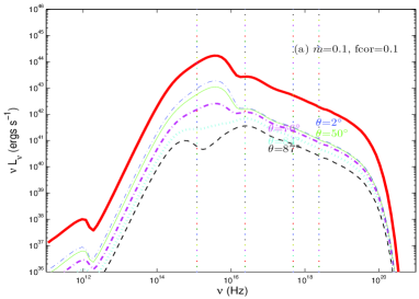
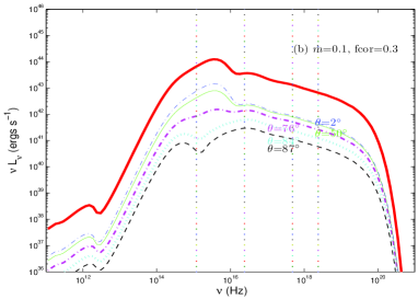
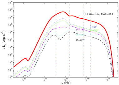
Figure 1: Spectra of the four disc-corona accretion models with different values of parameters $\dot{m}$ and $f_{\rm cor}$ in four plots, model (a): $\dot{m}=0.1$ and $f_{\rm cor}=0.1$, model (b): $\dot{m}=0.1$ and $f_{\rm cor}=0.3$, model (c): $\dot{m}=0.5$ and $f_{\rm cor}=0.06$, and model (d): $\dot{m}=0.5$ and $f_{\rm cor}=0.1$. For each model, we plot the spectra observed at different angles (the dashed lines in different colors). The emergent spectra viewed at $\theta=87^{\circ},84^{\circ},76^{\circ},50^{\circ}$, and $2^{\circ}$, are shown with black dashed, cyan dotted, magenta dash-dotted, green thin solid, and blue thin dash-dotted lines, respectively. The corresponding value of $\theta$ is denoted near each spectrum. The red thick solid lines are the spectra integrated over all directions ($\mu=0-1$). The four vertical dotted lines represent the four typical frequencies corresponding to $2500\rm\AA$, 0.1 keV, 2 keV, and 10 keV, respectively.

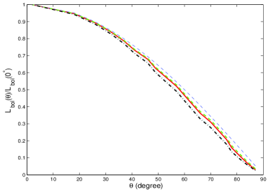
Figure 2: The observed bolometric luminosity varies with the viewing angle. The red solid, green dashed, cyan dotted, and black dash-dotted lines correspond to the four models (a)-(d) respectively. The blue thin dashed line indicates the relation of $L_{{\rm bol}}\propto\cos\theta$.

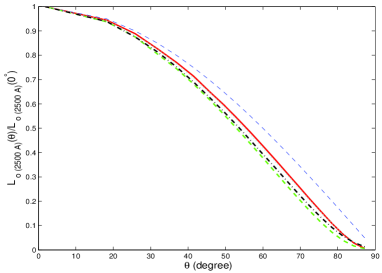
Figure 3: The spectral luminosity at optical/UV band($\lambda=2500{\rm\AA}$) varies with the viewing angle. The red solid, green dashed, cyan dotted, and black dash-dotted lines correspond to the four models (a)-(d) respectively. The blue thin dashed line represents the relation of $L_{\rm o}\propto\cos\theta$.

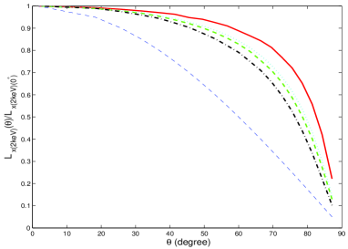
Figure 4: The spectral luminosity at X-ray band($E=2$ keV) varies with the viewing angle. The red solid, green dashed, cyan dotted, and black dash-dotted lines correspond to the four models (a)-(d) respectively. The blue thin dashed line represents the relation of $L_{\rm x}\propto\cos\theta$.

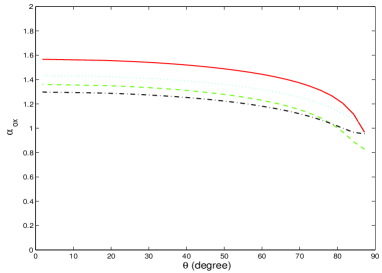
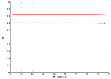
Figure 5: The optical/UV to X-ray spectral index, $\alpha_{\rm ox}$(upper panel), and the X-ray spectral index between 2 keV and 10 keV, $\alpha_{\rm x}$(lower panel), vary with the viewing angle. The red solid, green dashed, cyan dotted, and black dash-dotted lines correspond to the four models (a)-(d) respectively.

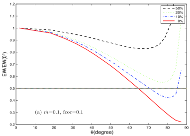
Figure 6: The equivalent width of the narrow Fe ${\rm K}{\alpha}$ line emitted from AGN varies with the viewing angle, which is calculated with model (a). The red solid line represents the case that all the line emission is radiated from the thin accretion disc. The black dashed, green dotted, and blue dash-dotted lines are the results of the cases that 50$\%$, 20$\%$, and 10$\%$ of the line luminosity contributed from the torus, respectively. The black dotted horizontal line represents the relative equivalent width being $0.5$.

5 Discussion

Solving the radiative transfer equation of the corona numerically, we obtain the cooling rate in the hot corona and the emergent spectrum of the accretion disc-corona system viewed at any specified angle. The calculations are carried out for four sets of model parameters, in which different accretion rate $\dot{m}$ and different ratio of the power dissipated in the corona $f_{\rm cor}$ are adopted, but all the other model parameters are fixed. Overall, the calculated spectra are sensitive to the values of the model parameters. For the models with same value of $f_{\rm cor}$ [compare Fig. 1(a) with 1(d)], the larger the accretion rate, the harder the spectra from the disc-corona accretion flow are. The X-ray emission predominantly originates from the inverse Compton scattering of the soft photons from the thin disc by the hot electrons in the corona. The larger the accretion rate, the more the soft photons are radiated from the disc, thus the emission in the lower energy band (i.e. optical/UV band) becomes relatively weaker while the high energy band (i.e. X-ray band) becomes relatively stronger, and the spectra are harder (see $\alpha_{\rm ox}$ in the left panel of Fig. 5). On the other hand, for the models with same value of $\dot{m}$ [compare Fig. 1(a) with 1(b), or Fig. 1(c) with 1(d)], the higher the ratio of the power dissipated in the corona, $f_{\rm cor}$, the harder the spectra from the disc-corona accretion flow are. We find that the electron temperature of the corona increases with $f_{\rm cor}$, which causes the Compton emission to be hard for the high $f_{\rm cor}$ cases.

It is found that the spectra of disc-corona system observed at different directions have the similar shapes in 2-10 keV X-ray band. The X-ray spectral index, $\alpha_{\rm x}$, remains almost unchanged for different viewing angle $\theta$ (see the lower panel of Figure 5). The X-ray emission mostly originates from the inverse Compton scattering of the soft photons radiated from the thin disc by the hot electrons in the corona. The inverse Compton scattered X-ray spectrum mainly depends on spectrum of the seed photons and the temperature of the hot electrons. Thus, the X-ray spectral index is not sensitive to the viewing direction. Comparing the values of $\alpha_{\rm x}$ for different models, we find that $\alpha_{\rm x}\approx 1.64$ for the case with $\dot{m}=0.1$ and $f_{\rm cor}=0.1$, while $\alpha_{\rm x}\approx 1.40$ for the case with $\dot{m}=0.5$ and $f_{\rm cor}=0.1$. This result seems inconsistent with the observed results and theoretical predictions in the previous works which claim the increasing $\alpha_{\rm x}$ with the Eddington ratio, $L_{\rm bol}/L_{\rm Edd}$ or accretion rate, $\dot{m}$ (e.g., see Fig. 4 in Cao, 2009). The reason is that we employ the same value of parameter, $f_{\rm cor}=0.1$, for these two models, which is inconsistent with the fact that the value of $f_{\rm cor}$ decreases with the accretion rate (e.g., see Fig. 1 in Cao, 2009). If we compare the results of the models (b) with (c), which adopt $f_{\rm cor}=0.3$ for the case with $\dot{m}=0.1$ and a smaller $f_{\rm cor}=0.06$ for the case with $\dot{m}=0.5$, we have $\alpha_{\rm x}\approx 1.43$ for the case with $\dot{m}=0.1$ and $f_{\rm cor}=0.3$ (see green line Figure 5), while $\alpha_{\rm x}\approx 1.62$ for the case with $\dot{m}=0.5$ and $f_{\rm cor}=0.06$ (see cyan line in Figure 5).

The main focus of this work is to explore the change of the emergent spectra from the disc-corona system viewed at different angles. In Figure 1, we find that the luminosity decreases with the increasing viewing angle $\theta$ with respect to the axis of the accretion disc. The detailed results of the observed bolometric luminosity are plotted in Figure 2, which shows that the bolometric luminosity is nearly proportional to $\mu$ ($\mu$=cos$\theta$). This is due to the area-projection effect. The change of the spectral shapes for different viewing angles is different between optical/UV and soft X-ray bands (see Figure 1). The observed spectral luminosity at a typical optical/UV band of $2500{\rm\AA}$ decreases with $\theta$ (see Figure 3). It decreases more rapidly than $\cos\theta$-relation. The blackbody emission from the thin disc is partly absorbed in the corona. For the optical/UV emission from the disc, the specific intensity of the photons from the upper surface of the corona, $I_{\nu}\sim I_{\nu,0}\exp({-\tau_{0}/\mu})$, where $I_{\nu,0}$ is the specific intensity of the photons injected in the lower surface of the corona, and $\tau_{0}$ is the vertical optical depth of the corona. Thus, the observed spectral luminosity at optical/UV band is proportion to $\mu\exp({-\tau_{0}/\mu})$, which decreases more quickly with $\theta$ than $\cos\theta$-relation. On the other hand, although the X-ray spectral shape remains unchanged for different $\theta$, the observed spectral luminosity at 2 keV decreases with $\theta$ (see Figure 4). It decreases more slowly than $\cos\theta$-relation.

The narrow 6.4 KeV Fe K$\alpha$ lines are ubiquity in AGNs. Although its origin is still uncertain, it was suggested that they may probably originate from the distant molecular cloud (torus), the outer accretion disc or/and the broad-line region (BLR). The BLR origin is ruled out by the fact that no correlation between the Fe K$\alpha$ core width and the BLR line (i.e., H$\beta$) width (Nandra, 2006). The emitted narrow 6.4 KeV line are found to show different properties for different types of AGN. The line luminosities of the narrow 6.4 KeV Fe K$\alpha$ line from type ${\rm I}$ AGNs are much stronger than those from type ${\rm II}$ AGNs at the same X-ray continuum luminosity. Compiling 89 Seyfert galaxies and using [O IV] emission to estimate the intrinsic luminosity of the sources, Liu & Wang (2010) found that the Fe K$\alpha$ line luminosities of Compton-thin Seyfert 2 galaxies are in average 2.9 times weaker than their Seyfert 1 counterparts. Ricci et al. (2014) found that the Fe K$\alpha$ line luminosity is correlated with the 10-50 keV X-ray continuum luminosity either for Sy1s and Sy2s. The slopes of the correlations are almost same for these two types of the sources, but the Fe K$\alpha$ line luminosities of Sy1s are about twice of those for Sy2s at a given X-ray continuum luminosity.

It is believed that type 1 Seyfert galaxies are intrinsically same as type 2 Seyferts but viewed at different angles (Antonucci, 1993). We find that the observed systematical difference of EW of Fe K$\alpha$ emission lines between Sy1s and Sy2s can be attributed to the difference of the view angles(see Figure 6). Such EW difference can be reproduced by our model calculations, provided Sy1s are observed in nearly face-on direction and the average inclination angle of Sy2s $\sim 65^{\circ}$, which support the unification scheme of AGN. If a fraction of Fe line emission is contributed by the torus, a larger average inclination angle is required for Sy2s, which implies that the contribution from the torus should be much less than that from the disc.

No significant correlation is found between the spectral index $\alpha_{\rm ox}$ and the radio core dominance parameter $R$, which is believed to be an indicator of the viewing angle (Runnoe, Shang, & Brotherton, 2013). Our results show that the spectral index $\alpha_{\rm ox}$ is weakly dependent on the inclination angle (see Figure 5). This is not surprising, because there is a strong correlation between $\alpha_{\rm ox}$ and optical luminosity/Eddington ratio (e.g., Vignali, Brandt, & Schneider, 2003; Grupe et al., 2010; Lusso et al., 2010). This correlation may smear out any possible correlation between $\alpha_{\rm ox}$ and inclination angle for a normal AGN sample. We suggest that the investigation on $\alpha_{\rm ox}$ and inclination angle relation should be carried out with a sample of AGNs in the narrow range of Eddington ratio/luminosity.

In the standard unification model of AGNs, the different observation properties of different types of AGN, such as, different continuum spectral shape and broad emission lines, can be explained by their different inclination angles of the black hole accretion flow and the surrounding torus. We show in this work that the emission spectra emitted from the accretion flow of a black hole are anisotropic along the different viewing angles, which is consistent with the area-projection effect in the bolometric luminosity, but very different in the other characteristics of SED, i.e., the spectral luminosities in the optical/UV band and the X-ray band. Our calculations of accretion disc-corona spectra may provide more precise orientation effect correction in predicting the intrinsic luminosity functions of AGN sources from the observed luminosities at certain band. Recently, the effect of anistropic radiation from the accretion discs on the luminosity function derived from an AGN sample was evaluated by DiPompeo et al. (2014), and they found that the bright end of the luminosity function may be overestimated by a factor of $\sim 2$ without considering this effect. A simple $\cos\theta$-dependent specific intensity from a bare accretion disc is used in their estimates. Our present detailed calculations of the disc corona spectra as functions of the viewing angle can be incorporated in deriving the intrinsic AGN luminosity.

The calculations of the radiation transfer in the corona in this work are carried out in Newtonian frame. A general relativistic accretion corona model is required for direct modeling the observed spectra of AGN. The calculations in this work can be easily expanded for the accretion discs surrounding Kerr black holes in general relativistic frame. This will be reported in our future work.

References

- Antonucci (1993) Antonucci R., 1993, ARA&A, 31, 473
- Balbus & Hawley (1991) Balbus S. A., Hawley J. F., 1991, ApJ, 376, 214
- Begelman & McKee (1990) Begelman M. C., McKee C. F., 1990, ApJ, 358, 375
- Bisnovatyi-Kogan & Lovelace (1997) Bisnovatyi-Kogan G. S., Lovelace R. V. E., 1997, ApJ, 486, L43
- Bisnovatyi-Kogan & Lovelace (2000) Bisnovatyi-Kogan G. S., Lovelace R. V. E., 2000, ApJ, 529, 978
- Cao (2004) Cao X., 2004, ApJ, 613, 716
- Cao (2009) Cao X., 2009, MNRAS, 394, 207
- Cao (2014) Cao X., 2014, ApJ, 783, 51
- Cao et al. (1998) Cao X., Jiang D. R., You J. H., Zhao J. L., 1998, A&A, 330, 464
- Coppi & Blandford (1990) Coppi P. S., Blandford R. D., 1990, MNRAS, 245, 453
- Di Matteo (1998) Di Matteo T., 1998, MNRAS, 299, L15
- Di Matteo, Celotti, & Fabian (1999) Di Matteo T., Celotti A., Fabian A. C., 1999, MNRAS, 304, 809
- DiPompeo et al. (2014) DiPompeo M. A., Myers A. D., Brotherton M. S., Runnoe J. C., Green R. F., 2014, ApJ, 787, 73
- Dove, Wilms, & Begelman (1997) Dove J. B., Wilms J., Begelman M. C., 1997, ApJ, 487, 747
- Dove et al. (1997) Dove J. B., Wilms J., Maisack M., Begelman M. C., 1997, ApJ, 487, 759
- Dullemond (1999) Dullemond C. P., 1999, A&A, 341, 936
- Esin et al. (1998) Esin A. A., Narayan R., Cui W., Grove J. E., Zhang S.-N., 1998, ApJ, 505, 854
- Galeev, Rosner, & Vaiana (1979) Galeev A. A., Rosner R., Vaiana G. S., 1979, ApJ, 229, 318
- Grupe et al. (2010) Grupe D., Komossa S., Leighly K. M., Page K. L., 2010, ApJS, 187, 64
- Haardt & Maraschi (1991) Haardt F., Maraschi L., 1991, ApJ, 380, L51
- Haardt & Maraschi (1993) Haardt F., Maraschi L., 1993, ApJ, 413, 507
- Hubeny et al. (2000) Hubeny I., Agol E., Blaes O., Krolik J. H., 2000, ApJ, 533, 710
- Kawaguchi, Shimura, & Mineshige (2001) Kawaguchi T., Shimura T., Mineshige S., 2001, ApJ, 546, 966
- Kawanaka, Kato, & Mineshige (2008) Kawanaka N., Kato Y., Mineshige S., 2008, PASJ, 60, 399
- Liu & Wang (2010) Liu T., Wang J.-X., 2010, ApJ, 725, 2381
- Liu, Mineshige, & Shibata (2002) Liu B. F., Mineshige S., Shibata K., 2002, ApJ, 572, L173
- Liu, Mineshige, & Ohsuga (2003) Liu B. F., Mineshige S., Ohsuga K., 2003, ApJ, 587, 571
- Lusso et al. (2010) Lusso E., et al., 2010, A&A, 512, A34
- Manmoto (2000) Manmoto T., 2000, ApJ, 534, 734
- Merloni & Fabian (2001) Merloni A., Fabian A. C., 2001, MNRAS, 328, 958
- Merloni & Fabian (2002) Merloni A., Fabian A. C., 2002, MNRAS, 332, 165
- Meyer & Meyer-Hofmeister (1994) Meyer F., Meyer-Hofmeister E., 1994, A&A, 288, 175
- Nakamura & Osaki (1993) Nakamura K., Osaki Y., 1993, PASJ, 45, 775
- Nandra (2006) Nandra K., 2006, MNRAS, 368, L62
- Narayan & Yi (1995) Narayan R., Yi I., 1995, ApJ, 452, 710
- Nayakshin & Dove (2001) Nayakshin S., Dove J. B., 2001, ApJ, 560, 885
- Nemmen & Brotherton (2010) Nemmen R. S., Brotherton M. S., 2010, MNRAS, 408, 1598
- Netzer (1987) Netzer H., 1987, MNRAS, 225, 55
- Pozdniakov, Sobol, & Siuniaev (1977) Pozdniakov L. A., Sobol I. M., Siuniaev R. A., 1977, SvA, 21, 708
- Ricci et al. (2014) Ricci C., Ueda Y., Paltani S., Ichikawa K., Gandhi P., Awaki H., 2014, MNRAS, 441, 3622
- Różańska & Czerny (2000) Różańska A., Czerny B., 2000, MNRAS, 316, 473
- Różańska & Czerny (2000) Różańska A., Czerny B., 2000, MNRAS, 316, 473
- Runnoe, Shang, & Brotherton (2013) Runnoe J. C., Shang Z., Brotherton M. S., 2013, MNRAS, 435, 3251
- Rybicki & Lightman (1986) Rybicki G. B., Lightman A. P., 1986, Radiative Processes in Astrophysics, by George B. Rybicki, Alan P. Lightman, pp. 400. ISBN 0-471-82759-2. Wiley-VCH , June 1986.
- Svensson & Zdziarski (1994) Svensson R., Zdziarski A. A., 1994, ApJ, 436, 599
- Vignali, Brandt, & Schneider (2003) Vignali C., Brandt W. N., Schneider D. P., 2003, AJ, 125, 433
- Witt, Czerny, & Zycki (1997) Witt H. J., Czerny B., Zycki P. T., 1997, MNRAS, 286, 848
- Wu et al. (2013) Wu Q., Cao X., Ho L. C., Wang D.-X., 2013, ApJ, 770, 31
- Xu (2013) Xu Y.-D., 2013, ApJ, 763, 75
- Xu (2013) Xu Y.-D., 2013, ApJ, 763, 75
- You, Cao, & Yuan (2012) You B., Cao X., Yuan Y.-F., 2012, ApJ, 761, 109
- Zdziarski et al. (2011) Zdziarski A. A., Skinner G. K., Pooley G. G., Lubiński P., 2011, MNRAS, 416, 1324
- Zhang (2005) Zhang S. N., 2005, ApJ, 618, L79
- Zycki, Collin-Souffrin, & Czerny (1995) Zycki P. T., Collin-Souffrin S., Czerny B., 1995, MNRAS, 277, 70