Supervised LogEuclidean Metric Learning
for Symmetric Positive Definite Matrices

Abstract

Metric learning has been shown to be highly effective to improve the performance of nearest neighbor classification. In this paper, we address the problem of metric learning for symmetric positive definite (SPD) matrices such as covariance matrices, which arise in many real-world applications. Naively using standard Mahalanobis metric learning methods under the Euclidean geometry for SPD matrices is not appropriate, because the difference of SPD matrices can be a non-SPD matrix and thus the obtained solution can be uninterpretable. To cope with this problem, we propose to use a properly parameterized LogEuclidean distance and optimize the metric with respect to kernel-target alignment, which is a supervised criterion for kernel learning. Then the resulting non-trivial optimization problem is solved by utilizing the Riemannian geometry. Finally, we experimentally demonstrate the usefulness of our LogEuclidean metric learning algorithm on real-world classification tasks for EEG signals and texture patches.

1 Introduction

Defining a distance to compare data points is an important problem occurring in many machine learning tasks. For instance, in classification, the nearest neighbor method Cover & Hart (1967) is equipped with a distance to identify the nearest neighbors. The performance of such a classifier highly depends on the quality of the equipped distance, and hence automatically finding a relevant distance from data has been the aim of many metric learning algorithms. So far, various methods have been developed for learning Mahalanobis distances in the Euclidean setting, and such metric learning methods have been successfully applied to diverse real-world problems including music recommendation Lim et al. (2013), face recognition Lu et al. (2012), image classification Mensink et al. (2012), link prediction in networks Shaw et al. (2011) and bioinformatics Wang et al. (2012). For the survey of recent advances, issues and perspectives in metric learning, see Bellet et al. (2013).

Classical metric learning approaches focused on an Euclidean setting which do not apply to complex or structured objects. Recently, metric learning for complex objects such as histograms Cuturi & Avis (2014); Kedem et al. (2012), binary codes Norouzi et al. (2012) and strings Bellet et al. (2011) have been actively explored, to which the Euclidean distance is not relevant. However, to the best of our knowledge, metric learning for symmetric positive definite (SPD) matrices has not been investigated thoroughly. Learning from SPD matrices, particularly from covariance matrices, arises in a number of important classification tasks such as brain imaging Arsigny et al. (2006); Dryden et al. (2009), brain-computer interfaces Barachant et al. (2010, 2013), pedestrian detection Tuzel et al. (2008) and texture classification Tuzel et al. (2006); Tou et al. (2009). In these applications, covariance matrices are either extracted from a physical model of the studied phenomenon (for diffusion tensor imaging) or as an empirical estimator from observations (for signal processing and computer-vision tasks). The purpose of this paper is to investigate metric learning for SPD matrices to boost the classification performance.

SPD matrices belong to an Euclidean space. For example, $2\times 2$ SPD matrix $A$ can be written as ${A=\left[\begin{array}[]{cc}a&b\\ b&c\end{array}\right]}$ with ${ac-b^{2}>0}$, $a>0$ and $c>0$. Then symmetric matrices can be represented as points in $\mathbb{R}^{3}$ and the constraints can be plotted as a cone, inside which SPD matrices lie strictly (see Fig. 1). A straightforward approach for learning a metric in this space would be to simply use the Euclidean distance $\delta_{e}$:

$$\delta_{e}(A,B) =\lVert A-B\rVert_{\mathcal{F}},$$ (1)

where $\lVert\cdot\rVert_{\mathcal{F}}$ denotes the Frobenius norm. The Euclidean geometry of symmetric matrices implies that distances are computed along straight lines according to $\delta_{e}$ (see Fig. 1 again).

Figure 1: Comparison between Euclidean (straight dashed lines) and Riemannian (curved solid lines) distances measured between points of the space $\mathcal{P}_{2}$.

However, the Euclidean geometry for averaging SPD matrices can result in a swelling effect Arsigny et al. (2007), i.e., the determinant of the average can be bigger than the determinant of each matrix. As also remarked in Fletcher & Joshi (2004) and illustrated in Fig. 1, this geometry creates a non-complete space, meaning that interpolation of SPD matrices is possible, but extrapolation can produce indefinite matrices. Hence, the swelling effect and the non-completeness of the space can result in uninterpretable solutions.

To avoid this problem, we use a more natural metric to compare SPD matrices, namely, the LogEuclidean distance $\delta_{l}$:

$$\delta_{l}(A,B)=\lVert\log\left(A\right)-\log\left(B\right)\rVert_{\mathcal{F}},$$ (2)

where $\log(\cdot)$ stands for the matrix logarithm. The LogEuclidean metric (and the derived distance and kernel) has been used in the literature Arsigny et al. (2006); Barachant et al. (2013), but its parameterization remained underestimated until recently Yger (2013). In this paper, we propose a supervised approach to learning the LogEuclidean metric. More specifically, we formulate our LogEuclidean metric learning problem as the kernel-target alignment problem Cristianini et al. (2001); Cortes et al. (2012), and solve the non-trivial optimization problem using the Riemannian geometry for SPD matrices. Through experiments on signal processing and computer vision applications, we demonstrate the efficacy of our proposed metric learning method.

2 Proposed approach

In this section, we describe our proposed metric learning method.

2.1 Formulation of metric learning under LogEuclidean distance

Let $\mathcal{S}_{d}$ be the set of real symmetric matrices of size $d\times d$. A matrix $A$ is said to be positive-definite ($A\succ 0$) if ${x^{\top}Ax>0}$ for all non-zero $x\in\mathbb{R}^{d}$, and the set of $d\times d$ SPD matrices is denoted by $\mathcal{P}_{d}$.

To learn a metric, we need to parameterize a distance. In this paper, following Bhatia (2009), we focus on the congruent transform, i.e., for any $A,G\in\mathcal{P}_{d}$,

$$\begin{cases}\quad\quad\quad\mathcal{P}_{d}\mapsto\quad\mathcal{P}_{d}\\ \Gamma_{G^{-\frac{1}{2}}}:A\to G^{-\frac{1}{2}}AG^{-\frac{1}{2}}.\end{cases}$$

Thus, the LogEuclidean distance (2) is parameterized using $G\in\mathcal{P}_{d}$ as

$$\delta_{l}^{G}(A,B) =\delta_{l}\left(\Gamma_{G^{-\frac{1}{2}}}(A),\Gamma_{G^{-\frac{1}{2}}}(B)\right)$$ (3)

$$=\lVert\log\left(G^{-\frac{1}{2}}AG^{-\frac{1}{2}}\right)-\log\left(G^{-\frac{1}{2}}BG^{-\frac{1}{2}}\right)\rVert_{\mathcal{F}}.$$

Our goal is to learn the parameter matrix $G$ from a set of $n$ training samples,

$$\{(X_{i},y_{i})|X_{i}\in\mathcal{P}_{d},y_{i}\in\{+1,-1\}\}_{i=1}^{n},$$

so that the performance of the nearest neighbor classifier on $\mathcal{P}_{d}$ is maximally enhanced.

$G$ was implicitly chosen as the identity matrix in Arsigny et al. (2006), while $G$ was heuristically chosen as the Riemannian mean of training samples in Barachant et al. (2013) and Yger (2013). Although these choices sound reasonable, we argue that they are sub-optimal when $\delta_{l}^{G}$ is used for nearest neighbor classification. Our aim is to find the optimal $G$ in terms of classification performance.

2.2 Metric learning with kernel-target alignment

For metric learning, we employ the (centered) kernel target alignment (KTA) criterion Cristianini et al. (2001); Cortes et al. (2012):

$$\mathcal{A}(K,K^{\star})=\frac{\langle UKU,UK^{\star}Umissing\rangle_{\mathcal{F}}}{\lVert UKU\rVert_{\mathcal{F}}\lVert UK^{\star}U\rVert_{\mathcal{F}}},$$

where $K$ is a matrix to be aligned, $K^{\star}=yy^{\operatorname{{}^{\mathrm{T}}}}$ is a target matrix, $y=(y_{1},\ldots,y_{n})^{\operatorname{{}^{\mathrm{T}}}}\in\mathbb{R}^{n}$, $U=\mathbb{I}_{d}-\frac{1_{d}1_{d}^{\top}}{d}$ is the centering matrix, $\mathbb{I}_{d}$ is the identity matrix of size $d\times d$, and $1_{d}$ is the $d$-dimensional vector with all ones. For simplicity, we suppose that $y$ is centered, i.e., $Uyy^{T}U\to yy^{T}$ below.

Let $k_{G}\left(X,X^{\prime}\right)$ be the LogEuclidean metric, from which the LogEuclidean distance (3) is derived:

$$k_{G}\left(X,X^{\prime}\right) =\operatorname{Tr}\left(\log\left(G^{-\frac{1}{2}}XG^{-\frac{1}{2}}\right)\log\left(G^{-\frac{1}{2}}X^{\prime}G^{-\frac{1}{2}}\right)\right),$$

where $X,X^{\prime},G\in\mathcal{P}_{d}$. Let $h(G)$ be the gram matrix for $k_{G}$:

$$h_{ij}(G)=k_{G}(X_{i},X_{j}).$$

Then our metric learning problem is formulated as

$$\max_{G\in\mathcal{P}_{d}}f\left(G\right),$$ (4)

where

$$f\left(G\right)=\mathcal{A}(h(G),yy\operatorname{{}^{\mathrm{T}}})=\frac{\langle Uh(G)U,yy\operatorname{{}^{\mathrm{T}}}missing\rangle_{\mathcal{F}}}{\lVert Uh(G)U\rVert_{\mathcal{F}}}.$$ (5)

A naive approach to solving the above optimization problem would be the projected gradient method, i.e., iteratively performing gradient ascent over $f(G)$ and projection of the updated solution back onto $\mathcal{P}_{d}$. However, since $\mathcal{P}_{d}$ is an open set (the strict interior of the cone is a set of SPD matrices, see Fig. 1 again), projection does not always exist. To cope with this problem, we introduce a more sophisticated approach based on the Riemannian geometry below.

2.3 Riemanian Gradient Optimization

Considering $\mathcal{P}_{d}$ as a Riemannian manifold provides us useful tools for solving our optimization problem. A basic optimization algorithm on the Riemannian manifold is the geodesic gradient descent, which optimizes the objective function along the geodesic computed from the Riemannian gradient $\text{grad}_{G}f(G)$. For optimization problem (4), the geodesic from $G_{t}$ to $G_{t+1}$ is given by

$$G_{t+1}= G_{t}^{\frac{1}{2}}\exp\left(\eta G_{t}^{-\frac{1}{2}}\text{grad}_{G_{t}}f(G_{t})G_{t}^{-\frac{1}{2}}\right)G_{t}^{\frac{1}{2}},$$ (6)

where $\eta\geq 0$ is the step size and $\exp(.)$ denotes the matrix exponential. Below, we explain how the above formula was derived.

As stated in Bhatia (2009), $\mathcal{P}_{d}$ is an open subset of the ambient Euclidean space of $d\times d$ symmetric matrices $\mathcal{S}_{d}$. As such, it is an instance of an embedded sub-manifold of $\mathcal{S}_{d}$ and so it is a differentiable manifold of dimension $d\left(d+1\right)/2$. From this structure of differential manifolds, we can derive the notion of tangent space $T_{G}\mathcal{P}_{d}$ at each point $G\in\mathcal{P}_{d}$. In general, tangent spaces are identified with subspaces of the ambient space. In the current setup, as $\mathcal{P}_{d}$ is an open sub-manifold, we identify the tangent space at $G$ as $T_{G}\mathcal{P}_{d}=\mathcal{S}_{d}$, the space of symmetric matrices of size $d\times d$.

Then, in order to turn this differential manifold into a Riemannian manifold, we need to equip its tangent spaces with a metric. One choice of metric (leading to a complete Riemannian manifold) is the affine-invariant metric, which, for $S_{A},S_{B}\in T_{G}\mathcal{P}_{d}$, is defined as:

$$\left\langle S_{A},S_{B}\right\rangle_{G}=\operatorname{Tr}\left(G^{-1}S_{A}G^{-1}S_{B}\right).$$ (7)

Note that a Riemannian gradient (that is used by first-order Riemannian optimization methods) is defined with respect to a given tangent space. Then, in order to be coherent with the metric of the tangent space (defined in Eq. (7)), $\text{grad}_{G}f(G)$, the Riemannian gradient at $G$ can be obtained from the Euclidean gradient $\nabla f$ as

$$\text{grad}_{G}f(G) =G\text{sym}(\nabla f(G))G.$$

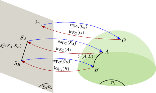
Figure 2: Mappings between the manifold of positive definite matrices and the tangent plane at the point $G$. As stated in Th. 2 $\delta_{e}^{G}$, the Euclidean distance in $T_{G}\mathcal{P}_{d}$ and the Riemannian distance $\delta_{r}$ are related but not equal in general.

As detailed in Appendix A.1, the Euclidean gradient $\nabla f\left(G\right)$ can be obtained as

$$\nabla f\left(G\right) =\sum_{ij}Z_{ij}(G)\nabla h_{ij}\left(G\right),$$

where

$$Z(G) =U\left(\frac{yy\operatorname{{}^{\mathrm{T}}}}{\lVert Uh(G)U\rVert_{\mathcal{F}}}-\frac{f\left(G\right)Uh\left(G\right)U}{\lVert Uh(G)U\rVert_{\mathcal{F}}^{2}}\right)U,$$

$$\nabla h_{ij}\left(G\right) =X_{i}^{-\frac{1}{2}}\left(DQ_{i}(G)\left[\text{sym}\left(A_{ij}\right)\right]\right)X_{i}^{-\frac{1}{2}}$$

$$\phantom{=}+X_{j}^{-\frac{1}{2}}\left(DQ_{j}(G)\left[\text{sym}\left(A_{ji}\right)\right]\right)X_{j}^{-\frac{1}{2}},$$

$$Q_{i}(G) =\log\left(X_{i}^{-\frac{1}{2}}GX_{i}^{-\frac{1}{2}}\right),$$

$$A_{ij} =X_{i}^{\frac{1}{2}}X_{j}^{-\frac{1}{2}}Q_{j}(G)X_{j}^{\frac{1}{2}}X_{i}^{-\frac{1}{2}},$$

$$\text{sym}\left(A\right) =\frac{A+A\operatorname{{}^{\mathrm{T}}}}{2},$$

where $Df\left(G\right)\left[\dot{G}\right]$ is the directional derivative of $f\left(G\right)$ in the direction $\dot{G}$. To our knowledge, there is no closed-form formula for computing the directional derivatives $DQ_{i}(G)\left[\text{sym}\left(A_{ij}\right)\right]$ and $DQ_{j}(G)\left[\text{sym}\left(A_{ji}\right)\right]$. However, we can numerically evaluate them, as shown in Boumal & Absil (2011) and Al-Mohy & Higham (2009).

Then any displacement in a tangent space $T_{G}\mathcal{P}_{d}$ can be mapped back on the manifold (and vice versa) using the reciprocal logarithmic and exponential mappings (see Fig. 2). Any symmetric matrix $S_{A}$ belonging to $T_{G}\mathcal{P}_{d}$, the tangent space at $G$, can be mapped on $\mathcal{P}_{d}$ (with the reciprocal operation) as

$$A= \exp_{G}\left(S_{A}\right)=G^{\frac{1}{2}}\exp\left(G^{-\frac{1}{2}}S_{A}G^{-\frac{1}{2}}\right)G^{\frac{1}{2}},$$ (8)

$$S_{A}= \log_{G}\left(A\right)=G^{\frac{1}{2}}\log\left(G^{-\frac{1}{2}}AG^{-\frac{1}{2}}\right)G^{\frac{1}{2}}.$$ (9)

These formula give the basic ingredients for implementing a geodesic gradient ascent method (as illustrated in Fig. 3) for our objective function. Indeed, from Eq. (8), the geodesic is given by

$$G_{t+1}= \exp_{G_{t}}\left(\eta\text{grad}_{G_{t}}f(G_{t})\right),$$

which leads to Eq. (6).

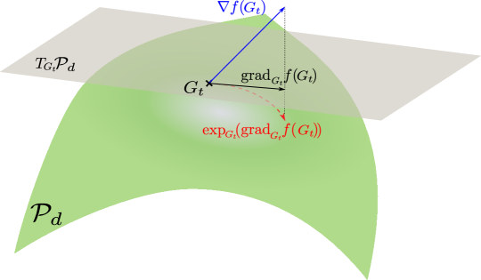
Figure 3: Graphical summary of a geodesic gradient descent method for a function $f$ on $\mathcal{P}_{d}$.

3 Discussions

In this section, we motivate the use of the LogEuclidean distance and compare it to other distances in $\mathcal{P}_{d}$.

3.1 Geometries on $\mathcal{P}_{d}$

Depending on the type of geometry chosen, there exist several choices of distances and divergences for comparing SPD matrices. As already discussed in literature Arsigny et al. (2006); Pennec et al. (2006); Dryden et al. (2009); Fletcher & Joshi (2004); Cherian et al. (2011), different tools come along with various implicit invariance properties and computational complexities.

As explained in Bhatia (2009), when using the geometry implied by the metric in Eq. 7, the distance between two SPD matrices $A$ and $B$ is computed along a curve (called the geodesic) and the associated affine-invariant Riemannian metric (AIRM) distance is defined as

$$\delta_{r}(A,B) =\lVert\log(A^{-\frac{1}{2}}BA^{-\frac{1}{2}})\rVert_{\mathcal{F}}$$ (10)

$$=\left(\sum_{i=1}^{d}\log^{2}\lambda_{i}\left(A,B\right)\right)^{\frac{1}{2}}$$

where $\lambda_{i}\left(A,B\right)$ are the eigenvalues of the pencil $(A,B)$.

As illustrated in Fig. 1, when using the Riemannian geometry, the space $\mathcal{P}_{d}$ becomes a complete manifold. As already stated in Arsigny et al. (2007), this distance is immune to the swelling effect. Thus, it could be a good candidate for distance metric learning for covariance matrices.

However, the AIRM distance comes along with an invariance to a class of congruent transforms Bhatia (2009) and it leads to the following isometry for any $M\in\mathcal{P}_{d}$:

$$\delta_{r}(\Gamma_{M}(A),\Gamma_{M}(B)) =\delta_{r}(A,B).$$ (11)

Hence, unlike the LogEuclidean distance, the AIRM distance is immune to the transform $\Gamma(.)$ and it can not be learned using our approach.

Apart from their difference in terms of invariance properties, it should be highlighted that the AIRM distance is not negative-definite and then, contrary to the LogEuclidean distance, cannot be used for defining positive-definite kernels on SPD matrices Haasdonk & Bahlmann (2004); Sra (2011); Barachant et al. (2013).

Using information geometry and extending divergences to the matrix case Cherian et al. (2011); Sra (2011, 2012), a symmetrized LogDeterminant divergence (also called the symmetrized Stein loss) can also be used. This divergence can be seen as an approximation of the AIRM distance and as such, there exist some bounds between the AIRM distance and this symmetrized divergence Sra (2011). Moreover, this divergence is invariant to the same transformation as the AIRM distance, but can lead under some conditions to a definite-positive kernel.

In this work, we look for a distance on SPD matrices tailored for classification. Due to the non-completeness of the space and the swelling effect, the Euclidean distance is not a valid candidate. Hence, the distances derived from Riemannian geometries (and their approximations) are more promising candidates, but in some cases, they are difficult to parametrize. Using the congruent transform $\Gamma_{G^{-\frac{1}{2}}}(.)$, it is possible to parametrize the LogEuclidean distance but not the AIRM distance nor the symmetrized Stein loss due to their invariance properties.

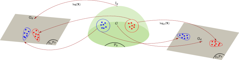
Figure 4: Illustration of the deformations implied by two mappings, respectively centered at the identity or at a point $G$

3.2 Interpretations of LogEuclidean metric learning

Compared to the Euclidean and AIRM distances, the LogEuclidean distance has several advantages: it is a Riemannian distance (immune to the swelling effect) and is easy to compute. In fact, using the fact that the mapping in Eq. (9) transforms matrices from the curved space $\mathcal{P}_{d}$ to the flat space $\mathcal{S}_{d}$, the LogEuclidean distance can be interpreted as the Euclidean distance between the matrices mapped into $\mathcal{S}_{d}$.

Interestingly, this LogEuclidean metric can be interpreted as the scalar product,

$$\langle S_{i},S_{j}\rangle_{G}=\operatorname{Tr}\left(G^{-\frac{1}{2}}S_{i}G^{-1}S_{j}G^{-\frac{1}{2}}\right),$$

in the tangent plane of $\mathcal{P}_{d}$ at the point $G$, with $S_{i}$ and $S_{j}$ the mapping around $G$ of $X_{i}$ and $X_{j}$ through the logarithmic map. Hence, according to the taxonomy developed in Bellet et al. (2013), since we optimize $G$ through a logarithmic mapping on a Riemannian manifold, our approach is an instance of non-linear similarity learning.

In this view, the parameter $G$ can be seen as the center of the tangent plane, and it has been empirically observed Yger (2013) that the choice of $G$ has a strong impact on the metric behaviour. So far, $G$ has been heuristically tuned using either the identity matrix or the Riemannian mean Moakher (2005); Jeuris et al. (2012) of data. However, as highlighted later, mapping a manifold onto a tangent space implies a deformation of the data. This deformation can either be harmful or beneficial to classification. By optimizing the choice of $G$ with respect to a discrimination criterion, we try to force the deformation to improve classification performance. As shown in Eq. (7), every tangent space is equipped with a different metric. Hence, choosing a new reference for a tangent space leads to choosing a new scalar product. In that sense, learning the reference point of a tangent space is equivalent to learning a metric.

The LogEuclidean metric is simply a scalar product (i.e., a linear kernel) applied to data mapped through a matrix logarithm. For this reason, it has sometimes been referred to as the LogEuclidean kernel Barachant et al. (2013); Yger (2013); Jayasumana et al. (2013). In this regard, the optimization of the LogEuclidean metric can also be interpreted as a kernel learning approach.

The use of the LogEuclidean distance can be interpreted as flattening the Riemannian manifold. As discussed below, such a mapping implies some deformations of the space of SPD matrices (see Fig. 4). Our approach can then be interpreted as finding the mapping such that the implied deformations benefit classification performance.

3.3 Geometrical motivation

The deformation implied by mapping points in a tangent space has been first stated as the exponential metric increasing (EMI) property in Bhatia (2009). It gives inequalities between the Riemannian distance $\delta_{r}$ and the Euclidean distance $\delta_{e}$ in the tangent space at the identity $\mathbb{I}_{d}$.

Theorem 1.

Bhatia (2009) For each pair of points $A$, $B$ in $\mathcal{P}_{d}$, we have

$$\delta_{r}(A,B)\geq\delta_{l}(A,B)=\|\log(A)-\log(B)\|_{\mathcal{F}}.$$

The equality occurs when $A$, $B$ and $\mathbb{I}_{d}$ belong to the same geodesic. This property, inherited from the non-positive curvature of $\mathcal{P}_{d}$, implies a deformation of the shapes when using the logarithmic map.

Using the properties of the bijection $\Gamma_{G^{-\frac{1}{2}}}(.)$ and with the notations in Eq. (7) and in Eq. (9), a corollary has been proposed in Yger (2013) which extends Theorem 1 to any tangent space:

Theorem 2.

(Yger, 2013) For any $A$, $B$ and $G$ in $\mathcal{P}_{d}$, with $\|\cdot\|_{G}$, the norm associated to the natural scalar product in $T_{G}\mathcal{P}_{d}$ satisfies

$$\delta_{r}(A,B)\geq\delta_{l}^{G}(A,B)=\|\log_{G}(A)-\log_{G}(B)\|_{G}.$$

Similarly to Theorem 1, the equality occurs when $A$, $B$ and $G$ belong to the same geodesic.

From these two theorems, as illustrated in Fig. 4, it follows that changing the reference point for centering the tangent space modifies how shapes are deformed once they are mapped in this tangent space. This motivates our metric learning approach.

4 Numerical experiments

In this section, we report experimental results.

4.1 Setup

Concerning the implementation of our approach, we employed a Riemannian trust-region Boumal & Absil (2011); Absil et al. (2009) . In practice, we use the following regularized optimization problem:

$$\begin{cases}\displaystyle\max_{G\in\mathcal{P}_{d}}f(G)\\ \text{s.t.~{}}\quad\delta_{r}(G_{0},G)\leq\epsilon\end{cases}$$

for some $G_{0}$. As we have not found any guarantee concerning the convexity or the geodesic-convexity Wiesel (2012) of the centered KTA, we decided to use the Riemannian mean Moakher (2005); Jeuris et al. (2012) as $G_{0}$. Below, we set $\epsilon=10$ for all datasets.

In our numerical experiments, we report accuracies on balanced datasets using a 1-nearest neighbor (1-NN) classifier equipped with different distances. Our baseline distances for the 1-NN classifier comprise the Euclidean distance $\delta_{e}$, the Riemannian distance $\delta_{r}$ and the LogEuclidean distance (parameterized by the identity matrix or the Riemannian mean of the training samples). We compare all these baseline distances to the LogEuclidean distance $\delta_{l}^{G}$ with parameter $G$ learned by our approach. In this section, when the reported results are averaged over several iterations (as in Tab. 1 and Tab. 3), we show when the improvement is significant using a bold font.

4.2 Toy dataset

First, in order to gain some insights on the behavior of our approach, we designed a simple experiment in which, the covariance matrices are generated as follows:

$$X =Q\text{diag}(\lambda_{1},\ldots,\lambda_{r},\mu_{1},\ldots,\mu_{r})Q^{\top}$$

$$\phantom{=}+V\text{diag}(|\epsilon_{1}|,\ldots,|\epsilon_{2r}|)V^{\top}$$

with $Q$ and $V$, two random orthonormal square matrices, and $\lambda_{i}\sim\mathcal{N}(5,0.2)$ or $\lambda_{i}\sim\mathcal{N}(4,0.1)$ respectively for the positive and negative classes and $\mu_{i}\sim\mathcal{U}([1,6])$ and $\epsilon_{i}\sim\mathcal{N}(0,1)$ independent of the class. The dataset is composed of $50$ samples in the training set and $500$ samples in the test set. It is re-sampled in order to repeat the experiment $10$ times and the results are reported in Tab. 1.

Table 1: Comparison of the mean accuracy of the LogEuclidean distance (parameterized by our method $G_{\text{KTA}}$) to other distances on a toy dataset with growing sizes of covariance matrices.

	LogEuclidean
size	$\mathbb{I}_{d}$	$\bar{X}$	$G_{\text{KTA}}$	$\delta_{r}$	$\delta_{e}$
6x6	77.50	77.58	84.78	77.66	82.76
8x8	77.46	77.44	86.78	77.42	83.32
16x16	75.58	75.62	89.56	75.48	85.78
20x20	77.06	77.10	90.96	77.16	87.16

In this simple experiment, as it was foreseeable, the Euclidean distance achieves good performances. Indeed, omitting the additive noise matrix, the data generation protocol only involves a fixed orthonormal matrix $Q$ for generating the matrices from both classes. Hence, the separation between the classes just becomes linear in terms of the eigenvalues of the covariance matrices. Interestingly, the Riemannian distances (except our approach) performs badly for all cases.

From this experiment, it is interesting to note that the proposed metric learning method helps the LogEuclidean distance to overcome its limitation.. Hence, the LogEuclidean distance with parameter learned by our proposed method is the best not only among the Riemannian distances but among all candidates. However, this toy experiment may be too simple for our applications and we test our methods on real-life datasets below.

4.3 Brain Computer-Interface

We tested our approach on Dataset 2a from the BCI Competition IV Naeem et al. (2006). The dataset consists of EEG signals (recorded from $22$ electrodes) on $9$ subjects who were asked to perform left hand, right hand, foot and tongue motor imagery Pfurtscheller & Neuper (2001) (i.e., EEG signals are recorded while the subject is only imagining the given limb movements without actually moving it).

Following the protocol described in Lotte & Guan (2011), we only used the EEG signals corresponding to the left and right hand. Hence, for every subject, we have $72$ trials (i.e. segments of signal) for each class in both training and testing. Moreover, we applied the same band-pass filtering ($[8-30]$ Hz) in order to pre-process the raw signals.

As shown in literature Barachant et al. (2010, 2013); Yger (2013), for motor imagery signals, the spatial covariance matrix of the trials is a very promising feature. Based on this observation, we extracted the covariance matrix between sensors (i.e., the spatial covariance matrix) from every filtered time segment (i.e., every example to be classified).

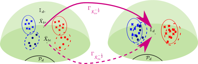
Figure 5: Illustration of the effect of whitening when the Riemannian mean of the data is non-stationary.

Although we could directly use our approach and try to classify samples, the performance would be poor since this dataset is known to show some non-stationarity between sessions. In order to cope with this problem, we employ an adaptive kernel formulation proposed in Barachant et al. (2013). This method cancels the non-stationarity in the data by whitening the covariance matrices in the training session and test session by subtracting the Riemannian mean of the training and test datasets, respectively. In practice, whitening is carried out by first applying the congruent transformation $\Gamma_{\bar{X}^{-\frac{1}{2}}}(\cdot)$, where $\bar{X}$ is the Riemannian mean of the data set. As illustrated in Fig. 5, this whitening process has the effect of spreading the covariance matrices from both training and test dataset around the identity matrix. For a dataset spread around $\bar{X}$, this has the effect of “transporting” the data on the manifold along the geodesic. For real-life applications, this whitening process can be criticized since it uses the test data. However, this can be carried out in a semi-supervised fashion by estimating $\bar{X}^{-\frac{1}{2}}$ during the calibration phase. Therefore, this process would still be practical in many applications.

As reported in Tab. 2, compared to other distances for handling covariance matrices, our proposed approach performs the best on $5$ subjects and is never the worst. On average over the subjects, we observe a significant gain by using an optimized reference point for the LogEuclidean distance.

Table 2: Comparison of the accuracy of the LogEuclidean distance (parameterized by our method $G_{\text{KTA}}$) to other distances for the classification of hand movements for $9$ subjects of the BCI Competition IV Dataset 2a.

	LogEuclidean
subject	$\mathbb{I}_{d}$	$G_{\text{KTA}}$	$\delta_{r}$	$\delta_{e}$
1	80.56	83.33	79.17	77.08
2	58.33	54.17	59.03	52.78
3	93.06	95.83	93.75	88.19
4	54.17	54.17	52.78	56.25
5	52.78	55.56	52.78	53.47
6	63.89	61.81	62.50	60.42
7	52.78	60.42	52.78	61.11
8	93.75	97.92	92.36	92.36
9	83.33	84.72	82.64	84.72
mean	70.29	71.99	69.75	69.60

4.4 Texture classification

As another example of real-world problems, we consider a subset of four textures (shown in Fig 6) of the Brodatz dataset Brodatz (1966). Similarly to the works of Mairal et al. (2009) and Yger & Rakotomamonjy (2011), we extracted $16\times 16$ patches from every texture. For every couple of textures, the training set composes patches from the left half of each texture and the test set composes patches from the right half. In every set, patches may overlap, but the training and test sets do not overlap each other.

Every method was trained on $50$ patches selected from the training set and tested on $300$ patches selected from the test set. Classification rates have been computed as the average of $50$ runs after re-sampling of the training and test sets.

(a) D2

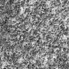
(b) D28

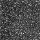
(c) D29

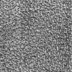
(d) D92

Figure 6: Selected textures from the Brodatz dataset

As proposed in Tou et al. (2009), we built covariance matrices using a bank of $8$ Gabor filters ($4$ angles and $2$ scales). Hence, each $16\times 16$ patch is transformed into a $8\times 8$ covariance matrix.

Table 3: Comparison of the mean accuracy of the LogEuclidean distance (parameterized by our method $G_{\text{KTA}}$) to other distances for classifying patches of texture taken from the Brodatz dataset.

	LogEuclidean
textures	$\mathbb{I}_{d}$	$\bar{X}$	$G_{\text{KTA}}$	$\delta_{r}$	$\delta_{e}$
D2 vs D28	86.37	86.58	88.39	86.31	63.53
D2 vs D29	75.5	75.33	76.69	75.14	64.03
D2 vs D92	74.88	74.68	76.71	74.33	68.05
D28 vs D29	75.5 0	75.33	76.69	75.14	64.03
D28 vs D92	74.88	74.68	76.71	74.33	68.05
D29 vs D92	83.68	83.53	85.83	83.48	65.93
mean	78.47	78.36	80.17	78.12	65.60

Tab. 3 summarizes the experiments on texture classification. First, it clearly shows the interest of using the Riemannian geometry. Indeed, for this data, the Euclidean distance performs poorly. Moreover, this experiment shows again that our supervised metric learning algorithm for choosing the reference of a LogEuclidean distance is effective.

5 Conclusion and perspectives

In this paper, we have introduced a novel approach for selecting a LogEuclidean metric. This approach is founded on theoretical observations about the distortion implied by a LogEuclidean metric. Then, we proposed to cast the problem of choosing a relevant metric as a kernel learning algorithm with a kernel target alignment criterion. We finally solved this problem using tools from the field of optimization on manifold and applied it to synthetic and real-world data.

Although we restricted ourselves to binary classification problems, the extension of our approach to multi-class problems  Ramona et al. (2012) is straightforward.

When huge datasets are involved, our optimization algorithm might not scale well. A stochastic setting on manifold Bonnabel (2013) could be a promising extention.

We only considered full-rank covariance matrices, but the extension of our approach to low-rank matrices is a challenging and interesting future work, since this corresponds to supervised feature extraction under the LogEuclidean metric. Exploration along this line of research would bridge the gap between our approach and the one proposed in Harandi et al. (2014).

Appendix A Appendix

In the appendix, we give more details about the derivation of the our cost function $f$ and we give the results of an extra numerical experiment on a toy dataset.

A.1 Gradient of f(G)

Deriving the cost function $f$ using the classical tricks of the trade of matrix derivation is not obvious (if not impossible). Indeed, this function is based on the matrix logarithm whose derivative is not simple to obtain.

To obtain the Euclidean gradient $\nabla f$ of the function $f$, we need $Df(X)[H]$, its directional derivative at a point $X$ and in a direction $H$, which is defined as:

$$Df(X)[H] =\lim_{h\to 0}\frac{f(X+hH)-f(X)}{h}$$

In order to obtain the gradient of $f$, we express its directional derivative. As the the gradient and the directional derivatives are linked with the following equality

$$Df\left(G\right)\left[\dot{G}\right] =\left\langle\nabla f\left(G\right),\dot{G}\right\rangle$$

we need the adjoint of the directional derivative in order to obtain $\nabla f\left(G\right)$.

Using standard properties of the directional derivatives, we formulate $Df\left(G\right)\left[\dot{G}\right]$ as :
 
 
 

$$Df\left(G\right)\left[\dot{G}\right] =\frac{\langle UDh\left(G\right)\left[\dot{G}\right]U,yy\operatorname{{}^{\mathrm{T}}}\rangle_{\mathcal{F}}\lVert Uh\left(G\right)U\rVert_{\mathcal{F}}-\langle Uh\left(G\right)U,yy\operatorname{{}^{\mathrm{T}}}\rangle_{\mathcal{F}}\langle\frac{Uh\left(G\right)U}{\lVert Uh\left(G\right)U\rVert_{\mathcal{F}}}UDh\left(G\right)\left[\dot{G}\right]U\rangle_{\mathcal{F}}}{\lVert Uh\left(G\right)U\rVert_{\mathcal{F}}^{2}}$$ (12)

$$= \left\langle Dh\left(G\right)\left[\dot{G}\right],\underbrace{U\left(\frac{yy\operatorname{{}^{\mathrm{T}}}}{\lVert Uh(G)U\rVert_{\mathcal{F}}}-\frac{f\left(G\right)Uh\left(G\right)U}{\lVert Uh(G)U\rVert_{\mathcal{F}}^{2}}\right)U}_{Z\left(G\right)}\right\rangle_{\mathcal{F}}$$ (13)

In Eq. 13, the core quantity to estimate is $Dh\left(G\right)$. Hopefully, the function $h\left(G\right)$ has already been studied in Boumal & Absil (2011). Using those results with the same convention ($\text{sym}\left(A\right)=\frac{A+A\operatorname{{}^{\mathrm{T}}}}{2}$), we have the gradient of $h_{ij}(G)$:

$$\nabla h_{ij}\left(G\right)= X_{i}^{-\frac{1}{2}}\left(D\log\left(X_{i}^{-\frac{1}{2}}GX_{i}^{-\frac{1}{2}}\right)\left[\text{sym}\left(X_{i}^{\frac{1}{2}}X_{j}^{-\frac{1}{2}}\log\left(X_{j}^{-\frac{1}{2}}GX_{j}^{-\frac{1}{2}}\right)X_{j}^{\frac{1}{2}}X_{i}^{-\frac{1}{2}}\right)\right]\right)X_{i}^{-\frac{1}{2}}$$ (14)

$$+X_{j}^{-\frac{1}{2}}\left(D\log\left(X_{j}^{-\frac{1}{2}}GX_{j}^{-\frac{1}{2}}\right)\left[\text{sym}\left(X_{j}^{-\frac{1}{2}}X_{i}^{\frac{1}{2}}\log\left(X_{i}^{-\frac{1}{2}}GX_{i}^{-\frac{1}{2}}\right)X_{i}^{-\frac{1}{2}}X_{j}^{\frac{1}{2}}\right)\right]\right)X_{j}^{-\frac{1}{2}}$$

Note that the gradient of $\nabla h_{ij}$ depends on the directionnal derivative of the matrix logarithm. To our knowledge, there is no closed-form formula of this directionnal derivative but is can be evaluated numerically using the algorithm in (Boumal & Absil, 2011; Al-Mohy & Higham, 2009).

Then, the Euclidean gradient of $f$ at $G$ is expressed with respect to the adjoint of $Dh\left(G\right)$:

$$\nabla f\left(G\right)=\left(Dh\left(G\right)\right)^{\star}\left[Z\left(G\right)\right].$$ (15)

Hence, after some algebra (detailed in the next section), we express the adjoint as :

$$\left\langle Z,Dh\left(G\right)\left[\dot{G}\right]\right\rangle_{\mathcal{F}}=\left\langle\overbrace{\sum_{ij}Z_{ij}\nabla h_{ij}\left(G\right)}^{\left(Dh\left(G\right)\right)^{\star}\left[Z\left(G\right)\right]},\dot{G}\right\rangle_{\mathcal{F}}.$$ (16)

To sum up, using Eq.14 and Eq.13, we have :

$$\nabla f\left(G\right)=\sum_{ij}Z_{ij}\nabla h_{ij}\left(G\right).$$ (17)

Note that, before solving our optimization problem on data, the validity of our Euclidean gradient formula has been numerically checked using the sanity checking tools provided in the Manopt toolbox by Boumal et al. (2014).

A.2 Adjoint of $Dh\left(G\right)$

In order to obtain the adjoint, using the decomposition over the canonical basis $\dot{G}=\sum_{k,l}\dot{G}_{kl}e_{k}e_{l}\operatorname{{}^{\mathrm{T}}}$, we write :

$$\left\langle Z,Dh\left(G\right)\left[\dot{G}\right]\right\rangle_{\mathcal{F}}$$ (18)

$$= \sum_{ij}Z_{ij}\left(Dh\left(G\right)\left[\dot{G}\right]\right)_{ij}$$ (19)

$$= \sum_{ij}\left\langle\nabla h_{ij}\left(G\right),\dot{G}\right\rangle_{\mathcal{F}}Z_{ij}$$ (20)

$$= \sum_{kl}\sum_{ij}\left\langle\nabla h_{ij}\left(G\right),Z_{ij}e_{k}e_{l}\operatorname{{}^{\mathrm{T}}}\right\rangle_{\mathcal{F}}\dot{G}_{kl}$$ (21)

$$= \sum_{kl}\left(\sum_{ij}Z_{ij}\nabla h_{ij}\left(G\right)\right)_{kl}\dot{G}_{kl}$$ (22)

$$= \left\langle\overbrace{\sum_{ij}Z_{ij}\nabla h_{ij}\left(G\right)}^{\left(Dh\left(G\right)\right)^{\star}\left[Z\left(G\right)\right]},\dot{G}\right\rangle_{\mathcal{F}}$$ (23)

A.3 Extra numerical experiments

We also report the numerical experiments of a simpler toy experiment. In this experiment, the data are generated in the same way :

$$X= Q\text{diag}(\lambda_{1},\ldots,\lambda_{r},\mu_{1},\ldots,\mu_{r})Q^{\top}$$

$$+ V\text{diag}(|\epsilon_{1}|,\ldots,|\epsilon_{2r}|)V^{\top}$$

with $Q$ and $V$, two random orthonormal square matrices, and $\lambda_{i}\sim\mathcal{N}(5,0.2)$ or $\lambda_{i}\sim\mathcal{N}(4,0.1)$ respectively for the positive and negative classes and $\mu_{i}\sim\mathcal{U}([1,3])$ and $\epsilon_{i}\sim\mathcal{N}(0,1)$ independently of the class.

The difference between those two experiments resides in the range in which the variables $\mu_{i}$ are sampled. Here, the range of the uniform distribution is smaller and this toy dataset becomes easier to classify.

The datasets were composed of $50$ examples in the training set and $500$ in test and every experiment was repeated $10$ times.

Table 4: Second experiment on a toy dataset with a weaker level of noise information.

	LogEuclidean
size	$\mathbb{I}_{d}$	$\bar{X}$	$G_{\text{KTA}}$	$\delta_{r}$	$\delta_{e}$
6x6	83.22	83.00	89.10	83.06	91.56
8x8	85.10	85.00	91.90	84.98	94.82
16x16	89.38	89.54	96.88	89.46	98.28
20x20	92.72	92.74	98.60	92.74	99.42

In this simple experiment, as in the other toy experiment, the Euclidean distance achieves the best performances for the same reasons.

Even if the Euclidean distance seems to be the most suited to those data, this toy experiment is interesting. Indeed, among the distances respecting the Riemannian geometry of the data (namely the LogEuclidean and Riemannian distances), the LogEuclidean distance parametrized by our approach performs the best. Optimizing the reference point $G$ (with respect to a KTA criterion) seems to diminish the impact of the uninformative variables $\mu$.

Note that in this experiment, the results of all approaches (including the Riemannian approaches) improves as the dimensionality grows. Contrary to the results reported in 1, in this experiment, the level of information is higher than the level of noise in the data. Hence, the more dimension we add, the easier it becomes to classify.

References

- Absil et al. (2009) Absil, P-A, Mahony, Robert, and Sepulchre, Rodolphe. Optimization algorithms on matrix manifolds. Princeton University Press, 2009.
- Al-Mohy & Higham (2009) Al-Mohy, Awad H and Higham, Nicholas J. Computing the fréchet derivative of the matrix exponential, with an application to condition number estimation. SIAM Journal on Matrix Analysis and Applications, 30(4):1639–1657, 2009.
- Arsigny et al. (2006) Arsigny, Vincent, Fillard, Pierre, Pennec, Xavier, and Ayache, Nicholas. Log-euclidean metrics for fast and simple calculus on diffusion tensors. Magnetic resonance in medicine, 56(2):411–421, 2006.
- Arsigny et al. (2007) Arsigny, Vincent, Fillard, Pierre, Pennec, Xavier, and Ayache, Nicholas. Geometric means in a novel vector space structure on symmetric positive-definite matrices. SIAM journal on matrix analysis and applications, 29(1):328–347, 2007.
- Barachant et al. (2010) Barachant, Alexandre, Bonnet, Stéphane, Congedo, Marco, and Jutten, Christian. Riemannian geometry applied to bci classification. In LVA/ICA, pp. 629–636, 2010.
- Barachant et al. (2013) Barachant, Alexandre, Bonnet, Stéphane, Congedo, Marco, and Jutten, Christian. Classification of covariance matrices using a riemannian-based kernel for bci applications. Neurocomputing, 112:172–178, 2013.
- Bellet et al. (2011) Bellet, Aurélien, Habrard, Amaury, and Sebban, Marc. Learning good edit similarities with generalization guarantees. In European Conference on Machine Learning and Principles and Practice of Knowledge Discovery in Databases (ECML/PKDD), pp. 188–203. Springer, 2011.
- Bellet et al. (2013) Bellet, Aurélien, Habrard, Amaury, and Sebban, Marc. A survey on metric learning for feature vectors and structured data. arXiv preprint arXiv:1306.6709, 2013.
- Bhatia (2009) Bhatia, Rajendra. Positive definite matrices. Princeton University Press, 2009.
- Bonnabel (2013) Bonnabel, Silvere. Stochastic gradient descent on riemannian manifolds. IEEE Transactions on Automatic Control, 58(9):2217–2229, Sept 2013.
- Boumal & Absil (2011) Boumal, Nicolas and Absil, P-A. Discrete regression methods on the cone of positive-definite matrices. In IEEE International Conference on Acoustics, Speech and Signal Processing (ICASSP), pp. 4232–4235. IEEE, 2011.
- Boumal et al. (2014) Boumal, Nicolas, Mishra, Bamdev, Absil, P-A, and Sepulchre, Rodolphe. Manopt, a matlab toolbox for optimization on manifolds. The Journal of Machine Learning Research (JMLR), 15(1):1455–1459, 2014.
- Brodatz (1966) Brodatz, Phil. Textures: a photographic album for artists and designers. Dover Pubns, 1966.
- Cherian et al. (2011) Cherian, Anoop, Sra, Suvrit, Banerjee, Arindam, and Papanikolopoulos, Nikolaos. Efficient similarity search for covariance matrices via the jensen-bregman logdet divergence. In IEEE International Conference on Computer Vision (ICCV), pp. 2399–2406. IEEE, 2011.
- Cortes et al. (2012) Cortes, Corinna, Mohri, Mehryar, and Rostamizadeh, Afshin. Algorithms for learning kernels based on centered alignment. The Journal of Machine Learning Research (JMLR), 13:795–828, 2012.
- Cover & Hart (1967) Cover, Thomas and Hart, Peter. Nearest neighbor pattern classification. IEEE Transactions on Information Theory, 13(1):21–27, 1967.
- Cristianini et al. (2001) Cristianini, Nello, Shawe-Taylor, John, Elisseeff, Andre, and Kandola, Jaz. On kernel target alignment. In NIPS, volume 2, pp. 4, 2001.
- Cuturi & Avis (2014) Cuturi, Marco and Avis, David. Ground metric learning. The Journal of Machine Learning Research (JMLR), 15(1):533–564, 2014.
- Dryden et al. (2009) Dryden, Ian L, Koloydenko, Alexey, and Zhou, Diwei. Non-euclidean statistics for covariance matrices, with applications to diffusion tensor imaging. The Annals of Applied Statistics, pp. 1102–1123, 2009.
- Fletcher & Joshi (2004) Fletcher, P Thomas and Joshi, Sarang. Principal geodesic analysis on symmetric spaces: Statistics of diffusion tensors. In Computer Vision and Mathematical Methods in Medical and Biomedical Image Analysis, pp. 87–98. Springer, 2004.
- Haasdonk & Bahlmann (2004) Haasdonk, Bernard and Bahlmann, Claus. Learning with distance substitution kernels. Pattern Recognition, pp. 220–227, 2004.
- Harandi et al. (2014) Harandi, Mehrtash, Salzmann, Mathieu, and Hartley, Richard. From manifold to manifold: geometry-aware dimensionality reduction for spd matrices. In Proceedings of the European Conference on Computer Vision (ECCV), pp. 17–32, 2014.
- Jayasumana et al. (2013) Jayasumana, Sadeep, Hartley, Richard, Salzmann, Mathieu, Li, Hongdong, and Harandi, Mehrtash. Kernel methods on the riemannian manifold of symmetric positive definite matrices. In IEEE Conference on Computer Vision and Pattern Recognition (CVPR), pp. 73–80, 2013.
- Jeuris et al. (2012) Jeuris, Ben, Vandebril, Raf, and Vandereycken, Bart. A survey and comparison of contemporary algorithms for computing the matrix geometric mean. Electronic Transactions on Numerical Analysis, 39:379–402, 2012.
- Kedem et al. (2012) Kedem, Dor, Tyree, Stephen, Sha, Fei, Lanckriet, Gert R, and Weinberger, Kilian Q. Non-linear metric learning. In NIPS, pp. 2573–2581, 2012.
- Lim et al. (2013) Lim, Daryl, Lanckriet, Gert, and McFee, Brian. Robust structural metric learning. In Proceedings of the 30th International Conference on Machine Learning (ICML), pp. 615–623, 2013.
- Lotte & Guan (2011) Lotte, Fabien and Guan, Cuntai. Regularizing common spatial patterns to improve bci designs: unified theory and new algorithms. IEEE Transactions on Biomedical Engineering, 58(2):355–362, 2011.
- Lu et al. (2012) Lu, Jiwen, Hu, Junlin, Zhou, Xiuzhuang, Shang, Yuanyuan, Tan, Yap-Peng, and Wang, Gang. Neighborhood repulsed metric learning for kinship verification. In IEEE Conference on Computer Vision and Pattern Recognition (CVPR), pp. 2594–2601, June 2012.
- Mairal et al. (2009) Mairal, Julien, Ponce, Jean, Sapiro, Guillermo, Zisserman, Andrew, and Bach, Francis. Supervised dictionary learning. In NIPS, 2009.
- Mensink et al. (2012) Mensink, Thomas, Verbeek, Jakob, Perronnin, Florent, and Csurka, Gabriela. Metric learning for large scale image classification: Generalizing to new classes at near-zero cost. In European Conference on Computer Vision (ECCV), pp. 488–501. Springer, 2012.
- Moakher (2005) Moakher, Maher. A differential geometric approach to the geometric mean of symmetric positive-definite matrices. SIAM Journal on Matrix Analysis and Applications, 26(3):735–747, 2005.
- Naeem et al. (2006) Naeem, M, Brunner, C, Leeb, R, Graimann, B, and Pfurtscheller, G. Seperability of four-class motor imagery data using independent components analysis. Journal of neural engineering, 3(3):208, 2006.
- Norouzi et al. (2012) Norouzi, Mohammad, Blei, David M, and Salakhutdinov, Ruslan R. Hamming distance metric learning. In NIPS, pp. 1061–1069, 2012.
- Pennec et al. (2006) Pennec, Xavier, Fillard, Pierre, and Ayache, Nicholas. A riemannian framework for tensor computing. International Journal of Computer Vision, 66(1):41–66, 2006.
- Pfurtscheller & Neuper (2001) Pfurtscheller, Gert and Neuper, Christa. Motor imagery and direct brain-computer communication. Proceedings of the IEEE, 89(7):1123–1134, 2001.
- Ramona et al. (2012) Ramona, Mathieu, Richard, Gaël, and David, Bertrand. Multiclass feature selection with kernel gram-matrix-based criteria. IEEE Transactions on Neural Networks and Learning Systems, 23(10):1611–1623, 2012.
- Shaw et al. (2011) Shaw, Blake, Huang, Bert, and Jebara, Tony. Learning a distance metric from a network. In NIPS, pp. 1899–1907, 2011.
- Sra (2011) Sra, Suvrit. Positive definite matrices and the s-divergence. arXiv preprint arXiv:1110.1773, 2011.
- Sra (2012) Sra, Suvrit. A new metric on the manifold of kernel matrices with application to matrix geometric means. In NIPS, pp. 144–152, 2012.
- Tou et al. (2009) Tou, Jing Yi, Tay, Yong Haur, and Lau, Phooi Yee. Gabor filters as feature images for covariance matrix on texture classification problem. In Advances in Neuro-Information Processing, pp. 745–751. Springer, 2009.
- Tuzel et al. (2006) Tuzel, Oncel, Porikli, Fatih, and Meer, Peter. Region covariance: A fast descriptor for detection and classification. In European Conference on Computer Vision (ECCV), pp. 589–600, 2006.
- Tuzel et al. (2008) Tuzel, Oncel, Porikli, Fatih, and Meer, Peter. Pedestrian detection via classification on riemannian manifolds. IEEE Transactions on Pattern Analysis and Machine Intelligence, 30(10):1713–1727, 2008.
- Wang et al. (2012) Wang, Jingyan, Gao, Xin, Wang, Quanquan, and Li, Yongping. Prodis-contshc: learning protein dissimilarity measures and hierarchical context coherently for protein-protein comparison in protein database retrieval. BMC bioinformatics, 13(Suppl 7):S2, 2012.
- Wiesel (2012) Wiesel, Ami. Geodesic convexity and covariance estimation. IEEE Transactions on Signal Processing, 60(12):6182–6189, 2012.
- Yger (2013) Yger, Florian. A review of kernels on covariance matrices for bci applications. In IEEE International Workshop on Machine Learning for Signal Processing (MLSP), pp. 1–6. IEEE, 2013.
- Yger & Rakotomamonjy (2011) Yger, Florian and Rakotomamonjy, Alain. Wavelet kernel learning. Pattern Recognition, 44(10):2614–2629, 2011.