Estimating the dark matter halo mass of our Milky Way using dynamical tracers

Abstract

The mass of the dark matter halo of the Milky Way can be estimated by fitting analytical models to the phase-space distribution of dynamical tracers. We test this approach using realistic mock stellar halos constructed from the Aquarius N-body simulations of dark matter halos in the $\Lambda$CDM cosmology. We extend the standard treatment to include a Navarro-Frenk-White (NFW) potential and use a maximum likelihood method to recover the parameters describing the simulated halos from the positions and velocities of their mock halo stars. We find that the estimate of halo mass is highly correlated with the estimate of halo concentration. The best-fit halo masses within the virial radius, $R_{200}$, are biased, ranging from a 40% underestimate to a 5% overestimate in the best case (when the tangential velocities of the tracers are included). There are several sources of bias. Deviations from dynamical equilibrium can potentially cause significant bias; deviations from spherical symmetry are relatively less important. Fits to stars at different galactocentric radii can give different mass estimates. By contrast, the model gives good constraints on the mass within the half-mass radius of tracers even when restricted to tracers within 60 kpc. The recovered velocity anisotropies of tracers, $\beta$, are biased systematically, but this does not affect other parameters if tangential velocity data are used as constraints.

1 Introduction

Our Milky Way (MW) galaxy provides a wealth of information on the physics of galaxy formation and the nature of the dark matter. This information can, in principle, be unlocked from studies of the positions, velocities and chemistry of stars in the Galaxy, its satellites and globular clusters, which can be observed with high precision.

Many inferences derived from the properties of the Milky Way (MW) depend on the precision and accuracy with which the mass of its dark matter halo can be estimated. An example is the much-publicised “too big to fail” problem, the apparent lack of MW satellite galaxies with central densities as high as those of the most massive dark matter subhalos predicted by $\mathrm{\Lambda}$CDM simulations of ‘Milky Way mass’ hosts (Boylan-Kolchin et al., 2011, 2012; Ferrero et al., 2012). In these simulations the number of massive subhalos depends strongly on the assumed MW halo mass and the problem disappears if the MW halo mass is sufficiently small ($\lower 3.22916pt\hbox{$\sim$}\hbox to0.0pt{\hss\raise 1.1625pt\hbox{$<$}}1\times 10^{12}$ M_⊙; Wang et al., 2012; Cautun et al., 2014).

Gravitational lensing is the most powerful method to determine the underlying dark matter distribution for large samples of distant galaxies (e.g. Bartelmann & Schneider, 2001; Mandelbaum et al., 2006; Li et al., 2009; Hilbert & White, 2010; Han et al., 2015). Our MW is, however, special because we are embedded in it, and there are many different ways of constraining the MW dark matter halo mass.

These methods include timing argument estimators (Kahn & Woltjer, 1959) calibrated against $N$-body simulations (Li & White, 2008); modeling of local cosmic expansion (Peñarrubia et al., 2014); the kinematics of bright satellites (Sales et al., 2007b, a; Barber et al., 2014; Cautun et al., 2014), particularly Leo I (Boylan-Kolchin et al., 2013) and the Magellanic Clouds (Busha et al., 2011; González et al., 2013); the kinematics of stellar streams (Newberg et al., 2010; Küpper et al., 2015), especially the Sagittarius stream (Law et al., 2005; Gibbons et al., 2014); measurements of the escape velocity using nearby high velocity stars, such as those from the RAVE survey (Smith et al., 2007; Piffl et al., 2014); and combinations of photometric and kinematic data such as Maser observations and terminal velocity curves (McMillan, 2011; Nesti & Salucci, 2013). Using high resolution hydrodynamical simulations and the line-of-sight velocity dispersion of tracers in the MW, Rashkov et al. (2013) found a heavy MW halo mass reported in some previous measurements of $M_{200}\approx 2\times 10^{12}\mathrm{M_{\odot}}$ is disfavoured.

Some authors have used large composite samples of objects assumed to be dynamical tracers in the halo, such as stars, globular clusters and planetary nebulae. For example, the halo circular velocity, $V_{\mathrm{circ}}$, may be inferred from the radial velocity dispersion of tracers, $\sigma_{r}(r)$, using the spherical Jeans equation. Such methods require the tracer velocity anisotropy and density profiles to be known or assumed. Battaglia et al. (2005) made use of a few hundred stars and globular clusters from 20 to 120 kpc; Xue et al. (2008) used 2401 BHB stars from SDSS/DR6 ranging from 20 to 60 kpc; Gnedin et al. (2010) used BHB and RR Lyrae stars ranging from 25 to 80 kpc; and Watkins et al. (2010) used 26 satellites within 300 kpc with tracer mass estimators, with the method further improved by Evans et al. (2011) and An et al. (2012). Most recently Kafle et al. (2012, 2014) used a few thousand BHB stars extending to 60 kpc and K-giants beyond 100 kpc.

Most measurements based on dynamical tracers involve assumptions about the tracer density profiles and velocity anisotropies. However, Wilkinson & Evans (1999) introduced a Bayesian likelihood analysis, based on fitting a model phase-space distribution function to the observed distances and velocities of tracers. In their analysis the tracer density profile and velocity anisotropy can be considered as free parameters of the distribution function, to be constrained together with parameters of the host halo such as its mass and characteristic scalelength. The sample of stars used by Wilkinson & Evans (1999) was small and their best-fit host halo mass for a truncated flat rotation curve model was $1.9_{-1.7}^{+3.6}\times 10^{12}$ M_⊙ (see also Sakamoto et al. 2003). More recently, Deason et al. (2012) used a few thousand BHB stars from SDSS up to $r\sim$50 kpc. Eadie et al. (2015) introduced a generalised Bayesian approach to deal with incomplete data, which avoids rewriting the distribution function when tangential velocities are not available.

Figure 1: Measured MW halo masses in the literature ($x$-axis), converted to $M_{200}$ and categorised by methodology ($y$-axis). Measurements using similar methods and/or tracer populations are plotted with the same colour. Categories include the timing argument estimator (black); a model of the local cosmic expansion (light grey); constraints from luminous MW satellites such as the Magellanic Clouds (magenta), Leo I(cyan), the orbits or radial velocity dispersion of other bright satellites (yellow) and their $V_{\mathrm{max}}$ distribution (light green); modelling of tidal streams (grey); high velocity stars from the RAVE survey (blue); combinations of maser observations and and the terminal velocity curve (pink); and (of most relevance to this work) dynamical modelling using large samples of dynamical tracers (red and green). Methods involving large samples of dynamical tracers are split into two categories, 1) those based on the radial velocity dispersion of tracers (green) and 2) those using model distribution function to constrain both halo properties and velocity anisotropies of tracers simultaneously (red). We have converted results to $M_{200}$ by assuming an NFW density profile and a common mass-concentration relation. 95% or 90% confidence intervals have been converted to 1$\sigma$ errors by assuming a Gaussian error distribution, except for Watkins et al. and measurements in the DF classification.

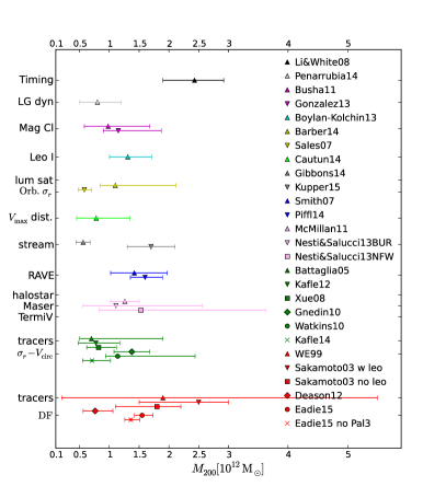
Fig. 1 summarises the results of these studies. The $x$-axis is the measured MW halo mass. We have converted results to $M_{200}$ by assuming an NFW density profile (Navarro et al., 1996a, 1997a) and using the mean halo concentration relation of Duffy et al. (2008) in cases where a value for concentration is not given in the original study. The measurements are grouped by methodology, indicated by colours and labeled along the $y$-axis. We group those methods that use large samples of dynamical tracers into two sets: 1) those based on the radial velocity dispersion of the tracers and spherical Jeans equation to infer the circular velocity and underlying potential; 2) those based on fitting to model distribution functions, which attempt to constrain both halo mass and the velocity anisotropy of the tracers simultaneously. Errorbars correspond to those quoted by the original authors; we have converted 90% or 95% confidence intervals to 1$\sigma$ errors assuming a Gaussian distribution, except for Watkins et al. and measurements in the DF classification. This is because Wilkinson & Evans (1999), Sakamoto et al. (2003), Watkins et al. (2010), and Deason et al. (2012) included other sources of model uncertainties beyond pure statistical errors in their measured masses, which makes their errors relatively large. For the generalised Bayesian approach of Eadie et al. (2015), we quote the 95% Bayesian confidence interval. Fig. 1 shows that existing measurements of the most likely MW halo mass differ by more than a factor of 2.5, even when similar methods are used, although apart from a few outliers, the estimates are statistically consistent.

Here we are particularly interested in methods such as that of Wilkinson & Evans (1999), which treat the spatial and dynamical properties of tracers as free parameters to be constrained under the assumption of theoretical phase-space distribution functions. The primary aim of this paper is to test the model distribution functions used in this approach. We extend the distribution function proposed by Wilkinson & Evans (1999) to one based on the NFW potential, and model the radial profiles of tracers with a more general double power-law functional form. The model function is then fit to the phase-space distribution of stars in realistic mock stellar halo catalogues constructed from the cosmological galactic halo simulations of the Aquarius project (Springel et al., 2008), to understand its reliability and possible violations to the underlying assumptions. Our results have implications that are not limited to the specific form of the distribution function that we test, but are applicable to the method itself.

This paper is structured as follows. The mock stellar halo catalogues are introduced in Section 2. Detailed descriptions of the model distribution function and the maximum likelihood approach are provided in Section 3. Our results are presented in Section 4, with detailed discussions of reliability and systematics in Section 5 and Section 6. We conclude in Section 7. Throughout this paper we adopt the cosmology of the Aquarius simulation series ($H_{0}=73~{}\mathrm{km~{}s^{-1}}~{}\mathrm{Mpc}^{-1}$, $\Omega_{\rm m}=0.25$, $\Omega_{\Lambda}=0.75$ and $n=1$).

2 Mock stellar halo catalogue

We use mock stellar halo catalogues constructed from the Aquarius N-body simulation suite (Springel et al., 2008) with the particle tagging method described by Cooper et al. (2010), to which we refer the reader for further details. In this section we summarise the most important features of these catalogues.

2.1 The Aquarius simulations

The Aquarius halos come from dark matter N-body simulations in a standard $\mathrm{\Lambda}$CDM cosmology. Cosmological parameters are those from the first year data of WMAP (Spergel et al., 2003). Our work uses the second highest resolution level of the Aquarius suite, which corresponds to a particle mass of $\sim 10^{4}h^{-1}$ M_⊙.

The simulation suite includes six dark matter halos with virial masses spanning the factor-of-two range of Milky Way observations discussed in the previous section. We have only used five out of the six halos for our analysis (labeled halo A to halo E according to the Aquarius convention). The halo we have not used (halo F) undergoes two major merger events at $z<0.6$, and is thus an unlikely host for a MW-like disc galaxy. We list in Table LABEL:tbl:parameters the host halo mass, $M_{200}$, and other properties of the five halos, which are taken from Navarro et al. (2010).

2.2 The galaxy formation and evolution model

The Durham semi-analytical galaxy formation model, GALFORM, has been used to post-process the Aquarius simulations, predicting the evolution of galaxies embedded in dark matter halos. To construct the mock stellar halo catalogues used in this paper, the version described by Font et al. (2011) was adopted. This model has several minor differences from the model of Bower et al. (2006), such that the Font et al. (2011) model matches better the observed luminosity function, luminosity-metallicity relation and radial distribution of MW satellites. The main changes are a more self-consistent calculation of the effects of the patronisation background and a higher chemical yield in supernovae feedback.

2.3 Particle tagging

The GALFORM model predicts the amount of stellar mass present in each dark matter halo in the simulation at each output time, as well as properties of stellar populations such as their total metallicity. However, GALFORM does not provide detailed information about how these stars are distributed in galaxies. The particle tagging method of Cooper et al. (2010) is a way to determine the six-dimensional spatial and velocity distribution of stars from dark matter only simulations, by associating newly-formed stars with tightly bound dark matter particles.

At each simulation snapshot, each newly formed stellar population predicted by GALFORM is assigned to the 1% most bound dark matter particles in its host dark matter halo. Each “tagged” dark matter particle then represents a fraction of a single stellar population, the age and metallicity of which are also known from GALFORM. Traced forward to the present day, these tagged particles give predictions for the observed luminosity functions and structural properties of MW and M31 satellites that match well to observations. Recently, Cooper et al. (2013) have applied this technique to large-scale cosmological simulations and have shown that it produces galactic surface brightness profiles that agree well with the outer regions of stacked galaxy profiles from SDSS.

Our study is based on tagged dark matter particles from accreted satellite galaxies. We ignore particles associated with in situ star formation in the central galaxy. Strictly, our results thus only apply in the case where most MW halo stars originate from accretion. This is supported by the data of Bell et al. (2008, 2010) although other work suggests that a certain fraction of the halo stars are contributed by in-situ star formation, especially close to the central galaxy ($r<30$ kpc) (see, e.g. Carollo et al., 2007; Carollo et al., 2010; Zolotov et al., 2010; Helmi et al., 2011). Ignoring the possible in-situ component is thus a weakness of our mock stellar halo catalogue. Nevertheless, our mock halo stars enable us to test and constrain the theoretical distribution function and, in practice, most of our conclusions (see Sec. 4 and Sec. 5) do not depend on whether the MW halo stars formed in-situ or were brought in by accretion.

Figure 2: The radial density profiles of stellar mass (red points and lines with errors) in the mock stellar halo catalogue of the five Aquarius halos. The errors are in most cases of comparable size to the symbols and are almost invisible. Dashed black curves are double power-law fits to the red data points obtained from a $\chi^{2}$ minimisation. Green dashed curves are the best-fit density profiles from the maximum likelihood method.

3 Methodology

In this section we discuss the theoretical context of our method for constraining dark matter halo properties using dynamical tracers and a maximum likelihood approach based on theoretical distribution functions. In Sec. 3.1, we describe how the phase-space distribution of the tracer population is modeled. Sec. 3.2 gives details about the explicit form of the distribution function. The likelihood function is introduced in Sec. 3.3. Finally, we describe how we weight tagged particles and how errors are estimated in Sec. 3.4. Our method follows that of Wilkinson & Evans (1999) but introduces significant modifications to the form of the dark matter halo potential and the assumed tracer density profile.

3.1 Phase-space distribution of Milky Way halo stars

The phase-space distribution function of tracers (e.g. stars) bound to a dark matter halo potential (binding energy $E>0$) can be described by the Eddington formula (Eddington, 1916). The simplest isotropic and spherically symmetric case is

$$F(E)=\frac{1}{\sqrt{8}\pi^{2}}\frac{\mathrm{d}}{\mathrm{d}E}\int_{\Phi(r_{\mathrm{max,t}})}^{E}\frac{\mathrm{d}\rho(r)}{\mathrm{d}\Phi(r)}\frac{\mathrm{d}\Phi(r)}{\sqrt{E-\Phi(r)}},$$ (1)

where the distribution function only depends on the binding energy per unit mass, $E=\Phi(r)-\frac{v^{2}}{2}$. $\Phi(r)$ and ${v^{2}}/{2}$ are the underlying dark matter halo potential and kinetic energy per unit mass of tracers. The integral goes from the potential at the tracer boundary to the binding energy of interest. Usually both the zero point of potential and tracer boundary, $r_{\mathrm{max,t}}$, are chosen at infinity, and thus $\Phi(r_{\mathrm{max,t}})=0$.

In reality the velocity distribution of tracers may be anisotropic and depend both on energy and angular momentum, $L$. In the simplest case, the distribution function is assumed to be separable:

$$F(E,L)=L^{-2\beta}f(E),$$ (2)

where the energy part, $f(E)$, is expressed as (Cuddeford, 1991)

$$\begin{split}f(E)=\frac{2^{\beta-3/2}}{\pi^{3/2}\Gamma(m-1/2+\beta)\Gamma(1-\beta)}\times\\ \frac{\mathrm{d}}{\mathrm{d}E}\int_{\Phi(r_{\mathrm{max,t}})}^{E}(E-\Phi)^{\beta-3/2+m}\frac{\mathrm{d}^{m}[r^{2\beta}\rho(r)]}{\mathrm{d}\Phi^{m}}\mathrm{d}\Phi\\ =\frac{2^{\beta-3/2}}{\pi^{3/2}\Gamma(m-1/2+\beta)\Gamma(1-\beta)}\times\\ \int_{\Phi(r_{\mathrm{max,t}})}^{E}(E-\Phi)^{\beta-3/2+m}\frac{\mathrm{d}^{m+1}[r^{2\beta}\rho(r)]}{\mathrm{d}\Phi^{m+1}}\mathrm{d}\Phi.\end{split}$$ (3)

Here $\beta$ is the velocity anisotropy parameter defined as

$$\beta=1-\frac{{\langle{v_{\theta}}\rangle}^{2}-{\langle v_{\theta}\rangle}^{2}+{\langle{v_{\phi}}^{2}\rangle}-{\langle v_{\phi}\rangle}^{2}}{2({\langle{v_{r}}^{2}\rangle}-{\langle v_{r}\rangle}^{2})},$$ (4)

with $v_{r}$, $v_{\theta}$ and $v_{\phi}$ being the radial and two tangential components of the velocity. The integer, $m$, is chosen to make the integral converge and depends on the value of $\beta$. In our analysis the parameter range of $\beta$ is $-0.5<\beta<1$ and $m=1$. $\beta>0$ represents radial orbits, while tangential orbits have $\beta<0$. $\beta=0$ corresponds to the isotropic velocity distribution.

In real observations, the tangential velocities of tracers are often unavailable. We thus test two different cases, in which i) only radial velocities are available and ii) both radial and tangential velocities are available. For case (i), the phase-space distribution in terms of radius, $r$, and radial velocity, $v_{r}$, is given by the integral over tangential velocity, $v_{t}=\sqrt{v_{\theta}^{2}+v_{\phi}^{2}}$, as

$$P(r,v_{r}|C)=\int L^{-2\beta}f(E)2\pi v_{t}\mathrm{d}v_{t},$$ (5)

where $C$ denotes a set of model parameters. With the Laplace transform, this can be written as

$$P(r,v_{r}|C)=\frac{1}{\sqrt{2}\pi r^{2\beta}}\int_{\Phi(r_{\mathrm{max,t}})}^{E_{r}}\frac{\mathrm{d}\Phi}{\sqrt{E_{r}-\Phi}}\frac{\mathrm{d}r^{2\beta}\rho(r)}{\mathrm{d}\Phi},$$ (6)

where $E_{r}=\Phi(r)-v_{r}^{2}/2$. All factors of $m$ cancel in the Laplace transform and hence Eqn. 6 does not depend on $m$. For case (ii), the distribution function is simply Eqn. 2, i.e.

$$P(r,v_{r},v_{t}|C)=L^{-2\beta}f(E),$$ (7)

where $E=\Phi(r)-v_{r}^{2}/2-v_{t}^{2}/2$ and $L=rv_{t}$.

3.2 NFW potential and double power-law density profiles of the tracer population

Wilkinson & Evans (1999) and Sakamoto et al. (2003) adopted the so-called truncated flat rotation curve model for the underlying dark matter potential. In our analysis, we will extend Eqn. 2 to the NFW potential (Navarro et al., 1996b, 1997b)

$$\Phi(r)=-4\pi G\rho_{s}r_{s}^{2}\left(\frac{\ln(1+r/r_{s})}{r/r_{s}}+\frac{1}{1+r_{\mathrm{max,h}}/r_{s}}\right),$$ (8)

when $r<r_{\mathrm{max,h}}$, and

$$\Phi(r)=-4\pi G\rho_{s}r_{s}^{2}\left(\frac{\ln(1+r_{\mathrm{max,h}}/r_{s})}{r/r_{s}}+\frac{r_{\mathrm{max,h}}/r_{s}}{(r/r_{s})(1+r_{\mathrm{max,h}}/r_{s})}\right),$$ (9)

when $r>r_{\mathrm{max,h}}$.

There are two parameters in Eqn. 8 and Eqn. 9, the scalelength, $r_{s}$, and the scaledensity, $\rho_{s}$, defined at $r=r_{s}$. $r_{\mathrm{max,h}}$ is the halo boundary. If the halo is infinite, the second term in Eqn. 8 vanishes. In most of our analysis, we will assume the NFW halo is infinite. We test different choices of halo boundary in the Appendix B.

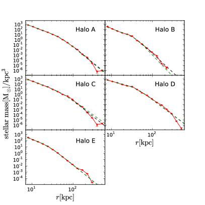
To derive analytical expressions for Eqn. 6 and Eqn. 7, we need an analytical form for the tracer density profile, $\rho(r)$. Fig. 2 shows the radial density profile of stellar mass (red points) in each of the five Aquarius halos. Error bars are obtained from 100 realisations of bootstrap resampling. In most of the cases, these profiles can be described well by a double power law (black dashed lines are double power-law fits that minimise $\chi^{2}$). Significant deviations from a double power law are most obvious in the outskirts of the halos. For example, halo E has a prominent bump at $r\sim 100$ kpc due to a tidal stream.

There are indications that the real MW has a two-component profile, with density falling off more rapidly beyond $\sim 25$ kpc, whereas M31 has a smooth profile out to 100 kpc with no obvious break (e.g. Watkins et al., 2009; Deason et al., 2011; Sesar et al., 2011). Recently, Deason et al. (2014) report evidence for a very steep outer halo profile of the MW. If we believe that MW halo stars originate from the accretion of dwarf satellites, whether the profile is broken or unbroken depends on the details of accretion history (Deason et al., 2013; Lowing et al., 2015). There is an as yet unresolved debate over whether the stellar halo of the MW has an additional contribution from stars formed in situ, in which case a break in the profile may reflect the transition from in situ-dominated regions to accretion dominated regions.

As our mock halo stars (which are all accreted) and observed MW halo stars can be approximated by a double power-law profile, we adopt the following functional form to model tracer density profiles:

$$\rho(r)\propto\left[\left(\frac{r}{r_{0}}\right)^{\alpha}+\left(\frac{r}{r_{0}}\right)^{\gamma}\right]^{-1}.$$ (10)

This equation has three parameters: the inner slope, $\alpha$, the outer slope, $\gamma$, and the transition radius, $r_{0}$.

Previous studies have adopted a single power law to describe the density profile of MW halo stars beyond $r\sim 20$ kpc (e.g. Xue et al., 2008; Gnedin et al., 2010; Deason et al., 2012; Wilkinson & Evans, 1999). Our double power-law form naturally includes this possibility as a special case. We also note that Sakamoto et al. (2003) considered the case of “shadow” tracers with a radial distribution that shares the same functional form with the underlying dark matter. We emphasise that our mock halo stars are not “shadow” tracers; their radial distribution is significantly different from that of the dark matter.

Assuming these analytical expressions for $\Phi(r)$ and $\rho(r)$, Eqn. 6 and Eqn. 7 can be written more explicitly as

$$\begin{split}P(r,v_{r}|\rho_{s},r_{s},\beta,\alpha,\gamma,r_{0})=-\frac{r_{s}^{2\beta-\alpha-\gamma}}{\sqrt{2}\pi r^{2\beta}v_{s}}\int_{R_{\mathrm{inner}}}^{R_{\mathrm{max,t}}}\frac{R^{\prime 2\beta-1}}{\sqrt{\epsilon(r)-\phi(R^{\prime})}}\\ \times\frac{(2\beta-\alpha)(\frac{R^{\prime}}{r_{0}})^{\alpha}r_{s}^{-\gamma}+(2\beta-\gamma)(\frac{R^{\prime}}{r_{0}})^{\gamma}r_{s}^{-\alpha}}{[(\frac{R^{\prime}}{r_{0}})^{\alpha}r_{s}^{-\gamma}+(\frac{R^{\prime}}{r_{0}})^{\gamma}r_{s}^{-\alpha}]^{2}}\mathrm{d}R^{\prime},\end{split}$$ (11)

and

$$\begin{multlined}P(r,v_{r},v_{t}|\rho_{s},r_{s},\beta,\alpha,\gamma,r_{0})=\\ -\frac{r_{s}^{-\alpha-\gamma}l^{-2\beta}}{2^{3/2-\beta}\pi^{3/2}v_{s}^{3}\Gamma(\beta+1/2)\Gamma(1-\beta)}\times\\ \int_{R_{\mathrm{inner}}}^{R_{\mathrm{max,t}}}\mathrm{d}R^{\prime}(\epsilon(r)-\phi(R^{\prime}))^{\beta-1/2}\times\\ \Bigg{\{}\frac{(2\beta+1)R^{\prime 2\beta}\left(\frac{R^{\prime}}{1+R^{\prime}}-\ln(1+R^{\prime})\right)-\left[\frac{1}{(1+R^{\prime})^{2}}-\frac{1}{1+R^{\prime}}\right]R^{\prime 2\beta+1}}{\left[\frac{R^{\prime}}{1+R^{\prime}}-\ln(1+R^{\prime})\right]^{2}}\\ \times\frac{(2\beta-\alpha)\left(\frac{R^{\prime}}{r_{0}}\right)^{\alpha}r_{s}^{-\gamma}+(2\beta-\gamma)\left(\frac{R^{\prime}}{r_{0}}\right)^{\gamma}\,r_{s}^{-\alpha}}{\left[\left(\frac{R^{\prime}}{r_{0}}\right)^{\alpha}\,r_{s}^{-\gamma}+\left(\frac{R^{\prime}}{r_{0}}\right)^{\gamma}\,r_{s}^{-\alpha}\right]^{2}}+\\ \frac{R^{\prime 2\beta+1}}{\left[\frac{R^{\prime}}{1+R^{\prime}}-\ln(1+R^{\prime})\right]\left[\left(\frac{R^{\prime}}{r_{0}}\right)^{\alpha}\,r_{s}^{-\gamma}+\left(\frac{R^{\prime}}{r_{0}}\right)^{\gamma}\,r_{s}^{-\alpha}\right]^{3}}\times\\ \Bigg{[}(2\beta-\alpha)r_{s}^{-\alpha-\gamma}\left(\frac{\alpha}{r_{0}}-\frac{2\gamma}{r_{0}}\right)\left(\frac{R^{\prime}}{r_{0}}\right)^{\alpha+\gamma-1}+\\ (2\beta-\gamma)r_{s}^{-\alpha-\gamma}\left(\frac{\gamma}{r_{0}}-\frac{2\alpha}{r_{0}}\right)\left(\frac{R^{\prime}}{r_{0}}\right)^{\alpha+\gamma-1}-\\ (2\beta-\alpha)r_{s}^{-2\gamma}\frac{\alpha}{r_{0}}\left(\frac{R^{\prime}}{r_{0}}\right)^{2\alpha-1}-(2\beta-\gamma)r_{s}^{-2\alpha}\frac{\gamma}{r_{0}}\left(\frac{R^{\prime}}{r_{0}}\right)^{2\gamma-1}\Bigg{]}\Bigg{\}}.\end{multlined}P(r,v_{r},v_{t}|\rho_{s},r_{s},\beta,\alpha,\gamma,r_{0})=\\ -\frac{r_{s}^{-\alpha-\gamma}l^{-2\beta}}{2^{3/2-\beta}\pi^{3/2}v_{s}^{3}\Gamma(\beta+1/2)\Gamma(1-\beta)}\times\\ \int_{R_{\mathrm{inner}}}^{R_{\mathrm{max,t}}}\mathrm{d}R^{\prime}(\epsilon(r)-\phi(R^{\prime}))^{\beta-1/2}\times\\ \Bigg{\{}\frac{(2\beta+1)R^{\prime 2\beta}\left(\frac{R^{\prime}}{1+R^{\prime}}-\ln(1+R^{\prime})\right)-\left[\frac{1}{(1+R^{\prime})^{2}}-\frac{1}{1+R^{\prime}}\right]R^{\prime 2\beta+1}}{\left[\frac{R^{\prime}}{1+R^{\prime}}-\ln(1+R^{\prime})\right]^{2}}\\ \times\frac{(2\beta-\alpha)\left(\frac{R^{\prime}}{r_{0}}\right)^{\alpha}r_{s}^{-\gamma}+(2\beta-\gamma)\left(\frac{R^{\prime}}{r_{0}}\right)^{\gamma}\,r_{s}^{-\alpha}}{\left[\left(\frac{R^{\prime}}{r_{0}}\right)^{\alpha}\,r_{s}^{-\gamma}+\left(\frac{R^{\prime}}{r_{0}}\right)^{\gamma}\,r_{s}^{-\alpha}\right]^{2}}+\\ \frac{R^{\prime 2\beta+1}}{\left[\frac{R^{\prime}}{1+R^{\prime}}-\ln(1+R^{\prime})\right]\left[\left(\frac{R^{\prime}}{r_{0}}\right)^{\alpha}\,r_{s}^{-\gamma}+\left(\frac{R^{\prime}}{r_{0}}\right)^{\gamma}\,r_{s}^{-\alpha}\right]^{3}}\times\\ \Bigg{[}(2\beta-\alpha)r_{s}^{-\alpha-\gamma}\left(\frac{\alpha}{r_{0}}-\frac{2\gamma}{r_{0}}\right)\left(\frac{R^{\prime}}{r_{0}}\right)^{\alpha+\gamma-1}+\\ (2\beta-\gamma)r_{s}^{-\alpha-\gamma}\left(\frac{\gamma}{r_{0}}-\frac{2\alpha}{r_{0}}\right)\left(\frac{R^{\prime}}{r_{0}}\right)^{\alpha+\gamma-1}-\\ (2\beta-\alpha)r_{s}^{-2\gamma}\frac{\alpha}{r_{0}}\left(\frac{R^{\prime}}{r_{0}}\right)^{2\alpha-1}-(2\beta-\gamma)r_{s}^{-2\alpha}\frac{\gamma}{r_{0}}\left(\frac{R^{\prime}}{r_{0}}\right)^{2\gamma-1}\Bigg{]}\Bigg{\}}.$$ (12)

Here, analogously to Wilkinson & Evans (1999), we have introduced a characteristic velocity, $v_{s}=r_{s}\sqrt{4\pi G\rho_{s}}$. The binding energy, $\epsilon$, angular momentum, $l$, potential, $\phi$, and radius, $R$, have all been scaled by $v_{s}$ and $r_{s}$ and are thus dimensionless, as follows,

$$\epsilon=\frac{E}{v_{s}^{2}},\ l=\frac{L}{r_{s}v_{s}},\ \phi=\frac{\Phi}{v_{s}^{2}},\ R=\frac{r}{r_{s}}.$$ (13)

As mentioned above, $R_{\mathrm{max,t}}$ is the boundary of the tracer distribution and, for most of our analysis, we take $R_{\mathrm{max,t}}=\infty$. Note that Eqn. 11 and Eqn. 12 are deduced by assuming the tracer boundary, $R_{\mathrm{max,t}}$, is smaller or equal to the halo boundary, $R_{\mathrm{max,h}}$. In both Eqn. 11 and Eqn. 12 there are six model parameters.

The phase-space probability of a tracer at radius, $r$, whose radial and tangential velocities are $v_{r}$ and $v_{t}$, can be derived from Eqn. 11 or Eqn 12. The lower limit of the integral is determined by solving

$$\phi(R_{\mathrm{inner}})=\epsilon,$$ (14)

where $\epsilon$ equals $\phi(R)-{v_{r}^{2}}/{(2v_{s}^{2})}$ when only the radial velocity is available, and $\epsilon$ equals $\phi(R)-{v_{r}^{2}}/{(2v_{s}^{2})}-{v_{t}^{2}}/{(2v_{s}^{2})}$ when tangential velocity is also available. The fact that the integral goes from $R_{\mathrm{inner}}$ to $R_{\mathrm{max,t}}$ indicates that the phase-space distribution at radius $r$ has a contribution from tracers currently residing at larger radii, whose radial excursion includes $r$.

3.3 Likelihood and window function

The probability of each observed tracer object, labeled $i$, with radius, $r_{i}$, radial velocity, $v_{ri}$, and tangential velocity, $v_{ti}$, is

$$P_{i}(r_{i},v_{ri},v_{ti}|\rho_{s},r_{s},\beta,\alpha,\gamma,r_{0}).$$ (15)

Dynamical tracers, such as MW globular clusters, BHB stars and satellites, are subject to selection effects. For example, sample completeness is often a function of apparent magnitude (hence distance). If we assume that all selection effects can be described by a window function, then the probability of finding each tracer object, $i$, within the data window is given by the normalised phase-space density

$$F_{i}=\frac{P_{i}}{\int_{\mathrm{window}}P\,\mathrm{d}^{3}r\mathrm{d}^{3}v}.$$ (16)

The integral in the denominator runs over the phase-space window. The likelihood function then has the following form:

$$L=\prod_{i}F_{i}.$$ (17)

It can easily be shown that this likelihood function is equivalent to the extended likelihood function marginalised over the amplitude parameter of the phase-space density (e.g. Barlow, 1990), which we are not interested in. For our mock MW halo star catalogue, we deliberately exclude stars in the innermost region of the halo. These stars have extremely high phase-space density and so make a dominant contribution to the total likelihood, strongly biasing the fit. We find that excluding all stars at $r<7$ kpc removes this bias. The window function in our analysis is then simply $P=0$ at $r<7$ kpc. In real observations, the window function can be much more complicated.

We seek parameters that maximise the value of the likelihood function defined in Eqn. 16 and Eqn. 17. In order to search the high-dimensional parameter space efficiently, we use the software IMINUIT, which is a python interface of the MINUIT function minimiser (James & Roos, 1975).

There are six parameters in Eqn. 11 or Eqn. 12. To make best use of the likelihood method, we treat all six parameters as free. In previous work using this approach the three parameters of the spatial part of the tracer distribution are often fixed to their observed values. We have carried out tests and found that, as expected, three parameter models give results consistent with those using six parameters only when the choice of tracer density profile is close to the true distribution. We recommend that all six parameters should be left free if the observed sample size is large enough to avoid introducing unnecessary bias.

Another source of potential bias in the halo mass estimates of previous studies arises from the use of universal mean mass–concentration relations for dark matter halos. In CDM simulations, the relation between halo mass and concentration has very large scatter (e.g. Neto et al., 2007). Taking halo A as an example, if we use the mass concentration relation from Duffy et al. (2008), the estimated concentration would be around 5.7, which is almost three times smaller than the true value (see Table LABEL:tbl:parameters). This would result in an overestimate of halo mass by almost an order of magnitude, and the corresponding scalelength, $r_{s}$, would be three times larger. The huge scatter in the mass-concentration relation can cause catastrophic problems unless we are fortunate enough that the host halo of the MW does in fact lie on the mean mass-concentration relation.

3.4 Weighting tagged particles

As described in Sec. 2.3, our mock catalogues are created by assigning stars from each single age stellar population to the 1% most bound dark matter particles in their host halo at the time of their formation. The total stellar mass of each population will obviously vary from one population to the next (according to our galaxy formation model), as will the number of dark matter particles actually tagged (according to the number of particles in the corresponding formation halo). The result is that stellar masses associated with individual dark matter particles range over several orders of magnitude. Particles tagged with larger stellar masses correspond to more stars, and thus in principle should carry more weight in the likelihood fit.

To reflect this we could simply reweight each particle according to its associated stellar mass, $M_{*,i}$. However, individual stars are not resolved: the phase-space coordinates of the underlying dark matter particles comprise the maximum amount of dynamical information available from the tagging technique. Therefore, we give each particle a weight $({M_{*,i}}/{\Sigma_{i}{M_{*,i}}})N_{\mathrm{tags}}$. This conserves the total particle number, $N_{\mathrm{tags}}$, but re-distributes this among particles in proportion to the fraction of the total stellar mass they represent. In this way we maintain a meaningful error estimated from the likelihood function.

We also randomly divide stars into subsamples and apply our maximum likelihood analysis to each of these to estimate the effects of Poisson noise. To do so, we assign each weighted particle a new integer weight drawn from a Poisson distribution with mean equal to the weight given by the expression above. We repeat this procedure 10 times, so that we have 10 different subsamples. The expectation values of the total weight for all tagged particles in these subsamples are the same, so this approach can be regarded as analogous to bootstrap resampling. We find this procedure yields consistent error estimates with that obtained from the Hessian matrix of the likelihood surface. From now on, we will only quote errors from the Hessian matrix.

We restrict our analysis to the 10% oldest tagged particles in the main halo. This is to reflect the fact that, in real observations, old halo stars such as blue horizontal branch (BHB) and RR Lyrae stars are most often used as dynamical tracers, because they are approximately standard candles. We also exclude stars bound to surviving subhalos.

3.5 Testing the method

Figure 3: The ratio between input and best-fit halo masses ($x$-axis) versus the ratio between input and best-fit halo concentrations ($y$-axis). Both radial and tangential velocities are used. The red cross is the mean ratio over 750 different realisations, which is very close to 1 on both axes (horizontal and vertical dashed lines). Black solid contours mark the region in parameter plane enclosing 68.3% (1$\sigma$) and and 95.5% (2$\sigma$) of best fit parameters among the 750 realisations.

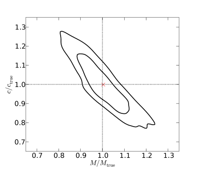
Before fitting the model distribution function to our realistic mock stellar halo catalogues, we test the method with ideal samples of particles that obey Eqn. 12. We applied our maximum likelihood method to 750 sets of 1000 phase-space coordinates ($r$, $v_{r}$ and $v_{t}$) each drawn randomly from the same distribution function of the form given by Eqn. (12). Fig. 3 shows a comparison between the input halo parameters and the recovered best-fit halo parameters. The $x$ axis is the ratio between the best-fit and true-input halo mass, and the $y$ axis the ratio between best-fit and true concentration. The red cross indicates the mean ratios averaged over all the 750 realisations, which is very close to unity (horizontal and vertical dashed lines).

The best-fit halo mass and concentration varies among realisations as a result of statistical fluctuations, as shown in Fig. 3. We note that the shape of these contours indicate a correlation between the recovered halo mass and concentration parameters. The correlation coefficient (i.e., normalised covariance) is -0.89, which implies a strong negative correlation in the model parameter. We will discuss this correlation further in Sec. 5. The above exercise reassures us that our method works with ideal tracers, so we can move on to apply it to the more realistic mock halo stars in our simulations.

4 Results

In this section we investigate how well the true halo mass can be recovered by fitting Eqn. 11 to mock halo stars in cases where: (a) only radial velocities are available (Sec. 4.1) and (b) both radial and tangential velocities are available (Sec. 4.2). In both cases we model the underlying potential with infinite halo boundaries. We refer to parameters estimated with the maximum likelihood technique as best-fit (or measured) parameters, to be compared with the real (or true) parameters taken directly from the simulation.

The total number of tagged particles we used in the five halos is shown in Table LABEL:tbl:num. These are of the order of $10^{5}$, one or two orders of magnitude larger than the tracer samples used by Deason et al. (2012) or Kafle et al. (2012). This permits a robust test of the method free from the effects of sampling fluctuations. Future samples of observed tracers will grow with ongoing and upcoming surveys such Gaia (Prusti, 2012; Gilmore et al., 2012) and other deep spectroscopic surveys like MS-DESI (Eisenstein & DESI Collaboration, 2015) and 4MOST (de Jong et al., 2012).

4.1 Radial velocity only

Figure 4: The best-fit values of $M_{200}$, $c_{200}$ and $\beta$ for the five halos (black dots with errors). Tangential velocities are not used. Error bars are 1$\sigma$ uncertainties obtained from the Hessian matrix and are almost invisible. The 1$\sigma$ errors are comparable to the scatter among the 10 subsamples constructed in Sec. 3.4. For direct comparison we show the true values of $M_{200}$, $c_{200}$ and $\beta$ as red dots.

Table 1: best-fit and true model parameters for each of our five halos. The highlighted rows list the true values of model parameters and the subsequent two rows the corresponding best-fit values when using only radial velocities, $v_{r}$, and using both radial and tangential velocities, $v_{r}+v_{t}$.

	A	B	C	D	E
true $M_{200}[\mathrm{10^{12}M_{\odot}}]$	1.842	0.819	1.774	1.774	1.185
$v_{r}$	1.302 $\pm$ 0.02	1.972 $\pm$ 0.056	1.616 $\pm$ 0.029	1.911 $\pm$ 0.032	0.744 $\pm$ 0.017
$v_{r}+v_{t}$	1.150 $\pm$ 0.003	0.867 $\pm$ 0.013	1.411 $\pm$ 0.013	1.410 $\pm$ 0.005	0.995 $\pm$ 0.014
true $c_{200}$	16.098	8.161	12.337	8.732	8.667
$v_{r}$	8.616 $\pm$ 0.276	3.080 $\pm$ 0.053	7.682 $\pm$ 0.140	6.721 $\pm$ 0.118	8.758 $\pm$ 0.314
$v_{r}+v_{t}$	15.269 $\pm$ 0.097	8.186 $\pm$ 0.107	15.878 $\pm$ 0.199	10.317 $\pm$ 0.039	10.297 $\pm$ 0.144
true $r_{s}[\mathrm{kpc}]$	15.274	23.000	19.685	27.808	24.493
$v_{r}$	25.422 $\pm$ 1.006	81.660 $\pm$ 1.328	30.642 $\pm$ 0.494	37.035 $\pm$ 0.566	20.752 $\pm$ 0.636
$v_{r}+v_{t}$	13.763 $\pm$ 0.088	23.360 $\pm$ 0.328	14.169 $\pm$ 0.183	21.805 $\pm$ 0.086	19.446 $\pm$ 0.287
true $\log_{10}\rho_{s}[\mathrm{M_{\odot}/kpc^{3}}]$	7.193	6.591	7.025	6.646	6.642
$v_{r}$	6.664 $\pm$ 0.034	5.646 $\pm$ 0.016	6.544 $\pm$ 0.019	6.407 $\pm$ 0.018	6.681 $\pm$ 0.038
$v_{r}+v_{t}$	7.278 $\pm$ 0.007	6.610 $\pm$ 0.014	7.321 $\pm$ 0.014	6.857 $\pm$ 0.004	6.852 $\pm$ 0.015
true $R_{200}[\mathrm{kpc}]$	245.88	187.70	242.82	242.85	212.28
$v_{r}$	219.025 $\pm$ 11.155	251.525 $\pm$ 5.962	235.382 $\pm$ 5.786	248.901 $\pm$ 5.786	181.754 $\pm$ 8.579
$v_{r}+v_{t}$	210.144 $\pm$ 1.797	191.234 $\pm$ 3.383	224.984 $\pm$ 3.785	224.962 $\pm$ 1.133	200.241 $\pm$ 3.770
true $\beta$	0.660	0.570	0.587	0.752	0.464
$v_{r}$	0.994 $\pm$ 0.001	1.000 $\pm$ 0.001	1.000 $\pm$ 0.001	0.830 $\pm$ 0.008	0.713 $\pm$ 0.08
$v_{r}+v_{t}$	0.458 $\pm$ 0.002	0.397 $\pm$ 0.002	0.407 $\pm$ 0.002	0.553 $\pm$ 0.001	0.254 $\pm$ 0.003
true $\alpha$	2.926	2.912	3.055	2.007	2.223
$v_{r}$	2.965 $\pm$ 0.490	2.911 $\pm$ 0.007	3.008 $\pm$ 0.011	2.112 $\pm$ 0.009	2.454 $\pm$ 0.023
$v_{r}+v_{t}$	2.774 $\pm$ 0.010	2.770 $\pm$ 0.008	2.962 $\pm$ 0.014	2.012 $\pm$ 0.005	2.413 $\pm$ 0.017
true $\gamma$	6.468	7.485	6.383	6.048	5.256
$v_{r}$	6.650 $\pm$ 0.037	8.362 $\pm$ 0.038	5.884 $\pm$ 0.034	6.031 $\pm$ 0.017	5.297 $\pm$ 0.023
$v_{r}+v_{t}$	6.110 $\pm$ 0.025	8.140 $\pm$ 0.034	5.623 $\pm$ 0.030	5.820 $\pm$ 0.013	5.305 $\pm$ 0.020
true $r_{0}$[$\mathrm{kpc}$]	51.892	38.506	60.040	40.121	24.215
$v_{r}$	53.376 $\pm$ 0.260	38.779 $\pm$ 0.138	57.643 $\pm$ 0.847	42.183 $\pm$ 0.204	26.645 $\pm$ 0.204
$v_{r}+v_{t}$	42.590 $\pm$ 0.345	35.736 $\pm$ 0.111	51.375 $\pm$ 0.935	38.165 $\pm$ 0.100	26.645 $\pm$ 0.294

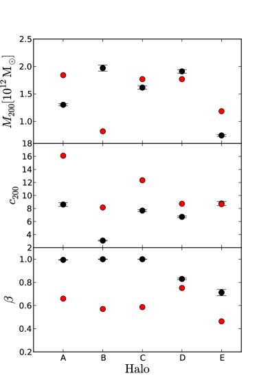
Fig. 4 shows, as black points, the best-fit $M_{200}$, $c_{200}$ and $\beta$ for our five halos in the case where only radial velocities are known. These best-fit parameters are given in Table LABEL:tbl:parameters along with the true halo or tracer properties (shaded in grey), which are plotted as red points in Fig. 4.

Table 2: The total number of tagged particles in each of our five simulated halos.

	A	B	C	D	E
number	181995	225030	184197	365280	120806

Table LABEL:tbl:parameters lists the true and best-fit values of the host halo mass ($M_{200}$), halo concentration ($c_{200}$), scalelength ($r_{s}$), scaledensity ($\rho_{s}$) and virial radius ($R_{200}$). Note only two of these parameters are independent. The best-fit $M_{200}$ values are overestimates of the true values for halos B and D by 140% and 7%, and underestimates for halos A, C and E by 30%, 10% and 35% respectively. Since the number of stars is very large (Table LABEL:tbl:num), the statistical errors are all very small. The systematic biases in the estimates of halo mass and concentration are thus very significant. We find the scatter in parameters among the 10 bootstrap subsamples discussed in Sec. 3.5 is comparable to the statistical error in the fit.

Figure 5: The velocity anisotropy parameter, $\beta$, as a function of radius for stars (blue solid curve) and a randomly selected subsample of dark matter particles (black solid curve) in halo A. Error bars are estimates obtained from bootstrap resampling. Blue and black dashed curves are the mean value of $\beta$ over the whole radial range for stars and dark matter particles.

The measured spatial parameters ($\alpha$, $\gamma$ and $r_{0}$) agree well with the true values obtained from a double power-law fit to the stellar mass density, shown as black dashed lines in Fig. 2. The profiles corresponding to the best-fit parameters are plotted as dashed green lines in the figure. The agreement is especially good on scales smaller than or comparable to the transition radius $r_{0}$. In the outskirts, differences become noticeable for halos B and C. This is due to the fact that there are fewer stars in these regions and the profiles have a significant contribution from coherent streams. As a result, the direct fitting of radial profiles returns parameters that are slightly different from those obtained from the likelihood technique because the latter also involves fitting to the velocity distribution. In addition, the direct fit is dependent on our choice of radial binning.

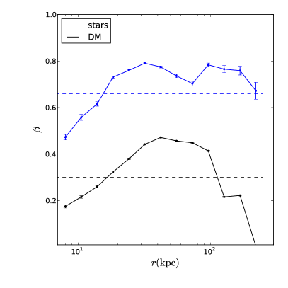
The velocity anisotropy, $\beta$, is poorly estimated. The model assumes $\beta$ to have a single value at all radii. However, the true velocity anisotropy in the simulation does depend on radius: the blue solid curve with errors in Fig. 5 is the velocity anisotropy profile of stars in halo A as a function of distance from the halo centre. We also show the mean value of $\beta$ (0.66 in Table LABEL:tbl:parameters) as the blue dashed line. The poor measurement of $\beta$ is not simply due to radial averaging, because we can see that the estimate of $\beta$ for halo A, 0.994, is significantly greater than the real value over the whole radial range probed. The black curve shows the radial profile of $\beta$ for dark matter particles. There is an obvious offset between the velocity anisotropy profiles of stars (tagged particles) and all dark matter, which we will discuss in detail in Appendix A.

4.2 Radial plus tangential velocity

Figure 6: The measured $M_{200}$, $c_{200}$ and $\beta$. This is similar to Fig. 4 but based on both radial and tangential velocities. Black solid dots with errors show our best-fit model parameters, while red dots show the true values of $M_{200}$, $c_{200}$ and $\beta$.

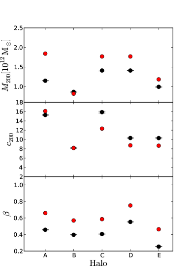
Best-fit parameters when tangential velocities are also included are shown as black points in Fig. 6 and in Table LABEL:tbl:parameters. Compared with the results when only radial velocities are used, we see a reduction in the overall bias of the best-fit parameters with respect to their true values. However, there are still significant discrepancies between best-fit and true parameters, compared with the small errors. $M_{200}$ is underestimated for halos A, C, D and E by 40%, 20%, 20% and 15% respectively. For halo B there is a 5% overestimate. Although the measured host halo masses seem to be worse for halos A, C and D, compared to the case where only radial velocities were used, the agreement between measured and true halo concentrations in the same halos is significantly improved. The best-fit spatial parameters, on the other hand, converge to stable values that agree well with true values.

Compared with Fig. 4, the measurements in Fig. 6 are much more clearly correlated with the true halo properties. In particular, the shape of the best-fit and true $\beta$ curves are in good agreement, although there is approximately a constant offset between them. Tangential velocities are therefore essential for measuring tracer velocity anisotropy, but even with this information there can still be a systematic bias in the absolute value of $\beta$ recovered by distribution function modelling. We return to this point in Appendix A.

4.3 Overall model performance

Figure 7: A phase-space contour plot (kinetic energy, $K$, versus angular momentum, $L$) of mock halo stars (green solid curves) and model predictions (red dashed curves). The left column is based on true halo parameters, true $\beta$ and true spatial parameters of stars. The middle column is identical to the left column, except that $\beta$ has been fixed to its best-fit value in Table LABEL:tbl:parameters (when both radial and tangential velocities are used). Halo and tracer parameters in the right column have all been fixed to be the best-fit parameters with both radial and tangential velocities. Contours for the five halos are presented in different rows, as indicated by texts in the left column of each row.

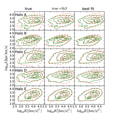
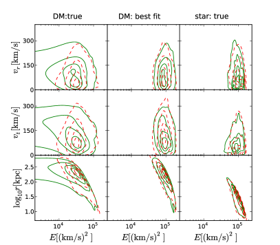
We have shown that the degree of bias between true and best-fit values resulting from our fitting procedure differs from halo to halo. In the current subsection we aim to show how well the model works in recovering the overall phase-space distributions of our mock halo stars. Fig. 7 shows phase-space contour plots for mock halo stars (green solid curves) and compares them with the predictions of our model (red dashed curves). We choose to make the contour plot in terms of two observable quantities: kinetic energy, $K$, and angular momentum, $L$. Each row shows a different halo. In each column, the choice of model parameters is different. In the leftmost column, we use the true values of all parameters. In the case of $\beta$, we take its “true” value to be the velocity anisotropy averaged over the whole radial range. In the central column, we use the true values for all parameters except $\beta$, which is set to be the best-fit value in Table LABEL:tbl:parameters obtained using both radial and tangential velocities. In the rightmost column, we set all parameters to their best-fit values (again using both radial and tangential velocities). Since the green solid curves show data from the simulation, they are identical for all three columns of a given row. The contour levels correspond to the mass density of the 10, 30, 60 and 90% densest cells.

The distribution functions defined by the true parameters (red dashed curves) are a poor description of the mock stars in the left hand column, especially for halos A, C and D where we see a significant over prediction of low angular momentum particles. Halo E is the exceptional case in which we find good agreement. The strongest disagreement in the other halos is, interestingly, mainly due to the biased measurement of $\beta$. In the central column, where we fix the value of $\beta$ to its best-fit value (obtained using both velocity components) we see that the model predictions agree much better with the true phase-space distribution, although some discrepancies remain.

The fact that the model does not properly represent the distribution of mock stars when we use the true value of $\beta$ is indicative of possible deficiencies in the model functional form. We will show in Appendix A that the physical interpretation of $\beta$ in the power-law index, $-2\beta$, of our distribution function as the true velocity anisotropy is not appropriate. Moreover, the approximation of a constant $\beta$ over the whole radial range is problematic, as we know $\beta$ is radially dependent (see Fig. 5). However, this is very likely subdominant because the true value of $\beta$ is above the best-fit value (0.458) over almost the entire radial range (blue solid curve in Fig. 5).

For comparison, the right hand column of Fig. 7 shows that model predictions based on the best-fit parameters give an equally good match to the simulation data. Judging by eye alone, it would be hard to tell whether the middle column shows better or worse agreement than the right hand column. However, judging according to the likelihood ratios, the best-fit halo parameters are indeed a much better description of the data than the true halo parameters ($\gg 3\sigma$). This is also reflected in the small formal errors of the fit.

5 Sources of bias

Fig. 7 indicates that the model is able to recover the general phase-space distribution of the mock halo stars, although there are some subtle factors which significantly bias our best-fit parameter values relative to their true values. There are several possible sources of this bias:

• Correlations among parameters make the model more sensitive to perturbations and, in some cases, a poor fit to one parameter will propagate to affect the others.

• Tracers may violate the assumption of dynamical equilibrium.

• Both the underlying potential and the spatial distribution of tracers may not satisfy the spherical assumption.

• The velocity anisotropy ($\beta$) is not constant with radius as assumed in the model, although this variation is probably subdominant compared with the systematic bias in $\beta$.

• The true dark matter distribution may deviate from the NFW model.

• There are ambiguities in how to model the boundaries of halos.

We have investigated each of these possibilities and found that ambiguity in the treatment of halo boundaries are relatively unimportant; hence we describe their effects in Appendix B. We have investigated the density profiles of the Aquarius halos and found that halo A is not well fit by an NFW profile; instead its inner and outer density profiles are better described by two different NFW profiles of different mass and concentration. This might explain the systematic underestimation of $M_{\mathrm{200}}$. For the other halos, the NFW form is a good approximation and thus deviations from it are not the dominant source of bias.

In Fig. 6 we showed that the velocity anisotropy, $\beta$, varies strongly with radius. The best-fit value of $\beta$ (which is assumed to be constant) turns out to show a significant bias. We will discuss the origin of the bias for $\beta$ in Appendix A. In the following, we will first discuss whether the bias and approximate treatment of $\beta$ affects the fit of the other parameters. In the following subsections, we focus on correlations among model parameters, the spherical assumption and the dynamical state of tracers.

5.1 Correlations among model parameters

Table 3: Correlation matrix of model parameters for halo E

$v_{r}+v_{t}$
	$\beta$	$M_{200}$	$c_{200}$	$\alpha$	$\gamma$	$r_{0}$
$\beta$	1.0	0.025	0.033	-0.00006	-0.007	0.001
$M_{200}$	0.025	1.0	-0.887	-0.207	0.342	0.040
$c_{200}$	0.033	-0.887	1.0	0.252	-0.338	-0.111
$\alpha$	-0.00006	-0.207	0.252	1.0	0.382	0.768
$\gamma$	-0.007	0.342	-0.338	0.068	1.0	0.724
$r_{0}$	0.001	-0.040	-0.111	0.768	0.724	1.0
$v_{r}$ only
	$\beta$	$M_{200}$	$c_{200}$	$\alpha$	$\gamma$	$r_{0}$
$\beta$	1.0	-0.267	-0.787	0.573	0.306	0.507
$M_{200}$	-0.267	1.0	-0.321	-0.244	0.187	-0.073
$c_{200}$	-0.787	-0.321	1.0	-0.384	-0.415	-0.473
$\alpha$	0.573	-0.244	-0.384	1.0	0.574	0.875
$\gamma$	0.306	0.187	-0.415	0.574	1.0	0.799
$r_{0}$	0.507	-0.073	-0.473	0.875	0.799	1.0

Figure 8: The marginalised error contours for all possible combinations of every two out of the six model parameters (halo E). Both radial and tangential velocities are used. Red, blue and purple contours correspond to 1, 2 and 3-$\sigma$ errors. Green dots show the best fit parameters scaled by their true values. The 1-$\sigma$ error ellipses estimated from the covariance matrix are over-plotted in black.

Figure 9: As Fig. 8, but only radial velocities are used.

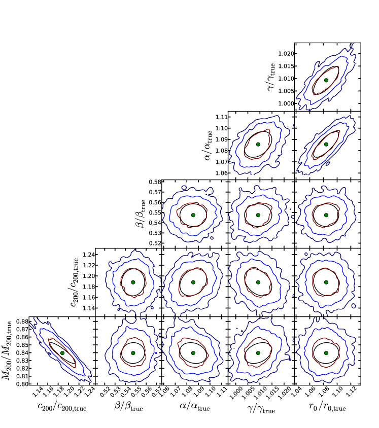
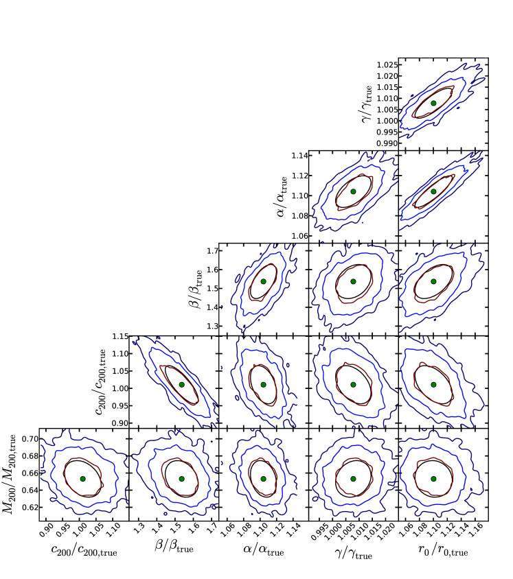
Fig. 3 demonstrated a strong correlation between $M_{200}$ and $c_{200}$. From a modelling perspective, this is dangerous: there are multiple combinations of halo parameters that can give similarly good fits to both the tracer density profile and velocity distribution. In this subsection we ask what causes this correlation and whether there are similar correlations among other parameters. In particular, we have seen that the model gives strongly biased estimates of the velocity anisotropy of stars, $\beta$. We want to check whether this bias propagates to the other parameters.

Fig. 8 shows the marginalised 1, 2 and 3-$\sigma$ error contours for all possible combinations of two model parameters and is for halo E (tangential velocities are included as constraints). Fig. 9 is similar to Fig. 8, but shows the corresponding error contours when only radial velocities are used. All parameters have been scaled by their true values (Table LABEL:tbl:parameters). The error contours are obtained by scanning likelihood values over the full 6-dimensional parameter space. We also overplot as black ellipses the 1-$\sigma$ error from the covariance matrix recovered for halo E. The agreement between the black ellipses and blue error contours is very good in all the panels, indicating the error estimated from the Hessian matrix is robust. The corresponding values of the normalised covariance matrix are also provided in Table LABEL:tbl:cov.

For the other halos, the error contours look qualitatively similar, except for halo A in which the correlation between halo mass and concentration is weaker. This is because the bias in the recovered halo properties of halo A is mostly due to its deviation from an NFW profile. Otherwise, we found the agreement between the error ellipse from the covariance matrix and the scanned error contours are worse for the radial velocity only case of halo A, B and C. This is mainly because the best fit value of $\beta$ touches the upper boundary $\beta=1$ and thus the quadratic approximation is no longer good enough to estimate the error from Hessian matrix, but even in such cases the errors estimated from Hessian matrix is still acceptable with at most a factor of two deviation from the more strictly obtained error contours.

From Fig. 8, Fig. 9 and Table LABEL:tbl:cov, we can see the correlation between $M_{200}$ and $c_{200}$ is very strong when including tangential velocities (covariance close to -1). The correlation is not as strong if only radial velocities are used. To help understand this correlation, we have explored the velocity distribution of tracers predicted by the model using different combinations of $M_{200}$ and $c_{200}$. We verify that, if $M_{200}$ is increased, the predicted velocity distribution of stars extends to larger velocities, with a corresponding reduction in the probability of smaller velocities. A decrease in $c_{200}$ can roughly compensate for this change in the velocity distribution.

It is worth emphasising that although the error contours for $M_{200}$ and $c_{200}$ are highly elongated (corresponding to the correlation between the two), they are still closed, indicating the constraining power is not insignificant. Because these contours represent the statistical error, they can be reduced by increasing the sample size. With our current sample of  $10^{5}$ particles, the statistical errors on $M_{200}$ and $c_{200}$ are controlled to the 1% level, which is negligible compared to the systematic bias in the parameter values. In other words, the true $M_{200}$ and $c_{200}$ values lie well outside the 3$\sigma$ confidence contour, so that statistical fluctuations do not explain the deviation between the fit and the true parameters even after considering the correlation.

It is interesting to see that the best fit $M_{200}$ and $c_{200}$ in Fig. 6 tend to be biased in opposite directions, except for halo A. Such biases are mainly systematic, because the statistical errors are much smaller. This indicates a negative correlation between the systematic biases, similar to the statistical correlation we have seen above. Note that in principle the correlation in the systematic biases could happen along any direction, independent of the statistical correlation, and it is unclear why the two act in the same direction here. A clean and thorough exploration of this involves segregating various model assumptions and adopting a large sample of halos; Han et al. (2015a, b) present part of this work, which will also be discussed in a forthcoming paper by Wang et al. (in preparation). At this stage, we provide some further discussions on this point in our conclusion.

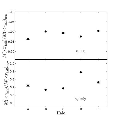
Similar correlation between the velocity anisotropy parameter, $\beta$, and halo properties have been discussed in some previous studies of the Milky Way and dwarf galaxies (e.g. Walker et al., 2009; Wolf et al., 2010; Nesti & Salucci, 2013), though their models are different. In particular, Walker et al. (2009) and Wolf et al. (2010) have reported the mass within the half light radius of dwarf galaxies is relatively insensitive to the value of $\beta$. Here we have also tested whether our model can better constrain the mass within the half-mass radius of our stellar tracers, and the results are shown in Fig. 10.

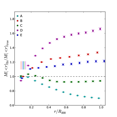
The two panels of Fig. 10 show results based on both radial and tangential velocities (top) and radial velocities only (bottom). Black dots with errors are the ratio between the best fit mass and the true mass within the half mass radius. Encouragingly, we see a very good agreement between the best fit and true mass if tangential velocities are used. The levels of biases are about 3.8%, 0.7% and 2.4% underestimates for halos A, C and D. For halos B and E the mass is overestimated by 0.1% and 0.5% respectively. On the other hand, if only radial velocities are used the bias is much more significant. We underestimate the mass by about 27.8%, 33.2%, 31.4%, 11.1% and 23.8% for the five halos. Compared with Fig. 4, the level of bias becomes significantly smaller for halo B, and is slightly improved for halos A, C and D. Our results suggest if tangential velocities are available, the mass within a fixed radius close to the half-mass radius of tracers are not sensitive to the parameter correlation and can be constrained much better than the total halo mass.

Figure 10: The ratio between the best fit and true mass enclosed within half-mass radius. Errors are obtained through error propagation from the covariance matrix of $\rho_{s}$ and $r_{s}$, with the correlated error between $\rho_{s}$ and $r_{s}$ included.

Figure 11: The best-fit total mass within a fixed radius compared to the true mass within that radius. Both radial and tangential velocities are used. Errors are obtained through error propagation from the covariance matrix of $\rho_{s}$ and $r_{s}$, with the correlated error between $\rho_{s}$ and $r_{s}$ included. The black dashed line marks equality between the measured and true mass.

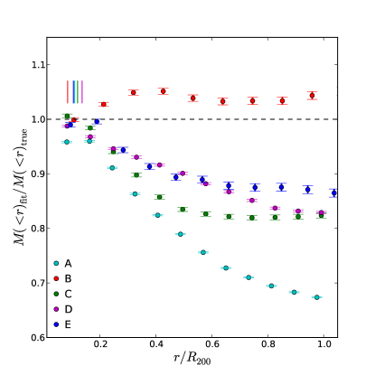
In Fig. 11, we examine the halo mass profiles (cumulative mass within a certain radius as a function of the radius) with the best-fit parameters (when both radial and tangential velocities are included), normalised by profiles with the true parameters. Except for halo B, which gives an acceptable result at all radii, the measurements are very close to the true value for $r\leq 0.2R_{200}$ with a less than 5% bias, though the bias is still significant given the small statistical errors. The measurements become significantly more biased at larger radii. The vertical lines mark the locations of half-mass radii of stellar tracers in the five halos, which are close to $0.1R_{200}$. In practice this means the mass enclosed within 40 to 60 kpc can be more robustly determined as it suffers less from the correlation, and this is usually the radial range for which relatively large numbers of tracers can be observed. Thus the mass measurements reported within 40 to 60 kpc in the literature are expected to be more robust. Note, however, the result here is obtained from stars over the whole radial range. We will further show in Sec. 6 that the mass within about $0.2R_{200}$ can also be determined robustly if stellar tracers are restricted to be within 60 kpc.

In contrast to the strong correlation between $M_{200}$ and $c_{200}$, the correlation between $\beta$ and all the other parameters is very weak if tangential velocities are included. This is fortunate, as it suggests the systematically biased estimate of $\beta$ will not introduce further bias to the other parameters if we have the proper motion information. On the other hand and for the radial velocity only case, the correlation between $\beta$ and the other parameters are actually quite strong, especially in terms of the correlation with halo concentration. This suggests if one only has radial velocity information, it is hard to get a robust estimate of $\beta$ (Fig. 4) and the bias in $\beta$ may affect the fitting of the other model parameters. Compared with the systematic bias in $\beta$, the radial dependence of $\beta$ is actually subdominant.

Correlations between halo parameters ($M_{200}$ or $c_{200}$) and tracer spatial parameters ($\alpha$, $\gamma$ and $r_{0}$) are at the level of a few tens of percent. For the case when tangential velocities are included, an increase in the tracer density outer slope would cause an increase in the recovered halo mass and a corresponding decrease in halo concentration; conversely, an increase in the inner slope would cause a decrease in the halo mass and an increase in the concentration. As a result, uncertainties in the fit to the tracer density profile may further bias the best fit halo parameters. For example, the best-fit (green dashed) curve in the halo C panel of Fig. 2 agrees well with the true profile (red points) inside 170 kpc but is somewhat shallower at larger radii. If we fix the three spatial parameters in our fit to halo C to those given by a conventional reduced-$\chi^{2}$ best-fit to the tracer density (dashed black curve in Fig. 2) the best-fit halo mass is boosted by about 10%. If the tracer density profiles deviate from the double power-law form, these correlations between halo parameters and spatial parameters would introduce further bias to the best-fit halo mass.

Lastly, we note that correlations between the three spatial parameters are strong as well. This quantifies our earlier finding that, in the case of halo A, adding tangential velocities as constraints in the fit makes the outer slope of the tracer density profile shallower and the break radius smaller, but results in very little perceptible change in the overall profile shape. Hence, good fits to the tracer density profiles may not be unique. An increase in $r_{0}$ can be roughly compensated by a corresponding increase of both $\alpha$ and $\gamma$.

5.2 Model uncertainties in the spherical assumption

Figure 12: The host halo masses obtained by fitting to samples of stars drawn from different sky directions and using both radial and tangential velocities. Halos have been rotated based on their dark matter distribution. The $x$-axis and $z$-axis in the rotated system are chosen to be the major and minor principles of the dark matter halo. Measurements are repeated for six survey cones centred at $\pm x$, $\pm y$ and $\pm z$ direction, with opening angle $\pm\frac{\pi}{4}$. Results based on all stars are plotted as the right most point. The red dashed lines show the true values of $M_{200}$.

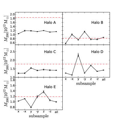
In our analysis and the majority of existing studies of using dynamical tracers to constrain the MW host halo mass, both the tracer population and the underlying potential are modeled assuming spherical symmetry. However, we know dark matter halos in N-body simulations are triaxial (e.g. Jing & Suto, 2002), and the spatial distribution of tracers is unlikely to be perfectly spherical either. It is thus necessary to investigate how the triaxial nature of the underlying dark matter potential and tracer populations affect our results.

To do this, we first rotate the five halos to a new Cartesian coordinate system defined by their principle axes. In this rotated system, the $z$-axis is aligned with the minor axis of the halo and the $x$-axis with major axis of the halo. We then repeat our analysis using six subsamples of tracers drawn from mock ‘survey’ cones pointing along each of the three axes from the origin at the centre of the halo, in the positive and negative directions. The opening angle of each cone is $\pm\frac{\pi}{4}$.

Fig. 12 shows the recovered host halo masses for each of the six cones. Tangential velocities are included in the fit. For a direct comparison, we have also plotted results based on all tracers, as the right most point (from Table LABEL:tbl:parameters). There are significant variations in the results obtained from surveys along different directions, ranging from only a few percent (halo A) to as much as a factor of two (halo D and E). Halos D and E have the most obvious variations. We have explicitly checked that the significant overestimate along the positive $y$-axis of halo D is due to the existence of four relatively massive subhalos ($M_{\mathrm{subhalo}}/M_{\mathrm{200,host}}>1\%$), while the large variation in halo E is due to one prominent stream (see the yellow dots in the bottom panel of Fig. 14 or Fig. 6 in Cooper et al. (2010)), which ranges from $r\sim 80$ kpc ($\sim 0.3R_{\mathrm{200}}$) all the way to the virial radius.

These variations are, however, almost random and uncorrelated with the choice of any particular principle axis, and they change from halo to halo. Halo A has the smallest variation, with all results well below the true host halo mass (red dashed line). Although stronger variations are seen for halo C, all results are again well below the true host halo mass. Thus despite the fact that the variations between directions can be as large as a factor of two, this does not seem to be the dominant cause of the systematic differences between the best-fit and true halo mass in our analysis.

5.3 Unrelaxed dynamical structures

Figure 13: The host halo masses ($M_{200}$) and concentrations ($c_{200}$) measured using a certain fraction of stars that have the earliest infall time and with both radial and tangential velocities. The five columns are for five Aquarius halos, as labeled at the top. The red dashed lines show the true values of $M_{200}$ and $c_{200}$. The top and middle rows are based on the 10% oldest tagged particles. The bottom row is analogous to the top one, except that stars whose parent satellites have not been entirely disrupted yet are excluded.

Figure 14: Phase-space scatter plot (radial velocities versus radial positions) for the 10% oldest tagged particles in the five Aquarius halos. Data points are colour-coded according to their infall time. In sequence, points with yellow, red, magenta, blue and black colours are stars that have earlier and earlier infall times. The bottom right panel is a scatter plot of energy and angular momentum for halo A. Only one out of every 20 points are plotted in order to avoid saturation. Green curves are contours of constant angular momentum and binding energy (see text for details).

Figure 15: Similar to Fig. 12, but only using stars whose parent satellites have been entirely disrupted.

The model distribution function used in our analysis assumes that the tracer population is in dynamical equilibrium and hence the phase-space density of tracers is conserved. Our mock halo stars are all accreted from satellite galaxies, with a range of accretion times. Some prominent phase-space structures, such as stellar streams, may therefore violate the assumption of dynamical equilibrium. In this section we ask how the presence of unrelaxed dynamical structures affects our results.

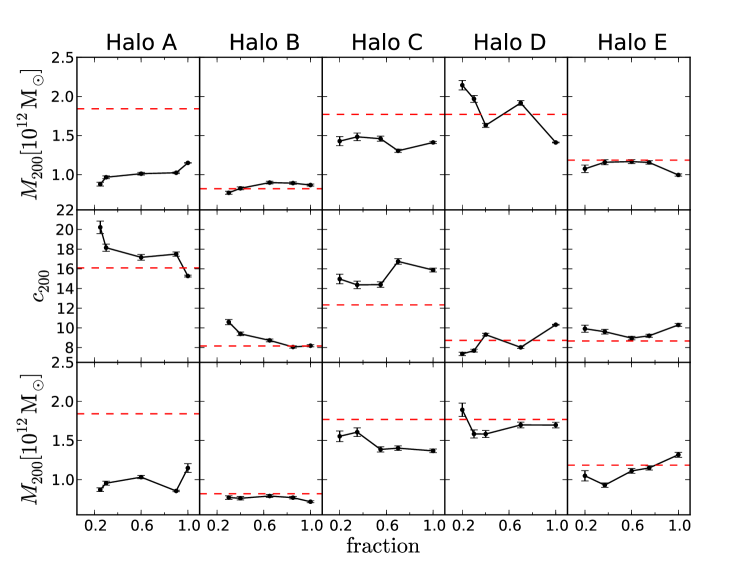
We expect the dynamical state of stars in our mock catalogue to depend on the infall redshift of their parent satellite, at least approximately (satellites on different orbits will have different rates of stellar stripping). We might expect to obtain an improved mass estimate if we use only stars from satellites that fell in earlier, because they have had more time to relax in the host potential. To test this, we rank halo stars according to their infall time. We measure the host halo mass and concentration with samples defined by different cuts in infall time using both radial and tangential velocities, corresponding to roughly the same fraction of stellar mass in each halo. The top and middle rows of Fig. 13 present these parameters as a function of the fraction of stars selected by each cut, for the five different halos. A small fraction corresponds to an earlier mean infall time, but also (obviously) to a smaller sample size. A fraction of $1$ means all the mock stars have been included, hence the corresponding parameters are those listed in Table LABEL:tbl:parameters.

We see fluctuations in the measured halo properties with infall time, but no obvious trends. Using samples of stars with earlier mean infall times does not seem to reduce the bias between best-fit and true parameters. This may be because the dynamical state of tracers depend on many other factors, such as the orbit of their parent satellites. Samples for which the measured halo masses increase produce a corresponding decrease in the measured concentrations, again reflecting the strong correlation between $M_{200}$ and $c_{200}$.

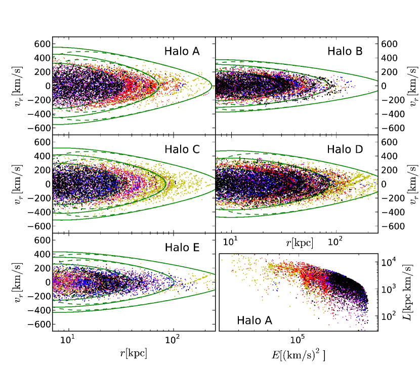
To gain more intuition regarding the dynamical state of halo tracers, Fig. 14 shows phase-space scatter diagrams for mock halo stars (radius, $r$, versus radial velocity, $v_{r}$). Points are colour coded according to the infall time of their parent satellite, with black points corresponding to satellites falling in earliest and blue, magenta, red and yellow points to successively later infall times. Stars with earlier infall times are clearly more centrally concentrated. For points in Fig. 6 with decreasing fraction of stars that fell in earliest, the corresponding particles in Fig. 14 can be found by excluding yellow, red, magenta and blue points by sequence and looking at the remaining points.

Green curves in Fig. 14 are contours of constant angular momentum and binding energy. There are six contours in total, corresponding to three discrete values of binding energy and two discrete values of angular momentum: dashed lines have a higher angular momentum than solid lines. Smaller maximum radius indicates higher binding energy. It is thus straightforward to see that particles with higher binding energy have smaller velocities and are more likely to be found in the inner regions of the halo. Comparing the solid and dashed contours, we see that increasing angular momentum at fixed binding energy causes significant differences in the inner regions of the halo, while at larger radii the two sets of contours almost overlap.

We can see that points with the same colour trace these contours with some scatter, implying that stars whose parent satellites fall in at a particular epoch share similar orbits. This can be seen more clearly in the bottom right panel, which shows a scatter plot of binding energy versus angular momentum for stars in halo A. Points with the same colour occupy regions covering a narrow range of binding energy. The correlation between infall time and binding energy of subhalos has been studied by Rocha et al. (2012). Here we have shown that stars from stripped subhalos show a correlation between infall redshift and binding energy as well.

Although mock stars trace the green contours overall, we can still see some prominent structures. For example, there are two yellow spurs in the outskirts of halo D and one yellow spur in halo E. These correspond to particles that have only just been stripped from their parent satellites. These stars are far from equilibrium: their exclusion causes the rapid change in $M_{200}$ and $c_{200}$ in Fig. 13 between fractions of 1 and $\sim 0.7$ in halos D and E.

To confirm that these unrelaxed phase-space structures can affect our results, we have repeated the above exercise excluding all stars whose parent satellites have not been entirely disrupted. Corresponding results are shown in the bottom row of Fig. 13, again ranking stars by their infall time. Measured halo masses are clearly affected by excluding stars whose parent satellites still survive. For halos A and C, we see some small fluctuations in the measured halo mass, but the systematic underestimate of the true halo mass still remains. The most dramatic changes occur for halos B, D and E. First, the point corresponding to a fraction of 1 for halos D show a significant increase in the recovered mass towards the true values, reinforcing our conclusion that unrelaxed structures are causing significant underestimates of $M_{200}$ in these halos. In fact, most of the yellow dots in halo D panel of Fig. 14 are stars that have been stripped from satellites that still survive. After excluding these, the two highest-fraction points in the halo D panel are based on almost the same sample of stars. We also notice that fluctuations around the true value for the different fractions are reduced in the bottom row (for example, the two lowest fraction points in halo D).

The effects of excluding halo stars from surviving satellites are more ambiguous in halos B and E. The recovered mass of halo B decreases slightly, while for halo E the rightmost point, corresponding to all stars, increases, but the two left most points decrease in amplitude, causing a stronger deviation away from the true values.

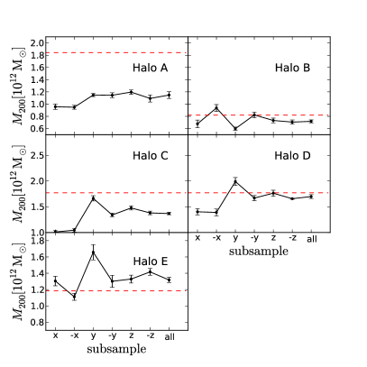
We further investigate how the measurements pointing in different directions change with more relaxed stars. Fig. 15 repeats Fig. 12, using only those stars from satellites that have been entirely disrupted. The measured $M_{200}$ of halo A shows some small variations compared with Fig. 12, but the variation is too small to be significant. The recovered mass of halos B and C improves in some directions, whereas in some other directions it worsens. The most encouraging improvements are for halos D and E. The two measurements along $\pm x$ directions of halo D remain almost unchanged, while the measurements in all the other directions are significantly improved. For halo E the recovered mass increases significantly in all directions.

Our conclusion is thus for halo D (and perhaps E) the underestimates of their host halo masses when all particles are used are mainly due to unrelaxed dynamical structures; for the other halos, the effects of unrelaxed dynamical structures are not obvious. Stars with surviving parent satellites in halos A, B and C could be more dynamically relaxed and thus excluding stars that are expected to be unrelaxed does not make a significant change. Furthermore, we note in a recent work, Bonaca et al. (2014) has developed a new method of determining halo potential using tidal streams. They found individual streams can both under- and overestimate the mass, but the whole stream population is essentially unbiased. Though their method is different from ours, it is possible that a single dynamically hot stream can potentially bias the result, the combination of several streams can help to bring an overall unbiased measurement. A more detailed study quantifying the dynamical state of tracers has been carried out in Han et al. (2015a, b).

6 Model uncertainties in the radial average and implications for real surveys

Figure 16: Best-fit host halo masses using samples of stars in four radial bins, (7-20) kpc, (20-50) kpc, (50-100) kpc and $>$100 kpc. Both radial and tangential velocities are used.

Figure 17: best-fit host halo masses as a function of the outer radius limit of the tracer population ($r<r_{\mathrm{cut}}$). Both radial and tangential velocities are used.

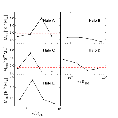
We have seen in the previous section that our maximum likelihood technique recovers different halo mass from sets of tracers with different infall redshifts, or more fundamentally, different binding energies. The sense and magnitude of these differences show no obvious correlations with either quantity, however. Stars falling in earlier typically have high binding energy and are mostly concentrated in the central regions of the halo; since binding energy correlates with radius, we may also expect fluctuations in the recovered halo parameters when using samples of stars drawn from a particular radial range. In this section we investigate this radial dependence. This helps to understand the behaviour of the full model, which averages over all radii. Variations with radius are relevant to observational applications as well, because in practice tracers are often selected from relatively narrow radial ranges, and these ranges may be different for different tracers.

We assign stars to four bins of galactocentric radius: (7-20) kpc, (20-50) kpc, (50-100) kpc and $>$100 kpc. Note in our measurements stars inside 7 kpc have been excluded (Sec. 3.3). The model distribution function is then fit to stars in each bin separately. However, in each case the three spatial parameters of the tracer distribution are fixed to their best-fit values obtained from tracers over the entire radial range, otherwise we would end up with extremely poor extrapolations based on the local density slope. All the other parameters, $M_{200}$, $c_{200}$ and $\beta$, are left as free parameters. The window function, Eqn. 16, is modified appropriately for each bin.

Fig. 16 shows the measured $M_{200}$ as functions of the mean radius of each bin, normalised by the halo virial radius ($R_{200}$). The value of $M_{200}$ varies significantly with the tracer radius. Thanks to the large number of stars (Table LABEL:tbl:num), the errors are all quite small in each bin. For halos A, C and E, stars in the outermost ($r>$100 kpc) and innermost ($r<20$ kpc) bins give underestimates, while stars at 20$<r<$100 kpc give significant overestimates. Similarly, for halos B and D, stars at $r>$100 kpc give underestimates, whereas stars at smaller radii give overestimates.

The velocity anisotropy of tracers, $\beta$, is a function of radius, whereas the model distribution function assumes a single value of $\beta$. To test whether the radial average of $\beta$ may affect our estimates in the host halo mass, we repeated the analysis of Fig. 16 but fixed the value of $\beta$ in each radial bin to either the best-fit value or the true value obtained from the whole population. These measurements are almost identical to the measurements presented in Fig. 16, which confirms our result from Sec. 5.1 that the radial averaging of $\beta$ does not cause further bias in the other parameters.

One feature in Fig. 16 is puzzling at first glance: the best-fit halo masses obtained from the four radial bins individually are all larger than the best-fit halo mass ($M_{200}=1.15$) obtained using stars over the whole radial range. This seems odd, as we might expect that the best-fit $M_{200}$ would be close to the average of the values estimated from the four radial subsamples. The situation is not that straightforward, however, because the likelihood surfaces from the subsamples are superimposed in two dimensional ($M_{200}$ and $c_{200}$) space when the full sample is used. Coupled with the strong correlation between the two parameters, the peak of the final likelihood surface is located around a region where the correlation lines from different subsamples intersect.

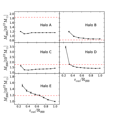
In real observations, there is often a maximum radius of tracers corresponding to the instrumental flux limit. In the present literature this limit is typically much smaller than the expected halo virial radius. Beyond this maximum radius, extrapolations are required to fit the distributions of both the dark matter and tracers. We explore the implications of this directly in Fig. 17 by adopting several outer radial cuts ($r<r_{\mathrm{cut}}$) and reporting the estimated halo mass as a function of the cut radius normalised to the virial radius ($r_{\mathrm{cut}}/R_{\mathrm{200}}$). Unlike Fig. 16, the three spatial parameters are treated as unknown and left free to be constrained by the fit, in order to mimic real observations where the density profiles of tracers is taken directly from the available data.

The overall trends with $r_{\mathrm{cut}}$ in Fig. 17 are very clear: the recovered halo mass is constant at large $r_{\mathrm{cut}}$, and turns up once $r_{\mathrm{cut}}$ becomes small (about 40 per cent of $R_{\mathrm{200}}$). We checked the best-fit values of the tracer spatial parameters in each case, and found they do not vary much with the radial cut as long as $r_{\rm cut}<0.4R_{200}$. This is because the break radius of tracer density profiles in our mock catalogues are smaller than $0.4R_{\mathrm{200}}$ for all the five halos, and so the extrapolation in tracer density is not severe. However, once $r_{\rm cut}$ reduces below $0.4R_{200}$, the outer slope becomes essentially unconstrained. We believe the turn-up behaviour is due to the changing dynamical state of tracers and the extrapolations required to know the underlying potential where there are no tracers.

Previous constraints on the MW halo mass have been derived from tracers roughly covering the range 0.1 to 0.4 $R_{\mathrm{200}}$ ($R_{200}\sim$250 kpc; Deason et al., 2012). Our results suggest that the halo mass, $M_{\mathrm{200}}$, derived from the fitting distribution function of these tracers may be significantly biased even with respect to ‘asymptotic’ results from the same method using all stars in the halo. Furthermore, instead of being a sharp cut, the radial selection functions of real surveys are often complicated, with non-trivial incompleteness as functions of radius and angular position. These selection effects may cause additional bias in the measured host halo mass.

We have shown in Fig. 11 that the total mass within the half-mass radius of the stellar tracer population can be constrained more precisely than the total mass of the halo. We now test if this conclusion is robust to changes in the radial range spanned by the stellar tracers. We repeated the measurements shown in Fig. 11 using only the stars within 60 kpc. The results are displayed in Fig. 18, in the case when both radial and tangential velocities are included in the analysis. The total inferred mass within a fixed radius is strongly biased if this radius is close to the virial radius, $R_{\mathrm{200}}$, but, encouragingly, as the radius is decreased, the measured enclosed mass becomes increasingly close to the true value. Our conclusion that the mass enclosed within the half-mass radius can be constrained reliably still holds even when stellar tracers inside only 60 kpc are considered.

Figure 18: The best-fit total mass within a fixed radius compared to the true mass within that radius, which is obtained from tracers inside 60 kpc and with both radial and tangential velocities. The black dashed line marks equality between the measured and true mass. Vertical lines mark the location of half-mass radii.

7 Conclusions

Several authors have measured parameters of the host halo of our MW, in particular its total mass, by fitting specific forms of the distribution function to the observed distances and velocities of dynamical tracers such as old BHB and RR Lyrae stars, globular clusters and satellite galaxies (Wilkinson & Evans, 1999; Sakamoto et al., 2003; Deason et al., 2012). These models assume that the tracers are in dynamical equilibrium within the host potential. With the help of Jeans theorem, the distribution function of the tracers is further assumed to depend only on two integrals of motion, the binding energy, $E$, and the angular momentum, $L$. In the case of a separable function of $E$ and $L$, the distribution function can be obtained through Eddington inversion of the tracer density profile.

In this paper we have extended earlier analytical forms of the MW halo distribution function to the case of the NFW potential, which is of most relevance to CDM-based models. We generalised the radial distribution of tracers (halo stars) to a double power law, which is suggested by recent observational results and simulations. We used a maximum likelihood approach to fit this model distribution function to a realistic mock stellar halo catalogue of distances and radial velocities, constructed from the high resolution Aquarius $N$-body simulations using the particle tagging technique of Cooper et al. (2010). Our aim was to test the model performance and assumptions. We considered cases with and without additional tangential velocity data. Our conclusions are as follows:

• The best-fit host halo virial masses and concentrations are biased from the true values, with the level of bias varying from halo to halo.

• Adding tangential velocity data substantially reduces this bias, but does not eliminate it. For example, for halo B the agreement between measured and true halo mass is very good (a 5% overestimate) if tangential velocities are used, but for halo A, a 40% underestimate persists even with this additional constraint. The inclusion of tangential velocities therefore is crucial for accurate measurements of both host halo and tracer properties, especially for the velocity anisotropies of the tracers.

• A strong negative correlation between the host halo mass and the halo concentration is found in our analysis.

• The model gives a strongly biased measurement of the velocity anisotropies of stars.

• If tangential velocities are available, the correlation between $\beta$ and all the other parameters are very weak. If only radial velocities are used, $\beta$ is strongly correlated with other parameters and the bias in $\beta$ will be propagated to these parameters. This is because when tangential velocities are not available, we have to rely on the model functional form to infer the unknown tangential component and hence $\beta$.

• Various sources contribute to the biased estimates of halo properties. Violation of the spherical assumption is relatively sub-dominant for the five Aquarius haloes. Violation of the dynamical equilibrium assumption, caused for example by streams, could affect the fits significantly, although we do not observe a systematic sign for the bias in $M_{200}$ (that is, unrelaxed substructures cause underestimates in some cases and overestimates in others).

• When including tangential velocities, the systematic bias tends to happen along the correlation direction of $M_{200}$ and $c_{200}$ except for halo A.

• In contrast to the significantly biased measurements of $M_{200}$ or $c_{200}$, the model gives good constraints on the total mass within the half-mass radius of stellar tracers when including tangential velocities.

The strong correlation between $M_{200}$ and $c_{200}$ arises because changes in the corresponding tracer velocity distribution due to the increase of one of these parameters can be roughly compensated by the other. The correlation between $M_{200}$ and $c_{200}$ is not as strong for the radial velocity only case, which is probably overwhelmed by the strong correlation between $\beta$ and the other parameters, reflecting the fact that the dominant source of bias is the model dependent fit of the tangential component. If the model fails to properly reflect the true phase-space distribution of tracer objects, the best fit $\beta$ and other parameters will be strongly biased.

There are different combinations of halo parameters which give similar likelihood values along the correlation direction. Thus the model is vulnerable to perturbations (for example from dynamically hot structures). This can be seen from Fig. 6: the best fit $M_{200}$ and $c_{200}$ are offset in opposite directions with respect to their true parameter values. This is not the case for halo A, because the dominant source of bias for halo A is the deviation from the NFW model, and the error contour of $M_{200}$ and $c_{200}$ is not as elongated as the other halos. More detailed discussions about this halo will be given in a future study (Han et al., 2015b).

It is, however, confusing to see that although the systematic bias tends to happen along the correlation direction of $M_{200}$ and $c_{200}$, it is much larger than the statistical errors. For example, we can see clearly in Fig 8 that the best fit $M_{200}$ is about 15$\sigma$ away from its true value. This is probably because the statistical error in our analysis does not account for the correlations introduced by phase-space structures or clumps. Our mock stellar halo catalogue contains a very large number of stars. However, these individual stars are not completely independent of each other. Structures such as coherent streams are highly correlated in phase space and it is possible the true number of independent components is much smaller than the total number of stars. To quantify the true number of degrees of freedom by considering correlated phase structures is beyond the scope of our current study. A more detailed discussion is given by Han et al. (2015a, b), in which we introduce a new method based on the steady state assumption, independent of any other assumptions about the model functional form.

Encouragingly, we found the mass within the half-mass radius of the tracer population to be relatively insensitive to the parameter correlations and can be constrained more robustly once tangential velocities are used. This is true even when only stars within about 60 kpc are available. Similar correlations between model parameters and the robustness of the best constrained mass within a fixed radius have been reported and discussed in previous work (e.g. Deg & Widrow, 2014; Kafle et al., 2014; Wolf et al., 2010), although these models are quite different from ours. For our model, the correlation could be closely related to the fact that there are relatively few stars outside $0.2R_{\mathrm{200}}$, beyond which the stellar radial profiles drop very quickly. Given the large number of dynamical tracers inside $0.2R_{\mathrm{200}}$, it is not surprising to find that the mass within this radius can be better constrained. In contrast, the total halo mass, $M_{\mathrm{200}}$, is dominated by mass in the outskirts of the halo and more tracers at large radii are required to have better constraints.

Further information needs to be incorporated into the model to weaken the correlation between mass and concentration. For example, including more tracers at large radii (perhaps from tidal streams) may help to weaken the correlation and improve the measurements of mass in the outer halo. Satellite galaxies and globular clusters in the outer parts of the halo with proper motion measurements could be useful. Having two populations of tracers at two different radial ranges could also be very helpful (e.g. Walker & Peñarrubia, 2011). This would enable us to constrain the mass at two different half-mass radii and hence the entire mass profile can be fixed. More detailed investigations regarding the nature of correlation between $M_{200}$ and $c_{200}$ have been carried out by Han et al. (2015a, b).

The correlations between velocity anisotropy, $\beta$, and all other parameters are very weak when including tangential velocities. This is fortunate, because we know that the model can give systematically biased estimates of $\beta$ for stars; this particular bias is not propagated to the other parameters when including tangential velocities. However, if only radial velocities are available, the condition becomes very different. The correlation between $\beta$ and all the other parameters is strong. Combined with the biased measurements of $\beta$ in Fig. 4, this suggests that if proper motions are not available, it will be difficult to obtain robust constraints on $\beta$ and the bias may affect the fitting of the other parameters. Only by including tangential velocities can the correlation between $\beta$ and the other parameters be broken and $\beta$ be better constrained.

In addition to the correlation between halo mass and concentration, relatively weak but still significant correlations exist between these halo parameters and the three parameters describing the spatial variation of tracer density. When including tangential velocities, we found that a steeper inner slope gives a lower estimate of halo mass, while a steeper outer slope gives an higher estimate. If the true tracer density profile deviates from the double power-law form, the resulting bias will be propagated to the best-fit values of the halo parameters.

The model distribution function requires tracers to be in dynamical equilibrium, with time-independent phase-space density. In reality, stars stripped from satellite galaxies can have highly correlated orbits that violate this assumption. We were able to test how well the assumption holds for our mock halo stars. Perhaps surprisingly, we do not find any systematic correlation of the recovered halo mass with the infall redshift of tracer subsamples. This suggests that the dynamical state of halo tracers depends on other factors, such as their orbits, and not only their infall time. Dynamical relaxation is nevertheless a factor: excluding stars stripped from surviving satellites improves the agreement between best-fit and true halo masses in two cases (halos D and E). This cut eliminates dynamically hot structures that can be identified by eye in these halos.

Beyond all these assumptions and uncertainties in the model itself, in real observations the maximum observable radius of dynamical tracers may be much smaller than the halo virial radius. We found tracer subsamples selected over different ranges of radius can give significantly different estimates of the host halo mass, even if the three parameters describing the density of tracers are fixed to be those derived from the whole tracer population. An outer radius limit results in biased measurements of $M_{200}$ if it significantly smaller than the virial radius. For example, the recovered halo masses of halos A, B, C and D converge for outer radius limits larger than $r\sim 0.4R_{\mathrm{200}}$ but give systematically larger masses for smaller radial limits. For one halo, E, this overestimation occurs for limits $r\lesssim 0.8R_{\mathrm{200}}$. There are two reasons behind this radial dependence: stars at different radii have significantly different dynamical state and extrapolations to larger and smaller radii become less accurate when only a limited radial range is sampled.

Real surveys have complex selection functions for stars, which depend on both radial distance and angular position. Particular classes of tracers may be very sparsely sampled. The observed parallax, radial and tangential velocities of halo stars include observational uncertainties which depend strongly on distance. Although a large sample of tracers with exact coordinate and velocity information from our mock stellar halo catalogue have enabled us to investigate the model performance, it will be important to consider realistic observational errors and sample selection effects in future studies aimed at forecasting the performance of real surveys.

We conclude that methods to estimate the mass of the Milky Way halo using the kind of distribution functions we have investigated here need to be used with extreme caution. This is particularly true when estimating the total virial mass. Restricting the estimate to the mass interior to $r\sim 0.2R_{\mathrm{200}}$ is considerably more reliable. In any case, mock catalogues like those we have analysed here and made publicly available in Lowing et al. (2015) are required to assess the reliability of any particular mass estimation method.

Appendix A Origin of the bias in $\beta$

Figure 19: phase-space distributions of mock stars in halo A (left) and of dark matter in the same halo (right). The top panels in either plots show 2D distributions in the plane of binding energy, $E$, and angular momentum, $L$. $E$ and $L$ have been scaled to be dimensionless. The middle and bottom panels show 1D angular momentum distributions of stars (likewise DM) at two fixed values of $E$, indicated by the horizontal black dashed curves in the top panels. Red and green dashed lines are power-law distributions with arbitrary normalizations, predicted from the velocity anisotropy of all stars (or DM) and stars (or DM) in each binding energy range.

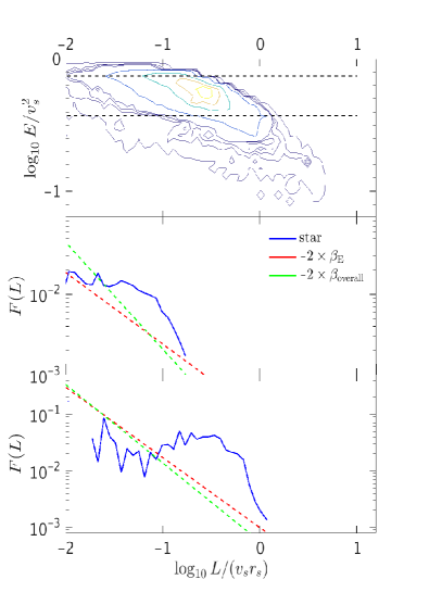
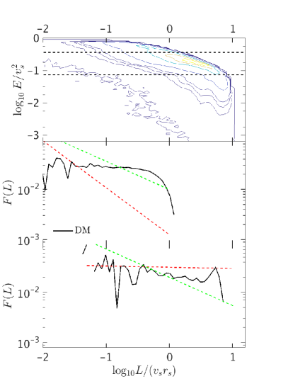
A.1 Origin of the bias

In Fig. 6 we showed that there is a systematic bias between the best-fit and true value of $\beta$. We now show in the left panels of Fig. 19 the phase-space distribution of stars in halo A (top panel, binding energy, $E$, versus angular momentum, $L$) and the one dimensional angular momentum distribution at two fixed values of $E$ (the second and third panels from the top, respectively) indicated by the horizontal dashed lines in the top panel. $E$ and $L$ have been normalised so that they are dimensionless (see Eqn. 13). We only show results based on halo A; for the other halos our conclusions are the same.

In the top panel we see that, for a fixed value of $E$, there is an upper limit to $L$ which increases with decreasing $E$. This is the maximum allowed value of angular momentum, corresponding to circular orbits with zero radial velocity at fixed $E$. In the next two panels, we show the angular momentum distributions at different values of $E$ have similar features. They are both flat at small values of $L$ and drop quickly when $L$ approaches its upper limit. For comparison, we also plot two lines of the form $F(E,L)\propto L^{-2\beta}$, where $\beta$ is the velocity anisotropy obtained from stars in the energy slice, $\beta_{\mathrm{E}}$ (red dashed lines), or the full sample, $\beta_{\mathrm{overall}}$ (green dashed lines). $\beta_{\mathrm{overall}}$ is the same in both panels and is simply the true value of $\beta$ from Table LABEL:tbl:parameters (0.66). The values of $\beta_{\mathrm{E}}$ are 0.442 and 0.618 for the middle and bottom panels respectively. Neither of the two could give a satisfactory description of the true distribution (blue curve). This implies that the physical interpretation of the power-law index in our distribution function as $-2\beta$ is inaccurate, and this is the origin for the systematic bias of $\beta$. The true distribution function must be more complex.

We also notice that the best-fit value of $\beta$ for halo A is $0.458$ (Table LABEL:tbl:parameters), which predicts a power-law slope shallower than the green dashed lines and is also shallower than the red dashed line in the bottom panel, but it is still a poor match to the distributions (blue curve) in Fig. 19. If we fix the power-law slope in the model according to the true anisotropy of the full sample, this results in better agreement with tangential velocity distribution but a much poorer agreement with the radial velocity distribution. Afterall, our maximum likelihood approach is designed to fit the velocity and spatial distributions of stars, not the distributions of binding energy or angular momentum.

A.2 Why stars are more radially biased than dark matter?

The $\beta$ profile of dark matter particles have been studied in earlier works. For example, Wojtak et al. (2008); Wojtak et al. (2009) looked at the distribution functions of dark matter particles in halos of mass $10^{14}$ to $10^{15}M_{\odot}$. Although the details of their modelling and the mass range of halos are different from ours, their model distribution function can recover well the true $\beta$ of dark matter particles in their simulation. We therefore examine the angular momentum distribution of dark matter particles in our simulations in the three right panels of Fig. 19.

In the top panel, we see dark matter particles can extend to much lower binding energy than stars. Black curves in the middle and bottom panels show the angular momentum distribution at two fixed values of $E$. We again plot two lines of the form $F(E,L)\propto L^{-2\beta}$. Red and green lines are predicted from the velocity anisotropy of dark matter particles in the energy slice or from the the full sample respectively. At $E\sim 10^{-0.4}v_{s}^{2}$, the agreement between the red dashed lines and the shape of the $L$ distributions is quite poor, whereas at a lower binding energy ($E\sim 10^{-1.1}v_{s}^{2}$), we see a better agreement. We have looked at many different choices of $E$ in this regard, and found that for less bound dark matter particles, their velocity anisotropy correctly predicts the power-law slope of their $L$ distribution. This means the model distribution function describes better systems of less bound dark matter particles. However, for dark matter particles that are more tightly bound, the velocity anisotropy is not as well correlated with the power-law slope of the $L$ distribution. This is the same as the stellar case, although the discrepancy for dark matter particles is smaller.

Stars in the stellar halo are clearly a biased population of tracers with respect to dark matter particles in the simulation. Their orbits are more radial (Fig. 5) corresponding to a higher $\beta$. However, the difference in $\beta$ is not only because stars are more dynamically bound than dark matter particles: we have explicitly checked that, for a given fraction of the most bound dark matter particles, orbits are still more tangentially biased than stars with the same range of binding energy. The fact that stars are more radially biased than dark matter particles thus has more fundamental physical origin. First of all, in our model halo stars are all accreted from subhalos, while dark matter particles are added to the main halo by both clumpy and smooth accretion. We have calculated the velocity anisotropy of dark matter accreted from subhalos only, and found these particles are more radially biased than all the dark matter particles as a whole. This is probably because the clumps in which these particles are accreted (i.e. subhalos) have more radially biased orbits. Furthermore, halo stars in our analysis are tags placed on the most bound dark matter particles in progenitor subhalos, which have then been stripped and mixed into the main halo. Lowing et al. (2015) have found the halo stars are dominated by contributions from a few massive satellites. As the most bound parts of these satellites have been stripped into the halo, the satellites are more likely to have been on highly radial orbits, imparting a radial bias to halo stars. In contrast, dark matter particles enter the main halos in our simulations through quite different mechanisms, with both clumpy and smooth accretion (Wang et al., 2011).

Appendix B Uncertainties in modelling the halo boundaries

For all the analysis in the main text, we have been assuming the spatial extent of both NFW halos and tracers are infinite ($r_{\mathrm{max,h}}=\infty$ and $r_{\mathrm{max,t}}=\infty$). It is, however, necessary to investigate whether the different choices of halo and tracer boundaries could affect our measured halo properties.

As we have mentioned in Sec. 3.2, in principle tracer boundaries ($r_{\mathrm{max,t}}$) can be different from halo boundaries. Here for simplicity we assume $r_{\mathrm{max,h}}=r_{\mathrm{max,t}}$. We tried four different choices of halo boundaries ($r_{\mathrm{max,h}}$), ranging from twice to five times the halo virial radius. We avoid using boundaries at exactly the halo virial radius because our mock halo stars can extend beyond $R_{200}$, while the mass distribution in the FoF group distribute continuously and extend further than $R_{200}$. A sharp cut at $R_{200}$ is thus not realistic.

The best-fit host halo masses and concentrations as functions of halo boundaries are presented in Fig. 20. The velocity anisotropy $\beta$ almost does not change with the different choices of halo boundaries, and thus we do not show them. Dashed red lines are true values of halo masses and concentrations.

The measured halo masses increase with the decrease in halo boundaries, and the halo concentrations decrease accordingly, reflecting again the strong correlation between the two parameters. The choice of halo boundary that gives the best match between measured and true halo mass varies from halo to halo. For halo B, the best fit halo masses and concentrations almost do not change with the choice of halo boundaries when $r_{\mathrm{max,h}}\geq 3R_{\mathrm{200}}$ and agree well with the true values. At $r_{\mathrm{max,h}}=2R_{\mathrm{200}}$, the measured host halo mass gets significantly larger, indicating for halo B finite halo boundaries do not help to improve the fitting. For halo C, $r_{\mathrm{max,h}}=2R_{\mathrm{200}}$ gives a very good match between the best-fit and true halo mass and concentration, demonstrating a finite halo boundary works better than infinite boundaries at least for halo C.

The estimated halo mass of halo A is closest to the true value when halo boundary is chosen at twice the virial radius. However, the estimated halo concentration at that boundary deviates significantly from the true concentration, suggesting the discrepancy between best-fit and true host halo mass of halo A could not be dominated by how boundaries are modeled. For halo D and E, we know already because of the existence of unrelaxed dynamical structures, the host halo masses are significantly underestimated, and thus the best match between measured and true halo parameters at twice (halo E) and four times (halo D) the virial radius demonstrates the entangling of different model uncertainties, which canceled with each other to give a good prediction.

Figure 20: The measured host halo mass (top row) and concentration (bottom row) as functions of the halo boundaries in the model.

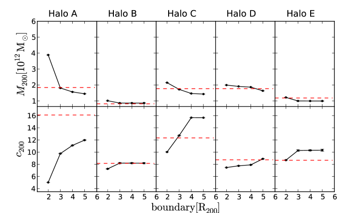
Appendix C Dark matter particles as tracers

Table 4: best-fit parameters from the phase-space distribution of dark matter particles

	A	B	C	D	E
$M_{200}[\mathrm{10^{12}M_{\odot}}]$	2.811 $\pm$ 0.024	1.227 $\pm$ 0.012	2.868 $\pm$ 0.024	2.727 $\pm$ 0.029	1.776 $\pm$ 0.015
$c_{200}$	4.458 $\pm$ 0.098	4.845 $\pm$ 0.105	6.031 $\pm$ 0.106	3.903 $\pm$ 0.104	5.296 $\pm$ 0.108
$r_{s}[\mathrm{kpc}]$	63.499 $\pm$ 1.116	44.315 $\pm$ 0.773	47.257 $\pm$ 0.683	71.799 $\pm$ 1.516	45.867 $\pm$ 0.757
$\log_{10}\rho_{s}[\mathrm{M_{\odot}/kpc^{3}}]$	5.997 $\pm$ 0.021	6.078 $\pm$ 0.021	6.297 $\pm$ 0.018	5.868 $\pm$ 0.025	6.166 $\pm$ 0.020
$R_{200}[\mathrm{kpc}]$	283.078 $\pm$ 7.965	214.715 $\pm$ 5.956	285.003 $\pm$ 6.482	280.225 $\pm$ 9.529	242.901 $\pm$ 6.357
$\beta$	0.266 $\pm$ 0.004	0.159 $\pm$ 0.005	0.259 $\pm$ 0.005	0.217 $\pm$ 0.006	0.090 $\pm$ 0.005

In Sec. A we show the velocity anisotropies of dark matter particles agree better with the distribution function model than those of stars. Furthermore, dark matter particles are more radially extended than stars and might probe better the underlying potential in outskirts. Thus we ask whether better constraints on the halo properties can be achieved by using dark matter particles as tracers. Obviously, it is not possible to directly observe the dynamics of dark matter, but asking this question helps to deepen our understanding of the model. The answer is, unfortunately, no. By using dark matter particles as tracers we end up with significant overestimates of the host halo mass, at least for our five Milky Way analog halos. These measurements are shown in Table LABEL:tbl:DM, where we have used a randomly selected subsample of all dark matter particles in the halo FoF group (one particle out of every 5,000 in the simulation). We have explicitly checked that this conclusion does not change if we randomly select different subsamples of dark matter, remove dark matter particles in substructures or restrict them to be inside the halo virial radius. Both radial and tangential velocities have been used in this analysis.

To explore the reasons behind this, we present in Fig. 21 phase-space contour plots for dark matter particles and stars in the simulation and compare these with realizations drawn directly from the model distribution function. We only show plots based on halo A; for the other halos the conclusion is the same. Distributions of binding energy versus radial velocity, $v_{r}$, tangential velocity, $v_{t}$, and radius, $r$, have been plotted separately, so that we are able to see how well the model prediction agrees with the true distribution of $v_{r}$, $v_{t}$ and $r$ for dark matter particles in the simulation.

It is very clear to see that, with true halo parameters, the model predictions deviate significantly from the empirical distribution of $r$, $v_{r}$ and $v_{t}$ at low binding energy (left column). On the other hand, the best fit model agrees much better with the data (middle column). This improved agreement is caused by an overestimate of the host halo mass, leading to a deeper potential and increased binding energy for tracer particles. As a result, the sample becomes more dynamically bound and agrees better with the model.

Our conclusion is therefore that, although the model distribution function gives a better approximation in the velocity anisotropy of dark matter particles, the predicated phase-space distribution at the low binding energy end is very poor. By construction, the distribution function only describes closed systems. This not only requires that the tracer population should be bound and truncated, but also results in a sharp cut-off in binding energy that is a poor description of particle distribution in the low energy end. Compared with all dark matter particles, the star particles in our simulation are more dynamically bound and centrally concentrated (see the right column) and are thus not sensitive to the low binding energy tail of the dark matter distribution. Using stars rather than dark matter particles therefore insulates the fit from deficiencies of the distribution function model at the low binding energy tail.

Figure 21: The phase-space density of dark matter particles or stars in halo A (green solid) and model predictions (red dashed). The contours mark the 10th, 30th, 60th and 90th percentiles of the 2D density distribution in parameter plane. We present contour plots of binding energy, $E$, versus radius, $r$, radial velocity, $v_{r}$, and tangential velocity, $v_{t}$. For simplicity we only use the magnitudes of $v_{r}$ and $v_{t}$, so all quantities are positive. In deducing the binding energy, we use the analytical NFW potential model. Green contours in the left and middle columns are based on dark matter particles in the simulation, while in the right column we plot contours for stars. For the left, middle and right columns, true halo parameters, dynamical best-fit halo parameters from dark matter particles and true halo parameters are adopted in the potential model respectively. The lines are iso-density contours that contain the 10,30,60 and 90% densest cells.

References

- An et al. (2012) An J., Evans N. W., Deason A. J., 2012, MNRAS, 420, 2562
- Barber et al. (2014) Barber C., Starkenburg E., Navarro J. F., McConnachie A. W., Fattahi A., 2014, MNRAS, 437, 959
- Barlow (1990) Barlow R., 1990, Nuclear Instruments and Methods in Physics Research A, 297, 496
- Bartelmann & Schneider (2001) Bartelmann M., Schneider P., 2001, PhysRep, 340, 291
- Battaglia et al. (2005) Battaglia G., Helmi A., Morrison H., Harding P., Olszewski E. W., Mateo M., Freeman K. C., Norris J., Shectman S. A., 2005, MNRAS, 364, 433
- Bell et al. (2010) Bell E. F., Xue X. X., Rix H.-W., Ruhland C., Hogg D. W., 2010, AJ, 140, 1850
- Bell et al. (2008) Bell E. F., Zucker D. B., Belokurov V., Sharma S., Johnston K. V., Bullock J. S., Hogg D. W., Jahnke K., de Jong J. T. A., Beers T. C., Evans N. W., Grebel E. K., Ivezić Ž., Koposov S. E., Rix H.-W., Schneider D. P., Steinmetz M., Zolotov A., 2008, ApJ, 680, 295
- Bonaca et al. (2014) Bonaca A., Geha M., Küpper A. H. W., Diemand J., Johnston K. V., Hogg D. W., 2014, ApJ, 795, 94
- Bower et al. (2006) Bower R. G., Benson A. J., Malbon R., Helly J. C., Frenk C. S., Baugh C. M., Cole S., Lacey C. G., 2006, MNRAS, 370, 645
- Boylan-Kolchin et al. (2011) Boylan-Kolchin M., Bullock J. S., Kaplinghat M., 2011, MNRAS, 415, L40
- Boylan-Kolchin et al. (2012) Boylan-Kolchin M., Bullock J. S., Kaplinghat M., 2012, MNRAS, 422, 1203
- Boylan-Kolchin et al. (2013) Boylan-Kolchin M., Bullock J. S., Sohn S. T., Besla G., van der Marel R. P., 2013, ApJ, 768, 140
- Busha et al. (2011) Busha M. T., Marshall P. J., Wechsler R. H., Klypin A., Primack J., 2011, ApJ, 743, 40
- Carollo et al. (2010) Carollo D., Beers T. C., Chiba M., Norris J. E., Freeman K. C., Lee Y. S., Ivezić Ž., Rockosi C. M., Yanny B., 2010, ApJ, 712, 692
- Carollo et al. (2007) Carollo D., Beers T. C., Lee Y. S., Chiba M., Norris J. E., Wilhelm R., Sivarani T., Marsteller B., Munn J. A., Bailer-Jones C. A. L., Fiorentin P. R., York D. G., 2007, Nature, 450, 1020
- Cautun et al. (2014) Cautun M., Frenk C. S., van de Weygaert R., Hellwing W. A., Jones B. J. T., 2014, MNRAS, 445, 2049
- Cautun et al. (2014) Cautun M., Hellwing W. A., van de Weygaert R., Frenk C. S., Jones B. J. T., Sawala T., 2014, MNRAS, 445, 1820
- Cooper et al. (2010) Cooper A. P., Cole S., Frenk C. S., White S. D. M., Helly J., Benson A. J., De Lucia G., Helmi A., Jenkins A., Navarro J. F., Springel V., Wang J., 2010, MNRAS, 406, 744
- Cooper et al. (2013) Cooper A. P., D’Souza R., Kauffmann G., Wang J., Boylan-Kolchin M., Guo Q., Frenk C. S., White S. D. M., 2013, MNRAS, 434, 3348
- Cuddeford (1991) Cuddeford P., 1991, MNRAS, 253, 414
- de Jong et al. (2012) de Jong R. S., Bellido-Tirado O., Chiappini C., Depagne É., Haynes R., Johl D., Schnurr O., Schwope 2012, in Society of Photo-Optical Instrumentation Engineers (SPIE) Conference Series Vol. 8446 of Society of Photo-Optical Instrumentation Engineers (SPIE) Conference Series, 4MOST: 4-metre multi-object spectroscopic telescope. p. 0
- Deason et al. (2011) Deason A. J., Belokurov V., Evans N. W., 2011, MNRAS, 416, 2903
- Deason et al. (2012) Deason A. J., Belokurov V., Evans N. W., An J., 2012, MNRAS, 424, L44
- Deason et al. (2013) Deason A. J., Belokurov V., Evans N. W., Johnston K. V., 2013, ApJ, 763, 113
- Deason et al. (2012) Deason A. J., Belokurov V., Evans N. W., Koposov S. E., Cooke R. J., Peñarrubia J., Laporte C. F. P., Fellhauer M., Walker M. G., Olszewski E. W., 2012, MNRAS, 425, 2840
- Deason et al. (2014) Deason A. J., Belokurov V., Koposov S. E., Rockosi C. M., 2014, ApJ, 787, 30
- Deg & Widrow (2014) Deg N., Widrow L., 2014, MNRAS, 439, 2678
- Duffy et al. (2008) Duffy A. R., Schaye J., Kay S. T., Dalla Vecchia C., 2008, MNRAS, 390, L64
- Eadie et al. (2015) Eadie G. M., Harris W. E., Widrow L. M., 2015, ApJ, 806, 54
- Eddington (1916) Eddington A. S., 1916, MNRAS, 76, 572
- Eisenstein & DESI Collaboration (2015) Eisenstein D., DESI Collaboration 2015, in American Astronomical Society Meeting Abstracts Vol. 225 of American Astronomical Society Meeting Abstracts, The Dark Energy Spectroscopic Instrument (DESI): Science from the DESI Survey. p. 336.05
- Evans et al. (2011) Evans N. W., An J., Deason A. J., 2011, ApJL, 730, L26
- Ferrero et al. (2012) Ferrero I., Abadi M. G., Navarro J. F., Sales L. V., Gurovich S., 2012, MNRAS, 425, 2817
- Font et al. (2011) Font A. S., Benson A. J., Bower R. G., Frenk C. S., Cooper A., De Lucia G., Helly J. C., Helmi A., Li Y.-S., McCarthy I. G., Navarro J. F., Springel V., Starkenburg E., Wang J., White S. D. M., 2011, MNRAS, 417, 1260
- Gibbons et al. (2014) Gibbons S. L. J., Belokurov V., Evans N. W., 2014, MNRAS, 445, 3788
- Gilmore et al. (2012) Gilmore G., Randich S., Asplund M., Binney J., Bonifacio P., Drew J., Feltzing S., Ferguson A., 2012, The Messenger, 147, 25
- Gnedin et al. (2010) Gnedin O. Y., Brown W. R., Geller M. J., Kenyon S. J., 2010, ApJL, 720, L108
- González et al. (2013) González R. E., Kravtsov A. V., Gnedin N. Y., 2013, ApJ, 770, 96
- Han et al. (2015) Han J., Eke V. R., Frenk C. S., Mandelbaum R., Norberg P., Schneider M. D., Peacock J. A., Jing Y., Baldry I., Bland-Hawthorn J., Brough S., Brown M. J. I., Liske J., Loveday J., Robotham A. S. G., 2015, MNRAS, 446, 1356
- Han et al. (2015a) Han J., Wang W., Cole S., Frenk C. S., 2015a, preprint ArXiv:1507.00769
- Han et al. (2015b) Han J., Wang W., Cole S., Frenk C. S., 2015b, preprint ArXiv:1507.00771
- Helmi et al. (2011) Helmi A., Cooper A. P., White S. D. M., Cole S., Frenk C. S., Navarro J. F., 2011, ApJL, 733, L7
- Hilbert & White (2010) Hilbert S., White S. D. M., 2010, MNRAS, 404, 486
- James & Roos (1975) James F., Roos M., 1975, Computer Physics Communications, 10, 343
- Jing & Suto (2002) Jing Y. P., Suto Y., 2002, ApJ, 574, 538
- Kafle et al. (2012) Kafle P. R., Sharma S., Lewis G. F., Bland-Hawthorn J., 2012, ApJ, 761, 98
- Kafle et al. (2014) Kafle P. R., Sharma S., Lewis G. F., Bland-Hawthorn J., 2014, ApJ, 794, 59
- Kahn & Woltjer (1959) Kahn F. D., Woltjer L., 1959, ApJ, 130, 705
- Küpper et al. (2015) Küpper A. H. W., Balbinot E., Bonaca A., Johnston K. V., Hogg D. W., Kroupa P., Santiago B. X., 2015, ApJ, 803, 80
- Law et al. (2005) Law D. R., Johnston K. V., Majewski S. R., 2005, ApJ, 619, 807
- Li et al. (2009) Li R., Mo H. J., Fan Z., Cacciato M., van den Bosch F. C., Yang X., More S., 2009, MNRAS, 394, 1016
- Li & White (2008) Li Y.-S., White S. D. M., 2008, MNRAS, 384, 1459
- Lowing et al. (2015) Lowing B., Wang W., Cooper A., Kennedy R., Helly J., Cole S., Frenk C., 2015, MNRAS, 446, 2274
- Mandelbaum et al. (2006) Mandelbaum R., Seljak U., Kauffmann G., Hirata C. M., Brinkmann J., 2006, MNRAS, 368, 715
- McMillan (2011) McMillan P. J., 2011, MNRAS, 414, 2446
- Navarro et al. (1996a) Navarro J. F., Frenk C. S., White S. D. M., 1996a, ApJ, 462, 563
- Navarro et al. (1996b) Navarro J. F., Frenk C. S., White S. D. M., 1996b, ApJ, 462, 563
- Navarro et al. (1997a) Navarro J. F., Frenk C. S., White S. D. M., 1997a, ApJ, 490, 493
- Navarro et al. (1997b) Navarro J. F., Frenk C. S., White S. D. M., 1997b, ApJ, 490, 493
- Navarro et al. (2010) Navarro J. F., Ludlow A., Springel V., Wang J., Vogelsberger M., White S. D. M., Jenkins A., Frenk C. S., Helmi A., 2010, MNRAS, 402, 21
- Nesti & Salucci (2013) Nesti F., Salucci P., 2013, JCAP, 7, 16
- Neto et al. (2007) Neto A. F., Gao L., Bett P., Cole S., Navarro J. F., Frenk C. S., White S. D. M., Springel V., Jenkins A., 2007, MNRAS, 381, 1450
- Newberg et al. (2010) Newberg H. J., Willett B. A., Yanny B., Xu Y., 2010, ApJ, 711, 32
- Peñarrubia et al. (2014) Peñarrubia J., Ma Y.-Z., Walker M. G., McConnachie A., 2014, MNRAS, 443, 2204
- Piffl et al. (2014) Piffl T., Scannapieco C., Binney J., Steinmetz M., Scholz R.-D., Williams M. E. K., de Jong R. S., Kordopatis G., 2014, A&A, 562, A91
- Prusti (2012) Prusti T., 2012, Astronomische Nachrichten, 333, 453
- Rashkov et al. (2013) Rashkov V., Pillepich A., Deason A. J., Madau P., Rockosi C. M., Guedes J., Mayer L., 2013, ApJL, 773, L32
- Rocha et al. (2012) Rocha M., Peter A. H. G., Bullock J., 2012, MNRAS, 425, 231
- Sakamoto et al. (2003) Sakamoto T., Chiba M., Beers T. C., 2003, A&A, 397, 899
- Sales et al. (2007a) Sales L. V., Navarro J. F., Abadi M. G., Steinmetz M., 2007a, MNRAS, 379, 1475
- Sales et al. (2007b) Sales L. V., Navarro J. F., Abadi M. G., Steinmetz M., 2007b, MNRAS, 379, 1464
- Sesar et al. (2011) Sesar B., Jurić M., Ivezić Ž., 2011, ApJ, 731, 4
- Smith et al. (2007) Smith M. C., Ruchti G. R., Helmi A., Wyse R. F. G., Fulbright J. P., Freeman K. C., Navarro J. F., 2007, MNRAS, 379, 755
- Spergel et al. (2003) Spergel D. N., Verde L., Peiris H. V., Komatsu E., Nolta M. R., Bennett C. L., Halpern M., Hinshaw G., Jarosik N., Kogut A., Limon M., Meyer S. S., Page L., Tucker G. S., Weiland J. L., Wollack E., Wright E. L., 2003, ApJS, 148, 175
- Springel et al. (2008) Springel V., Wang J., Vogelsberger M., Ludlow A., Jenkins A., Helmi A., Navarro J. F., Frenk C. S., White S. D. M., 2008, MNRAS, 391, 1685
- Walker et al. (2009) Walker M. G., Mateo M., Olszewski E. W., Peñarrubia J., Wyn Evans N., Gilmore G., 2009, ApJ, 704, 1274
- Walker & Peñarrubia (2011) Walker M. G., Peñarrubia J., 2011, ApJ, 742, 20
- Wang et al. (2012) Wang J., Frenk C. S., Navarro J. F., Gao L., Sawala T., 2012, MNRAS, 424, 2715
- Wang et al. (2011) Wang J., Navarro J. F., Frenk C. S., White S. D. M., Springel V., Jenkins A., Helmi A., Ludlow A., Vogelsberger M., 2011, MNRAS, 413, 1373
- Watkins et al. (2010) Watkins L. L., Evans N. W., An J. H., 2010, MNRAS, 406, 264
- Watkins et al. (2009) Watkins L. L., Evans N. W., Belokurov V., Smith M. C., Hewett P. C., Bramich D. M., Gilmore G. F., Irwin M. J., Vidrih S., Wyrzykowski Ł., Zucker D. B., 2009, MNRAS, 398, 1757
- Wilkinson & Evans (1999) Wilkinson M. I., Evans N. W., 1999, MNRAS, 310, 645
- Wojtak et al. (2009) Wojtak R., Łokas E. L., Mamon G. A., Gottlöber S., 2009, MNRAS, 399, 812
- Wojtak et al. (2008) Wojtak R., Łokas E. L., Mamon G. A., Gottlöber S., Klypin A., Hoffman Y., 2008, MNRAS, 388, 815
- Wolf et al. (2010) Wolf J., Martinez G. D., Bullock J. S., Kaplinghat M., Geha M., Muñoz R. R., Simon J. D., Avedo F. F., 2010, MNRAS, 406, 1220
- Xue et al. (2008) Xue X. X., Rix H. W., Zhao G., Re Fiorentin P., Naab T., Steinmetz M., van den Bosch F. C., Beers T. C., Lee Y. S., Bell E. F., Rockosi C., Yanny B., Newberg H., Wilhelm R., Kang X., Smith M. C., Schneider D. P., 2008, ApJ, 684, 1143
- Zolotov et al. (2010) Zolotov A., Willman B., Brooks A. M., Governato F., Hogg D. W., Shen S., Wadsley J., 2010, ApJ, 721, 738
Appendix A Origin of the bias in