Disentangling dark sector models using weak lensing statistics

Abstract

We perform multi-plane ray-tracing using the GLAMER gravitational lensing code within high-resolution light-cones extracted from the CoDECS simulations: a suite of cosmological runs featuring a coupling between Dark Energy and Cold Dark Matter. We show that the presence of the coupling is evident not only in the redshift evolution of the normalisation of the convergence power spectrum, but also in differences in non-linear structure formation with respect to $\Lambda$CDM. Using a tomographic approach under the assumption of a $\Lambda$CDM cosmology, we demonstrate that weak lensing measurements would result in a $\sigma_{8}$ value that changes with the source redshift if the true underlying cosmology is a coupled Dark Energy one. This provides a generic null test for these types of models. We also find that different models of coupled Dark Energy can show either an enhanced or a suppressed correlation between convergence maps with differing source redshifts as compared to $\Lambda$CDM. This would provide a direct way to discriminate between different possible realisations of the coupled Dark Energy scenario. Finally, we discuss the impact of the coupling on several lensing observables for different source redshifts and angular scales with realistic source redshift distributions for current ground-based and future space-based lensing surveys.

1 Introduction

It is now widely accepted by the scientific community that the energy content of our Universe must be largely dominated by some unknown particles and fields beyond the standard model of particle physics. These are characterised by extremely weak interactions with the electromagnetic field, and are thereby termed the “dark" components of the Universe (Suzuki et al., 2012; Planck Collaboration et al., 2013), and generically classified as “dark matter" and “dark energy" based on their background and clustering properties. While dark energy is supposed to source the observed accelerated cosmic expansion (Riess et al., 1998; Schmidt et al., 1998; Perlmutter et al., 1999; Kowalski et al., 2008) and to have at most weak spatial density fluctuations, dark matter constitutes more than 80 percent of the clustering mass in the Universe and drives the growth of cosmic structures (Lacey & Cole, 1993; Tormen, 1998; Springel et al., 2005; Giocoli et al., 2007) as well as the deflection of light rays as predicted by General Relativity (Bartelmann & Schneider, 2001; Bartelmann, 2010). The latter phenomenon is known as “gravitational lensing": the light traveling from background sources (such as distant galaxies) down to the observer is deflected by the inhomogeneous intervening matter distribution, causing a distortion of light bundles and consequently a modification of the observed galaxy shape (Kaiser & Squires, 1993; Kaiser et al., 1995). Depending on the overall magnitude of the light deflection we can distinguish between two main regimes of gravitational lensing: the strong lensing (SL) characterising the large distortions generated by single highly overdense regions of the Universe (as the central regions of galaxies and galaxy clusters) and the weak lensing (WL) that occurs as the integrated effect of light rays traveling through the inhomogeneous cosmic web (Meneghetti et al., 2005a; Kneib & Natarajan, 2011). In particular, weak gravitational lensing represents an important and widely-used tool for cosmological investigation and to probe the matter density around galaxies and galaxy clusters (Mandelbaum et al., 2006b; Okabe et al., 2010b; Oguri et al., 2012). However, as this effect is weak – by definition – it is necessary to average over a large area of sky in order to extract a statistically significant lensing signal.

In the present work we will focus on the prospects for using WL as a cosmological probe to distinguish among different models of dark energy. By analysing the distorted shape of background galaxies as a function of their redshift, WL can in principle constrain the total matter density of the Universe, $\Omega_{\rm m}$, the linear matter power spectrum normalisation, $\sigma_{8}$, and the dark energy equation of state $w_{\rm DE}$. Furthermore, this could reveal possible signatures of an interaction between the two dark components (Beynon et al., 2012; Carbone et al., 2013; Pace et al., 2015). In order to achieve such discriminating power, however, highly accurate and unbiased shear measurements – as the ones expected for the next generation of wide surveys – will be required. Since gravitational lensing does not depend on the bias between the distributions of dark and luminous matter, it represents a complementary probe to other constraining observations like supernovae, BAO (Baryon Acoustic Oscillations) and CMB (Cosmic Microwave Background) measurements (Kilbinger et al., 2013; Kilbinger, 2014).

In recent years, the activities of the CFHTLenS collaboration have greatly contributed to measuring the cosmic shear signal in different patches of the sky with the aim to constrain cosmological parameters. From the first exploration by Fu et al. (2008) of weak lensing by large-scale structure in the linear regime on a region of 57 square degrees, the CFHTLenS work has progressed through a series of different steps (Benjamin et al., 2013; Kilbinger et al., 2013) and improvements (Hildebrandt et al., 2012; Heymans et al., 2012; Heymans et al., 2013) before performing a full weak lensing measurement in three dimensions using a spherical harmonic approach (Kitching et al., 2014). As demonstrated by the shape measurement of galaxies in the COSMOS field observed by the Hubble Space Telescope (Amara et al., 2012), in the near future, WL space-based measurements (Refregier et al., 2002, 2004) combined with other independent probes of the large-scale matter distribution will be able to discriminate with high accuracy among various possible scenarios for the fundamental constituents of the dark sector (Harnois-Déraps et al., 2014; Kitching et al., 2014b). Finally, WL is also a promising tool for identifying clusters (Maturi et al., 2005) in blank fields, complementing and possibly driving other independent approaches (Bellagamba et al., 2011).

Ray-tracing through light-cones extracted from numerical simulations represents the most accurate method to compute WL predictions (Hilbert et al., 2008). In particular, this is the case for cosmologies that have not yet been fitted to semi-analytical prediction tools for their behaviour in the non-linear regime (Lewis et al., 2000; Takahashi et al., 2012). The drawback of this approach is that it is computationally demanding as it requires to sample the full cosmological parameter space with a series of N-body simulations. However, high speed computers and improvements of numerical solver algorithms are progressively simplifying the ray-tracing methodology.

Studying the WL signal signal as a function of source redshift is commonly called “lensing tomography” and is likely to have great significants for cosmology in the future (Schrabback et al., 2010). This is the technique we will investigate in the present work with the aim of understanding whether a tomographic slicing of background sources might increase the information extracted from WL observables on possible interactions between dark matter and dark energy. In particular, the possibility of fully exploiting this method to measure specific dark energy signatures does not only rely on a high accuracy of the shear measurements, but also on a high source density which is necessary to reduce statistical errors.

The CoDECS cosmological simulations are hydrodynamical simulations but do not include gas cooling, star formation and the feedback mechanism of the baryonic component, which may imprint a non negligible signal in the cosmic shear power spectrum on angular scales smaller than a few arcminutes (Semboloni et al., 2013; Fedeli et al., 2014; Harnois-Déraps et al., 2014). However, as we are interested in examining relative differences of the coupled dark matter-dark energy models with respect to the standard $\Lambda$CDM one we will make the common assumption that the relative differences between models would be only weakly affected by baryonic physics. This assumption is also reinforced by the fact that the baryonic physics has a non-negligible impact for scale $k\gtrsim 3500\,h/\mathrm{Mpc}$.

Pace et al. (2015) have already performed ray-tracing simulations in different coupled dark matter-dark energy models extracted from the CoDECS suite, constructing maps for different lensing quantities starting from the lensing potential. Their analysis is performed on maps with a resolution of around $20$ arcsec and considering sources located at redshift $z_{s}=1$. They found that the most significant differences from the standard $\mathrm{\Lambda}$CDM model are due to differences in the growth of the perturbations and to the effective friction term in non-linear dynamics. The most extreme realisation of coupled Dark Energy expectedly showed the largest difference from $\mathrm{\Lambda}$CDM of about $40\%$ in the power spectrum, as found also by Carbone et al. (2013). In this paper we extend and complement their analyses focusing the attention on the small scales regime thanks to high-resolution ray-tracing simulations performed with the GLAMER code. In addition we construct ray-tracing simulations considering different source redshift distributions, with the aim of tomographically evaluate the difference between coupled dark energy models and the standard $\mathrm{\Lambda}$CDM one.

Figure 1: Comoving distances as a function of redshifts for the four considered models of the CoDECS suite. The bottom panel shows the relative difference of the models with respect to $\Lambda\mathrm{CDM}$.

The structure of this paper is organized as follows. In Section 2 we summarise the numerical simulations that are used to construct the light-cones and in Section 3 we describe the methodology we adopted to perform multi-plane ray-tracing. Results and lensing statistical analyses are presented in Section 4. Finally, in Section 5 we discuss our conclusions and summarise our main results.

2 Cosmological Simulation

Table 1: The list of cosmological models considered in the present work and their specific parameters. All the models have the same amplitude of scalar perturbations at $z_{\rm CMB}\approx 1100$, but have different values of $\sigma_{8}$ at $z=0$. In short, $\alpha$ is a parameter in the inflation potential as shown, $\beta(\phi)$ is the coefficient of the coupling term with dark matter density and $w_{\phi}(z=0)$ is the effective equation of state parameter ($p/\rho$). See Baldi (2012c) for details.

Model	Potential	$\alpha$	$\beta(\phi)$	$w_{\phi}(z=0)$	$\sigma_{8}(z=0)$
$\Lambda$CDM	$V(\phi)=A$	–	–	$-1.0$	$0.809$
EXP003	$V(\phi)=Ae^{-\alpha\phi}$	0.08	0.15	$-0.992$	$0.967$
EXP008e3	$V(\phi)=Ae^{-\alpha\phi}$	0.08	$0.4\exp[3\phi]$	$-0.982$	$0.895$
SUGRA003	$V(\phi)=A\phi^{-\alpha}e^{\phi^{2}/2}$	2.15	-0.15	$-0.901$	$0.806$

Figure 2: An illustration of the construction of the light-cone up to redshift $z=1.4$ with an aperture of $5\times 5$ square degrees for the $\mathrm{\Lambda}$CDM model. The light-cone passes through three simulation boxes, since the comoving distance corresponding to $z=1.4$ is $3$ Gpc/$h$. As indicated in the upper part of the figure we have $12$ snaphosts available up to this considered source redshift from which we construct $14$ lens planes. In the square that contains a single simulation box we stack together slices from difference snapshots of the box. The snapshot id numbers are shown on the top of each rectangle representing the slices. The different colors used to shade the squares indicate that the simulation boxes have been randomized as described in Roncarelli et al. (2007). The pink shaded triangle shows the region of the simulation snapshots used to construct the planes within the light-cones.

For our investigation we rely on the publicly available CoDECS simulations (Baldi, 2012c) that represent the largest suite of cosmological and hydrodynamical simulations of coupled Dark Energy (cDE) models to date. The simulations have been performed by means of a modified version developed by Baldi et al. (2010), of the widely used TreePM/SPH N-body code GADGET (Springel, 2005), and self-consistently include all the effects associated with the non-minimal interaction between a DE scalar field $\phi$ and CDM particles. The CoDECS suite includes several different possible combinations of the scalar DE potential – the exponential (Lucchin & Matarrese, 1985; Wetterich, 1988) or the SUGRA (Brax & Martin, 1999) potentials for example – and of the coupling function which can be either constant or exponential in the scalar field (see e.g. Baldi et al., 2011). In the present work, we will consider four models ($\Lambda$CDM, EXP003, EXP008e3, and SUGRA003) with different combinations of these free functions that are summarised in Table 1. For more details on the models we refer to Baldi (2012c).

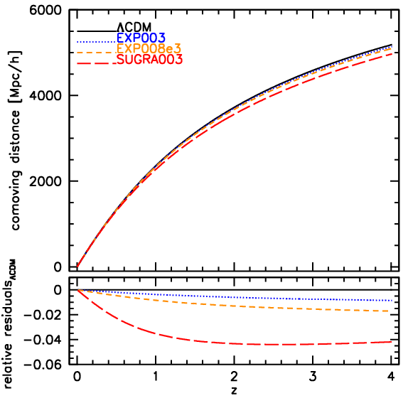
Such variety of scenarios is reflected in the diversity of effects that they determine on both the background expansion history and the linear and non-linear evolution of perturbations. More specifically, the dynamical evolution of the DE scalar field through a matter dominated scaling solution alters the cosmic expansion history with respect to the standard $\Lambda$CDM cosmology in a way that substantially depends on the potential and coupling functions adopted. This is shown in Fig. 1, where we show the comoving distance as a function of redshift for the four models. The bottom panel displays the relative differences of the comoving distances at a given redshift between the cDE models and the reference $\Lambda$CDM. From the figure we can notice that while locally the comoving distances are consistent with each other (due to the same normalisation of Hubble parameter, $H_{0}$, for all the cosmologies), at higher redshifts the cDE models have smaller volumes than $\Lambda$CDM, with a maximum effect for the SUGRA003 cosmology which deviates low from $\Lambda$CDM by about 5 percent already at $z=2$.

At the level of linear density perturbations, the models all predict an enhanced growth rate with respect to $\Lambda$CDM at high redshifts. However, while the EXP003 and the EXP008e3 models show an enhanced growth also at low redshifts, thereby resulting in a larger value of $\sigma_{8}$ at $z=0$, the SUGRA003 cosmology is characterized by a slower growth as compared to $\Lambda$CDM for $z\lesssim 7$ resulting in a comparable value of $\sigma_{8}$ (see the last column of Table 1). The non-linear effects of these models have been studied in several publications based on the outcomes of the CoDECS simulations and range from the impact of cDE on the abundance and structural properties of halos (Baldi, 2012a; Baldi et al., 2011; Cui et al., 2012; Giocoli et al., 2013), on the statistical properties of the large-scale structures distribution (Marulli et al., 2012; Moresco et al., 2014), on the properties of the Inter-Galactic Medium at high redshifts (Baldi & Viel, 2010), and on weak lensing statistics (Beynon et al., 2012; Carbone et al., 2013; Pace et al., 2015). In the present work, we aim at extending the latter analysis by investigating whether a tomographic slicing of the background sources within the light-cone of a 25 square degrees field of view might provide additional information to observationally distinguish the cDE models from the standard $\Lambda$CDM cosmology and possibly the different cDE models from each other.

For our analysis we will make use of the L-CoDECS series consisting of a periodic cosmological box of $1$ Gpc$/h$ aside filled with $2\times 1024^{3}$ particles evolved through collisionless dynamics from $z=99$ to $z=0$. All the models share the same initial conditions at the redshift of the CMB $z_{\rm CMB}\approx 1100$ and have the same cosmological parameters at $z=0$ consistent with the WMAP7 cosmological results (Komatsu et al., 2011), namely $\Omega_{\mathrm{CDM}}=0.226$, $\Omega_{\mathrm{DE}}=0.729$, $h=0.703$, $A_{s}=2.42\times 10^{-9}$, $\Omega_{b}=0.0451$ and $n_{s}=0.966$. The mass resolution is $M_{\rm CDM}(z=0)=5.84\times 10^{10}$ M${}_{\odot}/h$ for CDM particles and $M_{\rm b}=1.17\times 10^{10}$ M${}_{\odot}/h$ for the (collisionless) baryonic particles (see Baldi, 2012c, for a detailed discussion), while the gravitational softening was set to $\epsilon_{g}=20$ kpc$/h$.

3 Lensing Pipeline

In the following sections we will present the procedure we followed in constructing the lens planes from the cosmological simulations, assembling them into light-cones and tracing the paths of light through them.

3.1 Constructing the light-cone: MapSim

Our code for extracting the particles from the simulation’s snapshot files and assembling them into a light-cones is called MapSim. The steps MapSim goes through in constructing a light-cone can be summarized as follows:

• Read in an input parameter file that contains information about the desired field of view, highest source redshift (in this case taken to be $z_{s}=4$) and locations of snapshot files. The number of lens planes required is decided ahead of time in order to avoid gaps in the constructed light-cone. The choice $z_{s}=4$ has been made to better understand where the dynamical evolution of the DE scalar field and the enhanced growth rate – in the different models – start to leave a mark in the weak lensing observables. Notice that at low redshifts the models show a different behaviour: while EXP003 and EXP008e3 continue their enhanced growth, SUGRA003 does not.

• Read in each snapshot file going from the present time to higher redshift snapshots while extracting only the particle positions within the desired field of view. Only a single snapshot is in memory at any time.

• Selection and randomization of each snapshot is done as in Roncarelli et al. (2007). If the light-cone reaches the border of a simulation box before it has reached a redshift range where the next snapshot will be used, the box is re-randomized and the light-cone extended through it again.

• The lensing planes are built by mapping the particle positions to the nearest pre-determined plane, maintaining angular positions, and then pixelizing the surface density using the triangular shaped cloud (TSC) method (Hockney & Eastwood, 1988). The grid pixels are chosen to have the same angular size on all planes. The lens planes have been constructed each time a piece of simulation is taken from the stored particle snapshots; their number and frequency depend on the number of snaphosts stored while running the simulation.

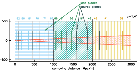
In Fig. 2 we show an illustration of the construction of the light-cone up to redshift $z=1.4$, for the $\mathrm{\Lambda}$CDM model, piling one on top of the others the different portions of the simulation snapshots. The differently colored squares are different realizations using the same randomization method. The rectangles within the squares represents the portion of the simulation snapshot from which the particle density distributions have been taken. The number on the top of them are the id numbers of the corresponding simulation snapshots. The vertical line in the middle of each rectangle indicates the planes onto which the particles are projected for ray-shooting. We remind the reader that to save disk space not all $92$ simulation snapshots have been stored in running the simulation. Up to redshift $z_{s}=4$ we saved $18$ snapshots which are sufficient to consistently model the matter density distribution in our light cones.

The maps were constructed with a $5\times 5$ sq. deg. field of view and an angular resolution of $8.8$ arcsec. For each model we have constructed twenty-five independent realizations, being careful that in each realization the same field of view is selected in the different cosmologies. However, considering the different comoving distance-redshift evolution through the simulation snapshots we have built 22 planes up to redshift $z=4$ for the $\mathrm{\Lambda}$CDM, EXP003 and EXP008e3, while we have 21 planes for the SUGRA003 model. In Table 2 we point out the comoving distances corresponding to redshift $z_{s}=0.5$, 1.4 and 4 for the four models.

Table 2: Comoving distances in Mpc$/h$ for three different source redshifts in the considered cosmological models

model	$z_{s}=0.5$	$z_{s}=1.4$	$z_{s}=4$
$\mathrm{\Lambda}$CDM	1327.27	3000	5179.52
EXP003	1324.56	2999.75	5135.05
EXP008e3	1320.86	2981.97	5091.15
SUGRA003	1297.07	2892.85	4962.47

Figure 3: Convergence maps of a light-cone with aperture 100 arcmin on the x-side, for the four considered models – in each panel top left $\mathrm{\Lambda}$CDM, top right EXP003, bottom left EXP008e3 and bottom right SUGRA003. The three panels refer to different cases: sources located at redshifts $z_{s}=0.5,\,1.4$ and $4$, from top to bottom, respectively. In each map the sticks show the direction of the corresponding field.

3.2 Ray-Tracing through the planes

Once the lens planes are created as described in the previous section the lensing calculation itself is done using the GLAMER lensing code (Metcalf & Petkova, 2013; Petkova et al., 2013). The multiplane ray-tracing method is described in detail in Petkova et al. (2013) so we will only outline the procedure here.

A few definitions are required. If the angular position on the sky is ${\boldsymbol{\theta}}$ and the position on the source plane expressed as an angle (the unlensed position) is ${\boldsymbol{\beta}}$, then a distortion matrix ${\bf A}$ can be defined as

$${\bf A}\equiv\frac{\partial{\boldsymbol{\beta}}}{\partial{\boldsymbol{\theta}}}=\left(\begin{array}[]{cc}1-\kappa-\gamma_{1}&\gamma_{2}-\gamma_{3}\\ \gamma_{2}+\gamma_{3}&1-\kappa+\gamma_{1}\end{array}\right)\ .$$ (3)

The traditional decomposition of this matrix is shown, where $\kappa$ is called the convergence and ${\boldsymbol{\gamma}}$ represents the shear. The torsion, $\gamma_{3}$, represents a rotation which can occur when there are multiple deflection planes. It is of order the shear squared (see Petkova et al., 2013) and according to our numerical calculations, and those of Becker (2013), it is quite small, but it will be retained here for completeness.

Figure 4: Convergence power spectrum of the four considered CoDECS cosmologies for three different source redshifts: $z_{s}=0.5,\,1.4$ and $4$. The shaded grey region encloses the standard deviation of the mean associated to the $\Lambda\mathrm{CDM}$ model on the different $5\times 5$ degree light-cone realisations. In the top panel the solid and dot-dashed curves show the linear and non-linear CAMB predictions for the $\Lambda\mathrm{CDM}$ cosmology respectively. For the non-linear power spectrum prediction we adopt the extended version of the Halofit Model (Smith et al., 2003) from Takahashi et al. (2012). In the bottom panels we present the relative residuals of the convergence power spectra with respect to the $\Lambda\mathrm{CDM}$ cosmology of the three cosmological models – for each of the considered source redshift cases – featuring a direct interaction between the Dark Energy and Dark Matter.

When there is a single lens plane, the convergence can be expressed as a dimensionless surface density,

$$\kappa({\boldsymbol{\theta}})\equiv\frac{\Sigma({\boldsymbol{\theta}})}{\Sigma_{\rm crit}}\ ,$$ (4)

where

$$\Sigma_{\rm crit}\equiv\dfrac{c^{2}}{4\pi G}\dfrac{D_{l}}{D_{s}D_{ls}}$$ (5)

is called the critical density, $c$ is the speed of light, $G$ is Newton’s constant and $D_{l}$ $D_{s}$ and $D_{ls}$ are the angular diameter distances between observer-lens, observer-source and source-lens, respectively. In general, with multiple lens planes, this is not the case however.

The deflection caused by a lens plane, ${\boldsymbol{\alpha}}$, is related to the surface density on the plane, $\Sigma({\bf x})$, through the differential equations

$$\nabla^{2}\phi({\bf x})=\frac{4\pi G}{c^{2}}\Sigma({\bf x})~{}~{}~{},~{}~{}~{}{\boldsymbol{\alpha}}({\bf x})=\nabla\phi({\bf x}).$$ (6)

where the derivatives are with respect to the position on the lens plane. These equations are solved on each source plane by performing a Discrete Fourier Transform (DFT) on the density map, multiplying by the appropriate factors and then transforming back to get a deflection map with the same resolution as the density map. With the same DFT method the shear caused by each plane is simultaneously calculated. Since the rays are propagated between planes using the standard distances in a Robertson-Walker metric which assumes a uniform distribution of matter the addition of matter on each of the planes will, in a sense, over-count the mass in the universe. Without correcting for this the average convergence from the planes will be positive and will cause the average distance for a fixed redshift to be smaller than it should be. To compensate for the implicit density between the planes the ensemble average density on each plane is subtracted. Each plane then has zero convergence on average and the average redshift-distance relation is as it would be in a perfectly homogeneous universe.

After the deflection and shear maps on each plane are calculated the light-rays are traced from the observers through the lens planes out to the desired source redshift. The shear and convergence are also propagated through the planes as detailed in Petkova et al. (2013). GLAMER performs a complete ray-tracing calculation that takes into account non-linear coupling terms between the planes as well as correlations between the deflection and the shear. No weak lensing assumption is made at this stage. The rays are shot in a grid pattern with the same resolution as the mass maps: 5 degrees resolved with 2048 pixels on a side.

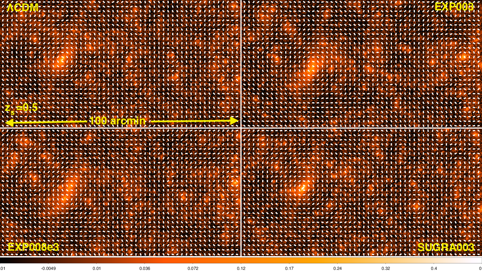
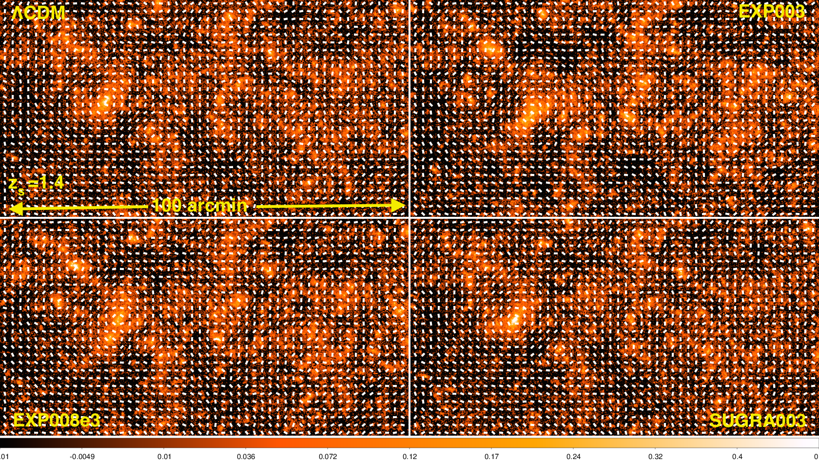
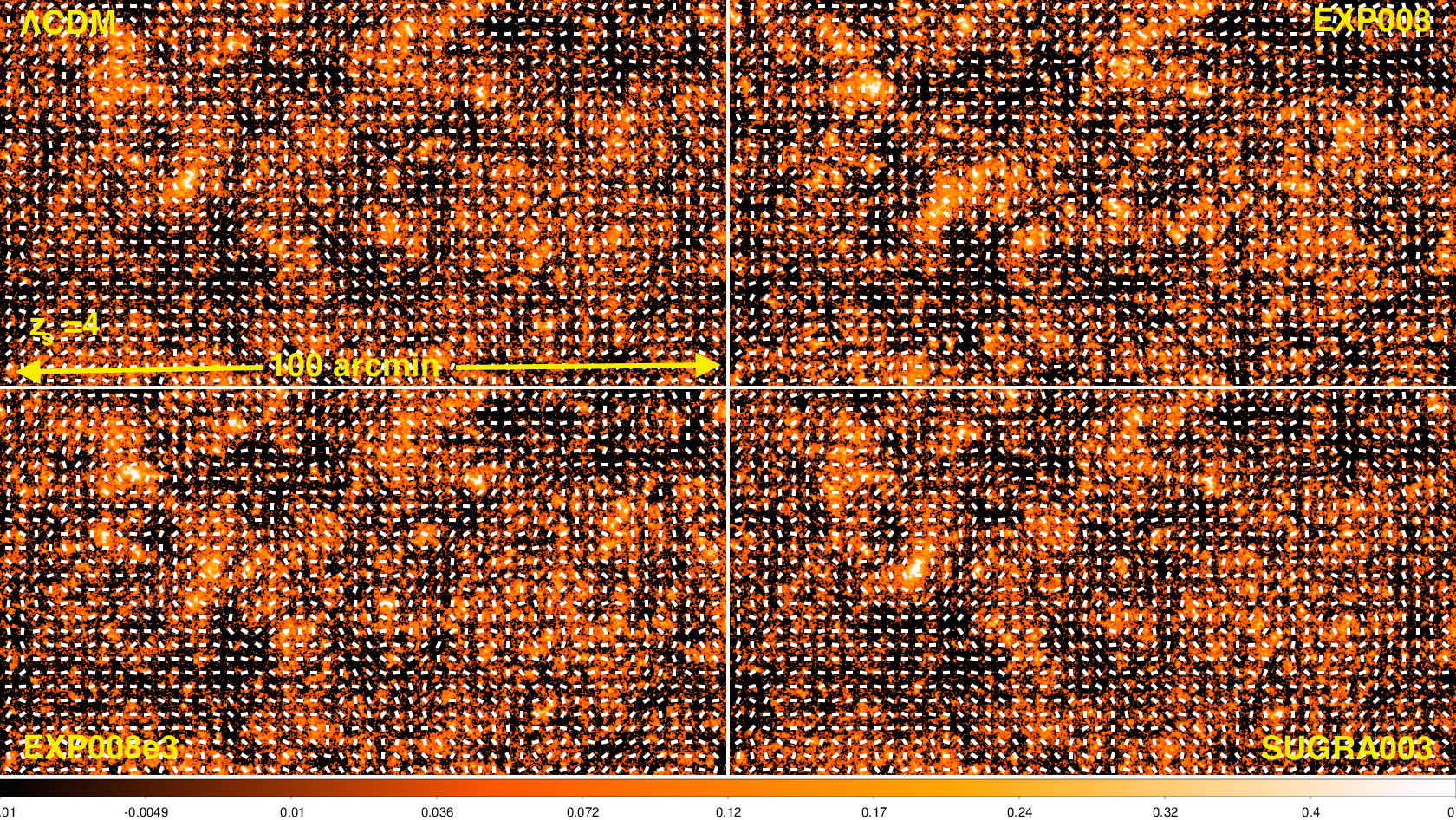
In Fig. 3 we show the convergence maps of the same light-cone realisation extracted from the different models – top left $\mathrm{\Lambda}$CDM, top right EXP003, bottom left EXP008e3 and bottom right SUGRA003. We show the maps for sources located at three fixed redshifts: $z_{s}=0.5$, 1.4 and 4 from top to bottom, respectively. The sticks in each panel indicate the directions of the corresponding shear field. As discussed in Cui et al. (2012) and Giocoli et al. (2013), we immediately notice that the density distribution differs in cDE models from $\mathrm{\Lambda}$CDM due to a difference in the growth as a function of redshifts. The top panels show the presence in the field of view of a cluster, at redshift $z<0.5$, which, while it appears “assembled” and with a single peak in the $\mathrm{\Lambda}$CDM and the SUGRA003 models, it is less evolved, showing multiple components, in EXP003 and EXP008e3. The intermediate and the high redshift maps also exhibit differences mainly because of differences in the evolution of the power spectrum normalisation and non-linear structure formation.

3.3 Analytic methods

An approximation is commonly used to calculate the convergence power spectrum that avoids the complications discussed in the previous two sections. The convergence can be calculated by adding up the single plane convergences, equation (6), along an unperturbed light-ray, the Born approximation. This results in the expression

$$\kappa(z_{s},\boldsymbol{\theta})=\dfrac{3H^{2}_{0}\Omega_{m}}{2c^{2}}\int_{0}^{w(z_{s})}\mathrm{d}w\dfrac{D(z)D(z,z_{s})}{D(z_{s})a(z)^{2}}~{}\delta\left(D(z)\,\boldsymbol{\theta},z\right)\ ,$$ (7)

where $w$ is the radial comoving distance, $a\equiv(1+z)^{-1}$ is the scale factor and $\delta({\bf x})\equiv(\rho({\bf x})-\overline{\rho})/\overline{\rho}$ is the density contrast. The angular power spectrum of $\kappa$ in the small angle limit is then found to be

$$P_{\kappa}(l)=\dfrac{9H_{0}^{4}\Omega_{m}^{2}}{4c^{4}}\int_{0}^{w_{s}}\mathrm{d}w\left(\dfrac{D(z,z_{s})}{D(z_{s})a(z)}\right)^{2}P_{\delta}\left(l\dfrac{a(z)}{D(z)},z\right)$$ (8)

(Kaiser, 1992). Either an analytic model for the density power spectrum, $P_{\delta}(k,z)$, or a power spectrum taken directly from a simulation can be inserted into eq.(8).

In the following sections we will contrast our direct calculations with some analytic models using this approximation. For some applications this approximation is adequate, but in new situations and for particular statistics it needs to be checked against simulations.

4 Results

4.1 Convergence Power Spectrum

Figure 5: Left panel: ratio between the convergence power spectrum computed at different source redshifts – as indicated in the labels – and the one at $z_{s}=0.5$ for each cosmological model. Right panel: rescaled cross power spectra between redshift $z=0.5$ and $z_{2}$ – as indicated in the labels – for the different models, computed from the lensing maps. All the cross spectra have been rescaled with respect to the $\mathrm{\Lambda}$CDM prediction. This is why the correlation parameter on the right can be greater than one. Different line styles and colors are as in Fig. 4.

In the real (angular) space, a direct measurement of weak lensing is the two-point shear correlation functions $\xi_{+}$ and $\xi_{-}$ that can be obtained by averaging over galaxy pairs with angular separations $|\boldsymbol{\theta}_{i}-\boldsymbol{\theta}_{j}|$ within a bin $\theta$:

$$\xi_{\pm}(\theta)=\dfrac{\sum_{ij}w_{i}w_{j}\left[\epsilon_{t}(\boldsymbol{\theta}_{i})\epsilon_{t}(\boldsymbol{\theta}_{j})\pm\epsilon_{\times}(\boldsymbol{\theta}_{i})\epsilon_{\times}(\boldsymbol{\theta}_{j})\right]}{\sum_{ij}w_{i}w_{j}}\ ,$$ (9)

where the measured galaxy ellipticity measurements $\epsilon_{t}$ and $\epsilon_{\times}$ are the tangential and cross components with respect to the line connecting the pair, respectively. The weights $w$ are obtained from the galaxy shape measurement pipeline (Bernstein & Jarvis, 2002; Bridle et al., 2010; Kacprzak et al., 2012; Miller et al., 2013). These two-point shear correlation functions can be calculated from the convergence power spectrum by the relation:

$$\xi_{+/-}=\dfrac{1}{2\pi}\int_{0}^{\infty}\mathrm{d}l~{}lP_{\kappa}(l)J_{0/4}(l\theta)\,,$$ (10)

where $J_{0}$ and $J_{4}$ are the Bessel functions and we have set the B-mode power spectrum to zero because lensing generates only E-modes in the weak lensing limit.

Figure 6: Left panel: histograms of the convergence values in one realization of the $\mathrm{\Lambda}$CDM model, considering sources at $z_{s}=1.4$. The solid black histogram shows the case for the map resolution used throughout this paper ($8.8$ arcsec pixels). The short dashed green, long dashed magenta and dot-dashed blue histograms show the PDF of the maps degraded by a factor of 2, 4 and 8, respectively. Right top panel: convergence power spectra of these maps. Right bottom panel: the ratios of the power spectra with different resolutions with respect to the highest resolution one.

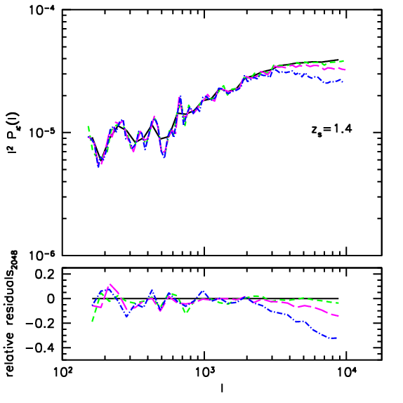
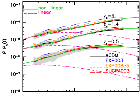
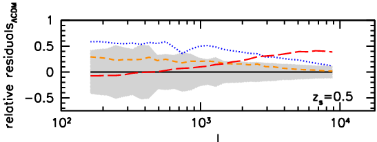
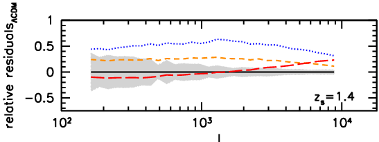
In Fig. 4 we show the convergence power spectrum up to $l\approx 10^{4}$ measured in the four cosmologies, considering sources at three different redshifts: $z_{s}=0.5$, 1.4 and 4. The curve referring to each model represents the average over all the light-cones. For the $\mathrm{\Lambda}$CDM case the shaded region encloses the standard deviation of the mean associated to the different realizations. The $l_{min}$ considered corresponds to the minimum resolvable in the assumed field of view. In the same figure we also show the predictions obtained by inserting into equation (8) analytic models for the linear and the non-linear power spectrum, namely the Halofit Model (Smith et al., 2003) from Takahashi et al. (2012) implemented in CAMB (Lewis et al., 2000). As shown in Pace et al. (2015) – where they consider the matter density distribution only up to redshift $z_{s}=1$ – the EXP003 model has much more power than the $\mathrm{\Lambda}$CDM with the largest difference being on small scales and increasing with the source redshift. Interestingly, for the SUGRA003 model, the power spectrum is below $\mathrm{\Lambda}$CDM for low multipoles and above it for high multipoles. This is a result of the fifth force term in the dark matter-dark energy coupling which drives rapid structure formation at high redshift, but slows it down at lower redshift. The SUGRA003 and the $\mathrm{\Lambda}$CDM power spectra intersect at about $l\sim 10^{3}$, slightly decreasing with the source redshifts. From Fig. 4 we also see that the EXP008e3 model has about 15-25 percent more power than $\mathrm{\Lambda}$CDM at all scales and source redshifts, a signature of its growth rate being maintained over the whole redshift range. As obtained by the tomographic analysis performed by Pace et al. (2015), where only the ratio of the power spectra for sources at redshift $z_{s}=2$ and $z_{s}=1$ has been considered, we confirm that the small differences they find at very high $l$ in the coupled models, and particularly in the bouncing model SUGRA003, are actually present and are much clearer in our high-resolution ray-traced maps. The same behaviour of the power spectra we find has also been noticed and discussed by Carbone et al. (2013) using ray-tracing technique to compute the CMB lensing maps; however also Carbone et al. (2013) are not able resolve the small scale features of the coupled DE-DM models because the angular resolution on their maps is more than a factor of ten lower than ours.

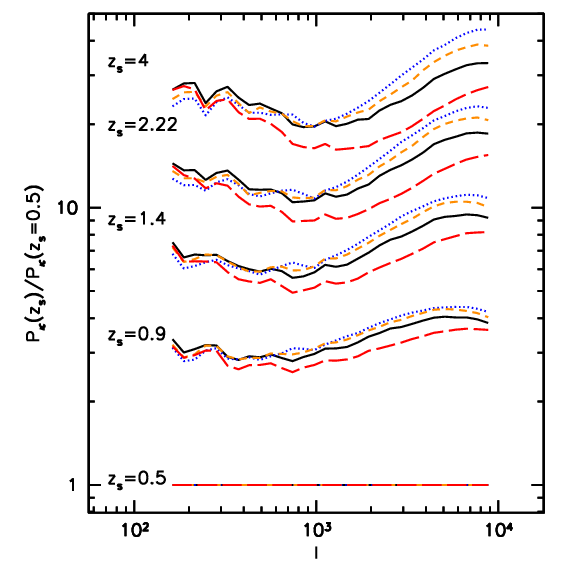
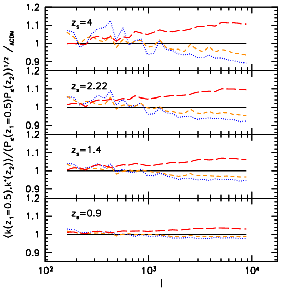
Clearly weak lensing tomography, i.e. the study of the weak lensing signal as a function of the source redshift, can be an important tool for studying these differences in the evolution of structure with redshift that occur in different coupled Dark Energy models. Fig. 5 shows this more clearly. In the left panel we display the ratio between the convergence power spectrum computed at five different source redshifts and the one computed for sources located at $z_{s}=0.5$; line styles and colors are the same as in Fig. 4. For EXP003 and EXP008e3 the ratios tend to lie above the $\mathrm{\Lambda}$CDM one, but for SUGRA003 it stays below. This is a result of structures in the SUGRA003 model evolving less rapidly at late times while in the EXP003 and EXP008e3 models they evolve more rapidly. The difference between the models is most evident at small scales as a consequence of non-linear structure formation. The right panel of Fig. 5 show the rescaled cross-spectra between the convergence at different redshifts within the same light-cone. High correlation indicates that the lensing is being caused by the same objects. Interestingly, SUGRA003 has more correlations at small scales and less at large scales, while the other models have the opposite trend, due to an enhancement of their growth rate at high redshifts and to a depletion at low redshifts with respect to the $\mathrm{\Lambda}$CDM one. We remind the reader that the growth rate in EXP003 and EXP008e3 is always enhanced with respect to the standard model causing a higher $\sigma_{8}$ at the present time.

Figure 7: Left panel: $\sigma_{8}$ as a function of the source redshift, obtained by fitting the corresponding convergence power spectrum for each cosmological model, fixing the total mass density parameter $\Omega_{m}$ to its true value in the simulation. The colored points show the value of $\sigma_{8}$ at the present time interpolated from linear theory: blue triangle (EXP003) , orange diamond (EXP008e3), red cross (SUGRA003) and black dot ($\mathrm{\Lambda}$CDM). Right top panel: convergence power spectra for sources at redshift $z_{s}=4$ as measured from the light-cones in the four cosmological models. As in previous figures solid, dotted, dashed and dot-dashed lines correspond to $\mathrm{\Lambda}$CDM, EXP003, EXP008e3 and SUGRA003, respectively. The corresponding solid colored curves represent the best $\mathrm{\Lambda}$CDM power spectra obtained fixing the total matter content and varying $\sigma_{8}$. Bottom right panel: the ratio between the convergence power spectrum with the best $\sigma_{8}$ and the one obtained using $\sigma_{8}(z=0)$, i.e. the interpolated value using linear theory (Baldi, 2012c) is shown for the three cDE models.

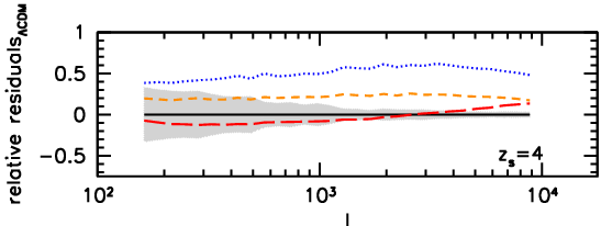
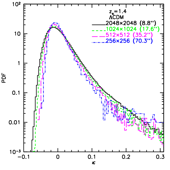
The pixel resolution of our maps ($8.8$ arcsec in all cases) will have some impact on the accuracy of the lensing statistics calculated. In particular the pixelation tends to smooth out peaks and reduce the power on small scales (Takahashi et al., 2011; Pace et al., 2015). To investigate how our pixelation might be affecting the results we constructed the pixel Probability Distribution Function (PDF) of the convergence map as shown in Fig. 6 for one realisation of the $\mathrm{\Lambda}$CDM model with sources at $z_{s}=1.4$. The different line styles and color histograms show the PDF when the original map has been pixel-degraded by a factor of $2$, $4$ and $8$ – see the figure caption for more details. It can be seen that increasing the pixel size reduces the number of very high and very low $\kappa$ pixels as expected. The impact this has on the convergence power spectrum is shown in the right hand panel of Fig. 6, where the power spectra for different resolutions are plotted. In the bottom right hand panel are the relative residuals with respect to the original, highest resolution map. These figures show that reducing the map resolution by a factor of two causes small differences of only a few percent in the power spectrum relative to the original map for $l\lower 2.15277pt\hbox{$\;\buildrel<\over{\sim}\;$}5\times 10^{3}$. The discrepancies become larger for the maps degraded by a factor of four and eight. We conclude that our calculations are not affected by pixelation for $l\lower 2.15277pt\hbox{$\;\buildrel<\over{\sim}\;$}5\times 10^{3}$ above few percent level.

It has been shown in this section that the evolution of the density power spectrum in different coupled dark energy models will cause significant changes to the convergence power spectrum as a function of source redshift. These differences from $\Lambda$CDM can be positive or negative at a particular source redshift and they can be scale dependent. In the following sections we will investigate some other statistics that might be observationally more practical in terms of direct measurements and noise estimations.

4.1.1 Impact on the measured normalisation of the power spectrum for sources at different redshifts

As noted previously, the coupled DM-DE models affect both the power spectrum normalisation and the small scale non-linear behaviour of structure formation when compared with the $\Lambda$CDM model. One way to see this is through the impact on measurements of the power spectrum normalisation. The power spectrum normalisation will be quantified by the standard $\sigma_{8}$ parameter which is the variance of the mass overdensity density within a sphere of radius $8~{}h^{-1}$ Mpc at redshift zero with only the linear evolution of the power spectrum taken into account. When $\sigma_{8}$ is measured using data at redshifts larger than zero a correction factor that is cosmology dependent must be applied to translate the normalisation to $z=0$. If the underlying cosmology assumed in doing this procedure is the correct one then $\sigma_{8}$ will not depend on the source redshift. In this section we investigate what would happen if a $\Lambda$CDM cosmology is assumed while the true cosmology corresponds to one of our coupled dark energy models. This exercise will help us gain some insight on when during cosmic history these models leave most of their imprints on the lensing power spectrum.

Figure 8: Top panels: variance of the convergence field smoothed with a compensated aperture filter as a function of the smoothing scale $\theta$, for sources at three different redshifts: $z_{s}=0.5,\,1.4$ and $4$, from left to right. Bottom panels: relative residuals as a function of the smoothing scale with respect to the measurements in the $\mathrm{\Lambda}$CDM model. The grey shaded region represents the rms of the variance computed on the different realizations of the $\mathrm{\Lambda}$CDM light-cone. In the right panel, for sources at $z_{s}=4$, we also show predictions from linear and non-linear theory. For the other source redshifts the agreement is analogous to this one.

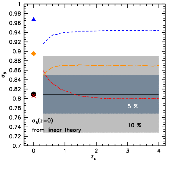
The left hand panel of Fig. 7 shows the recovered $\sigma_{8}$ values as a function of the different source redshifts for the four cosmological models while assuming $\mathrm{\Lambda}$CDM. We measure $\sigma_{8}$ integrating the non-linear power spectrum (see e.g. Lewis et al., 2000; Takahashi et al., 2012) up to the different considered source redshifts assuming the $\mathrm{\Lambda}$CDM model; in this way the $\sigma_{8}$ value is directly related to the measurement of the growth factor associated to a $\mathrm{\Lambda}$CDM Universe. Line styles and colors are the same as in Fig. 4, the shaded light grey and grey regions indicate $5$ and $10$ percent accuracies in the measurement of $\sigma_{8}$ for the $\Lambda$CDM case. Also shown are the true $\sigma_{8}$ values – interpolated using linear theory (Baldi, 2012c) – for each model. In the case of $\mathrm{\Lambda}$CDM the correct value is recovered, but in the other models incorrect $\sigma_{8}$ values are recovered and they change as a function of source redshift. Such behaviour would therefore signal a failure of the underlying $\Lambda$CDM assumption. In EXP003 and EXP008e3, $\sigma_{8}$ is underestimated, while the opposite is true in SUGRA003 for some of the source redshift range. These trends are due to the different evolution of the growth factor and of the Hubble function in the coupled DM-DE models – see Fig. 1 and Fig. 2 in Baldi (2012c). It is interesting to note that for the three coupled models we never obtain the value of $\sigma_{8}$ interpolated from linear theory at the present time. This means that when fitting the convergence power spectrum of the coupled DM-DE models both projection effects and non-linearities contribute to the measured $\sigma_{8}$.

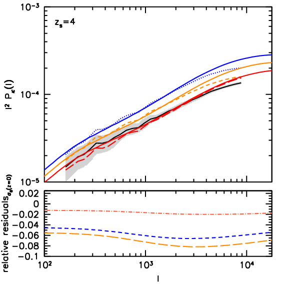
In the right hand panel of Fig. 7 we show the measured convergence power spectrum in the different light-cone simulations for sources at $z_{s}=4$ – solid, dotted, dashed and dot-dashed refer to $\mathrm{\Lambda}$CDM, EXP003, EXP008e3 and SUGRA003, respectively. For the three coupled DM-DE models we display best fitting theoretical convergence power spectra obtained by assuming we live in a $\mathrm{\Lambda}$CDM universe. In the bottom panel we present the relative deviation of the theoretical convergence power spectrum computed with the best $\sigma_{8}$ and the one linearly interpolated from theory at $z=0$. While for SUGRA003 model the relative deviation is of the order of $1-2\%$, for both EXP003 and EXP008e3 it manifests larger values.

These results indicate that, if sufficient accuracy is attained, measuring $\sigma_{8}$ from shear maps as a function of redshift would lead to inconsistencies were one of these coupled dark energy models the correct one. To observe these effects will require large amounts of very accurate data of the kind that will be provided by future wide surveys, like the Euclid space mission (Laureijs et al., 2011). An additional complication not taken into account here is that weak lensing studies are generally sensitive to a combination of the power spectrum normalisation, $\sigma_{8}$, and the total density of matter, $\Omega_{m}$, in the combination $\sigma_{8}\left(\Omega_{m}/0.25\right)^{\alpha}$ where $\alpha$ is dependent on the weak lensing statistic used: $\alpha=0.46$, $0.53$ and $0.64$, for the shear two-point correlation function, the shear in a top-hat or aperture mass, respectively (Fu et al., 2008; Kilbinger et al., 2013, see also a more extended discussion in the next section). However, $\Omega_{m}$ is likely to be well constrained by other observations such as the CMB.

4.2 Other weak lensing statistics

Other statistics of the convergence field besides the power spectrum may help to probe the non-Gaussian nature of the probability distribution function of gravitational lensing observables. In particular, statistics like the variance and the skewness in a top-hat or compensated filter represent interesting tools to constrain cosmological parameters and the dark energy evolution as a function of redshift (Fu et al., 2008; Kilbinger et al., 2013; Kitching et al., 2014). In this context, multi-plane lensing simulations are important tools to compute the predicted variance and skewness of the shear or convergence field, both for standard and non-standard models. In particular, the skewness in aperture is somehow independent of the normalization of the power spectrum and represents a strong indicator of the evolution of $\Omega_{m}$ as a function of redshift (Schneider et al., 1998).

The interpretation and modelling of the lensing signals due to large scale structures requires a precise understanding of the high-order statistics of the lensing field (Sato et al., 2009). Several cosmological analyses have been done by studying the mass aperture variance and the skewness as a function of the smoothing angle $\theta$, adopting a top-hat or a compensated aperture filter. These measured quantities have the advantage that they can be directly compared with the theoretical predictions extracted from the convergence power spectrum. However, a good model of the signal on small scales, where the non-linear effects start to dominate, is of fundamental importance to interpreting observational data. Since the top-hat shear rms between different CoDECS models, but only at $z_{s}=1$, has been studied by Pace et al. (2015), we will present and discuss in this section the aperture-mass dispersion and the associated skewness for three different source redshifts.

The variance of the filtered shear field as a function of the filter size contains the same information as the power spectrum, but the filter can be made to have compact support and additional practical advantages (Sato & Nishimichi, 2013). They can also have a different sensitivity to the cosmological model and be particularly dependent on non-linear structure formation. In addition, the skewness and higher-order statistics can be easily defined and interpreted for the filtered shear field. We will investigate a particular choice of filter called the compensated aperture filter:

$$Q_{\theta}(\vartheta)=\dfrac{6}{\pi\theta^{2}}\left(\dfrac{\vartheta}{\theta^{2}}\right)\left(1-\dfrac{\vartheta^{2}}{\theta^{2}}\right)\,$$ (11)

with support $\vartheta=[0,\theta]$. In Fourier space it is

$$W_{ap}=\dfrac{\sqrt{276}J_{4}(\xi)}{\xi^{2}}$$ (12)

as Fourier counterpart (Harnois-Déraps et al., 2012). It has the attractive property of being well-localized in Fourier space near wavenumber $l\sim 5/\theta$. We apply this filter in Fourier space with zero-padding to reduce boundary effects. Since the average value of the convergence on each plane is zero, the variance across the map, typically indicated as $\langle M_{Ap}^{2}\rangle$, can be computed from the convergence power spectrum performing the following integral:

$$\langle k^{2}\rangle_{Ap}=\langle M_{Ap}^{2}\rangle=\dfrac{1}{\left(2\pi\right)^{2}}\int\mathrm{d}l\,lP_{\kappa}(l)W^{2}_{Ap}(l\theta)\,.$$ (13)

Similarly, it is possible to define the large scale structure noise (Hoekstra, 2003) adopting a different compensated filter (see Appendix A for more discussion about this).

Figure 9: As Fig. 8, but for skewness of the convergence field.

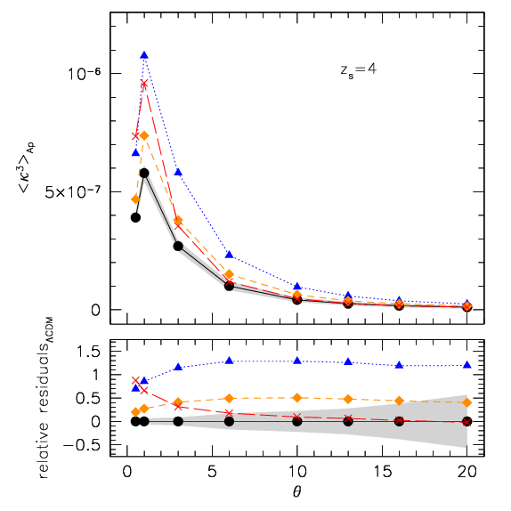
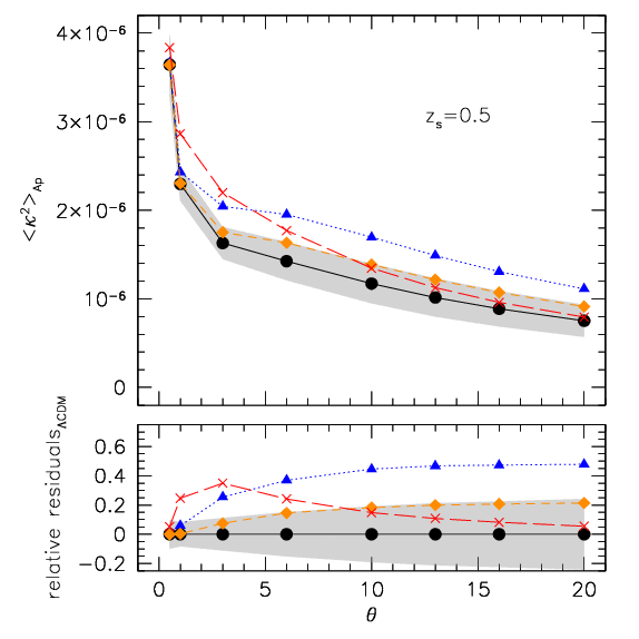
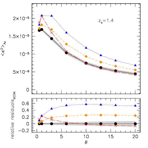
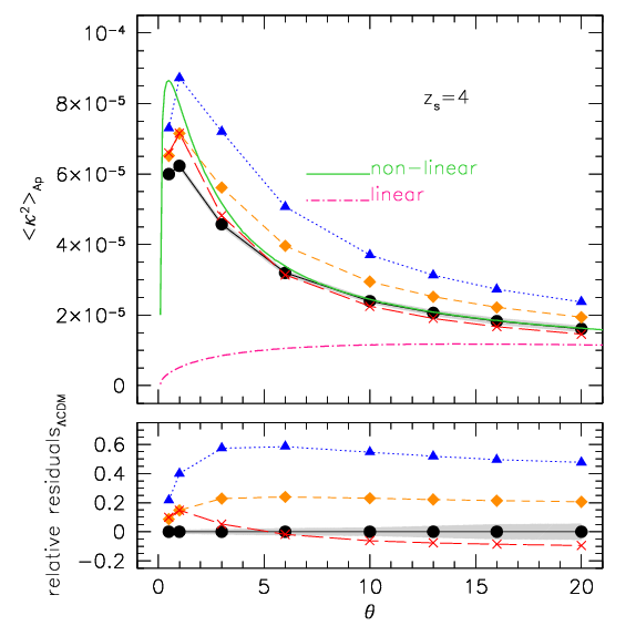
In Fig. 8, we show the variance of the convergence field as a function of the smoothing scale $\theta$ with this filter. The different line styles and colors refer to the four considered cosmological models and the shaded grey region encloses the rms of the measurement performed in the different realizations of the $\mathrm{\Lambda}$CDM light-cones. The measurements are presented for three source redshifts: $z_{s}=0.5$, 1.4 and 4. The bottom panels show the relative residuals of the measurements in the different coupled models with respect to the $\mathrm{\Lambda}$CDM ones. We notice that the variance of the measurement in the $\mathrm{\Lambda}$CDM model decreases as a function of the source redshift, as expected from the evolution of the clustering of the dark matter in the Universe. While at low redshifts the Universe is more clustered and so we may trace rays through clusters and voids – enhancing the variance of the measurements in different realisations, at high redshifts the Universe is more homogenous and so the variance through different realisations is expected to be smaller, as we confirmed in Fig. 8.

To demonstrate how much of this signal depends on non-linear structure formation we show $\langle M^{2}_{Ap}\rangle$ calculated with only the linear power spectrum in the right hand panel of Fig. 8 for $z_{s}=4$ in the $\mathrm{\Lambda}$CDM model. It can be seen that non-linear structure formation has a dominant role below $\theta\simeq 20$ arcmin.

The agreement between non-linear theoretical predictions and our simulations for $\mathrm{\Lambda}$CDM are quite good aside from limitations in the simulations at small scales due to numerical mass and force resolution limitations. As with the power spectrum, the deviations from $\mathrm{\Lambda}$CDM in Fig. 8 are positive for EXP003 and EXP008e3 (by about 50 and 20 percent – as for the convergence power spectrum). For SUGRA003, $\langle M^{2}_{Ap}(\theta)\rangle$ is larger than for $\mathrm{\Lambda}$CDM at small $\theta$ and becomes smaller at large scales mirroring the behaviour in Fig. 4. This trend is a consequence of a slightly lower $\sigma_{8}$ governing the large $\theta$ behaviour while for small scales the boost in variance comes from differences in the structure of halos: in SUGRA003 haloes are more concentrated and have more substructures mainly at low redshifts (as was shown e.g. by Giocoli et al., 2013).

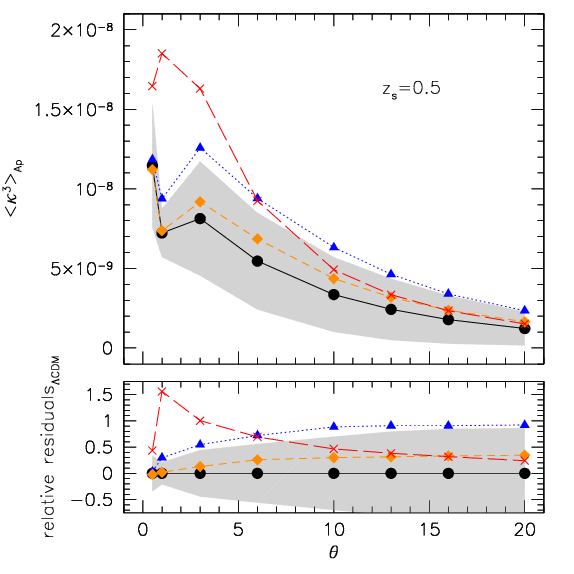
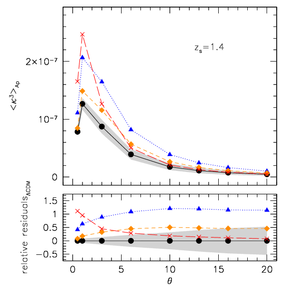
The filtered variance’s strong dependence on non-linear structure leads one to think that the skewness of the filtered convergence map might be a good discriminator between models. The skewness is plotted in Fig. 9 as a function of $\theta$, for all the cosmological models, and once again for three source redshifts. As in the case of the variance, the measurements in the EXP003 and EXP008e3 cosmologies are larger than those in $\mathrm{\Lambda}$CDM, but with the relative residuals that are a factor of two larger than for the variance. In addition, for large angles the relative residuals between $\mathrm{\Lambda}$CDM and SUGRA003 are very small but increase for small $\theta$, a signature of the higher small scale clustering present in this case, the high concentration of haloes and their clumpiness. For a fixed angular scale the difference becomes larger for smaller source redshift owing to the build up of non-linear structure at late times in the SUGRA003 model. These difference between models are more evident here than for the variance.

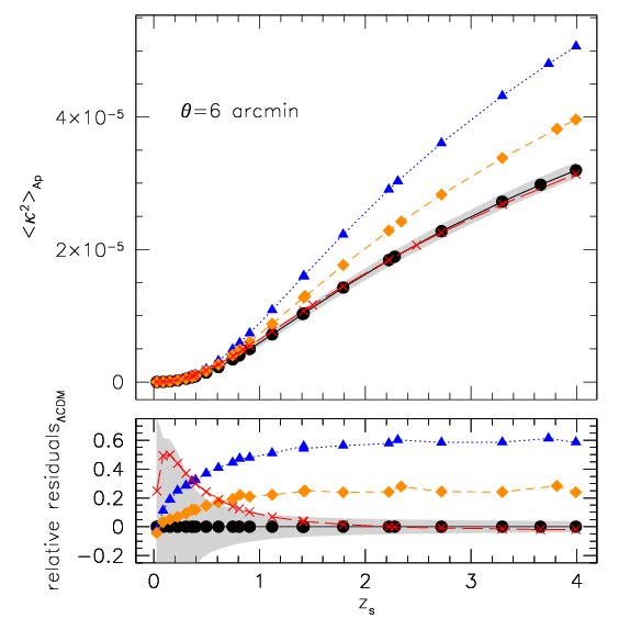
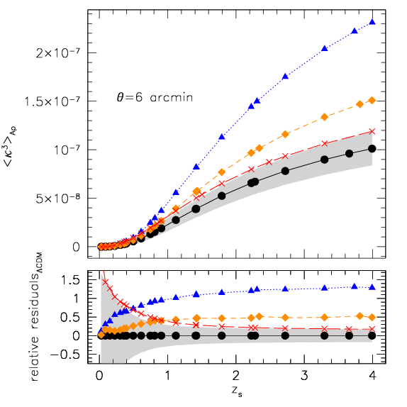
In Fig. 10 we show the variance (left) and the skewness (right) of the convergence field as a function of the source redshift while fixing the scale of the filter to 6 arcmin which is comparable to the typical scale of the central region of galaxy clusters at intermediate redshifts. The bottom panels again show the residuals of the measurements with respect to $\mathrm{\Lambda}$CDM. Both the variance and the skewness grow as a function of the source redshifts because of the increased path lengths and the additional structure along the paths. For $z_{s}>0.5$ all the models tend to present a constant bias with respect to $\mathrm{\Lambda}$CDM: positive in EXP003 and EXP008e3 while almost vanishing in the bouncing model SUGRA003. Note that the relative difference in the skewness is almost double than in the variance. While the behaviour of the bouncing model SUGRA003 is within the rms of the $\mathrm{\Lambda}$CDM measurements, the EXP003 and EXP008e3 are quite distinct with a positive bias of about $60$ percent and $20$ percent for the variance and $120$ percent and $50$ percent for the skewness for $z_{s}>0.5$.

The behaviour of the variance and skewness of the filtered convergence field highlights the possibility of using sources at different redshifts and with different smoothing scales to investigate the coupling between the dark components of the universe.

Figure 10: Variance (left panel) and skewness (right panel) of the convergence field smoothed with a compensated aperture filter with $\theta=6$ arcmin as a function of the source redshifts. The bottom panels show the relative residuals of the variance and the skewness with respect to the $\Lambda\mathrm{CDM}$ measurements. The shaded grey region represents the rms of the moments computed on the different realizations of the $\Lambda\mathrm{CDM}$ light-cones.

4.3 Probability distribution function from source redshift distributions

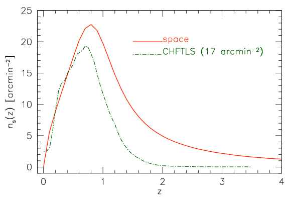
In previous sections we have discussed the results for the variance and the skewness of the convergence field for sources located at different fixed redshifts. In this last section we explore the one-point distribution function of convergence, shear and magnification given instead a source redshift distribution. We do this in order to understand whether the simple one-point statistics of the lensing field, and which source redshift distribution can help us to understand the non-Gaussian nature of the fields in the different cosmological models. In our analysis we consider two different source redshift distributions that typically correspond to a ground- and a space-based weak lensing survey. For the ground-based case we adopt the source density as a function of redshift as computed by Kilbinger et al. (2013) – the data points are publicly available on the CFHTLenS webpage – while for the space-based we consider the parametrization adopted by Boldrin et al. (2012) which has been extracted from a Euclid-like observation of the Hubble Ultra Deep Field performed with the code SkyLens (Meneghetti et al., 2008). In the top left panel of Fig. 11 we show the two adopted source redshift distribution normalizing the CFHTLS one to have a total density of sources of about $17$ galaxies per arcmin². What is most evident about the two is that the high redshift tail in the space-based observation extends to higher redshifts while in the ground-based case there are almost no galaxies above $z=2$. In order to extract the convergence and shear catalogues from one light-cone realization we proceed in the following way: (i) given a source redshift distribution we compute the number of expected sources in a redshift interval $\mathrm{d}z$ that corresponds to the difference in comoving distance between two source planes; (ii) for each $\mathrm{d}z$ we randomly assign to each source both a redshift and an angular position in the field of view. We do not take into account any clustering of the sources which should no be important for our purpose. The corresponding lensing quantity (convergence or shear) is then linearly interpolated in redshift considering the values computed between two consecutive planes at the corresponding angular position of the source. The other panels of Fig. 11 show the convergence, shear and weak lensing magnification for the different $\mathrm{\Lambda}$CDM light-cone realizations, each randomly sampled twenty-five times with the according $n(z_{s})$. From the figure we notice that because the two adopted source redshift distributions have different shapes, mainly in the intermediate and high redshift tail, the one-point lensing statistics from the same simulated light-cones tend to be different. While the shape of the convergence and the magnification are broadened going from ground- to space-based observations, the shear distribution is shifted toward larger values.

Figure 11: Top left: source redshift distribution expected for space- and ground-based observations. Top right, bottom left and bottom right PDF of convergence, shear and magnification extracted from the twenty-five $\mathrm{\Lambda}$CDM light-cones randomly sampled eight times with the corresponding source redshift distribution. The various color and line style histograms refer to the different considered cosmologies (see Fig. 4), the shaded grey region encloses the rms of the measurement performed in the different light-cone realizations in the $\mathrm{\Lambda}$CDM model.

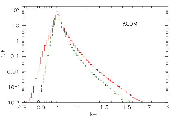
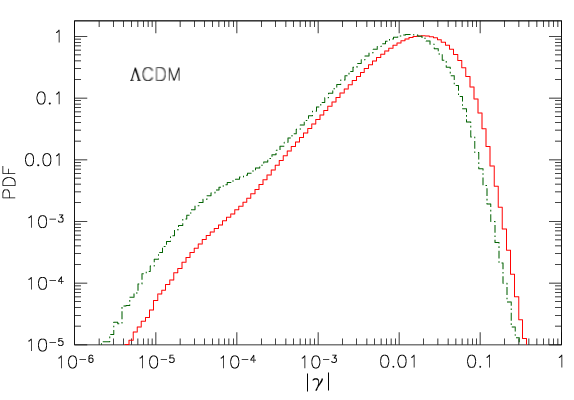
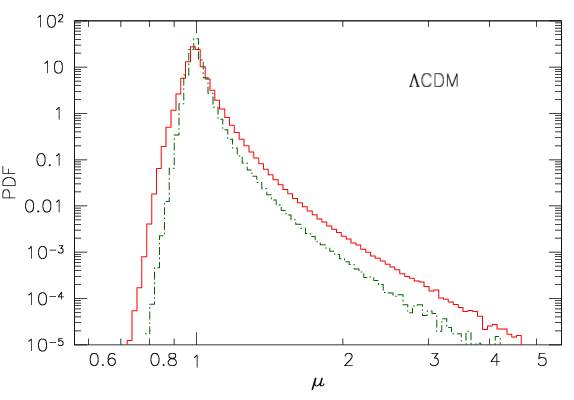
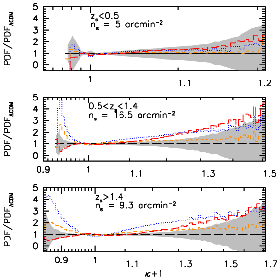
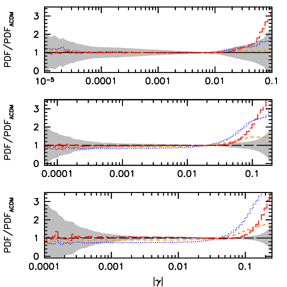
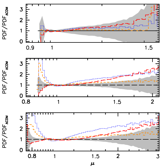
In Fig. 12 we show the expected convergence, shear and magnification probability distributions assuming a space based source redshift distribution for the four cosmologies, rescaled with respect to the $\mathrm{\Lambda}$CDM one. In comparison to Pace et al. (2015) we notice that our distributions are realistically more extended in the high-value tails because of the different way adopted in doing the ray-tracing, and of the larger resolution with which the maps are resolved. While in Fig. 6 by Pace et al. (2015) the one-point statistic manifests itself mainly in the different initial power spectrum normalisation of the coupled models, in Fig. 12 it is possibile to observe also a more pronounced distinction in the high value tails. Particularly, in both the PDF of the convergence and the magnification, the small scale clustering and the high halo concentration in SUGRA003 model raise the high value distribution tails. This is also evident in the shear distributions where both SUGRA003 and EXP003 are well outside the rms of the $\mathrm{\Lambda}$CDM distribution for $\gamma>0.075$. The situation is different for the corresponding PDF extracted from the same light-cones considering a ground-based source redshift distribution, not shown here. First we notice that the source densities in the intermediate and the high redshift bins reduce to $11.2$ and $0.8$ $\mathrm{arcmin}^{-2}$, respectively, and that the SUGRA003 model is enclosed within the rms of the $\Lambda$CDM for large values. In this case only EXP003 appears distinguishable from $\Lambda$CDM. The signature of enhanced high redshift growth in the considered models is much less distinguishable with the ground-based lensing survey than it is with a space based survey, as also discussed in Beynon et al. (2012).

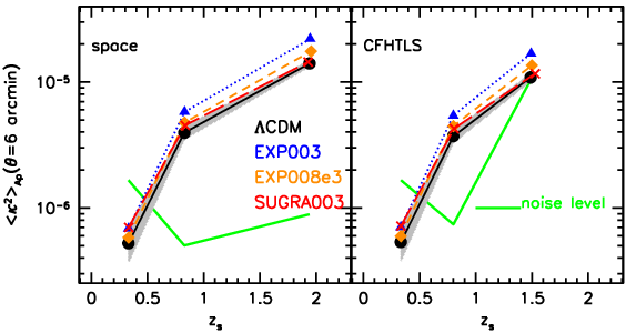
In Fig. 13 we display the variance of the convergence field computed from different light-cone realisations in three redshift bins for a space (left) and ground-based (right), assuming a CFHTLS source redshift distribution. Black, blue, orange and red colors refer to the $\Lambda$CDM, EXP003, EXP008e3 and SUGRA003 models, respectively. In each panel we also show with a green solid line the noise level in the three redshift bins related to the intrinsic ellipticity distribution $\sigma_{\epsilon}=0.25$ and to the corresponding source number density $n_{g}$ contained in the aperture filter (Schneider et al., 1998; van Waerbeke, 2000). This is the noise for a 25 square degree field. Neglecting systematic errors, the noise for a larger survey will go down by roughly a factor of one over the square root of the survey area. From this plot it can be seen that a ground based survey will have difficulty distinguishing between the models, but that a survey like Euclid would be expected to clearly distinguish between them.

Figure 12: PDFs of convergence (left column), shear (central column) and magnification (right column) extracted from the light-cones of the different cosmologies rescaled with respect to the $\mathrm{\Lambda}$CDM one, assuming a space based source redshift distribution. Rows refer to different intervals for the source redshifts: $z_{s}<0.5$, $0.5<z_{s}<1.4$ and $z_{s}>1.4$, from top to bottom. Each light-cone has been randomly sampled eight time with the according source redshift distribution.

Figure 13: Variance of the convergence field computed within the different light-cone realisations and cosmologies adopting a space and a ground-based (CFHTLS) source redshift distribution. Different data points and colors are the same as in Fig. 10. The solid (green) line represents the corresponding noise level associated to the intrinsic galaxy ellipticity distribution and the source number density. This noise level is for a 25 square degree field.

5 Summary and Conclusions

Several studies have been conducted to understand which observables are most suitable to investigate coupled Dark Energy cosmologies (Beynon et al., 2012; Giocoli et al., 2013; Carbone et al., 2013; Pace et al., 2015). Our aim here was to extend the ray-tracing analyses of Carbone et al. (2013) and Pace et al. (2015) by investigating whether a tomographic slicing of the background sources within high resolution simulated light-cones might provide additional information to distinguish coupled dark energy models from the standard $\Lambda$CDM cosmology and possibly the different cDE models from each other. Our main results can be summarized as following:

• While the convergence power spectra in the EXP003 and EXP008e3 models present only a higher normalisation with respect to the $\mathrm{\Lambda}$CDM model, the power spectrum in the SUGRA003 model exhibits a more complex behaviour. Compared to $\mathrm{\Lambda}$CDM, in this model structure formation progresses rapidly at high redshift and slows down at low redshift, resulting in a comparable value of $\sigma_{8}$ at $z=0$ once the normalisation is fixed using the CMB. The large scale behaviour of the convergence power spectrum reflects the slower growth at low redshifts and it is weakly suppressed. This suppression is due to the change of sign of the drag term in this class of cDE models, which are characterised by a “bounce" of the Dark Energy scalar field whose motion changes direction (see Baldi, 2012b, for a detailed discussion of Bouncing Coupled Dark Energy). In the nonlinear regime this effect determines a faster collapse of bound structures that results in a higher average concentration of halos and in a larger abundance of substructures (see e.g. the discussion in Giocoli et al., 2013). This is reflected in an enhancement of the convergence power spectrum at small angular scales – large $l$.

• The coupling between the dark components can also be seen in the lensing signals as a function of source redshifts. In particular, if $\sigma_{8}$ is measured from the convergence power spectrum, assuming $\mathrm{\Lambda}$CDM and fixing $\Omega_{m}$ in the fitting, the result will change as a function of source redshift in cDE cosmologies, i.e. they will be inconsistent with $\mathrm{\Lambda}$CDM.

• The cross-correlation between the convergence for different source redshifts is significantly enhanced in the SUGRA003 model while it is slightly suppressed in the EXP003 and the EXP008e3 models relative to what is expected in $\mathrm{\Lambda}$CDM, this because of the high concentration and the high small scale clustering that manifest as consequence of the high and low redshift enhanced and suppressed growth rate that characterize the SUGRA003 model.

• The aperture mass statistic also exhibits signs of the coupling between dark matter and dark energy. In particular for $\theta>5$ arcmin and sources $z_{s}>1$ EXP003 and EXP008e3 differ by about $50$ percent and $20$ percent, respectively, as compared to $\mathrm{\Lambda}$CDM. The skewness of a compensated aperture, measuring the non-Gaussian nature of the convergence field, also reflects differences between the various models, specifically the higher level of dark matter clustering in the SUGRA003 model is evident for small filtering scales.

• The different models analyzed in the work also result in distinct PDF of the lensing signals - convergence, shear and magnification - extracted from a space based source redshift distribution. The various models not only manifest differences in the intermediate values, as discussed by Pace et al. (2015), but also in the high value tails.

Therefore, it emerges from the analyses performed in this work that the differences between the coupled dark matter-dark energy models and the standard CDM can be explained not only in terms of the different normalizations of the linear matter power spectrum but also in terms of the distinct halo properties and small scale clustering that characterize the dark matter component. These manifest themselves in different weak-lensing observables at small angular scales and also in the one point statistics taken in different redshift bins, given a space based source redshift distribution that extends to high redshifts. In particular, in this last case, both SUGRA003 and EXP003 models appear to be easily distinguishable from $\Lambda$CDM by future weak lensing surveys.

Appendix A Large scale structure noise in cluster shear profiles

The results obtained in this paper can also be used to evaluate how the level of noise produced by the large scale structure on the estimates of galaxy cluster masses from weak lensing data (Bahé et al., 2012; Hoekstra et al., 2012; Merten et al., 2014; Giocoli et al., 2014; Sereno et al., 2014; von der Linden et al., 2014; von der Linden et al., 2014b) are dependent on the cosmological background.

Several algorithms have been developed to invert the lens equation and derive the cluster’s projected mass (Jullo et al., 2007; Merten et al., 2009; Zitrin et al., 2011). Since galaxy clusters have a matter distribution that on average can be described by a well defined density profile (Navarro et al., 1996, 2004), a direct way to weight them is to fit the (spherically binned) measured shear profile adopting the corresponding theoretical prediction (Bartelmann, 1996; Giocoli et al., 2012a).

However, the light traveling from sources located behind a galaxy cluster is deflected not only by cluster matter distribution, but also by all the matter it encounters along its trajectory. This uncorrelated matter density distribution contributes to the lensing signal, and affects the shear measurements (Schneider et al., 1998; Hoekstra, 2003; Hoekstra et al., 2011).

This lensing noise, which depends on the source redshift and on the angular size $\theta$ of the annulus we are looking at, can be computed analytically from the convergence power spectrum adopting the formalism developed by Hoekstra (2003):

$$\sigma^{2}_{LSS}(\theta)=\dfrac{1}{2\pi}\int\mathrm{d}l\,lP_{\kappa}(l)J^{2}_{2}(l\theta)\ ,$$ (14)

where $J_{2}$ represents the second-order Bessel function and is a particular choice of the aperture mass statistic averaged over an annulus ranging from ($\theta-\delta\theta/2$) to ($\theta+\delta\theta/2$).

Figure 14: Large scale structure noise computed adopting a particular choice of the aperture mass statistic, averaged over an annulus ranging from ($\theta-\delta\theta/2$) to ($\theta+\delta\theta/2$), as a function of the source redshift measured from the convergence maps extracted of the light-cones of the four considered CoDECS simulations. Left, central and right panel refer to different angular scales $\theta$; colors and line styles are as in Fig. 8.

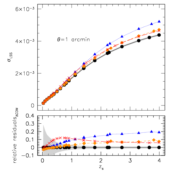
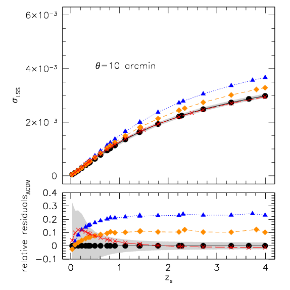
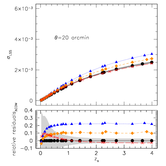
In Fig. 14 we show, for the four considered cosmologies, the noise produced by the LSS on spherically averaged shear profiles. The results are presented for three typical scales ($\theta$=1, 10 and 20 arcmin) and considering sources up to redshift $z_{s}=4$. As already done in the case of the aperture mass statistics, the results are directly extracted from the convergence maps that have been smoothed using the appropriate $J_{2}$ kernel.

From the figure we notice that the noise produced by large scale structures is higher in the cDE models with respect to the $\mathrm{\Lambda}$CDM cosmology. This is particularly true for the EXP003 and EXP008e3 models: for $\theta>10$ arcmin and for sources with $z_{s}>0.5$ they present values that are about 20 and 10 percent larger than the one measured in the $\mathrm{\Lambda}$CDM model, respectively. For the SUGRA003 model, a smaller increase of noise is evident only for $\theta=1$ arcmin and/or for sources at low redshift. We underline also that the rms of the measurement $\mathrm{\Lambda}$CDM decreases as a function of redshifts because of a combination of ($i$) the choice filter, ($ii$) the field of view and ($iii$) the clustering of the haloes as a function of redshifts – at high redshift the universe is more homogenius.

References

- Amara et al. (2012) Amara A., Lilly S., Kovač K., Rhodes J., Massey R., Zamorani G., Carollo et al. 2012, MNRAS, 424, 553
- Bahé et al. (2012) Bahé Y. M., McCarthy I. G., King L. J., 2012, MNRAS, 421, 1073
- Baldi (2012a) Baldi M., 2012a, MNRAS, 420, 430
- Baldi (2012b) Baldi M., 2012b, MNRAS, 420, 430
- Baldi (2012c) Baldi M., 2012c, MNRAS, 422, 1028
- Baldi et al. (2011) Baldi M., Lee J., Macciò A. V., 2011, ApJ, 732, 112
- Baldi et al. (2011) Baldi M., Pettorino V., Amendola L., Wetterich C., 2011, MNRAS, 418, 214
- Baldi et al. (2010) Baldi M., Pettorino V., Robbers G., Springel V., 2010, MNRAS, 403, 1684
- Baldi & Viel (2010) Baldi M., Viel M., 2010, MNRAS, 409, L89
- Bartelmann (1996) Bartelmann M., 1996, A&A, 313, 697
- Bartelmann (2010) Bartelmann M., 2010, ArXiv e-prints
- Bartelmann & Schneider (2001) Bartelmann M., Schneider P., 2001, Physics Reports, 340, 291
- Becker (2013) Becker M. R., 2013, MNRAS, 435, 115
- Bellagamba et al. (2011) Bellagamba F., Maturi M., Hamana T., Meneghetti M., Miyazaki S., Moscardini L., 2011, MNRAS, 413, 1145
- Benjamin et al. (2013) Benjamin J., Van Waerbeke L., Heymans C., Kilbinger M., Erben T., Hildebrandt H., Hoekstra H., et al. 2013, MNRAS, 431, 1547
- Bernstein & Jarvis (2002) Bernstein G. M., Jarvis M., 2002, AJ, 123, 583
- Beynon et al. (2012) Beynon E., Baldi M., Bacon D. J., Koyama K., Sabiu C., 2012, MNRAS, 422, 3546
- Boldrin et al. (2012) Boldrin M., Giocoli C., Meneghetti M., Moscardini L., 2012, MNRAS, 427, 3134
- Brax & Martin (1999) Brax P. H., Martin J., 1999, Physics Letters B, 468, 40
- Bridle et al. (2010) Bridle S., Balan S. T., Bethge M., Gentile M., Harmeling S., Heymans C., Hirsch M., et al. 2010, MNRAS, 405, 2044
- Carbone et al. (2013) Carbone C., Baldi M., Pettorino V., Baccigalupi C., 2013, JCAP, 9, 4
- Cui et al. (2012) Cui W., Baldi M., Borgani S., 2012, MNRAS, 424, 993
- Fedeli et al. (2014) Fedeli C., Semboloni E., Velliscig M., Van Daalen M., Schaye J., Hoekstra H., 2014, JCAP, 8, 28
- Fu et al. (2008) Fu L., Semboloni E., Hoekstra H., Kilbinger M., van Waerbeke L., Tereno I., Mellier Y., Heymans C., Coupon J., Benabed K., Benjamin J., Bertin E., Doré O., Hudson M. J., Ilbert O., Maoli et al. 2008, A&A, 479, 9
- Giocoli et al. (2013) Giocoli C., Marulli F., Baldi M., Moscardini L., Metcalf R. B., 2013, MNRAS, 434, 2982
- Giocoli et al. (2012a) Giocoli C., Meneghetti M., Bartelmann M., Moscardini L., Boldrin M., 2012a, MNRAS, 421, 3343
- Giocoli et al. (2014) Giocoli C., Meneghetti M., Metcalf R. B., Ettori S., Moscardini L., 2014, MNRAS, 440, 1899
- Giocoli et al. (2007) Giocoli C., Moreno J., Sheth R. K., Tormen G., 2007, MNRAS, 376, 977
- Harnois-Déraps et al. (2012) Harnois-Déraps J., Vafaei S., Van Waerbeke L., 2012, MNRAS, 426, 1262
- Harnois-Déraps et al. (2014) Harnois-Déraps J., van Waerbeke L., Viola M., Heymans C., 2014, ArXiv e-prints
- Heymans et al. (2013) Heymans C., Grocutt E., Heavens A., Kilbinger M., Kitching T. D., Simpson F., Benjamin J., Erben T., et al. 2013, MNRAS, 432, 2433
- Heymans et al. (2012) Heymans C., Rowe B., Hoekstra H., Miller L., Erben T., Kitching T., van Waerbeke L., 2012, MNRAS, 421, 381
- Hilbert et al. (2008) Hilbert S., White S. D. M., Hartlap J., Schneider P., 2008, MNRAS, 386, 1845
- Hildebrandt et al. (2012) Hildebrandt H., Erben T., Kuijken K., van Waerbeke L., Heymans C., Coupon J., Benjamin J., et al. 2012, MNRAS, 421, 2355
- Hockney & Eastwood (1988) Hockney R. W., Eastwood J. W., 1988, Computer simulation using particles
- Hoekstra (2003) Hoekstra H., 2003, MNRAS, 339, 1155
- Hoekstra et al. (2011) Hoekstra H., Hartlap J., Hilbert S., van Uitert E., 2011, MNRAS, 412, 2095
- Hoekstra et al. (2012) Hoekstra H., Mahdavi A., Babul A., Bildfell C., 2012, MNRAS, 427, 1298
- Jullo et al. (2007) Jullo E., Kneib J.-P., Limousin M., Elíasdóttir Á., Marshall P. J., Verdugo T., 2007, New Journal of Physics, 9, 447
- Kacprzak et al. (2012) Kacprzak T., Zuntz J., Rowe B., Bridle S., Refregier A., Amara A., et al. 2012, MNRAS, 427, 2711
- Kaiser (1992) Kaiser N., 1992, Astrophys. J., 388, 272
- Kaiser & Squires (1993) Kaiser N., Squires G., 1993, ApJ, 404, 441
- Kaiser et al. (1995) Kaiser N., Squires G., Broadhurst T., 1995, ApJ, 449, 460
- Kilbinger (2014) Kilbinger M., 2014, ArXiv e-prints
- Kilbinger et al. (2013) Kilbinger M., Fu L., Heymans C., Simpson F., Benjamin J., Erben T., Harnois-Déraps J., Hoekstra H., Hildebrandt H., et al. 2013, MNRAS, 430, 2200
- Kitching et al. (2014) Kitching T. D., Heavens A. F., Alsing J., Erben T., Heymans C., Hildebrandt H., Hoekstra H., et al. 2014, MNRAS, 442, 1326
- Kitching et al. (2014b) Kitching T. D., Heavens A. F., Das S., 2014b, ArXiv e-prints
- Kneib & Natarajan (2011) Kneib J.-P., Natarajan P., 2011, A&A Rev., 19, 47
- Komatsu et al. (2011) Komatsu E., Smith K. M., Dunkley J., Bennett C. L., Gold B., Hinshaw G., Jarosik N., Larson D., Nolta M. R., et al. 2011, ApJS, 192, 18
- Kowalski et al. (2008) Kowalski M., Rubin D., Aldering G., Agostinho R. J., Amadon A., Amanullah R., Balland C., Barbary K., Blanc et al. 2008, ApJ, 686, 749
- Lacey & Cole (1993) Lacey C., Cole S., 1993, MNRAS, 262, 627
- Laureijs et al. (2011) Laureijs R., Amiaux J., Arduini S., Auguères J. ., Brinchmann J., Cole R., Cropper M., Dabin C., Duvet L., et al. 2011, ArXiv e-prints
- Lewis et al. (2000) Lewis A., Challinor A., Lasenby A., 2000, Astrophys. J., 538, 473
- Lucchin & Matarrese (1985) Lucchin F., Matarrese S., 1985, Phys.Rev.D, 32, 1316
- Mandelbaum et al. (2006b) Mandelbaum R., Seljak U., Cool R. J., Blanton M., Hirata C. M., Brinkmann J., 2006b, MNRAS, 372, 758
- Marulli et al. (2012) Marulli F., Baldi M., Moscardini L., 2012, MNRAS, 420, 2377
- Maturi et al. (2005) Maturi M., Meneghetti M., Bartelmann M., Dolag K., Moscardini L., 2005, A&A, 442, 851
- Meneghetti et al. (2005a) Meneghetti M., Bartelmann M., Dolag K., Moscardini L., Perrotta F., Baccigalupi C., Tormen G., 2005a, A&A, 442, 413
- Meneghetti et al. (2008) Meneghetti M., Melchior P., Grazian A., De Lucia G., Dolag K., Bartelmann M., Heymans C., Moscardini L., Radovich M., 2008, A&A, 482, 403
- Merten et al. (2009) Merten J., Cacciato M., Meneghetti M., Mignone C., Bartelmann M., 2009, A&A, 500, 681
- Merten et al. (2014) Merten J., Meneghetti M., Postman M., Umetsu K., Zitrin A., Medezinski E., Nonino M., Koekemoer A., Melchior P., Gruen D., et al. 2014, ArXiv e-prints
- Metcalf & Petkova (2013) Metcalf R. B., Petkova M., 2013, ArXiv e-prints
- Miller et al. (2013) Miller L., Heymans C., Kitching T. D., van Waerbeke L., Erben T., Hildebrandt H., Hoekstra H., et al. 2013, MNRAS, 429, 2858
- Moresco et al. (2014) Moresco M., Marulli F., Baldi M., Moscardini L., Cimatti A., 2014, MNRAS, 443, 2874
- Navarro et al. (1996) Navarro J. F., Frenk C. S., White S. D. M., 1996, ApJ, 462, 563
- Navarro et al. (2004) Navarro J. F., Hayashi E., Power C., Jenkins A. R., Frenk C. S., White S. D. M., Springel V., Stadel J., Quinn T. R., 2004, MNRAS, 349, 1039
- Oguri et al. (2012) Oguri M., Bayliss M. B., Dahle H., Sharon K., Gladders M. D., Natarajan P., Hennawi J. F., Koester B. P., 2012, MNRAS, 420, 3213
- Okabe et al. (2010b) Okabe N., Takada M., Umetsu K., Futamase T., Smith G. P., 2010b, PASJ, 62, 811
- Pace et al. (2015) Pace F., Baldi M., Moscardini L., Bacon D., Crittenden R., 2015, MNRAS, 447, 858
- Perlmutter et al. (1999) Perlmutter S., et al., 1999, Astrophys. J., 517, 565
- Petkova et al. (2013) Petkova M., Metcalf R. B., Giocoli C., 2013, ArXiv e-prints
- Planck Collaboration et al. (2013) Planck Collaboration Ade P. A. R., Aghanim N., Armitage-Caplan C., Arnaud M., Ashdown M., Atrio-Barandela F., Aumont J., Baccigalupi C., Banday A. J., et al. 2013, ArXiv e-prints
- Refregier et al. (2004) Refregier A., Massey R., Rhodes J., Ellis R., Albert J., Bacon D., Bernstein G., McKay T., Perlmutter S., 2004, AJ, 127, 3102
- Refregier et al. (2002) Refregier A., Rhodes J., Groth E. J., 2002, ApJ, 572, L131
- Riess et al. (1998) Riess A. G., et al., 1998, Astron. J., 116, 1009
- Roncarelli et al. (2007) Roncarelli M., Moscardini L., Borgani S., Dolag K., 2007, MNRAS, 378, 1259
- Sato et al. (2009) Sato M., Hamana T., Takahashi R., Takada M., Yoshida N., Matsubara T., Sugiyama N., 2009, ApJ, 701, 945
- Sato & Nishimichi (2013) Sato M., Nishimichi T., 2013, Phys.Rev.D, 87, 123538
- Schmidt et al. (1998) Schmidt B. P., et al., 1998, Astrophys.J., 507, 46
- Schneider et al. (1998) Schneider P., van Waerbeke L., Jain B., Kruse G., 1998, MNRAS, 296, 873
- Schrabback et al. (2010) Schrabback T., Hartlap J., Joachimi B., Kilbinger M., Simon P., Benabed K., Bradač M., Eifler T., Erben et al. 2010, A&A, 516, A63+
- Semboloni et al. (2013) Semboloni E., Hoekstra H., Schaye J., 2013, MNRAS, 434, 148
- Sereno et al. (2014) Sereno M., Giocoli C., Ettori S., Moscardini L., 2014, ArXiv e-prints
- Smith et al. (2003) Smith R. E., Peacock J. A., Jenkins A., White S. D. M., Frenk C. S., Pearce F. R., Thomas P. A., Efstathiou G., Couchman H. M. P., 2003, MNRAS, 341, 1311
- Springel (2005) Springel V., 2005, MNRAS, 364, 1105
- Springel et al. (2005) Springel V., White S. D. M., Jenkins A., Frenk C. S., Yoshida N., Gao L., Navarro J., Thacker R., Croton D., Helly J., Peacock J. A., Cole S., Thomas P., Couchman H., Evrard A., Colberg J., Pearce F., 2005, Nature, 435, 629
- Suzuki et al. (2012) Suzuki N., Rubin D., Lidman C., Aldering G., Amanullah R., Barbary K., Barrientos L. F., Botyanszki J., Brodwin M., Connolly e. a., 2012, ApJ, 746, 85
- Takahashi et al. (2011) Takahashi R., Oguri M., Sato M., Hamana T., 2011, ApJ, 742, 15
- Takahashi et al. (2012) Takahashi R., Sato M., Nishimichi T., Taruya A., Oguri M., 2012, ApJ, 761, 152
- Tormen (1998) Tormen G., 1998, MNRAS, 297, 648
- van Waerbeke (2000) van Waerbeke L., 2000, MNRAS, 313, 524
- von der Linden et al. (2014) von der Linden A., Allen M. T., Applegate D. E., Kelly P. L., Allen S. W., Ebeling H., Burchat P. R., Burke D. L., Donovan D., Morris R. G., Blandford R., Erben T., Mantz A., 2014, MNRAS, 439, 2
- von der Linden et al. (2014b) von der Linden A., Mantz A., Allen S. W., Applegate D. E., Kelly P. L., Morris R. G., Wright A., Allen M. T., Burchat P. R., Burke D. L., Donovan D., Ebeling H., 2014b, MNRAS, 443, 1973
- Wetterich (1988) Wetterich C., 1988, Nuclear Physics B, 302, 668
- Zitrin et al. (2011) Zitrin A., Broadhurst T., Barkana R., Rephaeli Y., Benítez N., 2011, MNRAS, 410, 1939