Fast Embedding for JOFC Using the Raw Stress Criterion

Vince Lyzinski  
Johns Hopkins University Human Language Technology Center of Excellence,
Youngser Park
Center for Imaging Sciences, Johns Hopkins University,
Carey E. Priebe
Department of Applied Mathematics and Statistics, Johns Hopkins University,
and
Michael Trosset
Department of Statistics, Indiana University
The authors gratefully acknowledge support from the XDATA program of the Defense Advanced Research Projects Agency (DARPA) administered through Air Force Research Laboratory contract FA8750-12-2-0303, and the NSF BRAIN Early Concept Grants for Exploratory Research (EAGER) award DBI-1451081.
Abstract

The Joint Optimization of Fidelity and Commensurability (JOFC) manifold matching methodology embeds an omnibus dissimilarity matrix consisting of multiple dissimilarities on the same set of objects. One approach to this embedding optimizes the preservation of fidelity to each individual dissimilarity matrix together with commensurability of each given observation across modalities via iterative majorization of a raw stress error criterion by successive Guttman transforms. In this paper, we exploit the special structure inherent to JOFC to exactly and efficiently compute the successive Guttman transforms, and as a result we are able to greatly speed up the JOFC procedure for both in-sample and out-of-sample embedding. We demonstrate the scalability of our implementation on both real and simulated data examples.


Keywords: Multidimensional Scaling, manifold matching, distance geometry, distance matrices

1 Introduction and Background

Manifold matching—embedding multiple modality data sets into a common low-dimensional space wherein joint inference can be investigated—is an important inference task in statistical pattern recognition, with applications in computer vision (see, for example, Nastar et al., 1996; Hardoon et al., 2004; Elgammal and Lee, 2004; Wang and Suter, 2007; Ham et al., 2003), text and language processing (see, for example, Karakos et al., 2007; Vinokourov et al., 2002; Sahami and Heilman, 2006), and machine learning (see, for example, Wang and Mahadevan, 2008, 2009; Lafon et al., 2006; Ham et al., 2005), to name a few; for a survey of the literature on manifold matching and the broader problem of transfer learning, see Pan and Yang (2010).

In the present manifold matching framework, we consider n𝑛n objects, each measured under m𝑚m disparate modalities or conditions, each modality yielding an object-wise dissimilarity matrix {Δi}i=1msuperscriptsubscriptsubscriptΔ𝑖𝑖1𝑚\{\Delta_{i}\}_{i=1}^{m}; thus Δ1,Δ2,,Δm+n×nsubscriptΔ1subscriptΔ2subscriptΔ𝑚superscriptsubscript𝑛𝑛\Delta_{1},\Delta_{2},\ldots,\Delta_{m}\in\mathbb{R}_{+}^{n\times n}. The Joint Optimization of Fidelity and Commensurability (JOFC) algorithm of Priebe et al. (2013) is a manifold matching procedure that simultaneously embeds these mn𝑚𝑛mn data points (n𝑛n objects in m𝑚m modalities) into a common Euclidean space by embedding an omnibus dissimilarity matrix 𝚫𝚫{\bf\Delta} which encapsulates the information contained in the dissimilarities {Δi}i=1msuperscriptsubscriptsubscriptΔ𝑖𝑖1𝑚\{\Delta_{i}\}_{i=1}^{m}. The JOFC algorithm has proven to be a flexible and effective manifold matching algorithm, with numerous applications and extensions in the literature; see Ma et al. (2012); Sun and Priebe (2013); Lyzinski et al. (2013); Adali and Priebe (2015); Shen et al. (2016). One approach to this embedding optimizes the preservation of fidelity to each individual dissimilarity matrix (i.e., preserving the within modality dissimilarities) together with the commensurability of the observations across modalities (i.e., preserving the cross-modality matchedness of the data). This approach embeds 𝚫𝚫{\bf\Delta} by minimizing Kruskal’s raw stress criterion for metric multidimensional scaling (MDS) via successive Guttman transforms (Borg and Groenen, 2005); see Algorithm 1.

In this paper, we exploit the special structure of the JOFC weight matrix to exactly and efficiently compute these successive Guttman transforms. Employing this and further computational simplifications, we are able to dramatically speed the JOFC procedure (see Algorithm 2) and extend this speedup to out-of-sample embedding for JOFC. In addition, parallelizing the resulting algorithm—see Remark 8—is immediate. We demonstrate these speedups and the utility of the JOFC framework in real and synthetic data examples.

Notation: To aid the reader, we have collected the frequently used notation introduced in this manuscript into a table for ease of reference; see Table 1.

Notation Description Reference
Jnsubscript𝐽𝑛J_{n} The n×n𝑛𝑛n\times n matrix of all 111’s Used throughout
Insubscript𝐼𝑛I_{n} The n×n𝑛𝑛n\times n identity matrix Used throughout
X Final configuration obtained via 3-RSMDS JOFC and fJOFC Sec. 1.2, 1.2.1 and 2
σ~(𝐗)~𝜎𝐗\tilde{\sigma}(\bf X) The raw stress objective fcn. of 3-RSMDS Eq. (1)
𝚫~~𝚫\widetilde{\bf\Delta} The omnibus dissimilarity embedded by 3-RSMDS Eq. (2)
σ(𝐗)𝜎𝐗\sigma(\bf X) The raw stress objective fcn. of JOFC and fJOFC Eq. (3)
𝚫𝚫{\bf\Delta} The omnibus dissimilarity embedded by JOFC and fJOFC Eq. (5)
𝐖𝐖\bf W The weight matrix used in the JOFC and fJOFC embeddings Eq. (6)
𝐋𝐋\bf L The combinatorial Laplacian of 𝐖𝐖\bf W Sec. 1.2.1 and 2
B(𝐗)𝐵𝐗B({\bf X}) The B𝐵B-matrix used in the JOFC Guttman transform updates Eq. (7)
𝐋superscript𝐋\bf L^{\dagger} The Moore-Penrose pseudoinverse of 𝐋𝐋\bf L Sec. 1.2.1 and 2
𝒲𝒲\mathcal{W} A modified weight matrix used in the computation of 𝐋superscript𝐋\bf L^{\dagger} Eq. (10)
𝚫(o)superscript𝚫𝑜{\bf\Delta}^{(o)} The out-of-sample omnibus dissimilarity embedded by fJOFC Sec. 3
σ𝐗(𝐲)subscript𝜎𝐗𝐲\sigma_{\bf X}({\bf y}) The out-of-sample raw stress criterion Sec. 3
𝐖(o)superscript𝐖𝑜{\bf W}^{(o)} The out-of-sample weight matrix used in the fJOFC embedding Sec. 3
𝐋(o)superscript𝐋𝑜{\bf L}^{(o)} The combinatorial Laplacian of 𝐖(o)superscript𝐖𝑜{\bf W}^{(o)} Sec. 3
Table 1: Table of relevant notation.

1.1 JOFC and Three-Way Raw Stress MDS

In the JOFC framework, we use Raw Stress MDS to simultaneously embed the m𝑚m object-wise dissimilarity matrices Δ1,Δ2,,Δm+n×nsubscriptΔ1subscriptΔ2subscriptΔ𝑚subscriptsuperscript𝑛𝑛\Delta_{1},\Delta_{2},\ldots,\Delta_{m}\in\mathbb{R}^{n\times n}_{+} while preserving both the matchedness of the objects across modality and the within modality dissimilarities. In this way, JOFC is closely related to Three-Way Raw Stress MDS (3-RSMDS). The key difference is that the cross modality matchedness of the objects in 3-RSMDS is enforced via a constraint on the feasible region, while in JOFC the matchedness is enforced by adding a suitable term into the raw stress criterion. In that light, JOFC can be viewed as a softly constrained version of 3-RSMDS. We highlight the commonalities and differences between the two approaches below, and in Section 4.1 empirically compare their respective performances in an illustrative simulation. For further discussion of the connection between JOFC and Three-Way Nonmetric MDS in the context of hypothesis testing, see Castle (2012), Chapter 8.

Remark 1.

While the JOFC algorithm is closely related to 3-RSMDS, it bears mentioning the relationship of the algorithm to other existing manifold alignment procedures. Many existing algorithms begin with a set of high-dimensional points sampled or observed from manifolds in ksuperscript𝑘\mathbb{R}^{k}; see, for example, Ham et al. (2005); Wang and Suter (2007); Sharma et al. (2012). Dimension reduction techniques are then applied jointly to the observations to align the manifolds in a common d𝑑d-dimensional embedding space with dkmuch-less-than𝑑𝑘d\ll k. In JOFC—similar to many of MDS and kernel based methods; see, for example, Leeuw and Mair (2008); Wang and Mahadevan (2008); Shen et al. (2016)—often the objects’ measurements cannot be made in Euclidean space. For example, the views of a single object may represent the i. text content, ii. images, iii. communication activity associated with a single social media profile. While these data are non-Euclidean by nature, nonetheless there are well established dissimilarities that can be computed within each modality. Indeed, the only requirement in the JOFC framework is that we can compute dissimilarities amongst the data points within each modality.

1.2 Three-Way Raw Stress MDS

In both the 3-RSMDS and the JOFC frameworks, we seek to simultaneously embed the m𝑚m object-wise dissimilarity matrices, and in both regimes, the m𝑚m dissimilarities are measured between the same n𝑛n objects; i.e., they are produced by repeated measurements or observations under potentially disparate modalities. Assuming that the entire cross-modality correspondence is known a priori between the n𝑛n objects, Three-Way Raw Stress Multidimensional Scaling (3-RSMDS) seeks to find a configuration

𝐗=[(𝐗(1))|(𝐗(2))||(𝐗(m))]mn×d,superscript𝐗topdelimited-[]conditionalsuperscriptsuperscript𝐗1topsuperscriptsuperscript𝐗2topsuperscriptsuperscript𝐗𝑚topsuperscript𝑚𝑛𝑑{\bf X}^{\top}=\left[({\bf X}^{(1)})^{\top}|({\bf X}^{(2)})^{\top}|\cdots|({\bf X}^{(m)})^{\top}\right]\in\mathbb{R}^{mn\times d},

of the mn𝑚𝑛mn points that minimizes the raw stress criterion,

σ~(𝐗)=i=1mj<k([Δi]j,kdj,k(𝐗(i)))2,~𝜎𝐗superscriptsubscript𝑖1𝑚subscript𝑗𝑘superscriptsubscriptdelimited-[]subscriptΔ𝑖𝑗𝑘subscript𝑑𝑗𝑘superscript𝐗𝑖2\tilde{\sigma}({\bf X})=\sum_{i=1}^{m}\sum_{j<k}\left([\Delta_{i}]_{j,k}-d_{j,k}({\bf X}^{(i)})\right)^{2}, (1)

subject to the constraint that 𝐗(i)=𝐆𝐖(i)superscript𝐗𝑖superscript𝐆𝐖𝑖{\bf X}^{(i)}={\bf GW}^{(i)} for all i[m]:={1,2,,m}𝑖delimited-[]𝑚assign12𝑚i\in[m]:=\{1,2,\ldots,m\} (note that to remove nonidentifiability issues, 𝐆𝐆{\bf G} is often constrained to satisfy 𝐆𝐆=Insuperscript𝐆𝐆topsubscript𝐼𝑛{\bf G}{\bf G}^{\top}=I_{n}). In (1), for 𝐌k×𝐌superscript𝑘{\bf M}\in\mathbb{R}^{k\times\ell}, di,j(𝐌)subscript𝑑𝑖𝑗𝐌d_{i,j}({\bf M}) is the Euclidean distance between the i𝑖i-th and j𝑗j-th rows of 𝐌𝐌{\bf M}, and for i[n]𝑖delimited-[]𝑛i\in[n], 𝐗(i)superscript𝐗𝑖{\bf X}^{(i)} are the embedded points in dsuperscript𝑑\mathbb{R}^{d} corresponding to ΔisubscriptΔ𝑖\Delta_{i}. Adopting the terminology in Borg and Groenen (2005), in the dimension-weighting 3-RSMDS model, 𝐆𝐆{\bf G} is known as the group stimulus space, and the 𝐖(i)superscript𝐖𝑖{\bf W}^{(i)} are diagonal matrices with nonnegative diagonal entries. In this model, the individual embeddings 𝐗(i)superscript𝐗𝑖{\bf X}^{(i)} differ only in the (potentially different) weights— given by the diagonal entries of the respective 𝐖(i)superscript𝐖𝑖{\bf W}^{(i)}’s—they place on the dimensions of 𝐆𝐆{\bf G}.

The 3-RSMDS dimension weighting model and its variants have been well-studied in the literature; see, for example, Carroll and Chang (1970); Carroll and Wish (1974); Schulz (1980); De Leeuw and Heiser (1980); Heiser (1988); Harshman and Lundy (1984). Indeed, there are a number of proposed procedures in the literature for solving the Three-Way MDS problem under a variety of error criterion, including the INDSCAL algorithm of Carroll and Chang (1970); the IDIOSCAL algorithm of Carroll and Wish (1974); Schulz (1980); the PROXSCAL algorithm of Heiser (1988); and the PARAFAC algorithm of Harshman and Lundy (1984); among numerous others. We note here that minimizing (1) subject to the constraint 𝐗(i)=𝐆𝐖(i)superscript𝐗𝑖superscript𝐆𝐖𝑖{\bf X}^{(i)}={\bf GW}^{(i)} for all i{1,2,,m}𝑖12𝑚i\in\{1,2,\ldots,m\} is equivalent to performing constrained Raw Stress MDS on the dissimilarity matrix

𝚫~=[Δ1NANANAΔ2NANANAΔm]mn×mn~𝚫matrixsubscriptΔ1NANANAsubscriptΔ2NANANAsubscriptΔ𝑚superscript𝑚𝑛𝑚𝑛\widetilde{\bf\Delta}=\begin{bmatrix}\Delta_{1}&\text{NA}&\cdots&\text{NA}\\ \text{NA}&\Delta_{2}&\cdots&\text{NA}\\ \vdots&\vdots&\ddots&\vdots\\ \text{NA}&\text{NA}&\cdots&\Delta_{m}\end{bmatrix}\in\mathbb{R}^{mn\times mn} (2)

with configuration matrix

𝐗=[(𝐗(1))|(𝐗(2))||(𝐗(m))]mn×d,superscript𝐗topdelimited-[]conditionalsuperscriptsuperscript𝐗1topsuperscriptsuperscript𝐗2topsuperscriptsuperscript𝐗𝑚topsuperscript𝑚𝑛𝑑{\bf X}^{\top}=\left[({\bf X}^{(1)})^{\top}|({\bf X}^{(2)})^{\top}|\cdots|({\bf X}^{(m)})^{\top}\right]\in\mathbb{R}^{mn\times d},

subject to 𝐗(i)=𝐆𝐖(i)superscript𝐗𝑖superscript𝐆𝐖𝑖{\bf X}^{(i)}={\bf GW}^{(i)} for all i[m]𝑖delimited-[]𝑚i\in[m]. The “NA” entries in 𝚫𝚫{\bf\Delta} represent the reality that the dissimilarities across modalities are unknown a priori. This is accounted for in the objective function by zeroing out the contribution to the stress associated with these entries of 𝚫~~𝚫\widetilde{\bf\Delta}. the weight matrix 𝐖𝐖\bf W is structured to zero out the missing data entries of η𝜂\eta in the objective function σ().𝜎\sigma(\cdot).. The constrained MDS iterative majorization algorithm of De Leeuw and Heiser (1980) can then be applied to approximately solve the 3-RSMDS model. As the JOFC procedure (see Algorithm 1) and the accelerated fJOFC procedure (see Algorithm 2) are both iterative majorization MDS procedures, we will provide the details of De Leeuw and Heiser (1980) applied to 3-RSMDS for the sake of comparison. The procedure of De Leeuw and Heiser (1980) consists of the following two iterated steps, given an initialization of the configuration 𝐗(0)subscript𝐗0{\bf X}_{(0)}:

  • 1.

    At configuration 𝐗(t1)subscript𝐗𝑡1{\bf X}_{(t-1)}, ignoring the constraint that 𝐗(i)=𝐆𝐖(i)superscript𝐗𝑖superscript𝐆𝐖𝑖{\bf X}^{(i)}={\bf GW}^{(i)} for all i[m]𝑖delimited-[]𝑚i\in[m], compute the unconstrained update 𝐗~(t)subscript~𝐗𝑡\widetilde{\bf X}_{(t)} via the Guttman transform; see Borg and Groenen (2005).

  • 2.

    Set 𝐗(t)=[(𝐗(t)(1))|(𝐗(t)(2))||(𝐗(t)(m))]subscript𝐗𝑡delimited-[]conditionalsuperscriptsubscriptsuperscript𝐗1𝑡topsuperscriptsubscriptsuperscript𝐗2𝑡topsuperscriptsubscriptsuperscript𝐗𝑚𝑡top{\bf X}_{(t)}=\left[\big{(}{\bf X}^{(1)}_{(t)}\big{)}^{\top}|\big{(}{\bf X}^{(2)}_{(t)}\big{)}^{\top}|\cdots|\big{(}{\bf X}^{(m)}_{(t)}\big{)}^{\top}\right] to be the minimizer of

    trace(𝐗𝐗~(t))𝐋~(𝐗𝐗~(t)),tracesuperscript𝐗subscript~𝐗𝑡top~𝐋𝐗subscript~𝐗𝑡\textup{trace}({\bf X}-\widetilde{\bf X}_{(t)})^{\top}\widetilde{\bf L}({\bf X}-\widetilde{\bf X}_{(t)}),

    over 𝐗𝐗{\bf X} subject to the constraints 𝐗(i)=𝐆𝐖(i)superscript𝐗𝑖superscript𝐆𝐖𝑖{\bf X}^{(i)}={\bf GW}^{(i)} for all i{1,2,,m}𝑖12𝑚i\in\{1,2,\ldots,m\}. Here, 𝐋~mn×mn~𝐋superscript𝑚𝑛𝑚𝑛\widetilde{\bf L}\in\mathbb{R}^{mn\times mn} is the block diagonal matrix with nInJnn×n𝑛subscript𝐼𝑛subscript𝐽𝑛superscript𝑛𝑛nI_{n}-J_{n}\in\mathbb{R}^{n\times n} in each of the m𝑚m diagonal blocks, where Jn=𝟏n𝟏nTn×nsubscript𝐽𝑛subscript1𝑛superscriptsubscript1𝑛𝑇superscript𝑛𝑛J_{n}={\bf 1}_{n}{\bf 1}_{n}^{T}\in\mathbb{R}^{n\times n}, and 𝟏nsubscript1𝑛{\bf 1}_{n} is the column vector of all one’s in nsuperscript𝑛\mathbb{R}^{n}. This minimization is often approached by alternating minimizing over 𝐆𝐆{\bf G} for a fixed 𝐖𝐖{\bf W} and then minimizing over 𝐖𝐖{\bf W} for a fixed 𝐆𝐆{\bf G}.

1.2.1 The JOFC framework

In the above 3-RSMDS framework, the matchedness of the n𝑛n observations across the m𝑚m dissimilarities is enforced via the 𝐗(i)=𝐆𝐖(i)superscript𝐗𝑖superscript𝐆𝐖𝑖{\bf X}^{(i)}={\bf GW}^{(i)} constraints. In the JOFC algorithm, the matchedness constraint is built into the objective function as follows. Contrasting the raw stress criterion in (1), the variant of JOFC we consider seeks to produce an unconstrained configuration 𝐗=[(𝐗(1))|(𝐗(2))||(𝐗(m))]mn×d,superscript𝐗topdelimited-[]conditionalsuperscriptsuperscript𝐗1topsuperscriptsuperscript𝐗2topsuperscriptsuperscript𝐗𝑚topsuperscript𝑚𝑛𝑑{\bf X}^{\top}=\left[({\bf X}^{(1)})^{\top}|({\bf X}^{(2)})^{\top}|\cdots|({\bf X}^{(m)})^{\top}\right]\in\mathbb{R}^{mn\times d}, (where (𝐗(i))=[(X1(i))|(X2(i))||(Xm(i))]n×d,superscriptsuperscript𝐗𝑖topdelimited-[]conditionalsuperscriptsubscriptsuperscript𝑋𝑖1topsuperscriptsubscriptsuperscript𝑋𝑖2topsuperscriptsuperscriptsubscript𝑋𝑚𝑖topsuperscript𝑛𝑑({\bf X}^{(i)})^{\top}=\left[({X}^{(i)}_{1})^{\top}|({X}^{(i)}_{2})^{\top}|\cdots|({X}_{m}^{(i)})^{\top}\right]\in\mathbb{R}^{n\times d}, are the points associated with ΔisubscriptΔ𝑖\Delta_{i}) that minimizes the raw stress criterion

σ(𝐗)=i=1m1j<n([Δi]j,dj,(𝐗(i)))2fidelity+w1i<jm=1nd(X(i),X(j))2commensurability,𝜎𝐗subscriptsuperscriptsubscript𝑖1𝑚subscript1𝑗𝑛superscriptsubscriptdelimited-[]subscriptΔ𝑖𝑗subscript𝑑𝑗superscript𝐗𝑖2fidelity𝑤subscriptsubscript1𝑖𝑗𝑚superscriptsubscript1𝑛𝑑superscriptsubscriptsuperscript𝑋𝑖subscriptsuperscript𝑋𝑗2commensurability\displaystyle\sigma({\bf X})=\underbrace{\sum_{i=1}^{m}\sum_{1\leq j<\,\ell\leq n}\left([\Delta_{i}]_{j,\ell}-d_{j,\ell}({\bf X}^{(i)})\right)^{2}}_{\text{fidelity}}+w\underbrace{\sum_{1\leq i<j\leq m}\sum_{\ell=1}^{n}d(X^{(i)}_{\ell},X^{(j)}_{\ell})^{2}}_{\text{commensurability}}, (3)

where d(,)𝑑d(\cdot,\cdot) is the Euclidean distance function. The raw stress criterion in JOFC is composed of three major pieces:

  • 1.

    The “fidelity” term, i=1m1j<n([Δi]j,dj,(𝐗(i)))2superscriptsubscript𝑖1𝑚subscript1𝑗𝑛superscriptsubscriptdelimited-[]subscriptΔ𝑖𝑗subscript𝑑𝑗superscript𝐗𝑖2\sum_{i=1}^{m}\sum_{1\leq j<\,\ell\leq n}\left([\Delta_{i}]_{j,\ell}-d_{j,\ell}({\bf X}^{(i)})\right)^{2}, which measures the faithfulness of the embedding to the original dissimilarities, {Δi}i=1msuperscriptsubscriptsubscriptΔ𝑖𝑖1𝑚\{\Delta_{i}\}_{i=1}^{m}. Note the the fidelity is equal to the raw stress criterion in 3-RSMDS (1).

  • 2.

    The “commensurability” term, 1i<jm=1nd(X(i),X(j))2subscript1𝑖𝑗𝑚superscriptsubscript1𝑛𝑑superscriptsubscriptsuperscript𝑋𝑖subscriptsuperscript𝑋𝑗2\sum_{1\leq i<j\leq m}\sum_{\ell=1}^{n}d(X^{(i)}_{\ell},X^{(j)}_{\ell})^{2}, which measures how the geometry of the embeddings differs across modality. Similar to the role of the 𝐗(i)=𝐆𝐖(i)superscript𝐗𝑖superscript𝐆𝐖𝑖{\bf X}^{(i)}={\bf GW}^{(i)} constraints in 3-RSMDS, in JOFC the commensurability term (softly) enforces the matchedness of the n𝑛n data points across the m𝑚m modalities. We also note that the commensurability is proportional to the objective function of three-way Procrustes analysis

    commensurability =i<jmtrace(𝐗(i)𝐗(j))(𝐗(i)𝐗(j))absentsuperscriptsubscript𝑖𝑗𝑚tracesuperscriptsuperscript𝐗𝑖superscript𝐗𝑗topsuperscript𝐗𝑖superscript𝐗𝑗\displaystyle=\sum_{i<j}^{m}\textup{trace}({\bf X}^{(i)}-{\bf X}^{(j)})^{\top}({\bf X}^{(i)}-{\bf X}^{(j)})
    =mi=1mtrace(𝐗(i)𝐗¯)(𝐗(i)𝐗¯),absent𝑚superscriptsubscript𝑖1𝑚tracesuperscriptsuperscript𝐗𝑖¯𝐗topsuperscript𝐗𝑖¯𝐗\displaystyle=m\sum_{i=1}^{m}\textup{trace}({\bf X}^{(i)}-\bar{\bf X})^{\top}({\bf X}^{(i)}-\bar{\bf X}), (4)

    where 𝐗¯=m1i=1m𝐗(i).¯𝐗superscript𝑚1superscriptsubscript𝑖1𝑚superscript𝐗𝑖\bar{\bf X}=m^{-1}\sum_{i=1}^{m}{\bf X}^{(i)}.

  • 3.

    The weighting of the fidelity versus the commensurability of the embedding provided by w𝑤w. If w1much-less-than𝑤1w\ll 1, then the optimal embedding will preserve the within-modality dissimilarities at the expense of the cross-modality correspondence; i.e. each ΔisubscriptΔ𝑖\Delta_{i} will be fit separately. If w1much-greater-than𝑤1w\gg 1, then the optimal embedding will preserve the cross-modality correspondence at the expense of the within-modality dissimilarities; i.e. from Eq (2.) we see that w1much-greater-than𝑤1w\gg 1 would force all of the 𝐗(i)superscript𝐗𝑖{\bf X}^{(i)} to be equal without concern for preserving the original ΔisubscriptΔ𝑖\Delta_{i}’s. In light of this, JOFC can be viewed as weakly constrained Raw Stress MDS (see Borg and Groenen (2005) for detail), with w𝑤w allowing us to continuously range between setting all 𝐗(i)superscript𝐗𝑖{\bf X}^{(i)}’s to be equal but otherwise unconstrained (w=𝑤w=\infty) at one extreme versus embedding the ΔisubscriptΔ𝑖\Delta_{i}’s completely separately (w=0𝑤0w=0) at the other.

    The problem of choosing an optimal w𝑤w was taken up in Adali and Priebe (2015). When the individual dissimilarities are normalized to have have ΔiF=1subscriptnormsubscriptΔ𝑖𝐹1\|\Delta_{i}\|_{F}=1 for all i[m]𝑖delimited-[]𝑚i\in[m], the results of Adali and Priebe (2015) suggest that, under suitable model assumptions, the performance of the JOFC procedure is relatively robust to the choice of w𝑤w. In application, a data-adaptive w𝑤w could be chosen via the bootstrapping AUC-optimization testing procedure of Adali and Priebe (2015), although we do not pursue this further here.

As in 3-RSMDS, minimizing (3) can be seen as unconstrained Raw Stress MDS on the omnibus dissimilarity matrix

𝚫=[𝚫i,j]=[Δ1ηηηΔ2ηηηΔm]mn×mn,η=[0NANANA0NANANA0]n×n,formulae-sequence𝚫delimited-[]subscript𝚫𝑖𝑗matrixsubscriptΔ1𝜂𝜂𝜂subscriptΔ2𝜂𝜂𝜂subscriptΔ𝑚superscript𝑚𝑛𝑚𝑛𝜂matrix0NANANA0NANANA0superscript𝑛𝑛{\bf\Delta}=[{\bf\Delta}_{i,j}]=\begin{bmatrix}\Delta_{1}&\eta&\cdots&\eta\\ \eta&\Delta_{2}&\cdots&\eta\\ \vdots&\vdots&\ddots&\vdots\\ \eta&\eta&\cdots&\Delta_{m}\end{bmatrix}\in\mathbb{R}^{mn\times mn},\hskip 14.22636pt\eta=\begin{bmatrix}0&\text{NA}&\cdots&\text{NA}\\ \text{NA}&0&\cdots&\text{NA}\\ \vdots&\vdots&\ddots&\vdots\\ \text{NA}&\text{NA}&\cdots&0\end{bmatrix}\in\mathbb{R}^{n\times n}, (5)

and configuration

𝐗=[(𝐗(1))|(𝐗(2))||(𝐗(m))]mn×d,superscript𝐗topdelimited-[]conditionalsuperscriptsuperscript𝐗1topsuperscriptsuperscript𝐗2topsuperscriptsuperscript𝐗𝑚topsuperscript𝑚𝑛𝑑{\bf X}^{\top}=\left[({\bf X}^{(1)})^{\top}|({\bf X}^{(2)})^{\top}|\cdots|({\bf X}^{(m)})^{\top}\right]\in\mathbb{R}^{mn\times d},

with the associated weight matrix given by

𝐖=[Wi,j]=[JnInwInwInwInJnInwInwInwInJnIn]mn×mn;𝐖delimited-[]subscript𝑊𝑖𝑗matrixsubscript𝐽𝑛subscript𝐼𝑛𝑤subscript𝐼𝑛𝑤subscript𝐼𝑛𝑤subscript𝐼𝑛subscript𝐽𝑛subscript𝐼𝑛𝑤subscript𝐼𝑛𝑤subscript𝐼𝑛𝑤subscript𝐼𝑛subscript𝐽𝑛subscript𝐼𝑛superscript𝑚𝑛𝑚𝑛{\bf W}=[W_{i,j}]=\begin{bmatrix}J_{n}-I_{n}&wI_{n}&\cdots&wI_{n}\\ wI_{n}&J_{n}-I_{n}&\cdots&wI_{n}\\ \vdots&\vdots&\ddots&\vdots\\ wI_{n}&wI_{n}\cdots&\cdots&J_{n}-I_{n}\end{bmatrix}\in\mathbb{R}^{mn\times mn}; (6)

indeed, this is immediate as the raw stress criterion in (3) is equal to σ(𝐗)=i<jWi,j(Δi,jdi,j(𝐗))2.𝜎𝐗subscript𝑖𝑗subscript𝑊𝑖𝑗superscriptsubscriptΔ𝑖𝑗subscript𝑑𝑖𝑗𝐗2\sigma({\bf X})=\sum_{i<j}W_{i,j}(\Delta_{i,j}-d_{i,j}({\bf X}))^{2}. Note that, as before, the weight matrix 𝐖𝐖\bf W is structured to zero out the missing data entries of η𝜂\eta in the objective function σ().𝜎\sigma(\cdot).

Note the different structure of 𝚫𝚫{\bf\Delta} in JOFC versus 𝚫~~𝚫\widetilde{\bf\Delta} in 3-RSMDS. In JOFC, we impute the missing across modality dissimilarity between the same object to be 0, which allows us to build the matchedness constraint into the raw stress criterion (via the commensurability term). In both models, we treat inter-object, cross-modality dissimilarites as missing data, and this represents the assumption that these dissimilarites are often not available in the embedding procedure.

Remark 2.

In Priebe et al. (2013), the missing cross-modality dissimilarity between modality i𝑖i and modality j𝑗j was imputed as (Δi+Δj)/2subscriptΔ𝑖subscriptΔ𝑗2(\Delta_{i}+\Delta_{j})/2, and 𝚫𝚫{\bf\Delta} was embedded using classical multidimensional scaling. Here we choose not to impute the missing data for two main reasons: imputing the cross-modality dissimilarities potentially increases the variance in our embedded points; and the special structure of 𝐖𝐖\bf W in the missing data setting allows us to greatly speed up and parallelize the JOFC procedure (see Section 2). In addition, in many real data settings (see Section 4) the n𝑛n objects originate from disparate data sources and are not simply repeated measurements of the same objects in a single space, which further complicates the very concept of cross-modality dissimilarities.

Similar to the approach in De Leeuw and Heiser (1980) for 3-RSMDS, our JOFC approach embeds 𝚫𝚫{\bf\Delta} by minimizing (3) via successive Guttman transforms. As in the majorization algorithm for solving 3-RSMDS, the Guttman transform step of JOFC can be efficiently computed (see Algorithm 2). However, in JOFC the matchedness constraint is built into the raw stress criterion, and we are therefore able to avoid the potentially costly Step 2 of the 3-RSMDS procedure as outlined in Section 1.2. The JOFC algorithm proceeds as follows:

  • 1.

    Initialize the configuration 𝐗(0)subscript𝐗0{\bf X}_{(0)}. One easily implemented initialization imputes the missing data entries of 𝚫𝚫{\bf\Delta} as in Remark 2 and performs classical MDS on 𝚫𝚫{\bf\Delta}; see Step 1 of Algorithm 1 for detail.

  • 2.

    For a given threshold ϵ>0italic-ϵ0\epsilon>0, while σ(𝐗(t))σ(𝐗(t1))>ϵ𝜎subscript𝐗𝑡𝜎subscript𝐗𝑡1italic-ϵ\sigma({\bf X}_{(t)})-\sigma({\bf X}_{(t-1)})>\epsilon, iteratively update 𝐗t1subscript𝐗𝑡1{\bf X}_{t-1} via the Guttman transform. To wit, let 𝐋𝐋{\bf L} be the combinatorial Laplacian of the weight matrix 𝐖𝐖{\bf W} (i.e., if 𝐃𝐃{\bf D} is the diagonal matrix with Di,i=jWi,jsubscript𝐷𝑖𝑖subscript𝑗subscript𝑊𝑖𝑗D_{i,i}=\sum_{j}W_{i,j}, then 𝐋=𝐃𝐖𝐋𝐃𝐖{\bf L=D-W}), and define

    B(𝐗)i,j:={Wi,j𝚫i,jdi,j(𝐗) if ij and di,j(𝐗)00 if ij and di,j(𝐗)=0k=1,kinB(𝐗)i,j if i=j.assign𝐵subscript𝐗𝑖𝑗casessubscript𝑊𝑖𝑗subscript𝚫𝑖𝑗subscript𝑑𝑖𝑗𝐗 if 𝑖𝑗 and subscript𝑑𝑖𝑗𝐗00 if 𝑖𝑗 and subscript𝑑𝑖𝑗𝐗0superscriptsubscriptformulae-sequence𝑘1𝑘𝑖𝑛𝐵subscript𝐗𝑖𝑗 if 𝑖𝑗B({\bf X})_{i,j}:=\begin{cases}\frac{-W_{i,j}{\bf\Delta}_{i,j}}{d_{i,j}({\bf X})}&\text{ if }i\neq j\text{ and }d_{i,j}({\bf X})\neq 0\\ 0&\text{ if }i\neq j\text{ and }d_{i,j}({\bf X})=0\\ -\sum_{k=1,k\neq i}^{n}B({\bf X})_{i,j}&\text{ if }i=j.\end{cases} (7)

    Then the raw stress criterion (3) can be written

    σ(𝐗(t))=i<jWi,j𝚫i,j2+trace𝐗(t)𝐋𝐗(t)2trace𝐗(t)B(𝐗(t))𝐗(t),𝜎subscript𝐗𝑡subscript𝑖𝑗subscript𝑊𝑖𝑗superscriptsubscript𝚫𝑖𝑗2tracesuperscriptsubscript𝐗𝑡topsubscript𝐋𝐗𝑡2tracesuperscriptsubscript𝐗𝑡top𝐵subscript𝐗𝑡subscript𝐗𝑡\displaystyle\sigma({\bf X}_{(t)})=\sum_{i<j}W_{i,j}{\bf\Delta}_{i,j}^{2}+\textup{trace}{\bf X}_{(t)}^{\top}{\bf L}{\bf X}_{(t)}-2\textup{trace}{\bf X}_{(t)}^{\top}B({\bf X}_{(t)}){\bf X}_{(t)},

    which is majorized by

    σ(𝐗(t))i<jWi,j𝚫i,j2+trace𝐗(t)𝐋𝐗(t)2trace𝐗(t)B(𝐗(t1))𝐗(t1),𝜎subscript𝐗𝑡subscript𝑖𝑗subscript𝑊𝑖𝑗superscriptsubscript𝚫𝑖𝑗2tracesuperscriptsubscript𝐗𝑡topsubscript𝐋𝐗𝑡2tracesuperscriptsubscript𝐗𝑡top𝐵subscript𝐗𝑡1subscript𝐗𝑡1\displaystyle\sigma({\bf X}_{(t)})\leq\sum_{i<j}W_{i,j}{\bf\Delta}_{i,j}^{2}+\textup{trace}{\bf X}_{(t)}^{\top}{\bf L}{\bf X}_{(t)}-2\textup{trace}{\bf X}_{(t)}^{\top}B({\bf X}_{(t-1)}){\bf X}_{(t-1)}, (8)

    a quadratic function of 𝐗(t)subscript𝐗𝑡{\bf X}_{(t)}. The minimizer of (8) can be found by solving the stationary equation σ(𝐗(t))=2𝐋𝐗(t)2B(𝐗(t1))𝐗(t1)=0𝜎subscript𝐗𝑡2subscript𝐋𝐗𝑡2𝐵subscript𝐗𝑡1subscript𝐗𝑡10\nabla\sigma({\bf X}_{(t)})=2{\bf L}{\bf X}_{(t)}-2B({\bf X}_{(t-1)}){\bf X}_{(t-1)}=0. The Guttman transform updates a configuration 𝐗(t1)subscript𝐗𝑡1{\bf X}_{(t-1)} by solving 𝐋𝐗(t)=B(𝐗(t1))𝐗(t1)subscript𝐋𝐗𝑡𝐵subscript𝐗𝑡1subscript𝐗𝑡1{\bf L}{\bf X}_{(t)}=B({\bf X}_{(t-1)}){\bf X}_{(t-1)}; in the multidimensional scaling literature, this transformation is often written as 𝐗(t)=Γ(𝐗(t1))=𝐋B(𝐗(t1))𝐗(t1)subscript𝐗𝑡Γsubscript𝐗𝑡1superscript𝐋𝐵subscript𝐗𝑡1subscript𝐗𝑡1{\bf X}_{(t)}=\Gamma({\bf X}_{(t-1)})={\bf L}^{\dagger}B({\bf X}_{(t-1)}){\bf X}_{(t-1)} where 𝐋superscript𝐋{\bf L}^{\dagger} is the Moore-Penrose pseudoinverse of 𝐋𝐋{\bf L}. Notice that 𝐗(t)subscript𝐗𝑡{\bf X}_{(t)} is centered at zero even if 𝐗(t1)subscript𝐗𝑡1{\bf X}_{(t-1)} is not centered at zero.

SMACOF algorithm for raw stress multidimensional scaling
0:  Omnibus dissimilarity matrix 𝚫𝚫{\bf\Delta}, weight matrix 𝐖𝐖{\bf W}, embedding dimension d𝑑d, tol=ϵabsentitalic-ϵ=\epsilon
0:  𝐗mn×d𝐗superscript𝑚𝑛𝑑{\bf X}\in\mathbb{R}^{mn\times d}, a configuration of points in dsuperscript𝑑\mathbb{R}^{d}
1:  Initialize 𝐗(0)subscript𝐗0{\bf X}_{(0)} via cMDS (classical MDS , see Torgerson (1952); Borg and Groenen (2005) for detail) of 𝚫𝚫{\bf\Delta} i. Set 𝚫(2)superscript𝚫2{\bf\Delta}^{(2)} to be the element-wise square of 𝚫𝚫{\bf\Delta}; i.e., 𝚫i,j(2)=(𝚫i,j)2subscriptsuperscript𝚫2𝑖𝑗superscriptsubscript𝚫𝑖𝑗2{\bf\Delta}^{(2)}_{i,j}=({\bf\Delta}_{i,j})^{2};ii. Compute 𝐏=12(Imn1mnJmn)𝚫(2)(Imn1mnJmn)𝐏12subscript𝐼𝑚𝑛1𝑚𝑛subscript𝐽𝑚𝑛superscript𝚫2subscript𝐼𝑚𝑛1𝑚𝑛subscript𝐽𝑚𝑛{\bf P}=-\frac{1}{2}(I_{mn}-\frac{1}{mn}J_{mn}){\bf\Delta}^{(2)}(I_{mn}-\frac{1}{mn}J_{mn});iii. Compute the d𝑑d largest eigenvalues λ1,λ2,,λdsubscript𝜆1subscript𝜆2subscript𝜆𝑑\lambda_{1},\lambda_{2},\cdots,\lambda_{d} of 𝐏𝐏\bf P with corresponding eigenvectors u1,u2,,udsubscript𝑢1subscript𝑢2subscript𝑢𝑑u_{1},u_{2},\ldots,u_{d};iv. Set 𝐗(0)=[u1|u2||ud]diag(λi)1/2subscript𝐗0delimited-[]conditionalsubscript𝑢1subscript𝑢2subscript𝑢𝑑diagsuperscriptsubscript𝜆𝑖12{\bf X}_{(0)}=[u_{1}|u_{2}|\cdots|u_{d}]\text{diag}(\lambda_{i})^{1/2};
2:  Compute σ(𝐗(0))𝜎subscript𝐗0\sigma({\bf X}_{(0)})
3:  while σ(𝐗(t))σ(𝐗(t1))>ϵ𝜎subscript𝐗𝑡𝜎subscript𝐗𝑡1italic-ϵ\sigma({\bf X}_{(t)})-\sigma({\bf X}_{(t-1)})>\epsilon do
4:           𝐗(t)=𝐋B(𝐗(t1))𝐗(t1)subscript𝐗𝑡superscript𝐋𝐵subscript𝐗𝑡1subscript𝐗𝑡1{\bf X}_{(t)}={\bf L}^{\dagger}B({\bf X}_{(t-1)}){\bf X}_{(t-1)}
5:           Compute σ(𝐗(t))𝜎subscript𝐗𝑡\sigma({\bf X}_{(t)})
6:  end while
7:  Output the final iteration 𝐗(final)subscript𝐗(final){\bf X}_{\text{(final)}}
Algorithm 1 JOFC Algorithm for Manifold Matching (see Section 1.2.1 for detail)

For JOFC, the resulting iterative algorithm is summarized in Algorithm 1. Note that the sequence of steps generated by successive Guttman transforms is derived via majorization, and we note that Algorithm 1 is closely related to the popular SMACOF algorithm for metric multidimensional scaling; see De Leeuw and Heiser (1980); de Leeuw (1988).

Remark 3.

In all of the experiments in Section 4, the threshold ϵitalic-ϵ\epsilon is set to 106(nm2);superscript106binomial𝑛𝑚210^{-6}\binom{nm}{2}; i.e., we terminate the procedure when the normalized stress σN():=σ()/(nm2)assignsubscript𝜎𝑁𝜎binomial𝑛𝑚2\sigma_{N}(\cdot):=\sigma(\cdot)/\binom{nm}{2} fails to decrease by at least 106superscript10610^{-6} between successive iterations. Note however that, in practice, the sequential Guttman transforms often exhibit good global properties, and only a few iterations are required to obtain a sufficiently good suboptimal embedding, see Kearsley et al. (1995). We empirically observe this phenomena in Figure 2, where we see that the configuration obtained by fJOFC can stabilize after only relatively few iterates.

In general, 𝐋superscript𝐋{\bf L}^{\dagger} must be calculated by singular value or QR decomposition, which may be prohibitively expensive if mn𝑚𝑛mn is large, with computational complexity of order O(m3n3)𝑂superscript𝑚3superscript𝑛3O(m^{3}n^{3}). Fortunately, there are many applications in which the special structure of the weight matrix 𝐖𝐖{\bf W} allows for direct calculation of 𝐋superscript𝐋{\bf L}^{\dagger}, sometimes with subsequent simplification of 𝐋B(𝐗(t1))𝐗(t1)superscript𝐋𝐵subscript𝐗𝑡1subscript𝐗𝑡1{\bf L}^{\dagger}B({\bf X}_{(t-1)}){\bf X}_{(t-1)}. Examples include the familiar case of unit weights (which is the case for the Guttman transform needed in Step 1 of the 3-RSMDS algorithm in Section 1.2) and the case of symmetric block-circulant matrices, see Gower and Groenen (1990); Gower (2006). In Section 2, we demonstrate that the special structure of JOFC also permits the direct calculation of 𝐋superscript𝐋{\bf L}^{\dagger} which then results in a much simplified calculation of 𝐋B(𝐗(t1))𝐗(t1)superscript𝐋𝐵subscript𝐗𝑡1subscript𝐗𝑡1{\bf L}^{\dagger}B({\bf X}_{(t-1)}){\bf X}_{(t-1)}.

2 Fast JOFC

In each iteration of the JOFC algorithm (Algorithm 1), we update the configuration via a Guttman transform 𝐗(t)=𝐋B(𝐗(t1))𝐗(t1)subscript𝐗𝑡superscript𝐋𝐵subscript𝐗𝑡1subscript𝐗𝑡1{\bf X}_{(t)}={\bf L}^{\dagger}B({\bf X}_{(t-1)}){\bf X}_{(t-1)}. Computationally, this involves

  • 1.

    A single calculation of 𝐋superscript𝐋{\bf L}^{\dagger}, which naively has algorithmic complexity O((mn)3)𝑂superscript𝑚𝑛3O((mn)^{3}) given an SVD (or QR decomposition) based pseudoinverse algorithm. Clearly, as 𝐋superscript𝐋{\bf L}^{\dagger} does not vary in t𝑡t, we do not need to recalculate this pseudoinverse in every iteration.

  • 2.

    Computing 𝐋B(𝐗(t1))𝐗(t1)superscript𝐋𝐵subscript𝐗𝑡1subscript𝐗𝑡1{\bf L}^{\dagger}B({\bf X}_{(t-1)}){\bf X}_{(t-1)}, which has complexity O((mn)2d).𝑂superscript𝑚𝑛2𝑑O((mn)^{2}d).

Therefore, given a bounded number of iterations and assuming d<mn𝑑𝑚𝑛d<mn, the JOFC algorithm has algorithmic complexity O((mn)3)𝑂superscript𝑚𝑛3O((mn)^{3}).

To speed up the JOFC procedure, we first note that the form of the JOFC weight matrix allows us to algebraically compute 𝐋superscript𝐋{\bf L}^{\dagger}. Next, we show that the resulting form of the pseudoinverse allows us to greatly simplify the computation of 𝐋B(𝐗(t1))𝐗(t1)superscript𝐋𝐵subscript𝐗𝑡1subscript𝐗𝑡1{\bf L}^{\dagger}B({\bf X}_{(t-1)}){\bf X}_{(t-1)}. In addition, the computation of 𝐋B(𝐗(t1))𝐗(t1)superscript𝐋𝐵subscript𝐗𝑡1subscript𝐗𝑡1{\bf L}^{\dagger}B({\bf X}_{(t-1)}){\bf X}_{(t-1)} easily lends itself to parallelization.

2.1 Computing 𝐋superscript𝐋{\bf L}^{\dagger}

The first step in speeding up Algorithm 1 is algebraically computing the pseudoinverse 𝐋superscript𝐋{\bf L}^{\dagger}. Here, we present the computation of 𝐋superscript𝐋\bf L^{\dagger} in the case of a more general weight matrix than considered in Eq. (6); namely, we will consider here 𝐖𝐖{\bf W} of the form

𝐖=[Wi,j]=[w1,1(JnIn)w1,2Inw1,mInw2,1Inw2,2(JnIn)w2,mInwm,1Inwm,2Inwm,m(JnIn)](+)mn×mn;𝐖delimited-[]subscript𝑊𝑖𝑗matrixsubscript𝑤11subscript𝐽𝑛subscript𝐼𝑛subscript𝑤12subscript𝐼𝑛subscript𝑤1𝑚subscript𝐼𝑛subscript𝑤21subscript𝐼𝑛subscript𝑤22subscript𝐽𝑛subscript𝐼𝑛subscript𝑤2𝑚subscript𝐼𝑛subscript𝑤𝑚1subscript𝐼𝑛subscript𝑤𝑚2subscript𝐼𝑛subscript𝑤𝑚𝑚subscript𝐽𝑛subscript𝐼𝑛superscriptsuperscript𝑚𝑛𝑚𝑛{\bf W}=[W_{i,j}]=\begin{bmatrix}w_{1,1}(J_{n}-I_{n})&w_{1,2}I_{n}&\cdots&w_{1,m}I_{n}\\ w_{2,1}I_{n}&w_{2,2}(J_{n}-I_{n})&\cdots&w_{2,m}I_{n}\\ \vdots&\vdots&\ddots&\vdots\\ w_{m,1}I_{n}&w_{m,2}I_{n}\cdots&\cdots&w_{m,m}(J_{n}-I_{n})\end{bmatrix}\in(\mathbb{R}^{+})^{mn\times mn}; (9)

with wi,j=wj,isubscript𝑤𝑖𝑗subscript𝑤𝑗𝑖w_{i,j}=w_{j,i} for all i,j[m]𝑖𝑗delimited-[]𝑚i,j\in[m] such that ij𝑖𝑗i\neq j. This form of 𝐖𝐖{\bf W} allows for different weightings across and within modalities. The case of equal weights off diagonal, i.e., the 𝐖𝐖{\bf W} in Eq. (6), will then be realized as a special case of this more general 𝐖𝐖{\bf W}.

In Appendix A, we prove the following. Writing

𝒲=[nw1,1+j1w1,jw1,2w1,mw2,1nw2,2+j2w2,jw2,mwm,1wm,2nwm,m+jmwm,j],𝒲matrix𝑛subscript𝑤11subscript𝑗1subscript𝑤1𝑗subscript𝑤12subscript𝑤1𝑚subscript𝑤21𝑛subscript𝑤22subscript𝑗2subscript𝑤2𝑗subscript𝑤2𝑚subscript𝑤𝑚1subscript𝑤𝑚2𝑛subscript𝑤𝑚𝑚subscript𝑗𝑚subscript𝑤𝑚𝑗\mathcal{W}\!=\!\!\begin{bmatrix}nw_{1,1}+\sum_{j\neq 1}w_{1,j}&-w_{1,2}&\cdots&-w_{1,m}\\ -w_{2,1}&nw_{2,2}+\sum_{j\neq 2}w_{2,j}&\cdots&-w_{2,m}\\ \vdots&\vdots&\ddots&\vdots\\ -w_{m,1}&-w_{m,2}\cdots&\cdots&nw_{m,m}+\sum_{j\neq m}w_{m,j}\end{bmatrix}, (10)

and diag(wi,i):=diag(w1,1,w2,2,,wm,m)assigndiagsubscript𝑤𝑖𝑖diagsubscript𝑤11subscript𝑤22subscript𝑤𝑚𝑚\text{diag}(w_{i,i}):=\text{diag}(w_{1,1},w_{2,2},\cdots,w_{m,m}), we algebraically compute 𝐋superscript𝐋\bf L^{\dagger} via

𝐋=𝒲1In+[(𝒲+n(Jmmndiag(wi,i)))1(Jmmndiag(wi,i))𝒲1Jmmn]Jn.superscript𝐋tensor-productsuperscript𝒲1subscript𝐼𝑛tensor-productdelimited-[]superscript𝒲𝑛subscript𝐽𝑚𝑚𝑛diagsubscript𝑤𝑖𝑖1subscript𝐽𝑚𝑚𝑛diagsubscript𝑤𝑖𝑖superscript𝒲1subscript𝐽𝑚𝑚𝑛subscript𝐽𝑛{\bf L}^{\dagger}=\mathcal{W}^{-1}\otimes I_{n}+\left[-\left(\mathcal{W}+n\left(\frac{J_{m}}{mn}-\text{diag}(w_{i,i})\right)\right)^{-1}\left(\frac{J_{m}}{mn}-\text{diag}(w_{i,i})\right)\mathcal{W}^{-1}-\frac{J_{m}}{mn}\right]\otimes J_{n}.

While brute force computation of 𝒲1superscript𝒲1\mathcal{W}^{-1} (and 𝒵𝒵\mathcal{Z}) would incur a O(m3)𝑂superscript𝑚3O(m^{3}) cost as opposed to the O(m3n3)𝑂superscript𝑚3superscript𝑛3O(m^{3}n^{3}) cost of a brute force computation of 𝐋superscript𝐋{\bf L}^{\dagger}, structured weight matrices can greatly simplify this computation. For example, if 𝐖𝐖{\bf W} is of the form of Eq. (6), then a brief calculation yields that

𝒲1=[n+wn(n+mw)wn(n+mw)wn(n+mw)wn(n+mw)n+wn(n+mw)wn(n+mw)wn(n+mw)wn(n+mw)n+wn(n+mw)]m×m,superscript𝒲1matrix𝑛𝑤𝑛𝑛𝑚𝑤𝑤𝑛𝑛𝑚𝑤𝑤𝑛𝑛𝑚𝑤𝑤𝑛𝑛𝑚𝑤𝑛𝑤𝑛𝑛𝑚𝑤𝑤𝑛𝑛𝑚𝑤𝑤𝑛𝑛𝑚𝑤𝑤𝑛𝑛𝑚𝑤𝑛𝑤𝑛𝑛𝑚𝑤superscript𝑚𝑚{\mathcal{W}}^{-1}=\begin{bmatrix}\frac{n+w}{n(n+mw)}&\frac{w}{n(n+mw)}&\cdots&\frac{w}{n(n+mw)}\\ \frac{w}{n(n+mw)}&\frac{n+w}{n(n+mw)}&\cdots&\frac{w}{n(n+mw)}\\ \vdots&\vdots&\ddots&\vdots\\ \frac{w}{n(n+mw)}&\frac{w}{n(n+mw)}\cdots&\cdots&\frac{n+w}{n(n+mw)}\end{bmatrix}\in\mathbb{R}^{m\times m}, (11)

and

(𝒲+n(Jmmndiag(wi,i)))1(Jmmndiag(wi,i))𝒲1Jmmnsuperscript𝒲𝑛subscript𝐽𝑚𝑚𝑛diagsubscript𝑤𝑖𝑖1subscript𝐽𝑚𝑚𝑛diagsubscript𝑤𝑖𝑖superscript𝒲1subscript𝐽𝑚𝑚𝑛\displaystyle-\left(\mathcal{W}+n\left(\frac{J_{m}}{mn}-\text{diag}(w_{i,i})\right)\right)^{-1}\left(\frac{J_{m}}{mn}-\text{diag}(w_{i,i})\right)\mathcal{W}^{-1}-\frac{J_{m}}{mn}
=[m2w2+mn2mnwn2wn2m2(n+wm)m2w2mnwn2wn2m2(n+wm)m2w2mnwn2wn2m2(n+wm)m2w2mnwn2wn2m2(n+wm)m2w2+mn2mnwn2wn2m2(n+wm)m2w2mnwn2wn2m2(n+wm)m2w2mnwn2wn2m2(n+wm)m2w2mnwn2wn2m2(n+wm)m2w2+mn2mnwn2wn2m2(n+wm)]m×m.absentmatrixsuperscript𝑚2superscript𝑤2𝑚superscript𝑛2𝑚𝑛𝑤superscript𝑛2𝑤superscript𝑛2superscript𝑚2𝑛𝑤𝑚superscript𝑚2superscript𝑤2𝑚𝑛𝑤superscript𝑛2𝑤superscript𝑛2superscript𝑚2𝑛𝑤𝑚superscript𝑚2superscript𝑤2𝑚𝑛𝑤superscript𝑛2𝑤superscript𝑛2superscript𝑚2𝑛𝑤𝑚superscript𝑚2superscript𝑤2𝑚𝑛𝑤superscript𝑛2𝑤superscript𝑛2superscript𝑚2𝑛𝑤𝑚superscript𝑚2superscript𝑤2𝑚superscript𝑛2𝑚𝑛𝑤superscript𝑛2𝑤superscript𝑛2superscript𝑚2𝑛𝑤𝑚superscript𝑚2superscript𝑤2𝑚𝑛𝑤superscript𝑛2𝑤superscript𝑛2superscript𝑚2𝑛𝑤𝑚superscript𝑚2superscript𝑤2𝑚𝑛𝑤superscript𝑛2𝑤superscript𝑛2superscript𝑚2𝑛𝑤𝑚superscript𝑚2superscript𝑤2𝑚𝑛𝑤superscript𝑛2𝑤superscript𝑛2superscript𝑚2𝑛𝑤𝑚superscript𝑚2superscript𝑤2𝑚superscript𝑛2𝑚𝑛𝑤superscript𝑛2𝑤superscript𝑛2superscript𝑚2𝑛𝑤𝑚superscript𝑚𝑚\displaystyle\hskip 28.45274pt=\begin{bmatrix}\frac{-m^{2}w^{2}+mn^{2}-mnw-n^{2}}{wn^{2}m^{2}(n+wm)}&\frac{-m^{2}w^{2}-mnw-n^{2}}{wn^{2}m^{2}(n+wm)}&\cdots&\frac{-m^{2}w^{2}-mnw-n^{2}}{wn^{2}m^{2}(n+wm)}\\ \frac{-m^{2}w^{2}-mnw-n^{2}}{wn^{2}m^{2}(n+wm)}&\frac{-m^{2}w^{2}+mn^{2}-mnw-n^{2}}{wn^{2}m^{2}(n+wm)}&\cdots&\frac{-m^{2}w^{2}-mnw-n^{2}}{wn^{2}m^{2}(n+wm)}\\ \vdots&\vdots&\ddots&\vdots\\ \frac{-m^{2}w^{2}-mnw-n^{2}}{wn^{2}m^{2}(n+wm)}&\frac{-m^{2}w^{2}-mnw-n^{2}}{wn^{2}m^{2}(n+wm)}\cdots&\cdots&\frac{-m^{2}w^{2}+mn^{2}-mnw-n^{2}}{wn^{2}m^{2}(n+wm)}\end{bmatrix}\in\mathbb{R}^{m\times m}.

We shall see in Section 2.2 how these algebraic computations greatly speed-up the computation of the Guttman transform in the fJOFC procedure.

Also note that in implementing the fJOFC algorithm, only 𝒲1superscript𝒲1\mathcal{W}^{-1} needs to be computed. Indeed, 𝟏mnB(𝐗(t1))=B(𝐗(t1))𝟏mn=0,superscriptsubscript1𝑚𝑛top𝐵subscript𝐗𝑡1𝐵subscript𝐗𝑡1subscript1𝑚𝑛0{\bf 1}_{mn}^{\top}B({\bf X}_{(t-1)})=B({\bf X}_{(t-1)}){\bf 1}_{mn}=0, which immediately implies that

([(𝒲+n(Jmmndiag(wi,i)))1(Jmmndiag(wi,i))𝒲1Jmmn]Jn)tensor-productdelimited-[]superscript𝒲𝑛subscript𝐽𝑚𝑚𝑛diagsubscript𝑤𝑖𝑖1subscript𝐽𝑚𝑚𝑛diagsubscript𝑤𝑖𝑖superscript𝒲1subscript𝐽𝑚𝑚𝑛subscript𝐽𝑛\displaystyle\left(\left[\!-\!\left(\mathcal{W}+n\!\!\left(\frac{J_{m}}{mn}-\text{diag}(w_{i,i})\right)\right)^{-1}\!\!\!\left(\frac{J_{m}}{mn}-\text{diag}(w_{i,i})\right)\mathcal{W}^{-1}\!-\!\frac{J_{m}}{mn}\right]\otimes J_{n}\right) B(𝐗(t1))=𝟎mn.𝐵subscript𝐗𝑡1subscript0𝑚𝑛\displaystyle B({\bf X}_{(t-1)})={\bf 0}_{mn}.

Resultingly, the Gutman transform in the t𝑡t-th iteration of fJOFC is computed simply as

𝐗(t)=(𝒲1In)B(𝐗(t1))𝐗(t1).subscript𝐗𝑡tensor-productsuperscript𝒲1subscript𝐼𝑛𝐵subscript𝐗𝑡1subscript𝐗𝑡1{\bf X}_{(t)}=\left(\mathcal{W}^{-1}\otimes I_{n}\right)B({\bf X}_{(t-1)}){\bf X}_{(t-1)}.
Remark 4.

The key to computing the form of 𝐋superscript𝐋\bf L^{\dagger} is realizing that 𝐋superscript𝐋\bf L^{\dagger} can be written as

𝐋=(𝐋+1mnJmn)11mnJmn.superscript𝐋superscript𝐋1𝑚𝑛subscript𝐽𝑚𝑛11𝑚𝑛subscript𝐽𝑚𝑛{\bf L}^{\dagger}=\left({\bf L}+\frac{1}{mn}J_{mn}\right)^{-1}-\frac{1}{mn}J_{mn}.

We then compute the exact form of (𝐋+1mnJmn)1superscript𝐋1𝑚𝑛subscript𝐽𝑚𝑛1\left({\bf L}+\frac{1}{mn}J_{mn}\right)^{-1} by inverting the structured matrix

𝐋+1mnJmn=𝒲In+(1mnJmdiag(wi,i))Jn.𝐋1𝑚𝑛subscript𝐽𝑚𝑛tensor-product𝒲subscript𝐼𝑛tensor-product1𝑚𝑛subscript𝐽𝑚diagsubscript𝑤𝑖𝑖subscript𝐽𝑛{\bf L}+\frac{1}{mn}J_{mn}=\mathcal{W}\otimes I_{n}+\left(\frac{1}{mn}J_{m}-\text{diag}(w_{i,i})\right)\otimes J_{n}.

This inverse computation (Theorem 10 in Appendix A) can be generalized to the following Woodbury-type (Woodbury, 1950) matrix identity for the sum of Kronecker products. Let A,Bm×m𝐴𝐵superscript𝑚𝑚A,B\in\mathbb{R}^{m\times m} be matrices such that A𝐴A and (A+nB)𝐴𝑛𝐵(A+nB) are invertible matrices. Then it follows that

(AIn+BJn)1=A1In(A+nB)1BA1Jn.superscripttensor-product𝐴subscript𝐼𝑛tensor-product𝐵subscript𝐽𝑛1tensor-productsuperscript𝐴1subscript𝐼𝑛tensor-productsuperscript𝐴𝑛𝐵1𝐵superscript𝐴1subscript𝐽𝑛(A\otimes I_{n}+B\otimes J_{n})^{-1}=A^{-1}\otimes I_{n}-(A+nB)^{-1}BA^{-1}\otimes J_{n}.

This formula generalizes Theorem 10, and we are presently exploring different use cases for such an identity.

Remark 5.

Even given identical initializations, the fJOFC algorithm (Algorithm 2), and the JOFC algorithm may not give identical embeddings of 𝚫𝚫{\bf\Delta}, as JOFC relies on a computational approximation of 𝐋superscript𝐋{\bf L}^{\dagger}, while fJOFC exactly algebraically computes 𝐋.superscript𝐋{\bf L}^{\dagger}.

2.1.1 More general weight matrices

We described above how the structured 𝐖𝐖{\bf W} of Eq. (6) offers an easily computed form for 𝒲1superscript𝒲1\mathcal{W}^{-1}, and here we will briefly outline some other potentially useful structured weight matrices that lend themselves to easily compute 𝒲1superscript𝒲1\mathcal{W}^{-1}. If 𝐖𝐖{\bf W} is of the form

𝐖=[Wi,j]=[w1,1(JnIn)w1,1w2,2Inw1,1wm,mInw1,1w2,2Inw2,2(JnIn)w2,2wm,mInw1,1wm,mInw2,2wm,mInwm,m(JnIn)](+)mn×mn;𝐖delimited-[]subscript𝑊𝑖𝑗matrixsubscript𝑤11subscript𝐽𝑛subscript𝐼𝑛subscript𝑤11subscript𝑤22subscript𝐼𝑛subscript𝑤11subscript𝑤𝑚𝑚subscript𝐼𝑛subscript𝑤11subscript𝑤22subscript𝐼𝑛subscript𝑤22subscript𝐽𝑛subscript𝐼𝑛subscript𝑤22subscript𝑤𝑚𝑚subscript𝐼𝑛subscript𝑤11subscript𝑤𝑚𝑚subscript𝐼𝑛subscript𝑤22subscript𝑤𝑚𝑚subscript𝐼𝑛subscript𝑤𝑚𝑚subscript𝐽𝑛subscript𝐼𝑛superscriptsuperscript𝑚𝑛𝑚𝑛{\bf W}=[W_{i,j}]=\begin{bmatrix}w_{1,1}(J_{n}-I_{n})&w_{1,1}w_{2,2}I_{n}&\cdots&w_{1,1}w_{m,m}I_{n}\\ w_{1,1}w_{2,2}I_{n}&w_{2,2}(J_{n}-I_{n})&\cdots&w_{2,2}w_{m,m}I_{n}\\ \vdots&\vdots&\ddots&\vdots\\ w_{1,1}w_{m,m}I_{n}&w_{2,2}w_{m,m}I_{n}\cdots&\cdots&w_{m,m}(J_{n}-I_{n})\end{bmatrix}\in(\mathbb{R}^{+})^{mn\times mn}; (12)

so that each modality has its own (potentially unique) weight, and the cross modality dissimilarities are weighted via a product of the within modality weights, then

𝒲1=diag(wi,i)1n+iwi,i+1n(n+iwi,i)Jm,superscript𝒲1diagsuperscriptsubscript𝑤𝑖𝑖1𝑛subscript𝑖subscript𝑤𝑖𝑖1𝑛𝑛subscript𝑖subscript𝑤𝑖𝑖subscript𝐽𝑚\mathcal{W}^{-1}=\frac{\text{diag}(w_{i,i})^{-1}}{n+\sum_{i}w_{i,i}}+\frac{1}{n(n+\sum_{i}w_{i,i})}J_{m},

so that the k,𝑘k,\ell-th entry of 𝒲1superscript𝒲1\mathcal{W}^{-1} is equal to

𝒲k,1={1wk,k(n+iwi,i)+1n(n+iwi,i) if k=1n(n+iwi,i) else. subscriptsuperscript𝒲1𝑘cases1subscript𝑤𝑘𝑘𝑛subscript𝑖subscript𝑤𝑖𝑖1𝑛𝑛subscript𝑖subscript𝑤𝑖𝑖 if 𝑘1𝑛𝑛subscript𝑖subscript𝑤𝑖𝑖 else. \mathcal{W}^{-1}_{k,\ell}=\begin{cases}\frac{1}{w_{k,k}(n+\sum_{i}w_{i,i})}+\frac{1}{n(n+\sum_{i}w_{i,i})}&\text{ if }k=\ell\\ \frac{1}{n(n+\sum_{i}w_{i,i})}&\text{ else. }\end{cases}

Increasing the weight of the within-modality embeddings can easily be achieved by letting 𝒲𝒲\cal W be set to

𝒲=cndiag(wi,i)+diag(wi,i)((iwi,i)ImJmdiag(wi,i)),𝒲𝑐𝑛diagsubscript𝑤𝑖𝑖diagsubscript𝑤𝑖𝑖subscript𝑖subscript𝑤𝑖𝑖subscript𝐼𝑚subscript𝐽𝑚diagsubscript𝑤𝑖𝑖{\cal W}=cn\cdot\text{diag}(w_{i,i})+\text{diag}(w_{i,i})\left(\left(\sum_{i}w_{i,i}\right)I_{m}-J_{m}\text{diag}(w_{i,i})\right),

in which case

𝒲1=diag(wi,i)1cn+iwi,i+1cn(cn+iwi,i)Jm.superscript𝒲1diagsuperscriptsubscript𝑤𝑖𝑖1𝑐𝑛subscript𝑖subscript𝑤𝑖𝑖1𝑐𝑛𝑐𝑛subscript𝑖subscript𝑤𝑖𝑖subscript𝐽𝑚\mathcal{W}^{-1}=\frac{\text{diag}(w_{i,i})^{-1}}{cn+\sum_{i}w_{i,i}}+\frac{1}{cn(cn+\sum_{i}w_{i,i})}J_{m}.

Increasing (resp., decreasing) the value of the constant c𝑐c will have the effect of emphasizing (resp., deemphasizing) the fidelity of the subsequent embedding.

2.2 Effect on the computation of 𝐋B(𝐗(t1))𝐗(t1)superscript𝐋𝐵subscript𝐗𝑡1subscript𝐗𝑡1{\bf L}^{\dagger}B({\bf X}_{(t-1)}){\bf X}_{(t-1)}

Exploiting the form of 𝐋superscript𝐋{\bf L}^{\dagger} computed above, we use the special structure of B(𝐗(t1))𝐵subscript𝐗𝑡1B({\bf X}_{(t-1)}) to simplify and speed up the calculation of the Guttman transform needed in the t𝑡t-th iteration of the JOFC algorithm.

We first note that B(𝐗(t1))𝐵subscript𝐗𝑡1B({\bf X}_{(t-1)}) is block diagonal, with m𝑚m diagonal blocks each of size n×n.𝑛𝑛n\times n. We will denote the diagonal blocks of B(𝐗(t1))𝐵subscript𝐗𝑡1B({\bf X}_{(t-1)}) by B1,B2,,Bm.subscript𝐵1subscript𝐵2subscript𝐵𝑚B_{1},B_{2},\ldots,B_{m}. By construction,

𝟏mnB(𝐗(t1))=B(𝐗(t1))𝟏mn=0,superscriptsubscript1𝑚𝑛top𝐵subscript𝐗𝑡1𝐵subscript𝐗𝑡1subscript1𝑚𝑛0{\bf 1}_{mn}^{\top}B({\bf X}_{(t-1)})=B({\bf X}_{(t-1)}){\bf 1}_{mn}=0,

and therefore 𝟏nBj=Bj𝟏n=0superscriptsubscript1𝑛topsubscript𝐵𝑗subscript𝐵𝑗subscript1𝑛0{\bf 1}_{n}^{\top}B_{j}=B_{j}{\bf 1}_{n}=0 for all j=1,2,,m.𝑗12𝑚j=1,2,\ldots,m. It follows that BjJn=JnBj=0subscript𝐵𝑗subscript𝐽𝑛subscript𝐽𝑛subscript𝐵𝑗0B_{j}J_{n}=J_{n}B_{j}=0 for all j=1,2,,m.𝑗12𝑚j=1,2,\ldots,m. Defining

A:=n+wn(n+mw)In, and C:=wn(n+mw)In,formulae-sequenceassignsuperscript𝐴𝑛𝑤𝑛𝑛𝑚𝑤subscript𝐼𝑛assign and superscript𝐶𝑤𝑛𝑛𝑚𝑤subscript𝐼𝑛A^{\prime}:=\frac{n+w}{n(n+mw)}I_{n},\text{ and }C^{\prime}:=\frac{w}{n(n+mw)}I_{n},

we arrive at

𝐋B(𝐗(t1))=[ACCCACCCA][B1000B2000Bm],superscript𝐋𝐵subscript𝐗𝑡1matrixsuperscript𝐴superscript𝐶superscript𝐶superscript𝐶superscript𝐴superscript𝐶superscript𝐶superscript𝐶superscript𝐴matrixsubscript𝐵1000subscript𝐵2000subscript𝐵𝑚{\bf L}^{\dagger}B({\bf X}_{(t-1)})=\begin{bmatrix}A^{\prime}&C^{\prime}&\cdots&C^{\prime}\\ C^{\prime}&A^{\prime}&\cdots&C^{\prime}\\ \vdots&\vdots&\ddots&\vdots\\ C^{\prime}&C^{\prime}&\cdots&A^{\prime}\end{bmatrix}\begin{bmatrix}B_{1}&0&\cdots&0\\ 0&B_{2}&\cdots&0\\ \vdots&\vdots&\ddots&\vdots\\ 0&0&\cdots&B_{m}\end{bmatrix},

and so

𝐗(t)subscript𝐗𝑡\displaystyle{\bf X}_{(t)} =𝐋B(𝐗(t1))𝐗(t1)=[ACCCACCCA][B1000B2000Bm][𝐗(t1)(1)𝐗(t1)(2)𝐗(t1)(m)]absentsuperscript𝐋𝐵subscript𝐗𝑡1subscript𝐗𝑡1matrixsuperscript𝐴superscript𝐶superscript𝐶superscript𝐶superscript𝐴superscript𝐶superscript𝐶superscript𝐶superscript𝐴matrixsubscript𝐵1000subscript𝐵2000subscript𝐵𝑚matrixsuperscriptsubscript𝐗𝑡11superscriptsubscript𝐗𝑡12superscriptsubscript𝐗𝑡1𝑚\displaystyle={\bf L}^{\dagger}B({\bf X}_{(t-1)}){\bf X}_{(t-1)}=\begin{bmatrix}A^{\prime}&C^{\prime}&\cdots&C^{\prime}\\ C^{\prime}&A^{\prime}&\cdots&C^{\prime}\\ \vdots&\vdots&\ddots&\vdots\\ C^{\prime}&C^{\prime}&\cdots&A^{\prime}\end{bmatrix}\begin{bmatrix}B_{1}&0&\cdots&0\\ 0&B_{2}&\cdots&0\\ \vdots&\vdots&\ddots&\vdots\\ 0&0&\cdots&B_{m}\end{bmatrix}\begin{bmatrix}{\bf X}_{(t-1)}^{(1)}\\ {\bf X}_{(t-1)}^{(2)}\\ \vdots\\ {\bf X}_{(t-1)}^{(m)}\end{bmatrix}
=(nn(n+mw)Inm+wn(n+mw)[InInInInInInInInIn])[B1𝐗(t1)(1)B2𝐗(t1)(2)Bm𝐗(t1)(m)].absent𝑛𝑛𝑛𝑚𝑤subscript𝐼𝑛𝑚𝑤𝑛𝑛𝑚𝑤matrixsubscript𝐼𝑛subscript𝐼𝑛subscript𝐼𝑛subscript𝐼𝑛subscript𝐼𝑛subscript𝐼𝑛subscript𝐼𝑛subscript𝐼𝑛subscript𝐼𝑛matrixsubscript𝐵1superscriptsubscript𝐗𝑡11subscript𝐵2superscriptsubscript𝐗𝑡12subscript𝐵𝑚superscriptsubscript𝐗𝑡1𝑚\displaystyle=\left(\frac{n}{n(n+mw)}I_{nm}+\frac{w}{n(n+mw)}\begin{bmatrix}I_{n}&I_{n}&\cdots&I_{n}\\ I_{n}&I_{n}&\cdots&I_{n}\\ \vdots&\vdots&\ddots&\vdots\\ I_{n}&I_{n}&\cdots&I_{n}\end{bmatrix}\right)\begin{bmatrix}B_{1}{\bf X}_{(t-1)}^{(1)}\\ B_{2}{\bf X}_{(t-1)}^{(2)}\\ \vdots\\ B_{m}{\bf X}_{(t-1)}^{(m)}\end{bmatrix}. (13)

From (2.2), it is immediate that the update is realized via

𝐗(t)(j)=nn(n+mw)Bj𝐗(t1)(j)+=1mwn(n+mw)B𝐗(t1)().superscriptsubscript𝐗𝑡𝑗𝑛𝑛𝑛𝑚𝑤subscript𝐵𝑗superscriptsubscript𝐗𝑡1𝑗superscriptsubscript1𝑚𝑤𝑛𝑛𝑚𝑤subscript𝐵superscriptsubscript𝐗𝑡1{\bf X}_{(t)}^{(j)}=\frac{n}{n(n+mw)}B_{j}{\bf X}_{(t-1)}^{(j)}+\sum_{\ell=1}^{m}\frac{w}{n(n+mw)}B_{\ell}{\bf X}_{(t-1)}^{(\ell)}. (14)
Remark 6.

Note that to efficiently compute (14), we can first compute each B𝐗(t1)()subscript𝐵superscriptsubscript𝐗𝑡1B_{\ell}{\bf X}_{(t-1)}^{(\ell)} in parallel for [m],delimited-[]𝑚\ell\in[m], and then compute the update in Eq. (14).

2.3 The fJOFC algorithm

The algebraic computation of 𝐋superscript𝐋{\bf L}^{\dagger} in Section 2.1 combined with the computation of the Guttman transform of Section 2.2 combine to give us the fJOFC algorithm, which is detailed below and in Algorithm 2.

0:  Omnibus dissimilarity matrix 𝚫𝚫{\bf\Delta}, weight matrix 𝐖𝐖{\bf W}, embedding dimension d𝑑d, tol=ϵabsentitalic-ϵ=\epsilon
0:  𝐗mn×d𝐗superscript𝑚𝑛𝑑{\bf X}\in\mathbb{R}^{mn\times d}, a configuration of points in dsuperscript𝑑\mathbb{R}^{d}
1:  Set ξ0subscript𝜉0\xi_{0} to be the configuration obtained via cMDS of (iΔi)/msubscript𝑖subscriptΔ𝑖𝑚\left(\sum_{i}\Delta_{i}\right)/m (see Step 1. of Algorithm 1 for detail); Center ξ0subscript𝜉0\xi_{0} via ξ0=ξ0(In1nJn)subscript𝜉0subscript𝜉0subscript𝐼𝑛1𝑛subscript𝐽𝑛\xi_{0}=\xi_{0}(I_{n}-\frac{1}{n}J_{n});
2:  for i=1,2,…,m do
3:           Set ξisubscript𝜉𝑖\xi_{i} to be the configuration obtained via cMDS of ΔisubscriptΔ𝑖\Delta_{i}; ; Center ξisubscript𝜉𝑖\xi_{i} via ξi=ξi(In1nJn)subscript𝜉𝑖subscript𝜉𝑖subscript𝐼𝑛1𝑛subscript𝐽𝑛\xi_{i}=\xi_{i}(I_{n}-\frac{1}{n}J_{n});
4:           Set 𝐗(0)(t)superscriptsubscript𝐗0𝑡{\bf X}_{(0)}^{(t)} to be the orthogonal Procrustes fit of ξisubscript𝜉𝑖\xi_{i} onto ξ0subscript𝜉0\xi_{0};i. Set T=ξ0Tξi𝑇superscriptsubscript𝜉0𝑇subscript𝜉𝑖T=\xi_{0}^{T}\xi_{i};ii. Let UΣVT𝑈Σsuperscript𝑉𝑇U\Sigma V^{T} be the singular value decomposition of T𝑇T;iii. Set 𝐗(0)(i)=ξiUVTsuperscriptsubscript𝐗0𝑖subscript𝜉𝑖𝑈superscript𝑉𝑇{\bf X}_{(0)}^{(i)}=\xi_{i}UV^{T}
5:  end for
6:  Set 𝐗(0)=[(𝐗(0)(1))|(𝐗(0)(2))||(𝐗(0)(m))]superscriptsubscript𝐗0topdelimited-[]conditionalsuperscriptsuperscriptsubscript𝐗01topsuperscriptsuperscriptsubscript𝐗02topsuperscriptsuperscriptsubscript𝐗0𝑚top{\bf X}_{(0)}^{\top}=\left[({\bf X}_{(0)}^{(1)})^{\top}|({\bf X}_{(0)}^{(2)})^{\top}|\cdots|({\bf X}_{(0)}^{(m)})^{\top}\right]
7:  Compute σ(𝐗(0))𝜎subscript𝐗0\sigma({\bf X}_{(0)}) as in Remark 7
8:  while σ(𝐗(t))σ(𝐗(t1))>ϵ𝜎subscript𝐗𝑡𝜎subscript𝐗𝑡1italic-ϵ\sigma({\bf X}_{(t)})-\sigma({\bf X}_{(t-1)})>\epsilon do
9:           for j=1,2,…,m do
10:                    Compute B(𝐗(t1)(j))𝐗(t1)(j)𝐵superscriptsubscript𝐗𝑡1𝑗superscriptsubscript𝐗𝑡1𝑗B({\bf X}_{(t-1)}^{(j)}){\bf X}_{(t-1)}^{(j)}
11:           end for
12:           for j=1,2,…,m do
13:                    Set 𝐗(t)(j)=nn(n+nw)B(𝐗(t1)(j))𝐗(t1)(j)+=1mwn(n+nw)B(𝐗(t1)())𝐗(t1)()superscriptsubscript𝐗𝑡𝑗𝑛𝑛𝑛𝑛𝑤𝐵superscriptsubscript𝐗𝑡1𝑗superscriptsubscript𝐗𝑡1𝑗superscriptsubscript1𝑚𝑤𝑛𝑛𝑛𝑤𝐵superscriptsubscript𝐗𝑡1superscriptsubscript𝐗𝑡1{\bf X}_{(t)}^{(j)}=\frac{n}{n(n+nw)}B({\bf X}_{(t-1)}^{(j)}){\bf X}_{(t-1)}^{(j)}+\sum_{\ell=1}^{m}\frac{w}{n(n+nw)}B({\bf X}_{(t-1)}^{(\ell)}){\bf X}_{(t-1)}^{(\ell)}
14:           end for
15:           Set 𝐗(t)=[(𝐗(t)(1))|(𝐗(t)(2))||(𝐗(t)(m))]superscriptsubscript𝐗𝑡topdelimited-[]conditionalsuperscriptsuperscriptsubscript𝐗𝑡1topsuperscriptsuperscriptsubscript𝐗𝑡2topsuperscriptsuperscriptsubscript𝐗𝑡𝑚top{\bf X}_{(t)}^{\top}=\left[({\bf X}_{(t)}^{(1)})^{\top}|({\bf X}_{(t)}^{(2)})^{\top}|\cdots|({\bf X}_{(t)}^{(m)})^{\top}\right]
16:           Compute σ(𝐗(t))𝜎subscript𝐗𝑡\sigma({\bf X}_{(t)}) as in Remark 7
17:  end while
18:  Output the final iteration 𝐗(final)subscript𝐗(final){\bf X}_{\text{(final)}}
Algorithm 2 fJOFC: Fast JOFC Algorithm for Manifold Matching

The fJOFC algorithm proceeds as follows:

  • 1.

    Initialize the configuration 𝐗(0)subscript𝐗0{\bf X}_{(0)}. If the initialization of the JOFC procedure in Remark 2 is too computationally intensive (in particular, the initialization uses cMDS to embed the mn×mn𝑚𝑛𝑚𝑛mn\times mn omnibus dissimilarity with off-diagonal blocks imputed to be (Δi+Δj)/2subscriptΔ𝑖subscriptΔ𝑗2(\Delta_{i}+\Delta_{j})/2) we could proceed as follows: first, use cMDS to embed the average dissimilarity matrix (iΔi)/msubscript𝑖subscriptΔ𝑖𝑚\left(\sum_{i}\Delta_{i}\right)/m, obtaining the configuration ξ0subscript𝜉0\xi_{0}; use cMDS to embed each ΔisubscriptΔ𝑖\Delta_{i} and set 𝐗(0)(i)superscriptsubscript𝐗0𝑖{\bf X}_{(0)}^{(i)} to be the orthogonal Procrustes fit of the embedding to ξ0subscript𝜉0\xi_{0}—see Step 4 of Algorithm 2 for detail.

  • 2.

    Given current configuration 𝐗(t1)subscript𝐗𝑡1{\bf X}_{(t-1)} and error threshold ϵitalic-ϵ\epsilon, while σ(𝐗(t))σ(𝐗(t1))>ϵ𝜎subscript𝐗𝑡𝜎subscript𝐗𝑡1italic-ϵ\sigma({\bf X}_{(t)})-\sigma({\bf X}_{(t-1)})>\epsilon, compute the Guttman transform of 𝐗(t1)subscript𝐗𝑡1{\bf X}_{(t-1)} to obtain 𝐗(t)subscript𝐗𝑡{\bf X}_{(t)} as outlined in Section 2.2 (lines 9-15 of Algorithm 2). To wit, first compute each B(𝐗(t1)(j))𝐗(t1)(j)𝐵superscriptsubscript𝐗𝑡1𝑗superscriptsubscript𝐗𝑡1𝑗B({\bf X}_{(t-1)}^{(j)}){\bf X}_{(t-1)}^{(j)}. The update is then realized by setting

    𝐗(t)(j)=nn(n+nw)B(𝐗(t1)(j))𝐗(t1)(j)+=1mwn(n+nw)B(𝐗(t1)())𝐗(t1)()superscriptsubscript𝐗𝑡𝑗𝑛𝑛𝑛𝑛𝑤𝐵superscriptsubscript𝐗𝑡1𝑗superscriptsubscript𝐗𝑡1𝑗superscriptsubscript1𝑚𝑤𝑛𝑛𝑛𝑤𝐵superscriptsubscript𝐗𝑡1superscriptsubscript𝐗𝑡1{\bf X}_{(t)}^{(j)}=\frac{n}{n(n+nw)}B({\bf X}_{(t-1)}^{(j)}){\bf X}_{(t-1)}^{(j)}+\sum_{\ell=1}^{m}\frac{w}{n(n+nw)}B({\bf X}_{(t-1)}^{(\ell)}){\bf X}_{(t-1)}^{(\ell)}

    for all j[m]𝑗delimited-[]𝑚j\in[m]. Each of these m𝑚m updates has computational complexity O(mn2d)𝑂𝑚superscript𝑛2𝑑O(mn^{2}d).

Remark 7.

Further speeding up the fJOFC procedure, from Eq. (3), we see that to compute σ(𝐗)𝜎𝐗\sigma({\bf X}), we need not compute all (mn2)binomial𝑚𝑛2\binom{mn}{2} pairwise distance between rows of 𝐗.𝐗{\bf X}. Indeed, we only need to compute m(n2)+(m2)n𝑚binomial𝑛2binomial𝑚2𝑛m\binom{n}{2}+\binom{m}{2}n interpoint distances. Indeed, the fidelity can be written as

i=1m1j<n([Δi]j,dj,(𝐗(i)))2=12i=1mΔid(𝐗(i))F2,superscriptsubscript𝑖1𝑚subscript1𝑗𝑛superscriptsubscriptdelimited-[]subscriptΔ𝑖𝑗subscript𝑑𝑗superscript𝐗𝑖212superscriptsubscript𝑖1𝑚superscriptsubscriptnormsubscriptΔ𝑖𝑑superscript𝐗𝑖𝐹2\sum_{i=1}^{m}\sum_{1\leq j<\,\ell\leq n}\left([\Delta_{i}]_{j,\ell}-d_{j,\ell}({\bf X}^{(i)})\right)^{2}=\frac{1}{2}\sum_{i=1}^{m}\|\Delta_{i}-d({\bf X}^{(i)})\|_{F}^{2},

and the commensurability requires (m2)binomial𝑚2\binom{m}{2} paired distance calculations amongst the n𝑛n points across the m𝑚m modalities.

Given a bounded number of Guttman transform updates, the fJOFC algorithm has complexity O(m2n2d)𝑂superscript𝑚2superscript𝑛2𝑑O(m^{2}n^{2}d). Contrasting this with the O((mn)3)𝑂superscript𝑚𝑛3O((mn)^{3}) complexity of JOFC points to the dramatic speedup achieved by fJOFC; see Section 4 for further empirical demonstrations of this computational savings. We also recall that, even with identical initializations, the JOFC iterates and fJOFC iterates will not agree in general. The JOFC iterates rely on an approximate computation of L while the fJOFC iterates utilize an exact algebraically computed L. Hence, the fJOFC iterates are not only more efficiently computed than the corresponding JOFC iterates, they are also less noisy.

Remark 8.

Each step of the fJOFC procedure easily lends itself to parallel computation. Implemented in parallel, given a bounded number of Guttman transform updates, fJOFC has complexity O(m2n2d/c)𝑂superscript𝑚2superscript𝑛2𝑑𝑐O(m^{2}n^{2}d/c) when run in parallel over c𝑐c cores.

3 Fast out-of-sample embedding for JOFC

The out-of-sample embedding framework was developed for classical MDS in Trosset and Priebe (2008) and for Raw Stress MDS in Ma (2010). Extending the latter, we develop the out-of-sample embedding framework for JOFC. We then demonstrate how this out-of-sample embedding can be dramatically sped-up by exploiting the special structure of the associated JOFC weight matrix, akin to the speedup of fJOFC over JOFC, and empirically demonstrate the efficiency of the procedure in Section 4.4.

Given a configuration 𝐗mn×d𝐗superscript𝑚𝑛𝑑{\bf X}\in\mathbb{R}^{mn\times d} obtained via JOFC (or fJOFC) applied to 𝚫mn×mn𝚫superscript𝑚𝑛𝑚𝑛{\bf\Delta}\in\mathbb{R}^{mn\times mn}, we observe a new object 𝒪𝒪\mathcal{O}, giving rise to the out-of-sample omnibus dissimilarity

𝚫(o)=[𝚫i,j(o)]=[Δ1(o)ηηηΔ2(o)ηηηΔm(o)]m(n+1)×m(n+1);Δi(o)=[Δiδiδi0]n+1×n+1,formulae-sequencesuperscript𝚫𝑜delimited-[]subscriptsuperscript𝚫𝑜𝑖𝑗matrixsuperscriptsubscriptΔ1𝑜𝜂𝜂𝜂superscriptsubscriptΔ2𝑜𝜂𝜂𝜂superscriptsubscriptΔ𝑚𝑜superscript𝑚𝑛1𝑚𝑛1superscriptsubscriptΔ𝑖𝑜matrixsubscriptΔ𝑖subscript𝛿𝑖superscriptsubscript𝛿𝑖top0superscript𝑛1𝑛1{\bf\Delta}^{(o)}\!=\![{\bf\Delta}^{(o)}_{i,j}]\!=\!\begin{bmatrix}\Delta_{1}^{(o)}&\eta&\cdots&\eta\\ \eta&\Delta_{2}^{(o)}&\cdots&\eta\\ \vdots&\vdots&\ddots&\vdots\\ \eta&\eta&\cdots&\Delta_{m}^{(o)}\end{bmatrix}\!\!\in\!\mathbb{R}^{m(n+1)\times m(n+1)};\,\Delta_{i}^{(o)}\!=\!\begin{bmatrix}\Delta_{i}&\delta_{i}\\ \delta_{i}^{\top}&0\end{bmatrix}\!\!\!\in\!\mathbb{R}^{n+1\times n+1},

where, for each i[m]𝑖delimited-[]𝑚i\in[m], δisubscript𝛿𝑖\delta_{i} represents the within modality dissimilarities between 𝒪𝒪\mathcal{O} and the in sample-data objects for the i𝑖i-th modality.

While we could run JOFC (or fJOFC) on the full 𝚫(o)superscript𝚫𝑜{\bf\Delta}^{(o)}, if m𝑚m or n𝑛n is large this often becomes computationally burdensome. Rather, without re-embedding 𝚫𝚫\bf\Delta, we seek to embed 𝒪𝒪\mathcal{O} into the configuration space determined by 𝐗𝐗{\bf X} so as to best preserve both the matchedness across the m𝑚m versions of 𝒪𝒪\mathcal{O} and the within modality dissimilarities provided by {δi}i=1msuperscriptsubscriptsubscript𝛿𝑖𝑖1𝑚\{\delta_{i}\}_{i=1}^{m}. In the JOFC Raw Stress framework, the out-of-sample raw stress criterion is given by

σ𝐗(𝐲)=i=1mj(δi(j)d(𝐗j(i),𝐲j))2out-of-sample fidelity+wi<jd(𝐲i,𝐲j)2out-of-sample commensurability,subscript𝜎𝐗𝐲subscriptsuperscriptsubscript𝑖1𝑚subscript𝑗superscriptsubscript𝛿𝑖𝑗𝑑subscriptsuperscript𝐗𝑖𝑗subscript𝐲𝑗2out-of-sample fidelity𝑤subscriptsubscript𝑖𝑗𝑑superscriptsubscript𝐲𝑖subscript𝐲𝑗2out-of-sample commensurability\sigma_{\bf X}({\bf y})=\underbrace{\sum_{i=1}^{m}\sum_{j}(\delta_{i}(j)-d({\bf X}^{(i)}_{j},{\bf y}_{j}))^{2}}_{\text{out-of-sample fidelity}}+w\underbrace{\sum_{i<j}d({\bf y}_{i},{\bf y}_{j})^{2}}_{\text{out-of-sample commensurability}}, (15)

where 𝐲=[𝐲1|𝐲2||𝐲m]m×dsuperscript𝐲topdelimited-[]conditionalsuperscriptsubscript𝐲1topsuperscriptsubscript𝐲2topsuperscriptsubscript𝐲𝑚topsuperscript𝑚𝑑{\bf y}^{\top}=[{\bf y}_{1}^{\top}|{\bf y}_{2}^{\top}|\cdots|{\bf y}_{m}^{\top}]\in\mathbb{R}^{m\times d} is the configuration obtained for the new out-of-sample observation 𝒪𝒪\mathcal{O}.

Reordering the rows and columns of 𝚫(o)superscript𝚫𝑜{\bf\Delta}^{(o)} slightly,

𝚫(o)=[Δδ1NANANAδ2NANANAδmδ1NANANAδ2NANANAδm000000000],superscript𝚫𝑜matrixmatrixΔmatrixsubscript𝛿1𝑁𝐴𝑁𝐴𝑁𝐴subscript𝛿2𝑁𝐴𝑁𝐴𝑁𝐴subscript𝛿𝑚matrixsuperscriptsubscript𝛿1top𝑁𝐴𝑁𝐴𝑁𝐴superscriptsubscript𝛿2top𝑁𝐴𝑁𝐴𝑁𝐴superscriptsubscript𝛿𝑚topmissing-subexpressionmatrix000000000{\bf\Delta}^{(o)}=\begin{bmatrix}\begin{matrix}{{{{\Delta}}}}\end{matrix}&\begin{matrix}\delta_{1}&NA&\cdots&NA\\ NA&\delta_{2}&\cdots&NA\\ \vdots&\vdots&\ddots&\vdots\\ NA&NA&\cdots&\delta_{m}\end{matrix}\\ \begin{matrix}\delta_{1}^{\top}&NA&\cdots&NA\\ NA&\delta_{2}^{\top}&\cdots&NA\\ \vdots&\vdots&\ddots&\vdots\\ NA&NA&\cdots&\delta_{m}^{\top}&\end{matrix}&\begin{matrix}0\,\,\,\,\,\,&0\,\,\,&\cdots&0\\ 0\,\,\,\,\,\,&0\,\,\,&\cdots&0\\ \vdots\,\,\,\,\,\,&\vdots\,\,\,&\ddots&\vdots\\ 0\,\,\,\,\,\,&0\,\,\,&\cdots&0\end{matrix}\end{bmatrix},

we see that the raw stress criterion (15) can be written as

σ𝐗(𝐲)=i<j𝐖i,j(o)(𝚫i,j(o)di,j(𝐗(o)))2,subscript𝜎𝐗𝐲subscript𝑖𝑗subscriptsuperscript𝐖𝑜𝑖𝑗superscriptsubscriptsuperscript𝚫𝑜𝑖𝑗subscript𝑑𝑖𝑗superscript𝐗𝑜2\sigma_{\bf X}({\bf y})=\sum_{i<j}{\bf W}^{(o)}_{i,j}({\bf\Delta}^{(o)}_{i,j}-d_{i,j}({\bf X}^{(o)}))^{2},

with the weight matrix 𝐖(o)superscript𝐖𝑜{\bf W}^{(o)} and configuration 𝐗(o)superscript𝐗𝑜{\bf X}^{(o)} given by (where for h,k>0𝑘0h,k\in\mathbb{Z}>0, 𝟎h,ksubscript0𝑘{\bf 0}_{h,k} is the h×k𝑘h\times k matrix of all 00’s )

𝐖(o)=[𝟎mn,mnIm𝟏nIm𝟏nwJm,mwIm],𝐗(o)=[𝐗𝐲1𝐲2𝐲m].formulae-sequencesuperscript𝐖𝑜matrixsubscript0𝑚𝑛𝑚𝑛tensor-productsubscript𝐼𝑚subscript1𝑛tensor-productsubscript𝐼𝑚superscriptsubscript1𝑛top𝑤subscript𝐽𝑚𝑚𝑤subscript𝐼𝑚superscript𝐗𝑜matrix𝐗subscript𝐲1subscript𝐲2subscript𝐲𝑚{\bf W}^{(o)}=\begin{bmatrix}{\bf 0}_{mn,mn}&I_{m}\otimes{\bf 1}_{n}\\ I_{m}\otimes{\bf 1}_{n}^{\top}&wJ_{m,m}-wI_{m}\end{bmatrix},\hskip 14.22636pt{\bf X}^{(o)}=\begin{bmatrix}{\bf X}\\ {\bf y}_{1}\\ {\bf y}_{2}\\ \vdots\\ {\bf y}_{m}\end{bmatrix}.

Decompose the Laplacian of 𝐖(o)superscript𝐖𝑜{\bf W}^{(o)} via

𝐋(o)=mn colsm colsmn rows( L1,1L1,2) m rowsL1,2L2,2,{\bf L}^{(o)}=\bordermatrix{&mn\text{ cols}&m\text{ cols}\cr mn\text{ rows}&L_{1,1}&L_{1,2}\cr m\text{ rows}&L_{1,2}^{\top}&L_{2,2}},

and define B(𝐗(o))𝐵superscript𝐗𝑜B({\bf X}^{(o)}) as in Eq. (7), a similar decomposition of B𝐵B is given by

B(𝐗(o))=mn colsm colsmn rows( B1,1B1,2) m rowsB1,2B2,2=[B1,1B1,2B1,2diag(𝟏T(δi1d(𝐗(i),𝐲(t1))))],B({\bf X}^{(o)})=\bordermatrix{&mn\text{ cols}&m\text{ cols}\cr mn\text{ rows}&B_{1,1}&B_{1,2}\cr m\text{ rows}&B_{1,2}^{\top}&B_{2,2}}=\begin{bmatrix}B_{1,1}&B_{1,2}\\ B_{1,2}^{\top}&\text{diag}\left({\bf 1}^{T}\left(\delta_{i}\circ\frac{1}{d({\bf X}^{(i)},{\bf y}_{(t-1)})}\right)\right)\end{bmatrix},

where “\circ” is the Hadamard product, and for each j[m],𝑗delimited-[]𝑚j\in[m],

1d(𝐗(j),𝐲(t1))=(1d(𝐗1(j),(𝐲(t1))1),,1d(𝐗m(j),(𝐲(t1))m)).1𝑑superscript𝐗𝑗subscript𝐲𝑡1superscript1𝑑subscriptsuperscript𝐗𝑗1subscriptsubscript𝐲𝑡111𝑑subscriptsuperscript𝐗𝑗𝑚subscriptsubscript𝐲𝑡1𝑚top\frac{1}{d({\bf X}^{(j)},{\bf y}_{(t-1)})}=\left(\frac{1}{d({\bf X}^{(j)}_{1},({\bf y}_{(t-1)})_{1})},\ldots,\frac{1}{d({\bf X}^{(j)}_{m},({\bf y}_{(t-1)})_{m})}\right)^{\top}.

Note that

B1,2=[δ11d(𝐗(1),𝐲(t1))𝟎m𝟎m𝟎mδ21d(𝐗(2),𝐲(t1))𝟎m𝟎m𝟎mδm1d(𝐗(m),𝐲(t1))].subscript𝐵12matrixsubscript𝛿11𝑑superscript𝐗1subscript𝐲𝑡1subscript0𝑚subscript0𝑚subscript0𝑚subscript𝛿21𝑑superscript𝐗2subscript𝐲𝑡1subscript0𝑚subscript0𝑚subscript0𝑚subscript𝛿𝑚1𝑑superscript𝐗𝑚subscript𝐲𝑡1B_{1,2}=-\begin{bmatrix}\delta_{1}\circ\frac{1}{d({\bf X}^{(1)},{\bf y}_{(t-1)})}&{\bf 0}_{m}&\cdots&{\bf 0}_{m}\\ {\bf 0}_{m}&\delta_{2}\circ\frac{1}{d({\bf X}^{(2)},{\bf y}_{(t-1)})}&\cdots&{\bf 0}_{m}\\ \vdots&\vdots&\ddots&\vdots\\ {\bf 0}_{m}&{\bf 0}_{m}&\cdots&\delta_{m}\circ\frac{1}{d({\bf X}^{(m)},{\bf y}_{(t-1)})}\\ \end{bmatrix}.

A similar majorization argument to that of in-sample JOFC yields the out-of-sample embedding procedure:

  • 1.

    Initialize the out-of-sample configuration at a random initialization 𝐲=𝐲(0)𝐲subscript𝐲0{\bf y}={\bf y}_{(0)}.

  • 2.

    While σ𝐗(𝐲(t))σ𝐗(𝐲(t1))>ϵsubscript𝜎𝐗subscript𝐲𝑡subscript𝜎𝐗subscript𝐲𝑡1italic-ϵ\sigma_{\bf X}({\bf y}_{(t)})-\sigma_{\bf X}({\bf y}_{(t-1)})>\epsilon for a predetermined threshold ϵitalic-ϵ\epsilon, update 𝐲(t)subscript𝐲𝑡{\bf y}_{(t)} via the Guttman transform:

    𝐲(t)=L2,2(B1,2L1,2)𝐗+L2,2diag(𝟏T(δi1d(𝐗(i),𝐲(t1))))𝐲(t1).subscript𝐲𝑡superscriptsubscript𝐿22superscriptsubscript𝐵12topsuperscriptsubscript𝐿12top𝐗superscriptsubscript𝐿22diagsuperscript1𝑇subscript𝛿𝑖1𝑑superscript𝐗𝑖subscript𝐲𝑡1subscript𝐲𝑡1{\bf y}_{(t)}=L_{2,2}^{\dagger}(B_{1,2}^{\top}-L_{1,2}^{\top}){\bf X}+L_{2,2}^{\dagger}\cdot\text{diag}\left({\bf 1}^{T}\left(\delta_{i}\circ\frac{1}{d({\bf X}^{(i)},{\bf y}_{(t-1)})}\right)\right){\bf y}_{(t-1)}. (16)

    Derivation of this update via majorization is completely analogous to the derivation of the JOFC update step, and so details are suppressed.

As L2,2=(n+mw)ImwJmsubscript𝐿22𝑛𝑚𝑤subscript𝐼𝑚𝑤subscript𝐽𝑚L_{2,2}=(n+mw)I_{m}-wJ_{m}, it is immediate that L2,2=1n+mwIm+wn(n+mw)Jm.superscriptsubscript𝐿221𝑛𝑚𝑤subscript𝐼𝑚𝑤𝑛𝑛𝑚𝑤subscript𝐽𝑚L_{2,2}^{\dagger}=\frac{1}{n+mw}I_{m}+\frac{w}{n(n+mw)}J_{m}. Therefore, to efficiently compute (16), we:

  • 1.

    For each j[m]𝑗delimited-[]𝑚j\in[m], compute

    ξj:=(δj1d(𝐗(j),𝐲(t1))+𝟏n)𝐗(j),assignsubscript𝜉𝑗superscriptsubscript𝛿𝑗1𝑑superscript𝐗𝑗subscript𝐲𝑡1subscript1𝑛topsuperscript𝐗𝑗\xi_{j}:=\left(-\delta_{j}\circ\frac{1}{d({\bf X}^{(j)},{\bf y}_{(t-1)})}+{\bf 1}_{n}\right)^{\top}{\bf X}^{(j)},

    and

    ψj:=𝟏T(δi1d(𝐗(i),𝐲(t1))).assignsubscript𝜓𝑗superscript1𝑇subscript𝛿𝑖1𝑑superscript𝐗𝑖subscript𝐲𝑡1\psi_{j}:={\bf 1}^{T}\left(\delta_{i}\circ\frac{1}{d({\bf X}^{(i)},{\bf y}_{(t-1)})}\right).

    For each j[m]𝑗delimited-[]𝑚j\in[m], this vector-matrix multiplication has complexity O(nd)𝑂𝑛𝑑O(nd), and the full complexity of this step is O(nmd)𝑂𝑛𝑚𝑑O(nmd).

  • 2.

    Routine computations then yield the following simplification of the Guttman transform update:

    (𝐲(t))j=subscriptsubscript𝐲𝑡𝑗absent\displaystyle({\bf y}_{(t)})_{j}= ξjn+mw+wn(n+mw)k=1mξksubscript𝜉𝑗𝑛𝑚𝑤𝑤𝑛𝑛𝑚𝑤superscriptsubscript𝑘1𝑚subscript𝜉𝑘\displaystyle\frac{\xi_{j}}{n+mw}+\frac{w}{n(n+mw)}\sum_{k=1}^{m}\xi_{k}
    +ψjn+mw(𝐲(t1))j+wn(n+mw)k=1mψk(𝐲(t1))ksubscript𝜓𝑗𝑛𝑚𝑤subscriptsubscript𝐲𝑡1𝑗𝑤𝑛𝑛𝑚𝑤superscriptsubscript𝑘1𝑚subscript𝜓𝑘subscriptsubscript𝐲𝑡1𝑘\displaystyle+\frac{\psi_{j}}{n+mw}({\bf y}_{(t-1)})_{j}+\frac{w}{n(n+mw)}\sum_{k=1}^{m}\psi_{k}\cdot({\bf y}_{(t-1)})_{k}

    each of which has complexity O(d),𝑂𝑑O(d), and the full complexity of this step is O(md)𝑂𝑚𝑑O(md)

Given a fixed number of modalities m𝑚m and a bounded number of iterates in the algorithm, the complexity of embedding each new out-of-sample observation is linear in n𝑛n, allowing for this out-of-sample procedure to be efficiently implemented on very large data sets. We note that the details for simultaneously embedding k>1𝑘1k>1 out-of-sample points are completely analogous to the k=1𝑘1k=1 case and so are omitted.

Refer to caption
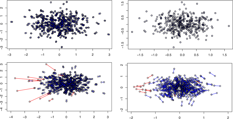
Figure 1: For a single Monte Carlo iterate, we plot the embeddings of the three dissimilarities in the matched (top row, left panel is fJOFC, right panel is 3-MDS) and the anomaly (bottom row, left panel is fJOFC, right panel is 3-MDS) settings. In the matched setting, matched triplets are connected by blue lines. In the anomaly setting, blue lines connect the matched points across the embeddings and red lines connect the ten anomaly points they are “matched” to in the data.

4 Results

In this section we both compare and contrast fJOFC and 3-RSMDS and demonstrate the dramatic run time increase achievable by fJOFC versus JOFC over a variety of real and simulated data examples; note that all run times are measured in seconds. In all examples, the algorithms were implemented on a MacBook Pro with a 2.6 GHz Intel Core i5 processor and 4GB 1600 MHz DDR3 memory.

4.1 3-RSMDS and fJOFC

As mentioned previously, fJOFC can be viewed as a softly constrained version of 3-RSMDS. Herein, through a simple illustrative experiment, we highlight the advantages (and disadvantages) of the fJOFC framework.

Method Runtime1 Stress1 ARI Runtime2 Stress2 ARI2 Conf. Ratio
3-RSMDS 214.52 0.042 0.69 312.39 0.18 0.40 10.29
fJOFC 1.39 0.03 0.66 11.56 0.16 0.57 76.07
Table 2: The average running time (over 25 MC iterates) is shown as Runtime1 (in the matched setting) and Runtime2 (in the anomaly setting). The average final normalized stress is Stress1 (in the matched setting) and Stress2 (in the anomaly setting). In the matched setting, the ARI gives the a measure of the fidelity of the K𝐾K-means clustering of the data into 400 clusters (each should contain the three jitters of the same point). In the anomaly setting, the ARI2 column gives a measure of the fidelity of the K𝐾K-means clustering of the non-anomalous data into 390 clusters (each should contain the three jitters of the same point). Lastly, the Conf. Ratio column gives the ratio of the average distance between the triplets of points that have the anomalies (the ten outlier triplets) and the triplets that are correctly matched in the anomaly setting (the 390 non-outlier triplets).

Let Y400×2𝑌superscript4002Y\in\mathbb{R}^{400\times 2} have rows which are independent 2-dimensional Gaussian((5,5),I2)55subscript𝐼2\big{(}(5,5),I_{2}\big{)} random variables. Letting z=max(Y)min(Y)𝑧𝑌𝑌z=\max(Y)-\min(Y), for i=1,2,3,𝑖123i=1,2,3, we set Yisubscript𝑌𝑖Y_{i} to be Y+Ei𝑌subscript𝐸𝑖Y+E_{i}, with the entries of Eisubscript𝐸𝑖E_{i} being independent Uniform(z/50,z/50)𝑧50𝑧50(-z/50,z/50) random variables, which are also independent across i𝑖i. We set ΔisubscriptΔ𝑖\Delta_{i} to be the interpoint distance matrix of Yisubscript𝑌𝑖Y_{i}. These {Yi}subscript𝑌𝑖\{Y_{i}\} represent our n=400𝑛400n=400 objects measured under m=3𝑚3m=3 modalities. Let Z400×2𝑍superscript4002Z\in\mathbb{R}^{400\times 2} have rows 11,12,,400111240011,12,\ldots,400 identical to those in Y𝑌Y and let the first ten rows of Z𝑍Z be independent 2-dimensional Gaussian((8,8),2I2)882subscript𝐼2\big{(}(8,8),2\cdot I_{2}\big{)} random variables. Let Y4=Z+E4subscript𝑌4𝑍subscript𝐸4Y_{4}=Z+E_{4}, with E4subscript𝐸4E_{4} defined analogously to the Eissuperscriptsubscript𝐸𝑖𝑠E_{i}^{\prime}s above. Let Δ4subscriptΔ4\Delta_{4} be the interpoint distance matrix of Y4subscript𝑌4Y_{4}.

We use fJOFC and the INDSCAL algorithm (for 3-RSMDS, as implemented in the smacof package (Leeuw and Mair, 2008) in R) to embed (Δ1,Δ2,Δ3)subscriptΔ1subscriptΔ2subscriptΔ3(\Delta_{1},\Delta_{2},\Delta_{3}) (the matched setting) and (Δ1,Δ2,Δ4)subscriptΔ1subscriptΔ2subscriptΔ4(\Delta_{1},\Delta_{2},\Delta_{4}) (the anomaly setting). Results are summarized below in Figure 1 and Table 2. In Figure 1, for a single Monte Carlo iterate, we plot the embeddings of the three dissimilarities in the matched (top row, left panel is fJOFC, right panel is 3-MDS) and the anomaly (bottom row, left panel is fJOFC, right panel is 3-MDS) settings. In the matched setting, matched triplets are connected by blue lines. In the anomaly setting, blue lines connect the matched points across the embeddings and red lines connect the ten anomaly points they are “matched” to in the data.

Results over 25 MC iterates are summarized in Table 2. The average running time is shown as Runtime1 (in the matched setting) and Runtime2 (in the anomaly setting). The average final normalized stress is Stress1 (in the matched setting) and Stress2 (in the anomaly setting). In the matched setting, the ARI (adjusted Rand index; see Hubert and Arabie (1985)) a measure of the fidelity of the K𝐾K-means clustering of the data into 400 clusters (each should contain the three jitters of the same point). In the anomaly setting, the column ARI2 gives the a measure of the fidelity of the K𝐾K-means clustering of the non-anomalous data into 390 clusters (each should contain the three jitters of the same non-anomalous point). An ARI of 1 means that the clustering of the embedded points perfectly clusters the repeated observations of the data, while an ARI of 0 indicates that the clustering of the embedded points behaves as chance in recovering the clusters of the repeated observations. Lastly, the Conf. Ratio column gives the ratio of the average distance between the triplets of points that have the anomalies (the ten anomaly triplets) and the triplets that are correctly matched in the anomaly setting (the 390 non-anomaly triplets).
Refer to caption
(a) Matched Setting.
Refer to caption
(b) Anomaly Setting.
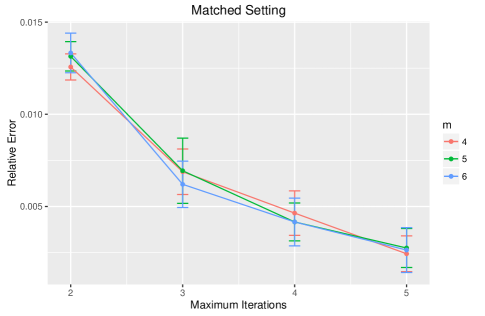
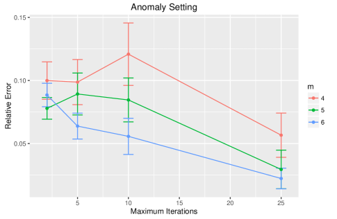
Figure 2: We plot the average (over 25 Monte Carlo iterates) relative error 𝐗(final)𝐗(k)2𝐗(final)2subscriptnormsubscript𝐗finalsubscript𝐗𝑘2subscriptnormsubscript𝐗final2\frac{\|{\bf X}_{(\text{final})}-{\bf X}_{(k)}\|_{2}}{\|{\bf X}_{(\text{final})}\|_{2}} ±2plus-or-minus2\pm 2 s.e. over a range of values of k𝑘k (the x𝑥x-axis in Figure 2(a)). In the left panel, we plot the ratio in the matched setting with m=4,5,6𝑚456m=4,5,6 dissimilarities and in the right panel, we plot the ratio in the anomaly setting with m=4,5,6𝑚456m=4,5,6 dissimilarities, one of which contains the anomaly. Note that in the anomaly setting, only the relative error amongst the n(m1)+(n10)𝑛𝑚1𝑛10n*(m-1)+(n-10) non-anomalous points is plotted.

From this simple experiment, we see that fJOFC is empirically i. much faster than (this off the shelf implementation of) 3-RSMDS; ii. performs comparably to 3-RSMDS when the data are all matched across the modalities with no anomalous behavior—see the ARI column in Table 2; iii. is better able to preserve the correct matchedness in the presence of anomalous data—see the ARI2 and Conf. Ratio columns of Table 2; results which are echoed in Sun and Priebe (2013); Shen et al. (2016)

4.2 Error tolerance

With the same setting as in Section 4.1, we explore the effect of early stopping on the global fJOFC output. As mentioned previously, the sequential Guttman transforms often exhibit good global properties, and good solutions can often be obtained after only a few iterates. To demonstrate this, we plot the relative error (over 25 Monte Carlo iterates) 𝐗(final)𝐗(k)2𝐗(final)2subscriptnormsubscript𝐗finalsubscript𝐗𝑘2subscriptnormsubscript𝐗final2\frac{\|{\bf X}_{(\text{final})}-{\bf X}_{(k)}\|_{2}}{\|{\bf X}_{(\text{final})}\|_{2}} ±2plus-or-minus2\pm 2 s.e. over a range of values of k𝑘k (the x𝑥x-axis in Figure 2(a)). In the left panel, we plot the ratio in the matched setting with m=4,5,6𝑚456m=4,5,6 dissimilarities and in the right panel, we plot the ratio in the anomaly setting with m=4,5,6𝑚456m=4,5,6 dissimilarities, one of which contains the anomaly. Note that in the anomaly setting, only the relative error amongst the n(m1)+(n10)𝑛𝑚1𝑛10n*(m-1)+(n-10) non-anomalous points is plotted. We see that, in the matched setting, very few sequential iterates are needed before the embedding stabilizes. In the anomaly setting—when on average over 100 sequential iterates are needed for the algorithm to terminate with ϵ=106italic-ϵsuperscript106\epsilon=10^{-6} tolerance—we see 5%absentpercent5\approx 5\% relative error with only 25 iterates. Indeed, here and in the real data examples, we find that ϵ=106italic-ϵsuperscript106\epsilon=10^{-6} is often a conservative tolerance level and a sufficiently good embedding can be obtained with far fewer iterates; we are presently investigating methods for adaptively choosing the number of iterates, though we do not pursue this further here.

4.3 JOFC versus fJOFC
Refer to caption
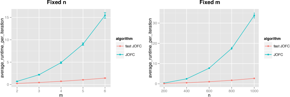
Figure 3: We embed 𝚫nm×nm𝚫superscript𝑛𝑚𝑛𝑚{\bf\Delta}\in\mathbb{R}^{nm\times nm} via fJOFC and JOFC using identical initial configurations 𝐗(0)=subscript𝐗0absent{\bf X}_{(0)}=cMDS(𝚫)𝚫({\bf\Delta}) as in Remark 2. We then plot the average run time (in seconds) per iteration (±2s.e.formulae-sequenceplus-or-minus2𝑠𝑒\pm 2s.e.) versus m𝑚m (left panel) and n𝑛n (right panel) for both JOFC and fJOFC, averaged over 50 Monte Carlo replicates. In the left panel we fix n=400,𝑛400n=400, and vary m=2,3,4,5,6𝑚23456m=2,3,4,5,6. In the right panel, we fix m=3𝑚3m=3 and vary n=200,400,600,800,1000𝑛2004006008001000n=200,400,600,800,1000.

Let Y400×2𝑌superscript4002Y\in\mathbb{R}^{400\times 2} have rows which are independent 2-dimensional Gaussian((5,5),I2)55subscript𝐼2\big{(}(5,5),I_{2}\big{)} random variables. Letting z=max(Y)min(Y)𝑧𝑌𝑌z=\max(Y)-\min(Y), for i=1,2,,6,𝑖126i=1,2,\ldots,6, we set Yisubscript𝑌𝑖Y_{i} to be Y+Ei𝑌subscript𝐸𝑖Y+E_{i}, with the entries of Eisubscript𝐸𝑖E_{i} being independent Uniform(z/50,z/50)𝑧50𝑧50(-z/50,z/50) random variables, which are also independent across i𝑖i. We set ΔisubscriptΔ𝑖\Delta_{i} to be the interpoint distance matrix of Yisubscript𝑌𝑖Y_{i}. These {Yi}subscript𝑌𝑖\{Y_{i}\} represent our n=400𝑛400n=400 objects measured under m=6𝑚6m=6 modalities. For m=2,3,,6,𝑚236m=2,3,\ldots,6, we embed the omnibus matrix 𝚫𝚫\bf\Delta (defined as in Section 1.2.1) into 2superscript2\mathbb{R}^{2} with both fJOFC (in serial) and JOFC using an identical initial configurations 𝐗(0)=cMDS(𝚫),subscript𝐗0cMDS𝚫{\bf X}_{(0)}=\text{cMDS}({\bf\Delta}), as outlined in Remark 2. We plot the average run time per iteration versus m𝑚m for both fJOFC and JOFC in Figure 3 (left panel), averaged over 50 Monte Carlo replicates. Even in this relatively small simulation, the decreased runtime speed is dramatically illustrated, even with fJOFC run in serial. The ratio of the average run times (JOFC versus fJOFC) is (2.86,4.82,6.70,8.59,10.71)2.864.826.708.5910.71(2.86,4.82,6.70,8.59,10.71) for m=(2,3,4,5,6)𝑚23456m=(2,3,4,5,6), which suggests that fJOFC is a factor of m𝑚m (1.6mabsent1.6𝑚\approx 1.6m) faster than JOFC here. This corroborates the runtime results in Section 2; indeed, as here n𝑛n is constant, JOFC has complexity O(m3)𝑂superscript𝑚3O(m^{3}) while fJOFC has complexity O(m2)𝑂superscript𝑚2O(m^{2}).

We next consider the case of fixed m=3𝑚3m=3 and varying n=(200,400,600,800,1000)𝑛2004006008001000n=(200,400,600,800,1000). With Y𝑌Y and 𝚫𝚫\bf\Delta defined as above, we again embed 𝚫nm×nm𝚫superscript𝑛𝑚𝑛𝑚{\bf\Delta}\in\mathbb{R}^{nm\times nm} into 2superscript2\mathbb{R}^{2} via fJOFC (in serial) and JOFC using identical initial configurations 𝐗(0)=subscript𝐗0absent{\bf X}_{(0)}=cMDS(𝚫)𝚫({\bf\Delta}). In Figure 3 (right panel), we plot the average run time per iteration versus n𝑛n for both JOFC and fJOFC, averaged over 50 Monte Carlo replicates. Again, note the dramatic speedup achieved by fJOFC, with the ratio of the average run times (JOFC versus fJOFC) being (2.10,4.86,7.45,10.13,12.63)2.104.867.4510.1312.63(2.10,4.86,7.45,10.13,12.63) for n=(200,400,600,800,1000)𝑛2004006008001000n=(200,400,600,800,1000). This suggests that fJOFC is a factor of n𝑛n (0.12nabsent0.12𝑛\approx 0.12n) faster than JOFC here, which corroborates the runtime results in Section 2; indeed, as here m𝑚m is constant, JOFC has complexity O(n3)𝑂superscript𝑛3O(n^{3}) while fJOFC has complexity O(n2)𝑂superscript𝑛2O(n^{2}).

4.4 Out-of-sample efficiency

Refer to caption
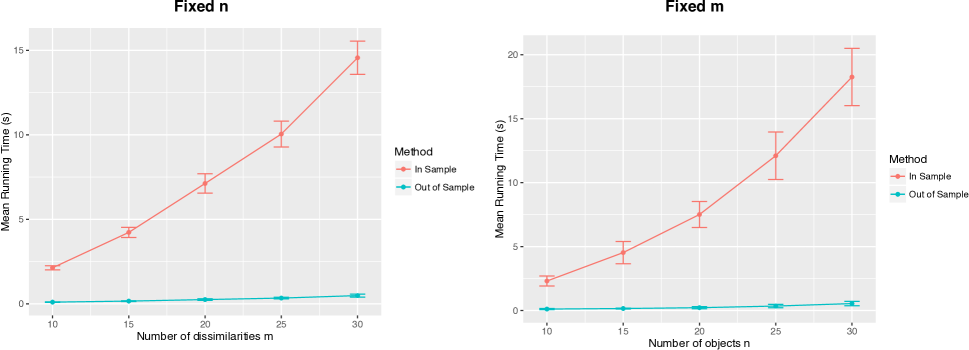
Figure 4: We embed all but one object of 𝚫nm×nm𝚫superscript𝑛𝑚𝑛𝑚{\bf\Delta}\in\mathbb{R}^{nm\times nm} via fJOFC, and use the out-of-sample procedure to embed the final object (m𝑚m views of the n𝑛n-th object). We then plot the average running time (in seconds) ±2s.e.formulae-sequenceplus-or-minus2𝑠𝑒\pm 2s.e. of the in-sample and the out-of-sample procedure versus m𝑚m (left panel) and versus n𝑛n (right panel), averaged over 25 Monte Carlo replicates. In the left panel we fix n=200,𝑛200n=200, and vary m=10,15,20,25,30𝑚1015202530m=10,15,20,25,30. In the right panel, we fix m=10𝑚10m=10 and vary n=200,300,400,500,600𝑛200300400500600n=200,300,400,500,600.

We next demonstrate the efficiency of the out-of-sample fJOFC procedure. With the same data set-up as above (with 333-dimensional Gaussian random variables here, but otherwise identical to the data setup used above), we embed all but one object of 𝚫nm×nm𝚫superscript𝑛𝑚𝑛𝑚{\bf\Delta}\in\mathbb{R}^{nm\times nm} via fJOFC, and use the out-of-sample procedure to embed the final object (m𝑚m views of the n𝑛n-th object). Running time results (in seconds) are plotted in Figure 4, where we plot the average running time (in seconds) ±2s.e.formulae-sequenceplus-or-minus2𝑠𝑒\pm 2s.e. of the in-sample and the out-of-sample procedure versus m𝑚m (left panel) and versus n𝑛n (right panel), averaged over 25 Monte Carlo replicates. In the left panel we fix n=200,𝑛200n=200, and vary m=10,15,20,25,30𝑚1015202530m=10,15,20,25,30. In the right panel, we fix m=10𝑚10m=10 and vary n=200,300,400,500,600𝑛200300400500600n=200,300,400,500,600. As seen previously, the runtime of fJOFC empirically varies quadratically (in n𝑛n for fixed m𝑚m and in m𝑚m for fixed n𝑛n). However, we observe that the runtime of the out-of-sample procedure empirically varies linearly (in n𝑛n for fixed m𝑚m and in m𝑚m for fixed n𝑛n), which agrees with the computational complexity results of Section 3.

In Table 3 we show the sum of the residual errors of the out-of-sample embedding versus the in-sample embedding—i=1m𝐗(final)(i)[n,:]𝐲i2superscriptsubscript𝑖1𝑚subscriptnormsubscriptsuperscript𝐗𝑖final𝑛:subscript𝐲𝑖2\sum_{i=1}^{m}\|{\bf X}^{(i)}_{(\text{final})}[n,:]-{\bf y}_{i}\|_{2}—for fixed n𝑛n and varying m𝑚m (top row) and for fixed m𝑚m and varying n𝑛n (bottom row) averaged over 25 Monte Carlo iterates. For each combination of m𝑚m and n𝑛n, we first embed the full mn×mn𝑚𝑛𝑚𝑛mn\times mn dissimilarity 𝚫𝚫{\bf\Delta} using fJOFC. We next embed all but one of the objects (n1𝑛1n-1 objects over m𝑚m modalities) using fJOFC and the n𝑛n-th object via the out-of-sample procedure of Section 3, and compute the sum of the residual errors between the out-of-sample and the in-sample embeddings of the n𝑛n-th object. We see that, for fixed n𝑛n and varying m𝑚m, the total error is increasing in m𝑚m but negligible on average per modality. As m𝑚m is fixed and n𝑛n varies, the total error is relatively constant, which is unsurprising as, in each case, exactly m𝑚m additional data points are being out-of-sample embedded into a fixed dimensional space.

Sum of Residual Errors of Out-of-Sample Versus In-Sample
m=10𝑚10m=10 m=15𝑚15m=15 m=20𝑚20m=20 m=25𝑚25m=25 m=30𝑚30m=30
n=200𝑛200n=200 0.067 0.121 0.184 0.366 0.364
n=200𝑛200n=200 n=300𝑛300n=300 n=400𝑛400n=400 n=500𝑛500n=500 n=600𝑛600n=600
m=10𝑚10m=10 0.057 0.059 0.101 0.078 0.091
Table 3: The sum of the residual errors of the out-of-sample embedding versus the in-sample embedding—i=1m𝐗(final)(i)[n,:]𝐲i2superscriptsubscript𝑖1𝑚subscriptnormsubscriptsuperscript𝐗𝑖final𝑛:subscript𝐲𝑖2\sum_{i=1}^{m}\|{\bf X}^{(i)}_{(\text{final})}[n,:]-{\bf y}_{i}\|_{2}—for fixed n𝑛n and varying m𝑚m (top row) and for fixed m𝑚m and varying n𝑛n (bottom row) averaged over 25 Monte Carlo iterates.

4.5 Real Data Examples

We next demonstrate the key feature of the JOFC procedure in a pair of real data sets; namely, the ability of the algorithm to preserve cross-modality matchedness while not forcing incommensurate versions of the data points to be artificially embedded close to one another. Indeed, in the JOFC procedure,

  • 1.

    if an object’s properties are well-preserved across the m𝑚m modalities, then the object’s associated m𝑚m points in the configuration will be embedded close to each other;

  • 2.

    if an object’s properties are not well-preserved across the m𝑚m modalities, then JOFC (with well-chosen w𝑤w) will not artificially force the object’s m𝑚m incommensurate configuration points to be close to each other in the embedding.

Incommensurate embeddings can inform both how and why the data modalities differ. By studying these pathologies further, we aim to better understand the data features that are emphasized in one modality versus another, which is crucial for understanding potential benefits from pursuing further inference in the joint (versus single) embedding space.

We explore this further below in a data set derived from the French and English Wikipedia graphs and in a time series of zebrafish calcium ion brain images from Prevedel et al. (2014).
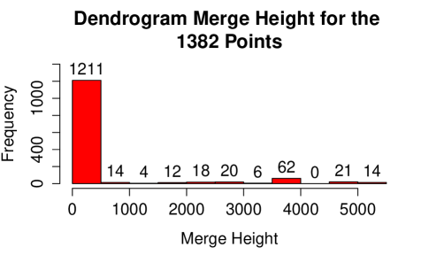
Refer to caption
(a) Dendrogram merge heights, all n=1382𝑛1382n=1382 points.
Refer to caption
(b) Dendrogram merge heights for the n=1055𝑛1055n=1055 points with merge height <100absent100<100.
Figure 5: Histograms showing, for each of the n=1382𝑛1382n=1382 points in (a) and for each of the 105510551055 points with merge height <100absent100<100 in (b), the height in the hierarchical clustering dendrogram when each of the four modalities was first merged into a single cluster for that point.

4.5.1 Wikipedia

We collect the n=𝑛absentn=1382 articles {y1i}i=11382superscriptsubscriptsubscript𝑦1𝑖𝑖11382\{y_{1i}\}_{i=1}^{1382} from English Wikipedia which compose the 2-hop neighborhood of the article entitled “Algebraic Geometry” (where articles are linked if there exists a hyperlink in one article to the other, and these links are considered undirected). There is a natural 111-111 correspondence between these articles and their versions in French Wikipedia, and we will denote the associated French articles by {y2i}i=11382superscriptsubscriptsubscript𝑦2𝑖𝑖11382\{y_{2i}\}_{i=1}^{1382}.

As in Shen et al. (2016), each {yji}i=11382superscriptsubscriptsubscript𝑦𝑗𝑖𝑖11382\{y_{ji}\}_{i=1}^{1382} for j=1,2𝑗12j=1,2, further gives rise to two measures of inter-article dissimilarity: Δj1subscriptΔ𝑗1\Delta_{j1}, the shortest path distance in the undirected hyperlink graph; and Δj2subscriptΔ𝑗2\Delta_{j2}, the cosine dissimilarities between text feature vectors (provided by latent semantic indexing, see Deerwester et al. (1990) for detail) associated with each article. We use fJOFC—with w=10𝑤10w=10 as suggested by Adali and Priebe (2015)—to embed these n=1382𝑛1382n=1382 points across m=4𝑚4m=4 modalities into 10.superscript10\mathbb{R}^{10}. Note that implementing our fJOFC algorithm in serial ran in \approx42.2 minutes while the JOFC algorithm with the same settings ran in \approx10.37 hours (a factor of \approx14.7 speedup).

In this omnibus embedding, if all 4 embedded versions of a single Wikipedia article lie close together, then this article’s relationship to all of the other articles is preserved across modality. If any of the 4 embedded versions is incommensurate with the others then this would indicate either:

  • i.

    The text features of the article differ significantly across language; i.e. the associated row of 𝐗i(2)superscriptsubscript𝐗𝑖2{\bf X}_{i}^{(2)}, the embedding associated with Δ12subscriptΔ12\Delta_{12}, is far from 𝐗i(4)superscriptsubscript𝐗𝑖4{\bf X}_{i}^{(4)}, the embedding associated with Δ22subscriptΔ22\Delta_{22}. While the French articles are not translations of their English counterparts (or vice versa), further understanding the textual feature highlighted by these incommensurabilities would be useful before pursuing further inference (e.g. topic modeling) in the joint embedding.

  • ii.

    The hyperlink graph structure is not preserved across modality; i.e. the associated row of 𝐗i(1)superscriptsubscript𝐗𝑖1{\bf X}_{i}^{(1)}, the embedding associated with Δ11subscriptΔ11\Delta_{11}, is far from 𝐗i(3)superscriptsubscript𝐗𝑖3{\bf X}_{i}^{(3)}, the embedding associated with Δ21subscriptΔ21\Delta_{21}.

  • iii.

    The hyperlink structure and the textual similarities are incommensurate; i.e. the associated row of 𝐗i(1)superscriptsubscript𝐗𝑖1{\bf X}_{i}^{(1)}, the embedding associated with Δ11subscriptΔ11\Delta_{11}, is far from 𝐗i(2)superscriptsubscript𝐗𝑖2{\bf X}_{i}^{(2)}, the embedding associated with Δ12subscriptΔ12\Delta_{12}, or the associated row of 𝐗i(3)superscriptsubscript𝐗𝑖3{\bf X}_{i}^{(3)}, the embedding associated with Δ21subscriptΔ21\Delta_{21}, is far from 𝐗i(4)superscriptsubscript𝐗𝑖4{\bf X}_{i}^{(4)}, the embedding associated with Δ22subscriptΔ22\Delta_{22}. By studying these incommensurabilities further, we hope to better understand the data features that are emphasized by graph-based versus text-feature-based methodologies.

To investigate further, we proceed by hierarchically clustering (using Ward’s method, see Johnson (1967) for detail) the 4×1382413824\times 1382 points of the omnibus embedding and then compute the pairwise cophenetic distance (the height in the resulting dendrogram at which the two points are first clustered together) between each of the points. If the dissimilarities are well preserved across modality, then the maximum cophenetic distance between two embedded versions of the same article (we call this the Dendrogram Merge Height or DMH) should be small.
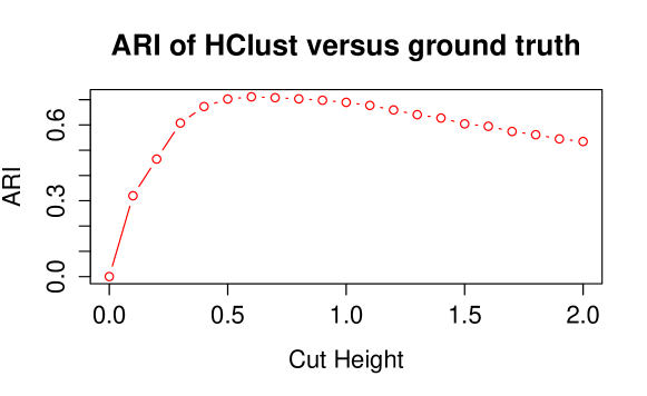
Refer to caption
Figure 6: The adjusted Rand index between the clusters given by the hierarchical clustering dendrogram at height h[0,2]02h\in[0,2] and the ground truth clustering (given by the 1382 size 4 clusters each composed of a single article across modalities).

In Figure 5(a), we plot a histogram of the DMH’s for the 1382 articles, and note that over 76%percent\% of the articles have DMH less than 100. In Figure 5(b) we see that over 63%percent\% of the articles have DMH less than 10. To further confirm that the dissimilarities are well preserved across modality, we calculated cluster labels given by the hierarchical clustering dendrogram at height h[0,2]02h\in[0,2]. We then compute the adjusted Rand index, ARI (see Hubert and Arabie, 1985), between these clusterings and the ground truth clustering (given by the 1382 size 4 clusters each composed of a single article across modalities), and plot this in Figure 6. From the figure, we see that the clustering is not only grossly clustering the article 4-tuples together, but is also capturing the fine-grain differences between the different articles as well.

If the ARI between the hierarchical clustering and the ground truth clustering was equal to 1, then the structure of the four dissimilarities would be nearly identical, and joint inference across modality would yield minimal gain over separately embedding the ΔisubscriptΔ𝑖\Delta_{i}’s and then applying subsequent inference methodologies.
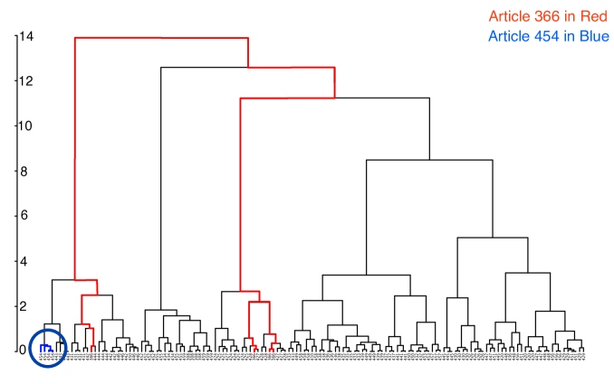
Refer to caption
Figure 7: A branch of the hierarchical clustering dendrogram when the tree is cut at height 20. Note that the four modality-specific embeddings of article 454 (highlighted in blue in the dendrogram) are very similar, while those of article 366 are not (the English graph with shortest path distance differs significantly from the other three modalities for this point).

From Figures 5(a)-5(b) and 6, we see this is not the case. Indeed, we see that the text-feature-based methods and graph-based methods are emphasizing some different data features both within and across language, and therefore for some articles the relative geometry in the four modality-specific embeddings is not commensurate. We illustrate this in Figure 7, where we plot a branch of the hierarchical clustering dendrogram when the tree is cut at height 20. Note that although the four modality-specific embeddings of many articles (article 454 is highlighted here in blue as an example) are very similar, some of the articles’ embeddings are not preserved well across modality (article 366 is highlighted here in red as an example; note that the English graph with shortest path distance differs significantly from the other three modalities for this article).

4.5.2 Zebrafish brains

In Prevedel et al. (2014), the authors combined Light-Field Deconvolution Microscopy and pan-neuronal expression of GCaMP, a fluorescent calcium indicator that serves as a proxy for neuronal activity, to produce a time series of whole-brain zebrafish neuronal activity at near single neuron resolution. The data consists of 5000 realizations of a multivariate time series {Z(t)}t=15000superscriptsubscriptsuperscript𝑍𝑡𝑡15000\{Z^{(t)}\}_{t=1}^{5000} with Z(t)5379superscript𝑍𝑡superscript5379Z^{(t)}\in\mathbb{R}^{5379} for all t𝑡t, where for each i[5379],Z(t)(i)formulae-sequence𝑖delimited-[]5379superscript𝑍𝑡𝑖i\in[5379],\,Z^{(t)}(i)\in\mathbb{R} represents the activity of neuron i𝑖i at time t𝑡t. Each time frame [t,t+1)𝑡𝑡1[t,t+1) is 1/201201/20 of a second; i.e. the data was collected at 20 Hz. After preprocessing the data and removing some artificial edge neurons, we are left with Z(t)5105superscript𝑍𝑡superscript5105Z^{(t)}\in\mathbb{R}^{5105} for each of t=1,2,,5000𝑡125000t=1,2,\ldots,5000.

Refer to caption
Figure 8: Heatmaps of the Frobenius norm differences between the 202020 zebrafish neuron embeddings {𝐗(τ)}τ=1130superscriptsubscriptsuperscript𝐗𝜏𝜏1130\{{\bf X}^{(\tau)}\}_{\tau=11}^{30} obtained by fJOFC over a range of w𝑤w’s. Each heatmap is a 20×20202020\times 20 grid, where the intensity of the i,j𝑖𝑗i,j-th entry indicates the difference between the embeddings of the nsuperscript𝑛n^{*} fish neurons at times τ=i𝜏𝑖\tau=i and τ=j𝜏𝑗\tau=j; more red indicates less difference in the embedded space and white indicating very different embeddings. Note the anomalous point at τ=23.𝜏23\tau=23.

Binning the time stamps into 100100100 overlapping periods of 555 seconds (so that for each τ[100],𝜏delimited-[]100\tau\in[100], bin τ𝜏\tau consists of the matrix of observations

𝐙(τ)=[Z(50(τ1)+1)||Z(50(τ+1)]=[(𝐙1(τ))|(𝐙2(τ))||(𝐙5105(τ))]5105×100),{\bf Z}^{(\tau)}=[Z^{(50(\tau-1)+1)}|\cdots|Z^{(50(\tau+1)}]=\left[({\bf Z}^{(\tau)}_{1})^{\top}|({\bf Z}^{(\tau)}_{2})^{\top}|\cdots|({\bf Z}^{(\tau)}_{5105})^{\top}\right]^{\top}\in\mathbb{R}^{5105\times 100}),

we compute a time series of 100 dissimilarity matrices {Δ(τ)}τ=1100superscriptsubscriptsuperscriptΔ𝜏𝜏1100\{\Delta^{(\tau)}\}_{\tau=1}^{100} as follows. For each τ𝜏\tau, we compute the thresholded correlation matrix D(τ)5105×5105superscript𝐷𝜏superscript51055105D^{(\tau)}\in\mathbb{R}^{5105\times 5105} with

Di,j(τ)=𝟙{|corr(𝐙i(τ),𝐙j(τ))|>0.7}subscriptsuperscript𝐷𝜏𝑖𝑗1corrsubscriptsuperscript𝐙𝜏𝑖subscriptsuperscript𝐙𝜏𝑗0.7D^{(\tau)}_{i,j}=\mathbbm{1}\{|\text{corr}({\bf Z}^{(\tau)}_{i},{\bf Z}^{(\tau)}_{j})|>0.7\}

(where the threshold 0.70.70.7 was chosen to ensure sufficient sparsity in the resulting D(τ)superscript𝐷𝜏D^{(\tau)}’s). These correlation matrices are then transformed to dissimilarity matrices {Δ(τ)}τ=1100superscriptsubscriptsuperscriptΔ𝜏𝜏1100\{\Delta^{(\tau)}\}_{\tau=1}^{100} by defining

Δi,j(τ)=1|Nτ(i)Nτ(i)||Nτ(i)Nτ(i)|,subscriptsuperscriptΔ𝜏𝑖𝑗1subscript𝑁𝜏𝑖subscript𝑁𝜏𝑖subscript𝑁𝜏𝑖subscript𝑁𝜏𝑖\Delta^{(\tau)}_{i,j}=1-\frac{|N_{\tau}(i)\cap N_{\tau}(i)|}{|N_{\tau}(i)\cup N_{\tau}(i)|},

where Nτ(i)subscript𝑁𝜏𝑖N_{\tau}(i) is the neighborhood of neuron i𝑖i in D(τ)superscript𝐷𝜏D^{(\tau)} viewed as a graph.

Initial change point detection analysis, analogous to that in Park et al. (2015), indicated that there was an anomaly in the neural correlations at time τ=23superscript𝜏23\tau^{*}=23 and identified n=469superscript𝑛469n^{*}=469 neurons responsible for this anomaly. To explore this further, we use fJOFC to embed a portion of the time series (from times τ=11𝜏11\tau=11 to τ=30𝜏30\tau=30) obtaining the configuration

𝐗=[(𝐗(11))|(𝐗(12))||(𝐗(30))].superscript𝐗topsuperscriptdelimited-[]conditionalsuperscriptsuperscript𝐗11topsuperscriptsuperscript𝐗12topsuperscriptsuperscript𝐗30toptop{\bf X}^{\top}=[({\bf X}^{(11)})^{\top}|({\bf X}^{(12)})^{\top}|\cdots|({\bf X}^{(30)})^{\top}]^{\top}.

If there is an anomaly in the activity of the nsuperscript𝑛n^{*} neurons at τ=23superscript𝜏23\tau^{*}=23, this should be evinced by 𝐗(23)superscript𝐗23{\bf X}^{(23)} significantly differing from 𝐗(τ)superscript𝐗𝜏{\bf X}^{(\tau)} for τ23𝜏23\tau\neq 23, as seen in Figures 8 and 9. Moreover, the embedding can also inform the structure of the anomaly, as we can identify the change in structure within the n=469superscript𝑛469n^{*}=469 neurons which is responsible for the anomaly in the embedded space; see Figure 10. Below, we expound on the details of our embedding procedure and findings.
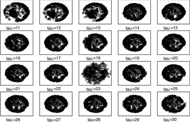
Refer to caption
Figure 9: Embeddings of the m=20𝑚20m=20 elements of the time-series {Δ~(τ)}τ=1130superscriptsubscriptsuperscript~Δ𝜏𝜏1130\{\widetilde{\Delta}^{(\tau)}\}_{\tau=11}^{30} into 2superscript2\mathbb{R}^{2} obtained via fJOFC with w=10𝑤10w=10. Each of the 202020 plots is on the same set of axes. Note the anomaly at τ=23𝜏23\tau=23.

Restricting the full dissimilarities to the nsuperscript𝑛n^{*} identified anomalous neurons—yielding a times series {Δ~(τ)}τ=1100superscriptsubscriptsuperscript~Δ𝜏𝜏1100\{\widetilde{\Delta}^{(\tau)}\}_{\tau=1}^{100} of 100100100 dissimilarities in 469×469superscript469469\mathbb{R}^{469\times 469}—we first embed the m=20𝑚20m=20 elements of {Δ~(τ)}τ=1130superscriptsubscriptsuperscript~Δ𝜏𝜏1130\{\widetilde{\Delta}^{(\tau)}\}_{\tau=11}^{30} into 2superscript2\mathbb{R}^{2}. To test if there is an anomaly at τ=23𝜏23\tau=23, we next compute the Frobenius norm differences between the 202020 embeddings {𝐗(τ)}τ=1130superscriptsubscriptsuperscript𝐗𝜏𝜏1130\{{\bf X}^{(\tau)}\}_{\tau=11}^{30} in the configuration. Results are summarized in Figure 8, where we plot a heatmap of the Frobenius norm differences between the {𝐗(τ)}τ=1130superscriptsubscriptsuperscript𝐗𝜏𝜏1130\{{\bf X}^{(\tau)}\}_{\tau=11}^{30} over a range of w𝑤w’s (plots of the 2-dimensional fJOFC embeddings with w=10𝑤10w=10 across τ=11,12,,30𝜏111230\tau=11,12,\ldots,30 are displayed in Figure 9). Each heatmap is a 20×20202020\times 20 grid, where the intensity of the i,j𝑖𝑗i,j-th entry indicates the difference between the embeddings of the nsuperscript𝑛n^{*} fish neurons in 𝐗(i)superscript𝐗𝑖{\bf X}^{(i)} and 𝐗(j)superscript𝐗𝑗{\bf X}^{(j)}; more red indicates less difference in the embedded space and white indicating very different embeddings. We see that, across the range of w𝑤w’s, there is a significant anomaly in the embedding at τ=23𝜏23\tau=23. This both confirms the initial findings of an anomaly at τ=23𝜏23\tau=23 and demonstrates the potential robustness of this anomaly-detection procedure to misspecified w𝑤w. We also note that the embeddings at times τ=11,12,13𝜏111213\tau=11,12,13 are significantly different from the embeddings at all other times. Further analysis is needed to determine if this is neuroscientifically significant or a data collect/algorithmic artifact. We lastly note that this embedding ran in 1.5absent1.5\approx 1.5 hours using fJOFC run in serial and over 202020 hours using JOFC, again showing the dramatic speedup of our fJOFC procedure.

To further understand the structure of this anomaly, we plot the change in the embeddings from times 21–22, times 22–23, times 23–24, and times 24–25 in Figure 10 (so that there are 2n2superscript𝑛2n^{*} points in each panel). In the figure, the neurons in the configuration at time 23 are displayed as red points, with neurons in the configuration at other times displayed as black points. For each individual neuron, the movement in the configuration from times τ𝜏\tau to τ+1𝜏1\tau+1 are highlighted with blue lines; i.e., there is a line connecting the position of the neuron at time τ𝜏\tau to its position at time τ+1𝜏1\tau+1. From this figure, we can identify the groups of neurons whose change in activity is responsible for the anomaly. Again, further analysis is necessary to determine the potential neuroscientific significance of these neurons’ activity.
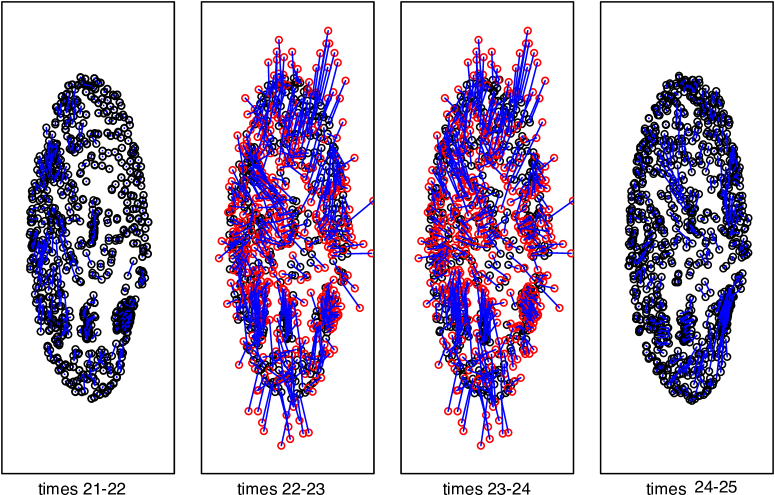
Refer to caption
Figure 10: Plot of the change in the embeddings from times 21–22, times 22–23, times 23–24, and times 24–25 (so that there are 2n2superscript𝑛2n^{*} points in each panel). In the figure, the neurons in the configuration at time 23 are displayed as red points, with neurons in the configuration at other times displayed as black points. For each individual neuron, the movement in the configuration from times τ𝜏\tau to τ+1𝜏1\tau+1 are highlighted with blue lines; i.e., there is a line connecting the position of the neuron at time τ𝜏\tau to its position at time τ+1𝜏1\tau+1.

5 Conclusion

The JOFC algorithm has proven to be a valuable and adaptable tool for a variety of inference tasks (e.g., graph matching (Lyzinski et al., 2013); hypothesis testing (Priebe et al., 2013); joint classification (Sun and Priebe, 2013); among others). The key capability enabled by our fJOFC algorithm (both in-sample and out-of-sample) versus the JOFC algorithm is enhanced scalability in m𝑚m and n𝑛n; indeed, for a fixed n𝑛n, we see a factor of m𝑚m speedup over the JOFC algorithm, and for a fixed m𝑚m we see a factor of n𝑛n speed up achieved by fJOFC. Additionally, the out-of-sample fJOFC procedure is shown to have linear runtime in n𝑛n. Combined with sparse dissimilarity representations of very large data sets, this capability to simultaneously embed many different large dissimilarities, both in and out-of-sample, enables the complex structure of the data to more easily be interrogated, leading to potentially significant discoveries heretofore beyond our grasp.

While the sequential Guttman transforms computed in Algorithm 1 are only guaranteed to converge to a stationary configuration, because the sequence of raw stress values is decreasing, in practice they will typically converge to a local minimizer of σ(𝐗)𝜎𝐗{\bf\sigma(X)}. Note that, in most cases, the local convergence rate of the iterative Guttman transforms is linear, see de Leeuw (1988). In practice, the sequential Guttman transforms often exhibit good global properties, and only a few iterations are required to obtain a sufficiently good suboptimal embedding, see Kearsley et al. (1995). Analyzing these global properties and/or modifying fJOFC to accelerate the linear convergence—for example, by incorporating relaxed updates in the iterative majorization as in De Leeuw and Heiser (1980)—are essential next steps for further scaling fJOFC to very big data.

Appendix A Derivation of 𝐋superscript𝐋\bf L^{\dagger}

In this section, we collect supporting results to derive the desired form of 𝐋superscript𝐋\bf L^{\dagger}. We first prove that 𝐋superscript𝐋{\bf L}^{\dagger} can be realized via 𝐋=(𝐋+1mnJmn)11mnJmnsuperscript𝐋superscript𝐋1𝑚𝑛subscript𝐽𝑚𝑛11𝑚𝑛subscript𝐽𝑚𝑛{\bf L}^{\dagger}=\left({\bf L}+\frac{1}{mn}J_{mn}\right)^{-1}-\frac{1}{mn}J_{mn},

Proposition 9.

Let 𝐖𝐖{\bf W} be any symmetric weight matrix in mn×mnsuperscript𝑚𝑛𝑚𝑛\mathbb{R}^{mn\times mn}. If 𝐋𝐋{\bf L} is the combinatorial Laplacian of 𝐖𝐖{\bf W}, then 𝐋𝐋{\bf L} can be equivalently realized via

𝐋=(𝐋+1mnJmn)11mnJmn.superscript𝐋superscript𝐋1𝑚𝑛subscript𝐽𝑚𝑛11𝑚𝑛subscript𝐽𝑚𝑛{\bf L}^{\dagger}=\left({\bf L}+\frac{1}{mn}J_{mn}\right)^{-1}-\frac{1}{mn}J_{mn}. (17)
Proof.

The proof is straightforward linear algebra, but we include it here for completeness. We first note that Jmn𝐋=𝐋Jmn=0subscript𝐽𝑚𝑛𝐋𝐋subscript𝐽𝑚𝑛0J_{mn}{\bf L}={\bf L}J_{mn}=0, so that

(𝐋+1mnJmn)Jmn=Jmn=Jmn(𝐋+1mnJmn).𝐋1𝑚𝑛subscript𝐽𝑚𝑛subscript𝐽𝑚𝑛subscript𝐽𝑚𝑛subscript𝐽𝑚𝑛𝐋1𝑚𝑛subscript𝐽𝑚𝑛\left({\bf L}+\frac{1}{mn}J_{mn}\right)J_{mn}=J_{mn}=J_{mn}\left({\bf L}+\frac{1}{mn}J_{mn}\right).

We then calculate

𝐋[(𝐋+1mnJmn)11mnJmn]𝐋𝐋delimited-[]superscript𝐋1𝑚𝑛subscript𝐽𝑚𝑛11𝑚𝑛subscript𝐽𝑚𝑛𝐋\displaystyle{\bf L}\left[\left({\bf L}+\frac{1}{mn}J_{mn}\right)^{-1}-\frac{1}{mn}J_{mn}\right]{\bf L} =𝐋(𝐋+1mnJmn)1𝐋absent𝐋superscript𝐋1𝑚𝑛subscript𝐽𝑚𝑛1𝐋\displaystyle={\bf L}\left({\bf L}+\frac{1}{mn}J_{mn}\right)^{-1}{\bf L}
=𝐋(𝐋+1mnJmn)1(𝐋+1mnJmn1mnJmn)absent𝐋superscript𝐋1𝑚𝑛subscript𝐽𝑚𝑛1𝐋1𝑚𝑛subscript𝐽𝑚𝑛1𝑚𝑛subscript𝐽𝑚𝑛\displaystyle={\bf L}\left({\bf L}+\frac{1}{mn}J_{mn}\right)^{-1}\left({\bf L}+\frac{1}{mn}J_{mn}-\frac{1}{mn}J_{mn}\right)
=𝐋(Imn1mnJmn)=𝐋;absent𝐋subscript𝐼𝑚𝑛1𝑚𝑛subscript𝐽𝑚𝑛𝐋\displaystyle={\bf L}\left(I_{mn}-\frac{1}{mn}J_{mn}\right)={\bf L};

and

[(𝐋+1mnJmn)11mnJmn]𝐋[(𝐋+1mnJmn)11mnJmn]delimited-[]superscript𝐋1𝑚𝑛subscript𝐽𝑚𝑛11𝑚𝑛subscript𝐽𝑚𝑛𝐋delimited-[]superscript𝐋1𝑚𝑛subscript𝐽𝑚𝑛11𝑚𝑛subscript𝐽𝑚𝑛\displaystyle\left[\left({\bf L}+\frac{1}{mn}J_{mn}\right)^{-1}-\frac{1}{mn}J_{mn}\right]{\bf L}\left[\left({\bf L}+\frac{1}{mn}J_{mn}\right)^{-1}-\frac{1}{mn}J_{mn}\right]
=[(𝐋+1mnJmn)11mnJmn](𝐋+1mnJmn1mnJmn)[(𝐋+1mnJmn)11mnJmn]absentdelimited-[]superscript𝐋1𝑚𝑛subscript𝐽𝑚𝑛11𝑚𝑛subscript𝐽𝑚𝑛𝐋1𝑚𝑛subscript𝐽𝑚𝑛1𝑚𝑛subscript𝐽𝑚𝑛delimited-[]superscript𝐋1𝑚𝑛subscript𝐽𝑚𝑛11𝑚𝑛subscript𝐽𝑚𝑛\displaystyle=\left[\left({\bf L}+\frac{1}{mn}J_{mn}\right)^{-1}-\frac{1}{mn}J_{mn}\right]\left({\bf L}+\frac{1}{mn}J_{mn}-\frac{1}{mn}J_{mn}\right)\left[\left({\bf L}+\frac{1}{mn}J_{mn}\right)^{-1}-\frac{1}{mn}J_{mn}\right]
=[Imn21mnJmn+1mnJmn][(𝐋+1mnJmn)11mnJmn]=(𝐋+1mnJmn)11mnJmn;absentdelimited-[]subscript𝐼𝑚𝑛21𝑚𝑛subscript𝐽𝑚𝑛1𝑚𝑛subscript𝐽𝑚𝑛delimited-[]superscript𝐋1𝑚𝑛subscript𝐽𝑚𝑛11𝑚𝑛subscript𝐽𝑚𝑛superscript𝐋1𝑚𝑛subscript𝐽𝑚𝑛11𝑚𝑛subscript𝐽𝑚𝑛\displaystyle=\left[I_{mn}-2\frac{1}{mn}J_{mn}+\frac{1}{mn}J_{mn}\right]\left[\left({\bf L}+\frac{1}{mn}J_{mn}\right)^{-1}-\frac{1}{mn}J_{mn}\right]=\left({\bf L}+\frac{1}{mn}J_{mn}\right)^{-1}-\frac{1}{mn}J_{mn};

and [(𝐋+1mnJmn)11mnJmn]𝐋=Imn1mnJmn=𝐋[(𝐋+1mnJmn)11mnJmn]delimited-[]superscript𝐋1𝑚𝑛subscript𝐽𝑚𝑛11𝑚𝑛subscript𝐽𝑚𝑛𝐋subscript𝐼𝑚𝑛1𝑚𝑛subscript𝐽𝑚𝑛𝐋delimited-[]superscript𝐋1𝑚𝑛subscript𝐽𝑚𝑛11𝑚𝑛subscript𝐽𝑚𝑛\left[\left({\bf L}+\frac{1}{mn}J_{mn}\right)^{-1}-\frac{1}{mn}J_{mn}\right]{\bf L}=I_{mn}-\frac{1}{mn}J_{mn}={\bf L}\left[\left({\bf L}+\frac{1}{mn}J_{mn}\right)^{-1}-\frac{1}{mn}J_{mn}\right] is Hermitian. It follows that 𝐋=(𝐋+1mnJmn)11mnJmnsuperscript𝐋superscript𝐋1𝑚𝑛subscript𝐽𝑚𝑛11𝑚𝑛subscript𝐽𝑚𝑛{\bf L}^{\dagger}=\left({\bf L}+\frac{1}{mn}J_{mn}\right)^{-1}-\frac{1}{mn}J_{mn} as desired. ∎

We have that the combinatorial Laplacian of 𝐖𝐖{\bf W} is given by 𝐋=𝒲Indiag(wi,i)Jn𝐋tensor-product𝒲subscript𝐼𝑛tensor-productdiagsubscript𝑤𝑖𝑖subscript𝐽𝑛{\bf L}=\mathcal{W}\otimes I_{n}-\text{diag}(w_{i,i})\otimes J_{n}. It follows that

𝐋+1mnJmn=𝒲In+(1mnJmdiag(wi,i))Jn.𝐋1𝑚𝑛subscript𝐽𝑚𝑛tensor-product𝒲subscript𝐼𝑛tensor-product1𝑚𝑛subscript𝐽𝑚diagsubscript𝑤𝑖𝑖subscript𝐽𝑛{\bf L}+\frac{1}{mn}J_{mn}=\mathcal{W}\otimes I_{n}+\left(\frac{1}{mn}J_{m}-\text{diag}(w_{i,i})\right)\otimes J_{n}.

Proposing that (𝐋+1mnJmn)1superscript𝐋1𝑚𝑛subscript𝐽𝑚𝑛1({\bf L}+\frac{1}{mn}J_{mn})^{-1} is of the form 𝒱In+𝒵Jn,tensor-product𝒱subscript𝐼𝑛tensor-product𝒵subscript𝐽𝑛\mathcal{V}\otimes I_{n}+\mathcal{Z}\otimes J_{n}, we arrive at the following.

Theorem 10.

With notation as above, let 𝐖𝐖{\bf W} be a weight matrix of the form of Eq. (9), and assume that wi,i>0subscript𝑤𝑖𝑖0w_{i,i}>0 for all i{1,2,,m}𝑖12𝑚i\in\{1,2,\ldots,m\}. Let 𝐋𝐋{\bf L} be the combinatorial Laplacian of 𝐖𝐖{\bf W}, then

(𝐋+1mnJmn)1=(𝒲In+(1mnJmdiag(wi,i))Jn)1=𝒱In+𝒵Jn,superscript𝐋1𝑚𝑛subscript𝐽𝑚𝑛1superscripttensor-product𝒲subscript𝐼𝑛tensor-product1𝑚𝑛subscript𝐽𝑚diagsubscript𝑤𝑖𝑖subscript𝐽𝑛1tensor-product𝒱subscript𝐼𝑛tensor-product𝒵subscript𝐽𝑛\left({\bf L}+\frac{1}{mn}J_{mn}\right)^{-1}=\left(\mathcal{W}\otimes I_{n}+\left(\frac{1}{mn}J_{m}-\text{diag}(w_{i,i})\right)\otimes J_{n}\right)^{-1}=\mathcal{V}\otimes I_{n}+\mathcal{Z}\otimes J_{n},

where 𝒱=𝒲1𝒱superscript𝒲1\mathcal{V}=\mathcal{W}^{-1} and 𝒵=(𝒲+n(1mnJmdiag(wi,i)))1(1mnJmdiag(wi,i))𝒲1.𝒵superscript𝒲𝑛1𝑚𝑛subscript𝐽𝑚diagsubscript𝑤𝑖𝑖11𝑚𝑛subscript𝐽𝑚diagsubscript𝑤𝑖𝑖superscript𝒲1{}\mathcal{Z}=-\left(\mathcal{W}+n\left(\frac{1}{mn}J_{m}-\text{diag}(w_{i,i})\right)\right)^{-1}\left(\frac{1}{mn}J_{m}-\text{diag}(w_{i,i})\right)\mathcal{W}^{-1}.

Proof.

First note that the assumption on {wi,i}i=1msuperscriptsubscriptsubscript𝑤𝑖𝑖𝑖1𝑚\{w_{i,i}\}_{i=1}^{m} assures that 𝒲𝒲\mathcal{W} is strictly diagonally dominant and is therefore invertible. If the proposed form, (𝐋+1mnJmn)1=𝒱In+𝒵Jn,superscript𝐋1𝑚𝑛subscript𝐽𝑚𝑛1tensor-product𝒱subscript𝐼𝑛tensor-product𝒵subscript𝐽𝑛({\bf L}+\frac{1}{mn}J_{mn})^{-1}=\mathcal{V}\otimes I_{n}+\mathcal{Z}\otimes J_{n}, is correct then

Imnsubscript𝐼𝑚𝑛\displaystyle I_{mn} =(𝐋+1mnJmn)(𝐋+1mnJmn)1absent𝐋1𝑚𝑛subscript𝐽𝑚𝑛superscript𝐋1𝑚𝑛subscript𝐽𝑚𝑛1\displaystyle=\left({\bf L}+\frac{1}{mn}J_{mn}\right)\left({\bf L}+\frac{1}{mn}J_{mn}\right)^{-1}
=(𝒲In+(1mnJmdiag(wi,i))Jn)(𝒱In+𝒵Jn,)\displaystyle=\left(\mathcal{W}\otimes I_{n}+\left(\frac{1}{mn}J_{m}-\text{diag}(w_{i,i})\right)\otimes J_{n}\right)\left(\mathcal{V}\otimes I_{n}+\mathcal{Z}\otimes J_{n},\right)
=(𝒲𝒱)In+((𝒲+n(1mnJmdiag(wi,i)))𝒵+(1mnJmdiag(wi,i))𝒱)Jnabsenttensor-product𝒲𝒱subscript𝐼𝑛tensor-product𝒲𝑛1𝑚𝑛subscript𝐽𝑚diagsubscript𝑤𝑖𝑖𝒵1𝑚𝑛subscript𝐽𝑚diagsubscript𝑤𝑖𝑖𝒱subscript𝐽𝑛\displaystyle=(\mathcal{W}\mathcal{V})\otimes I_{n}+\left(\left(\mathcal{W}+n\left(\frac{1}{mn}J_{m}-\text{diag}(w_{i,i})\right)\right)\mathcal{Z}+\left(\frac{1}{mn}J_{m}-\text{diag}(w_{i,i})\right)\mathcal{V}\right)\otimes J_{n}

From this, the desired forms of 𝒱𝒱\mathcal{V} and 𝒵𝒵\mathcal{Z} follow immediately. ∎

From Theorem 10, the following Corollary is immediate:

Corollary 11.

With notation as above, let 𝐖𝐖{\bf W} be a weight matrix of the form of Eq. (9), and assume that wi,i>0subscript𝑤𝑖𝑖0w_{i,i}>0 for all i{1,2,,m}𝑖12𝑚i\in\{1,2,\ldots,m\}. Let 𝐋𝐋{\bf L} be the combinatorial Laplacian of 𝐖𝐖{\bf W}, then

𝐋=𝒲1In+[(𝒲+n(Jmmndiag(wi,i)))1(Jmmndiag(wi,i))𝒲1Jmmn]Jn.superscript𝐋tensor-productsuperscript𝒲1subscript𝐼𝑛tensor-productdelimited-[]superscript𝒲𝑛subscript𝐽𝑚𝑚𝑛diagsubscript𝑤𝑖𝑖1subscript𝐽𝑚𝑚𝑛diagsubscript𝑤𝑖𝑖superscript𝒲1subscript𝐽𝑚𝑚𝑛subscript𝐽𝑛{\bf L}^{\dagger}=\mathcal{W}^{-1}\otimes I_{n}+\left[-\left(\mathcal{W}+n\left(\frac{J_{m}}{mn}-\text{diag}(w_{i,i})\right)\right)^{-1}\left(\frac{J_{m}}{mn}-\text{diag}(w_{i,i})\right)\mathcal{W}^{-1}-\frac{J_{m}}{mn}\right]\otimes J_{n}.

References

  • Adali and Priebe (2015) Adali, S. and Priebe, C. E. (2015), “Fidelity-Commensurability Tradeoff in Joint Embedding of Disparate Dissimilarities,” Journal of Classification, To appear.
  • Borg and Groenen (2005) Borg, I. and Groenen, P. J. F. (2005), Modern Multidimensional Scaling: Theory and Applications, Springer.
  • Carroll and Chang (1970) Carroll, J. D. and Chang, J.-J. (1970), “Analysis of individual differences in multidimensional scaling via an N-way generalization of “Eckart-Young” decomposition,” Psychometrika, 35, 283–319.
  • Carroll and Wish (1974) Carroll, J. D. and Wish, M. (1974), “Models and methods for three-way multidimensional scaling,” Contemporary developments in mathematical psychology, 2, 57–105.
  • Castle (2012) Castle, B. (2012), “Quasi-newton methods for stochastic optimization and proximity-based methods for disparate information fusion,” Ph.D. thesis, Indiana University, Department of Computer Science.
  • de Leeuw (1988) de Leeuw, J. (1988), “Convergence of the majorization method for multidimensional scaling,” Journal of Classification, 5, 163–180.
  • De Leeuw and Heiser (1980) De Leeuw, J. and Heiser, W. J. (1980), “Multidimensional scaling with restrictions on the configuration,” Multivariate analysis, 5, 501–522.
  • Deerwester et al. (1990) Deerwester, S. C., Dumais, S. T., Landauer, T. K., Furnas, G. W., and Harshman, R. A. (1990), “Indexing by latent semantic analysis,” JASIS, 41, 391–407.
  • Elgammal and Lee (2004) Elgammal, A. and Lee, C.-S. (2004), “Inferring 3D body pose from silhouettes using activity manifold learning,” in Proceedings of the 2004 IEEE Computer Society Conference on Computer Vision and Pattern Recognition, 2004, IEEE, vol. 2, pp. II–681.
  • Gower (2006) Gower, J. C. (2006), “An application of the modified Leverrier–Faddeev algorithm to the spectral decomposition of symmetric block-circulant matrices,” Computational Statistics and Data Analysis, 50, 89–106.
  • Gower and Groenen (1990) Gower, J. C. and Groenen, P. J. F. (1990), “Applications of the Modified Leverrier-Faddeev Algorithm for the Construction of Explicit Matrix Spectral Decompositons and Inverses,” Tech. rep., University of Leiden.
  • Ham et al. (2005) Ham, J., Lee, D. D., and Saul, L. K. (2005), “Semisupervised alignment of manifolds.” in AISTATS, pp. 120–127.
  • Ham et al. (2003) Ham, J. H., Lee, D. D., and Saul, L. K. (2003), “Learning high dimensional correspondences from low dimensional manifolds,” in ICML.
  • Hardoon et al. (2004) Hardoon, D., Szedmak, S., and Shawe-Taylor, J. S. (2004), “Canonical correlation analysis: An overview with application to learning methods,” Neural Computation, 16, 2639–2664.
  • Harshman and Lundy (1984) Harshman, R. A. and Lundy, M. E. (1984), “The PARAFAC model for three-way factor analysis and multidimensional scaling,” Research methods for multimode data analysis, 122–215.
  • Heiser (1988) Heiser, W. (1988), “PROXSCAL, multidimensional scaling of proximities,” in International meeting on the analysis of multiway data matrices, software guide, pp. 77–81.
  • Hubert and Arabie (1985) Hubert, L. and Arabie, P. (1985), “Comparing partitions,” Journal of Classification, 2, 193–218.
  • Johnson (1967) Johnson, S. C. (1967), “Hierarchical clustering schemes,” Psychometrika, 32, 241–254.
  • Karakos et al. (2007) Karakos, D., Eisner, J., Khudanpur, S., and Priebe, C. E. (2007), “Cross-Instance Tuning of Unsupervised Document Clustering Algorithms.” in HLT-NAACL, Citeseer, pp. 252–259.
  • Kearsley et al. (1995) Kearsley, A. J., Tapia, R. A., and Trosset, M. W. (1995), “The solution of the metric STRESS and SSTRESS problems in multidimensional scaling using Newton’s method,” Tech. rep., DTIC Document.
  • Lafon et al. (2006) Lafon, S., Keller, Y., and Coifman, R. R. (2006), “Data fusion and multicue data matching by diffusion maps,” Pattern Analysis and Machine Intelligence, IEEE Transactions on, 28, 1784–1797.
  • Leeuw and Mair (2008) Leeuw, J. d. and Mair, P. (2008), “Multidimensional scaling using majorization: SMACOF in R,” .
  • Lyzinski et al. (2013) Lyzinski, V., Adali, S., Vogelstein, J. T., and Priebe, C. (2013), “Seeded Graph Matching via Joint Optimization of Fidelity and Commensurability,” arXiv preprint, arXiv:1401.3813.
  • Ma (2010) Ma, Z. (2010), “Disparate information fusion in the dissimilarity framework,” Ph.D. thesis, Johns Hopkins University.
  • Ma et al. (2012) Ma, Z., Marchette, D. J., and Priebe, C. E. (2012), “Fusion and inference from multiple data sources in a commensurate space,” Statistical Analysis and Data Mining, 5, 187–193.
  • Nastar et al. (1996) Nastar, C., Moghaddam, B., and Pentland, A. (1996), “Generalized image matching: Statistical learning of physically-based deformations,” in Computer Vision ECCV’96, Springer, pp. 589–598.
  • Pan and Yang (2010) Pan, S. J. and Yang, Q. (2010), “A survey on transfer learning,” Knowledge and Data Engineering, IEEE Transactions on, 22, 1345–1359.
  • Park et al. (2015) Park, Y., Wang, H., Nobauer, T., Vaziri, A., and Priebe, C. E. (2015), “Anomaly detection on whole-brain functional imaging of neuronal activity using graph scan statistics,” in ACM Conference on Knowledge Discovery and Data Mining, Workshop on Outlier Definition, Detection, and Description.
  • Prevedel et al. (2014) Prevedel, R., Yoon, Y.-G., Hoffmann, M., Pak, N., Wetzstein, G., Kato, S., Schrödel, T., Raskar, R., Zimmer, M., Boyden, E. S., and Vaziri, A. (2014), “Simultaneous whole-animal 3D imaging of neuronal activity using light-field microscopy,” Nature methods.
  • Priebe et al. (2013) Priebe, C., Marchette, D., Ma, Z., and Adali, S. (2013), “Manifold matching: joint optimization of fidelity and commensurability,” Brazilian Journal of Probability and Statistics, 27, 377–400.
  • Sahami and Heilman (2006) Sahami, M. and Heilman, T. D. (2006), “A web-based kernel function for measuring the similarity of short text snippets,” in Proceedings of the 15th International Conference on the World Wide Web, ACM, pp. 377–386.
  • Schulz (1980) Schulz, U. (1980), “An alternative procedure for the analysis of similarity data and its comparison to the Idioscal-and Indscal-procedure,” Lantermann (Eds.), Similarity and choice, 140–149.
  • Sharma et al. (2012) Sharma, A., Kumar, A., Daume, H., and Jacobs, D. W. (2012), “Generalized multiview analysis: A discriminative latent space,” in Computer Vision and Pattern Recognition (CVPR), 2012 IEEE Conference on, IEEE, pp. 2160–2167.
  • Shen et al. (2016) Shen, C., Vogelstein, J. T., and Priebe, C. E. (2016), “Manifold Matching using Shortest-Path Distance and Joint Neighborhood Selection,” arXiv preprint arXiv:1412.4098.
  • Sun and Priebe (2013) Sun, M. and Priebe, C. E. (2013), “Efficiency investigation of manifold matching for text document classification,” Pattern Recognition Letters, 34, 1263–1269.
  • Torgerson (1952) Torgerson, W. S. (1952), “Multidimensional scaling: I. Theory and method,” Psychometrika, 17, 401–419.
  • Trosset and Priebe (2008) Trosset, M. W. and Priebe, C. E. (2008), “The out-of-sample problem for classical multidimensional scaling,” Computational statistics & data analysis, 52, 4635–4642.
  • Vinokourov et al. (2002) Vinokourov, A., Cristianini, N., and Shawe-Taylor, J. S. (2002), “Inferring a semantic representation of text via cross-language correlation analysis,” in Advances in Neural Information Processing Systems, pp. 1473–1480.
  • Wang and Mahadevan (2008) Wang, C. and Mahadevan, S. (2008), “Manifold alignment using Procrustes analysis,” in Proceedings of the 25th International Conference on Machine Learning, ACM, pp. 1120–1127.
  • Wang and Mahadevan (2009) — (2009), “Manifold Alignment without Correspondence.” in IJCAI, vol. 2.
  • Wang and Suter (2007) Wang, L. and Suter, D. (2007), “Learning and matching of dynamic shape manifolds for human action recognition,” Image Processing, IEEE Transactions on, 16, 1646–1661.
  • Woodbury (1950) Woodbury, M. A. (1950), “Inverting modified matrices,” Memorandum report, 42, 106.