Temperature–driven volume transition in hydrogels: phase–coexistence and interface localization

Abstract

We study volume transition phenomenon in hydrogels within the framework of Flory–Rehner thermodynamic modelling; we show that starting from different models for the Flory parameter different conclusions can be achieved, in terms of admissible coexisting equilibria of the system. In particular, with explicit reference to a one–dimensional problem we establish the ranges of both temperature and traction which allow for the coexistence of a swollen and a shrunk phase. Through consideration of an augmented Flory–Rehner free–energy, which also accounts for the gradient of volume changes, we determine the position of the interface between the coexisting phases, and capture the connection profile between them.

1 Introduction

Since the ${}^{\prime}80$, temperature–induced discontinuous phase transitions were largely investigated from an experimental point of view in prolacrylamide gels and in nonionic N–isopropylacrilamide (NIPA) gels, either under free conditions or uniaxial tension (Tanaka et al.,, 1978, 1980, 1984; Hirotsu,, 1987; Hirotsu and Onuki,, 1989; Suzuki and Kojima,, 1994; Suzuki et al.,, 1997). In particular, in (Hirotsu,, 1987), the results of the experiments were analyzed on the basis of the Flory–Rehner thermodynamic theory, in which the interactions between polymer and solvent are accounted for by the Flory parameter or polymer–solvent interaction parameter which measures the dis–affinity between the polymer and the solvent. When the Flory parameter is large, solvent molecules are expelled from the gel and the gel shrinks, whereas when it is small, the gel swells (Doi,, 2009). In spite of the large amount of data on temperature–dependent volume transition in gels, multiphysics–based models of thermally–driven volume transition in hydrogels have only been recently proposed (Ji et al.,, 2006; Birgesson et al.,, 2008; Duda et al.,, 2010; Chester and Anand,, 2011; Cai and Suo,, 2011; Ding et al.,, 2013; Hong and Wang,, 2013; Drozdov,, 2014; Drozdov and Sommer–Larsen,, 2015).

We make some progress in this topic by using an approach based on the Flory–Rehner free energy, appropriately extended to penalize gradients of volumetric strain. In this way we are able to describe coexistence between swollen and shrunk phases and to identify the interface position between them. In (Hong and Wang,, 2013), a similar approach was pursued, even if lacking of any predictions of the spatial distribution of the swollen and the shrunk phases at equilibrium. Our further contribution consists in discussing and solving the problem with explicit reference to two different temperature–dependent models of the Flory parameter: the first proposed in (Hirotsu and Onuki,, 1989) for NIPA hydrogels and the second proposed in (Afroze et al.,, 2000) for aqueous solutions of uncrosslinked PNIPAM. It is worth noting that in (Hong and Wang,, 2013), only this last situation is considered, even if, as we explicitly show through a one–dimensional example, the two models deliver different conclusions.

With reference to a one–dimensional example, we propose an analysis, aimed to identify specific ranges of both temperature and traction which allow coexistence of the swollen and shrunk phases. The position of the interface is evaluated through an analytical method borrowed from (Cirillo et al.,, 2012), and shortly reviewed in the paper, under the limit for the higher order stiffness parameter, accounting for interfacial energy, going to zero. We found that the interface position between the coexisting phases depends on the temperature so that the relative portion of the sample occupied by the shrunk and the swollen phase change with temperature as well. We also verified this prediction through a numerical calculation.

2 Equilibrium theory of gels

Hydrogels are made of long–chain polymers which are cross–linked into a three–dimensional network and permeated by a solvent. From the point of view of continuum mechanics, they can be viewed as soft elastic materials consisting of an elastic matrix swollen with a fluid, and can be thermodynamically characterized through the choice of a free–energy. We start considering only isotropic deformation processes, which typically occur under free–swelling conditions; in this case, the state of the system can be described by the polymer fraction $\phi$, which measures, locally, the fraction of volume occupied by the polymer, and by the change in volume $J$, which measures the change in volume from the dry state to the current state of the soft elastic material corresponding to the hydrogel. Moreover, we assume that both the volume of the solid and liquid component of the hydrogel do not change separately, and the change in volume of the system is a consequence of the variation of the fluid mass content, only; under this assumption, we have that $J=1/\phi$. With this, the total energy density of the system only depends on the field $J$, and is parameterised by the temperature $T$ of the hydrogel and the pressure $P$ acting on the solid part of the system. Following (Doi,, 2009), and introducing the relative change in volume between the dry and the current state, i.e., $S=J-1>0$, we assume that the above mentioned total energy density $G(S)$ per unit dry volume can be represented as

$$\begin{array}[]{rcl}G(S)&=&{\displaystyle\frac{RT}{\Omega}\Big{[}\frac{d}{2N_{x}}[(S+1)^{\frac{2}{d}}-1]\vphantom{\bigg{\{}_{\}}}}\\ &&{\displaystyle\phantom{\frac{RT}{\Omega}\Big{[}}+S\log\frac{S}{S+1}+\frac{\chi S}{S+1}\Big{]}+PS{\color[rgb]{0,0,1}\,.}}\end{array}$$ (2.1)

Here, we have: the gas constant $R=8.314$ JK^-1mol^-1, the solvent molar volume $\Omega$, the number $N_{x}$ of segments in a polymeric chain, the scalar $d$ accounting for the dimension of the environment under consideration, and the Flory parameter $\chi$ being a temperature–dependent dimensionless parameter (called also the chi parameter), which represents the dis–affinity between the polymer and the solvent.

Let us note that the first addend in the equation (2.1) can be recognised as the isotropic elastic energy. Indeed, for $d=3$ (three–dimensional context) once introduced the shear modulus $G=k_{\textrm{b}}T\,\nu_{c}$ of the polymer, with $k_{\textrm{b}}$ the Boltzmann constant and $\nu_{c}$ the number of partial polymeric chains per unit volume, we get $3G((J^{1/3})^{2}-1)/2$, which is exactly the isotropic elastic energy of three–dimensional elasticity when only isotropic deformation $J^{1/3}$ are involved (see (Lucantonio et al.,, 2013)). For $d=2$ and $d=1$, analogous considerations can be made to identify the first addend with the isotropic elastic contribution: for $d=2$, it holds under the assumption of plane deformations $J^{1/2}$; for $d=1$, under the assumption of uniaxial deformation $J$.

2.1 Modeling the Flory parameter $\chi$

One of the major assumptions of the Flory–Rehner thermodynamics model is that there is no volume change of the two components on mixing and that solvent and polymer can fit on the sites of the same lattice. It leads to a temperature independent additive constant in the expression of the Flory interaction parameter. Actually, these effects are not fully understood and all deviations from the lattice model, at the basis of the mixing component of Flory–Rehner free energy, are lumped into the interaction parameter $\chi$ which can have non–trivial dependences on polymer fraction and temperature (Rubinstein,, 2003). Empirically, the temperature dependence of the Flory interaction parameter is written as the sum of two terms: the first is a temperature independent constant referred as the entropic part of $\chi$; the second depends on temperature and is called the enthalpic part. With the aim to highlight the differences in phase transition due to the model of $\chi$, we assume that the interaction parameter depends on the volume fraction $\phi$ linearly, according to the model proposed in (Hirotsu and Onuki,, 1989) for NIPA gels and in (Afroze et al.,, 2000) for aqueous solutions of uncrosslinked PNIPAM. This choice can be thought of as the first order Taylor expansion of an unknown function of $\phi$:

$$\chi=\chi_{0,T}+\chi_{1,T}\,\phi\,.$$ (2.2)

As far as the dependence on the temperature is concerned we consider two different models. The first one, denoted from now on model a, prescribes that

$$\chi_{0,T}=A_{0}+B_{0}\,T\quad\textrm{and}\quad\chi_{1,T}=A_{1}+B_{1}\,T\,,$$ (2.3)

with $A_{0}$, $B_{0}$, $A_{1}$, $B_{1}$ reals; this is the choice which has been demonstrated experimentally to be valid for PNIPAM (Cai and Suo,, 2011) with $A_{0}=12.947$, $B_{0}=0.04496$K^-1, $A_{1}=17.92$, and $B_{1}=0.0569$K^-11. The second model, denoted from now on model b, prescribes

$$\chi_{0,T}=A_{0}+\frac{B_{0}}{T}\quad\textrm{and}\quad\chi_{1,T}=A_{1}\,,$$ (2.4)

with $A_{0}=2.68294$, $A_{1}=0.305$, and $B_{0}=589.348$K; this is the model proposed in (Hirotsu and Onuki,, 1989) for NIPA hydrogels.

3 Phase coexistence in hydrogels

In this section we set the problem of phase coexistence for a hydrogel described by the energy density (2.1). We start assuming that a ,homogeneous phase of the system be a global minimum of the energy density (2.1) corresponding to a constant field $S$ and ask for the existence of parameters $T$ and $P$ of the model such that the system is in phase coexistence regime, that is to say, the energy density (2.1) has multiple isolated local minima.

We split the analysis into two cases: for the interaction parameter $\chi$ depending on the sole temperature $T$ and for the interaction parameter $\chi$ depending on both the temperature $T$ and the volume fraction $\phi$; and discuss the nature of the solutions of the equation $\partial\,G/\partial\,S=0$. We show that for $\chi$ depending on the sole temperature, the existence of multiple coexisting phases is possible only in dimension one $(d=1)$; whereas for $\chi$ depending on $T$ and $\phi$, it will turn out that coexistence is possible at any dimensions.

3.1 Interaction parameter depending on the sole temperature

We assume that the interaction parameter $\chi$ does not depend on the volume fraction. We then write $\chi=\chi_{T}$ and the equation $\partial\,G/\partial\,S=0$ for stationary states as

$$\frac{RT}{\Omega}\Big{[}\log\frac{S}{S+1}+\frac{(S+1)^{\frac{2}{d}-1}}{N_{x}}+\frac{1}{S+1}+\frac{\chi_{T}}{(S+1)^{2}}\Big{]}=-P\,.$$ (3.5)

From now on the left hand side in (3.5) will be denoted by $L(S)$. In order to understand if equation (3.5) admits one or more solutions, few remarks are needed on the behavior of $L(S)$ for the order parameter $S$ tending to the admissible limits $0$ and $\infty$ as well as on its minima. In particular we note that

$$\lim_{S\to 0}L(S)=-\infty\,,$$ (3.6)

whereas

$$\lim_{S\to\infty}L(S)=\infty,\,\,(1/N_{x})(RT/\Omega),\,\,0\,,$$ (3.7)

for $d=1,2,3$, respectively. Moreover, we have that the equation $\partial L(S)/\partial S=0$ for the stationary points of $L$ reads

$$-1+(2\chi_{T}-1)S=\frac{1}{N_{x}}\Big{(}\frac{2}{d}-1\Big{)}S(S+1)^{2/d+1}{\color[rgb]{0,0,1}\,.}$$ (3.8)

A graphical study of the above equation yields the following: for $d=3$ the function $L$ has a single stationary point; for $d=2$ the function $L$ has a single stationary point for $\chi_{T}>1/2$ and no stationary point otherwise; for $d=1$ there exists a real number such that the function $L$ has two stationary points for $\chi_{T}>\chi(N_{x})$, one stationary point for $\chi_{T}=\chi(N_{x})$, and no stationary point otherwise (see figure 1, left panel).

Figure 1: Left panel: qualitative study of equation (3.8) in the case $d=1$; dotted and solid lines are the graphs of the functions on the left and right hand sides of the equation. Central & right panels: qualitative graphs of the function $L(S)$ introduced below (3.5), $\chi_{T}{\color[rgb]{0,0,1}<}\chi(N_{x})$ (center) and $\chi_{T}>\chi(N_{x})$ (right). Note that for $\chi_{T}{\color[rgb]{0,0,1}=}\chi(N_{x})$ an horizontal inflection point is present.

From these remarks, it follows that the possible qualitative behavior of the function $L$ are those depicted in figure 1 (center and right panels). The structure of the equation (3.5) suggests that it can have three solutions only for $d=1$ and $\chi_{T}>\chi(N_{x})$, and the energy function can have a double well structure only in such a case. Since for $d=1$ the energy $G(S)$ tends to $0$ and to $+\infty$ for $S\to 0$ and $S\to\infty$, respectively, it follows, from the standard Maxwell equal area construction, that it is possible to find a value of the pressure/traction $P$ such that the energy is characterized by two equally deep wells.

In conclusion, in the case studied in this section, namely, for the interaction parameter $\chi_{T}$ not depending on the volume fraction $\phi$, the hydrogel described by the total energy (2.1) can exhibit two coexisting homogeneous swelling states only in the one–dimensional case. This possibility is ruled out at larger dimensions.

3.2 Free swelling state

In the setup of the above Section 3.1, namely, under the assumption that the interaction parameter $\chi_{T}$ only depends on $T$, we quickly recall the properties of the equilibrium state under free swelling conditions, i.e, $P=0$ (see also the discussion in (Doi,, 1996) [Section 3.4]). From the result in the previous section, it is immediate that phase coexistence is not possible in the cases $d=2,3$. We prove, here, that even for $d=1$ the phase is unique. For $d=1$ equation (3.5) becomes

$$(S+1)^{2}\log\frac{S+1}{S}-\frac{1}{N_{x}}(S+1)^{3}-(S+1)=\chi_{T}{\color[rgb]{0,0,1}\,.}$$ (3.9)

We denote by $g(S)$ the function at the left hand side of the above equation and note that $g(S)\to+\infty$ for $S\to 0$, $g(S)\to-\infty$ for $S\to\infty$, and

$$\frac{\partial}{\partial S}g(S)=2(S+1)\log\frac{S+1}{S}-\frac{S+1}{S}-1-\frac{3}{N_{x}}(S+1)^{2}\,.$$ (3.10)

Since the sum of the first two terms is smaller than or equal to $1$, we have that $\partial g/\partial S\leq 0$ for any $S$. In conclusion, $g$ is a function decreasing monotonically from $+\infty$ to $-\infty$ in the interval for $S\in[0,+\infty)$; hence, the equation (3.9) has a unique not trivial solution whatever the value of $\chi_{T}$ is.

In the free swelling case ($P=0$), the energy (2.1) is such that $G(S)\to 0$ for $S\to 0$ and $G(S)\to+\infty$ for $S\to+\infty$. Hence, the unique stationary point of $G(S)$ is a minimum. In conclusion in the free swelling case, for any value of $\chi_{T}$, namely, for any temperature, the system has a unique not trivial homogeneous phase. This result is in agreement with the discussion in (Doi,, 1996).

3.3 Interaction parameter depending on both the volume fraction and the temperature

In this case, we get

$$\begin{array}[]{rcl}G(S)&=&{\displaystyle\frac{RT}{\Omega}\Big{[}\frac{d}{2N_{x}}((S+1)^{2/d}-1)}\\ &&{\displaystyle\phantom{\frac{RT}{\Omega}\Big{[}}+S\log\frac{S}{S+1}+\Big{(}\chi_{0,T}\vphantom{\bigg{\{}_{\}}}}\\ &&{\displaystyle\phantom{\frac{RT}{\Omega}\Big{[}}+\chi_{1,T}\frac{1}{S+1}\Big{)}\frac{S}{S+1}\Big{]}+PS{\color[rgb]{0,0,1}\,.}}\end{array}$$ (3.11)

Our original problem can be now rephrased as follows: are there any values of the thermodynamic parameters $T$ and $P$ which determine two different swelling states of the system? In other terms, we look for values of $T$ and $P$ such that the energy $G(S)$ has a double well graph with equally deep wells. For $d=2,3$, it is possible to get a double well energy. However, we focus on the case $d=1$, being dimension one more suitable for setting and solving the interface location problem, through a technique already proposed in different contexts by some of the authors (Cirillo et al.,, 2009, 2010, 2011, 2012, 2013).

Firstly, we note that $S>0$ and

$$\lim_{S\to 0}G(S)=0\;\;\;\textrm{ and }\;\;\;\lim_{S\to\infty}G(S)=+\infty{\color[rgb]{0,0,1}\,.}$$

Then, since the number of stationary points of the total energy is determined by its first partial derivative computed with respect to $S$, we evaluate

$$\frac{\partial}{\partial S}G(S) = \frac{RT}{\Omega}\Big{[}\frac{1}{N_{x}}(S+1)+\chi_{0,T}\frac{1}{(S+1)^{2}}$$

$$+\chi_{1,T}\frac{1-S}{(S+1)^{3}}+\log\frac{S}{S+1}+\frac{1}{S+1}\Big{]}+P$$

and

$$\lim_{S\to 0}\frac{\partial}{\partial S}G(S)=-\infty\;\;\;\textrm{ and }\;\;\;\lim_{S\to\infty}\frac{\partial}{\partial S}G(S)=+\infty{\color[rgb]{0,0,1}.}$$

The equation determining the stationary points $\partial G(S)/\partial S=0$ can be rewritten as

$$L(S)=-\,P{\color[rgb]{0,0,1}\,,}$$ (3.13)

where

$$L(S) = \frac{RT}{\Omega}\Big{[}\frac{1}{N_{x}}(S+1)+\chi_{0,T}\frac{1}{(S+1)^{2}}$$ (3.14)

$$+ \chi_{1,T}\frac{1-S}{(S+1)^{3}}+\log\frac{S}{S+1}+\frac{1}{S+1}\Big{]}$$

defines the traction exerted on the hydrogel. In order to establish the number of solutions of the equation (3.13), we look at the graph of the function $L(S)$. To do it, we note that

$$\lim_{S\to 0}L(S)=-\infty\;\;\;\textrm{ and }\;\;\;\lim_{S\to\infty}L(S)=+\infty$$ (3.15)

and

$$\frac{\partial}{\partial S}L(S) = \frac{RT}{\Omega}\frac{1}{S(S+1)^{4}}\Big{[}\frac{1}{N_{x}}S^{5}+\frac{4}{N_{x}}S^{4}+\frac{6}{N_{x}}S^{3}$$

$$+\,\Big{(}\frac{4}{N_{x}}+1-2\chi_{0,T}+2\chi_{1,T}\Big{)}S^{2}\vphantom{\bigg{\{}_{\}}}$$

$$+\,\Big{(}\frac{1}{N_{x}}+2-2\chi_{0,T}-4\chi_{1,T}\Big{)}S+1\Big{]}$$

The numerator of $\partial L/\partial S$ is a fifth order polynomial and its number of positive zeros can be estimated by means of the Descartes rule: first note that four of the six coefficients are positive and the two remaining are the first and the second order ones. We then have that, assuming that all the coefficients of the polynomial are different from zero, their sign can exhibit either zero or two variations. This implies that $\partial L/\partial S$ has either zero or two positive real zeros.

Hence, recalling (3.15), the graph of the function $L(S)$ can be either monotonic or kinky (as we have already illustrated in figure 1, center and right panel, in a different case)). The first case corresponds to absence of coexisting phases, whereas the second to the existence of two different phases. It is worth noting that the presence of two coexisting phase is possible only if the pressure is chosen properly via the Maxwell equal area rule.

Now the natural question is: for what values of $\chi_{0,T}$ and $\chi_{1,T}$ is the graph kinky? This question is not easy to answer, since studying the possibility of a quintic polynomial to have real roots is not trivial; we propose a nice estimate. With simple algebra we can write the derivative of the function $L(S)$ as

$$\begin{array}[]{rcl}{\displaystyle\frac{\partial}{\partial S}L(S)}&=&{\displaystyle\frac{RT}{\Omega}\Big{\{}\frac{1}{N_{x}}+\frac{1}{S(S+1)^{4}}\big{[}S^{2}(1-2\chi_{0,T}}\\ &&\phantom{\frac{RT}{\Omega}\Big{[}}{\displaystyle+2\chi_{1,T})}\\ &&{\displaystyle\phantom{\frac{RT}{\Omega}\Big{[}}+2S(1-\chi_{0,T}-2\chi_{1,T})+1\big{]}\Big{\}}{\color[rgb]{0,0,1}\,,}}\end{array}$$ (3.17)

and note that, a sufficient condition for $\partial L/\partial S$ to be strictly positive is that the discriminant of the second order polynomial appearing in the above equation is negative. Indeed, in such a case it would be also ensured that the first coefficient $1-2\chi_{0,T}+2\chi_{1,T}$ is positive, so that the second degree polynomial is positive defined. Hence, we find the sufficient condition

$$(1-\chi_{0,T}-2\chi_{1,T})^{2}-(1-2\chi_{0,T}+2\chi_{1,T})<0{\color[rgb]{0,0,1}\,,}$$ (3.18)

which has the nice geometrical interpretation on the plane $\chi_{0,T}$–$\chi_{1,T}$ depicted in figure 2 (light gray region).

Another condition ensuring the derivative $\partial L/\partial S$ to be positive for $S>0$ is that the discriminant is positive but both the coefficient of $S^{2}$ and $S$ are positive too. Indeed, in such a case, by the Descartes’rule, it follows immediately that the two roots of the second order polynomial are both negative. Thus, we have the inequalities

$$\left\{\begin{array}[]{l}(1-\chi_{0,T}-2\chi_{1,T})^{2}-(1-2\chi_{0,T}+2\chi_{1,T})>0\\ 1-\chi_{0,T}-2\chi_{1,T}>0\\ 1-2\chi_{0,T}+2\chi_{1,T}>0\end{array}\right.$$ (3.19)

which has the nice geometrical interpretation on the plane $\chi_{0,T}$–$\chi_{1,T}$ depicted in figure 2 (dark gray region).

We remark that the conditions we found are sufficient, but not necessary, to rule out the existence of coexisting phases. Indeed, even if the second order polynomial in (3.17) were negative for some values of $S$, it could happen that, due to the $1/N_{x}$ additive term, the derivative $\partial L/\partial S$ is positive for any $S$. Hence, the region with absence of multiple coexisting phases could be larger than the one depicted in figure 2. We also note that such a condition becomes sharper and sharper when $N_{x}$ is chosen larger and larger.

Figure 2: The light gray region is a graphical representation of the solutions of the inequality (3.18). The dark gray region is a graphical representation of the solutions of the inequality (3.19). Note that the results depicted in this figure are consistent with those discussed in Section 3.1: indeed, for $\chi_{1,T}=0$ the interaction parameter does not depend on the volume fraction, and the graph above is consistent with the fact that the system admits coexisting phases provided $\chi_{0,T}$ is sufficiently large.

Figure 3: Graphs of the traction $L(S)$ (3.14). First three panels with Flory parameter temperature dependence as in model a and, from the left to the right, $T=283$, $300$, $311$ K and $P=33.79$, $15.00$, $-2.93$ MPa. Fourth panel with Flory parameter temperature dependence as in model b, $T=315$ K and $P=-1.22$ MPa.

4 Temperature driven phase transition in PNIPAM

In this section we study the possibility of a temperature driven phase transition in PNIPAM in the framework of the one–dimensional model discussed in Section 3.3. We start assuming it holds model a for the Flory interaction parameter. Under this assumption condition (3.18) reads

$$(B_{0}+2B_{1})^{2}T^{2}+2[(A_{0}+2A_{1})(B_{0}+2B_{1})$$

$$\phantom{mmmmmm}-3B_{1}]T+(A_{0}+2A_{1})^{2}-6A_{1}<0$$ (4.20)

whereas conditions (3.19) can be rephrased as follows

$$\left\{\begin{array}[]{l}(B_{0}+2B_{1})^{2}T^{2}+2[(A_{0}+2A_{1})(B_{0}+2B_{1})\\ \phantom{mmmmmi}-3B_{1}]T+(A_{0}+2A_{1})^{2}-6A_{1}>0\\ 1-(A_{0}+2A_{1})-(B_{0}+2B_{1})T>0\\ 1-2(A_{0}+A_{1})+2(B_{0}+B_{1})T>0\\ \end{array}\right.$$ (4.21)

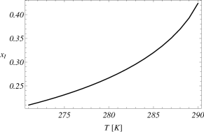
In the PNIPAM case (Cai and Suo,, 2011), we have that (4) is satisfied for $291.198$ K$<T<301.868$ K while (4.21) is never satisfied. This means that the system can exhibit (depending on the pressure) two coexisting phases for $T<T_{\textrm{low}}<291.198$ K and $T>T_{\textrm{high}}>301.868$ K. We recall that the numerical estimate for $T_{\textrm{low}}$ and $T_{\textrm{high}}$ are sharper and sharper provided $N_{x}$ is larger and larger.

This behavior is illustrated in in the first three panels of figure 3. The Maxwell construction is illustrated at $T=283$ K and $T=311$ K in order to find the value of the coexisting pressure, namely, the pressure such that the two gray areas in figure 3, or analogously the two local minima of the energy, are equal. Conversely at $T=300$ K the energy has a single minimum, for any value of the pressure, so that a unique phase is observed.

If the model b of the Flory interaction parameter is assumed, condition (3.18) yields

$$\begin{array}[]{l}[-1+2A_{0}-2A_{1}+(-1+A_{0}+2A_{1})^{2}]T^{2}\vphantom{\Big{\{}}\\ \phantom{mmmmmmmmm}+2B_{0}(A_{0}+2A_{1})T+B_{0}^{2}<0\end{array}$$ (4.22)

whereas conditions (3.19) read

$$\left\{\begin{array}[]{l}[-1+2A_{0}-2A_{1}+(-1+A_{0}+2A_{1})^{2}]T^{2}\\ \phantom{mmmmmmmm}+2B_{0}(A_{0}+2A_{1})T+B_{0}^{2}>0\\ -B_{0}+(1-A_{0}-2A_{1})T>0\\ -2B_{0}+(1-2A_{0}+2A_{1})T>0\\ \end{array}\right.$$ (4.23)

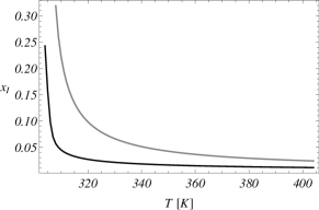
We have that (4.22) is satisfied for $126.869$ K$<T<303.825$ K while (4.23) is satisfied for $T<126.869$ K. This means that the system can exhibit (depending on the pressure) two coexisting phases for $T>T_{\textrm{high}}>303.825$ K. This behavior is illustrated in figure 3 (fourth panel). In the graph the Maxwell construction is illustrated at $T=315$ K and the coexistence pressure is found.

We remark that the estimate for the $T_{\textrm{high}}$ coexistence temperature is very similar in the two theories. The main difference is in the fact that with the model a phase coexistence is possible even at low temperature ($T<T_{\textrm{low}}$), while with the model b coexistence is possible only at high temperatures.

Figure 4: Coexistence pressures vs. temperature. Top: results for the model a at $T<T_{\textrm{low}}$ are plotted. Bottom: results for the model a (black) and for the model b (gray) at $T>T_{\textrm{high}}$ are plotted.

In the following we discuss the physical properties of the system in presence of two coexisting phases, the shrunk and the swollen one, which are the admissible equilibria with lower and higher volume change.

Figure 5: Coexisting phases vs. temperature. Top: results for the model a at $T<T_{\textrm{low}}$ are plotted. Bottom: results for the model a (black) and for the model b (gray) at $T>T_{\textrm{high}}$ are plotted.

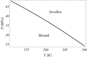
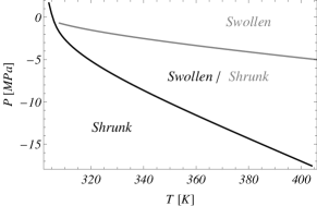
In figure 4 we plot the coexistence pressure versus the temperature. On the top we consider the model a at $T<T_{\textrm{low}}$ and note that the coexistence between the two phases occurs under compression. To the best of our knowledge the possibility of attaining coexistence in such regime has never been discussed in the related literature. On the bottom we consider both model a and model b at $T>T_{\textrm{high}}$, where we stress that the two models differ in the value of $T_{\textrm{high}}$ (see the discussion below (4.21) and (4.23)). The coexistence between the two phases occurs here under tension for almost all the considered values of temperature, but for the model a at temperatures close to $T_{\textrm{high}}$, where coexistence occurs under compression. It is worth to notice that in the $T$–$P$ plane there exist a region, the one between the two curves, where the two models predict different phases for the system.

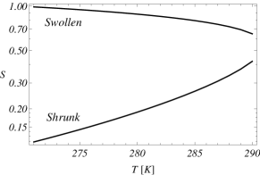
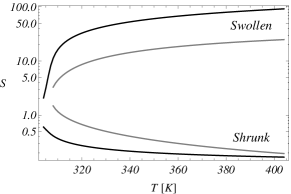
In figure 5 we plot the coexisting phases versus the temperature. On the top, we consider the model a at $T<T_{\textrm{low}}$ and, on the bottom, both model a and model b at $T>T_{\textrm{high}}$. It is worth to notice that the volume changes associated to the shrunk and the swollen phase are quite similar when $T<T_{\textrm{low}}$, while they significantly differ one from the other at $T>T_{\textrm{high}}$. Increasing the absolute difference between the current and the limit temperature, either $T_{\textrm{low}}$ or $T_{\textrm{high}}$, the shrunk and the swollen phase tend to separate from each other.

5 Interface location

Gradient theories are suitable to be developed for modeling stress/strain concentration due, for instance, to the presence of geometrical singularities (crack propagation in fracture mechanics) or phase transitions as in the case of wetting. To the best of our knowledge, gradient theories have rarely been formulated to infer interface location when temperature–driven volume transition occurs in hydrogels. Some recent results within the framework of phase–field models have been obtained in Hong and Wang, (2013).

Within the one–dimensional framework introduced above, the gradient theory will be used as a tool to capture the position of the interface between two coexisting phases differing in the degree of swelling (shrunk and swollen phases).

We consider the finite interval $[0,1]$ and introduce the Landau energy functional

$$\mathcal{F}[S]=\int_{0}^{1}\left[G(S)+\frac{\kappa}{2}(S^{\prime})^{2}\right]\mathrm{d}x$$ (5.24)

with the standard free–energy component $G(S)$, defined as in the equation (3.11), and $\kappa>0$ an appropriate higher order stiffness; the prime denotes the derivative with respect to the space variable. We look for the equilibrium profile $S(x)$ by performing a standard variational computation and assuming either Dirichlet or homogeneous Neumann boundary conditions. We therefore get the following Euler–Lagrange equation

$$\kappa S^{\prime\prime}=\frac{\partial G}{\partial S}.$$ (5.25)

We consider now Dirichlet boundary conditions corresponding to the shrunk ($S_{\mathrm{sh}}$) and the swollen ($S_{\mathrm{sw}}$) phases for the values of $P$ and $T$ ensuring coexistence. In other words, we solve the problem (5.25) with the boundary conditions

$$S(0)=S_{\mathrm{sh}}\;\;\textrm{ and }\;\;S(1)=S_{\mathrm{sw}}\;\;.$$ (5.26)

By exploiting the one–dimensionality of the model a phase space analysis proves that the problem (5.25) endowed with the above mentioned boundary conditions has a unique solution implicitly given by the integral

$$\int_{S_{\mathrm{sh}}}^{S}\frac{\sqrt{\kappa}\,\mathrm{d}s}{\sqrt{2[E_{\kappa}+G(s)]}}=x$$ (5.27)

where for any $\kappa>0$ we have defined implicitly $E_{\kappa}$ by the equation

$$\int_{S_{\mathrm{sh}}}^{S_{\mathrm{sw}}}\frac{\sqrt{\kappa}\,\mathrm{d}s}{\sqrt{2[E_{\kappa}+G(s)]}}=1$$ (5.28)

namely, the integral in (5.27) with $S=S_{\mathrm{sw}}$ and $x=1$.

The profile given by (5.27) is a connection between the two phases and, in the limit $\kappa\rightarrow 0$, presents a flat interface localized at

$$x_{I}=\frac{\sqrt{\partial^{2}G(S_{\mathrm{sw}})/\partial S^{2}}}{\sqrt{\partial^{2}G(S_{\mathrm{sh}})/\partial S^{2}}+\sqrt{\partial^{2}G(S_{\mathrm{sw}})/\partial S^{2}}}$$ (5.29)

see (Theorem 2) in (Cirillo et al.,, 2012). We note that, if the energy $G$ had equal second derivatives at the phases, the interface would fall in the middle point of the interval. We underline that in our case the energy (2.1) is not symmetric and therefore the interface position will change depending on the temperature $T$.

Figure 6: Profile (5.29) for the model a with $T=283$ K and $P=33.79$ MPa (left), and $T=308$ K and $P=-1.78$ MPa (center). Profile (5.29) for the model b with $T=308$ K and $P=-0.70$ MPa (right).

Figure 7: Interface position (5.29) as a function of temperature at coexisting pressure. On the left results for the model a at $T<T_{\textrm{low}}$ are plotted. On the right results for the model a (black) and for the model b (gray) at $T>T_{\textrm{high}}$ are plotted.

In figure 6, we show that the interface tends to a sharp kink when the stiffness is chosen smaller and smaller. We introduce a physically more relevant parameter, the characteristic length $\ell$ defined as

$$\ell^{2}=\frac{\Omega}{RT}\kappa\,.$$ (5.30)

We plot the solution of the equation (5.25) with Dirichlet boundary conditions (5.26) for different values of the characteristic length $\ell$ at given temperature and pressure ensuring coexistence. The plots show that the interface tends to localize in the small stiffness limit. In figure 6 (left and central panel) we solved the problem for the model a, whereas in figure 6 (right panel) the model b was considered. We remark that the boundary value problem (5.25)–(5.26) has been numerically solved by means of a properly implemented finite element code.

It is worth noting that, as already remarked above, due to the fact that even at coexistence the energy $G$ is not symmetric with respect to the central local maximum the position of the interface depends on the temperature. From the physical point of view, this means that at different temperatures the relative portions of the sample occupied by the shrunk and the swollen phases change.

It is interesting to compare the center and right panels in figure 6. At temperature $T=308$ K, the model a predicts that the interface position is close to the boundary where the shrunk phase is preserved; this means that the sample is mostly occupied by the swollen phase. On the other hand, at the same temperature, the model b predictions are slightly different, indeed the interface position is close to $0.3$ so that a not negligible part of the system is occupied by the shrunk phase.

In figure 7 the interface position is plotted as a function of the temperature for both models. The difference between the predictions of model a and model b is pointed out in the picture on the right. From both pictures we conclude that at temperatures far from the limiting values $T_{\textrm{low}}$ and $T_{\textrm{high}}$ the interface position is close to zero so that the sample is mostly occupied by the swollen phase. Conversely, the interface moves towards the center of the sample when the temperature gets closer to its limiting values. This effect is much more important for the model b.

We remark that our result goes in the opposite direction with respect to that illustrated in (Cai and Suo,, 2011, Fig. 14d). There, indeed, it is stated that at large temperature the shrunk phase tends to fill up the whole sample. However, we have to notice that the problems considered in our paper and in (Cai and Suo,, 2011) are similar, but not equivalent, indeed, the setup in that paper is fully three–dimensional, whereas our discussion is limited to dimension one.

6 Conclusions

We addressed the modeling of thermally–driven volume transition in hydrogels, within the Flory–Rehner thermodynamic setting; precisely, accounting for the temperature–depending pattern of the interaction parameter determined in (Hirotsu and Onuki,, 1989) for NIPA hydrogels, and in (Afroze et al.,, 2000) for aqueous solutions of uncrosslinked PNIPAM. In both models, the Flory parameter depends linearly on the volume fraction of polymer within the gel; on the contrary, the dependence on temperature is different. We proposed a detailed analysis aimed to establish the ranges of both temperature and traction which allow for the coexistence of two different phases (swollen and shrunk) in the hydrogel. With specific reference to a one–dimensional problem, we showed as different models for the interaction parameter deliver different conclusions.

Finally, for the values of temperature and traction ensuring phase coexistence, we presented a gradient model, appropriately extending the Flory–Rehner energy, and localize the interface position between the shrunk and the swollen phase, on one hand by means of a phase space analysis, previously developed by some of the Authors, on the other developing proper finite element numerical calculations.

References

- Tanaka et al., (1978) T. Tanaka, 1978. Physical Review Letters 40(12), 820–823.
- Tanaka et al., (1980) T. Tanaka, D. Fillmore, S. Sun, I. Nishio, G. Swislow, and A. Shah, 1980. Physical Review Letters 45(20), 1636–1639.
- Tanaka et al., (1984) Y. Hirokawa, T. Tanaka, 1984. J.Chem.Phys. 81(12), 6379–6380.
- Hirotsu, (1987) S. Hitotsu, 1987. Journal of the Physical Society of Japan 56(1), 233–242.
- Hirotsu and Onuki, (1989) S. Hirotsu and A. Onuki, 1989. Journal of the Physical Society of Japan 58(5), 1508–1511.
- Suzuki and Kojima, (1994) A. Suzuki and S. Kojima, 1994. J. Chem. Phys. 101, 10003.
- Suzuki et al., (1997) A. Suzuki, K. Sanda, Y. Omori, 1997. J. Chem. Phys. 107(13), 5179–5185.
- Doi, (2009) M. Doi, 2009. Journal of the Physical Society of Japan 78(5), 052001.
- Birgesson et al., (2008) E. Birgersson, H. Li, S. Wu, 2008. Journal of the Mechanics and Physics of Solids 56, 444- 466.
- Cai and Suo, (2011) S. Cai, A. Suo, 2011. Journal of the Mechanics and Physics of Solids 59, 2259–2278.
- Chester and Anand, (2011) S.A. Chester and L. Anand, 2011. Journal of the Mechanics and Physics of Solids 59, 1978–2006.
- Ding et al., (2013) Z. Ding, Z. Liu, J. Hu, S. Swaddiwudhipong, Z. Yang, 2013. International Journal of Solids and Structures 50, 2610 -2619
- Drozdov, (2014) A.D. Drozdov, 2014. The European Physical Journal E 37, 93.
- Drozdov and Sommer–Larsen, (2015) A.D. Drozdov and P. Sommer–Larsen, 2015. Swelling of thermo-responsive gels under hydrostatic pressure Meccanica, Published on line: 9 October 2015.
- Duda et al., (2010) F.P. Duda, A.C. Souza, E. Fried, 2010. Journal of the Mechanics and Physics of Solids 58, 515–529.
- Hong and Wang, (2013) W. Hong and X. Wang, 2013. Journal of the Mechanics and Physics Solids 61, 1281–1294.
- Ji et al., (2006) H. Ji, H. Mourad, E. Fried, J. Dolbow, 2006. International Journal of Solids and Structures 43, 1878- 1907.
- Afroze et al., (2000) F. Afroze, E. Nies, H. Berghmans, 2000. Journal of Molecular Structure 554, 55 -68.
- Cirillo et al., (2012) E.N.M. Cirillo, N. Ianiro, and G. Sciarra, 2012. Physical Review E 86, 041111.
- Lucantonio et al., (2013) A. Lucantonio, P. Nardinocchi, L. Teresi, 2013. Journal of the Mechanics and Physics of Solids 61, 205 -218.
- Rubinstein, (2003) M. Rubinstein and R.H. Colby, 2003. Polymer Physics. Oxford University Press.
- Doi, (1996) M. Doi, 1996. Introduction to Polymer Physics. Clarendon Press, Oxford.
- Cirillo et al., (2009) E.N.M. Cirillo, N. Ianiro, and G. Sciarra, 2009. Solid–fluid segregation in saturated porous media. Poromechanics IV: Proceedings of the Fourth BIOT Conference on Poromechanics, DEStech Publications, Inc.
- Cirillo et al., (2010) E.N.M. Cirillo, N. Ianiro, and G. Sciarra, 2010. Phase coexistence in consolidating porous media. Physical Review E 81, 061121–1–9.
- Cirillo et al., (2011) E.N.M. Cirillo, N. Ianiro, and G. Sciarra, 2011. Phase transition in saturated porous–media: pore–fluid segregation in consolidation. Physica D 240, 1345–1351.
- Cirillo et al., (2013) E.N.M. Cirillo, N. Ianiro, and G. Sciarra, 2013. Journal of the Mechanics and Physics of Solids 61, 1080–1114.