Reconstruction in the Labeled Stochastic Block Model

Abstract

The labeled stochastic block model is a random graph model representing networks with community structure and interactions of multiple types. In its simplest form, it consists of two communities of approximately equal size, and the edges are drawn and labeled at random with probability depending on whether their two endpoints belong to the same community or not.

It has been conjectured in [16] that correlated reconstruction (i.e. identification of a partition correlated with the true partition into the underlying communities) would be feasible if and only if a model parameter exceeds a threshold. We prove one half of this conjecture, i.e., reconstruction is impossible when below the threshold. In the positive direction, we introduce a weighted graph to exploit the label information. With a suitable choice of weight function, we show that when above the threshold by a specific constant, reconstruction is achieved by (1) minimum bisection, (2) a semidefinite relaxation of minimum bisection, and (3) a spectral method combined with removal of edges incident to vertices of high degree. Furthermore, we show that hypothesis testing between the labeled stochastic block model and the labeled Erdős-Rényi random graph model exhibits a phase transition at the conjectured reconstruction threshold.

1 Introduction

1.1 Motivation

Community detection aims to identify underlying communities of similar characteristics in an overall population from the observation of pairwise interactions between individuals [12, 24, 23]. The stochastic block model, also known as planted partition model, is a popular random graph model for analyzing the community detection problem [25, 28, 2, 27, 9], in which pairwise interactions are binary: an edge is either present or absent between two individuals. In its simplest form, the stochastic block model consists of two communities of approximately equal size, where the within-community edge is present at random with probability $p$; while the across-community edge is present with probability $q$. If $p>q$, it corresponds to assortative communities where interactions are more likely within rather than across communities; while $p<q$ corresponds to disassortative communities.

In practice, interactions can be of various types and these types reveal more information on the underlying communities than the mere existence of the interaction itself. For example, in recommender systems, interactions between users and items come with user ratings. Such ratings contain far more information than the interaction itself to characterize the user and item types. Similarly, protein-protein chemical interactions in biological networks can be exothermic and endothermic; email exchanges in a club may be formal or informal; friendship in social networks may be strong or weak. The labeled stochastic block model was recently proposed in [16] to capture rich interaction types. In this model interaction types are described by labels drawn from an arbitrary collection. In particular, for the simple two communities case, the within-community edge is labeled at random with distribution $\mu$; while the across-community edge is labeled with a different distribution $\nu$. In this context an important question is how to leverage the labeling information for detecting underlying communities.

1.2 Information-Scarce Regime

In this paper, we focus on the sparse labeled stochastic block model in which every vertex has a limited average degree, i.e., $p,q=O(1/n)$, where $n$ is the number of vertices. It corresponds to the information-scarce regime where only $O(n)$ edges and labels are observed in total. This regime is of practical interest, arising in several contexts. For example, in recommender systems, users only give ratings to few items; in biological networks, only few protein-protein interactions are observed due to cost constraints; in social networks, a person only has a limited number of friends.

For the stochastic block model in this information-scarce regime, there are $\Theta(n)$ isolated vertices, as in Erdős-Rényi random graphs with bounded average degree. For isolated vertices, it is impossible to determine their community membership and thus exact reconstruction of communities is impossible. Therefore, we resort to finding a partition into communities positively correlated to the true community partition (see Definition 1 below).

1.3 Main Results

Focusing on the two communities scenario, we show that a positively correlated reconstruction is fundamentally impossible when below a threshold. This establishes one half of the conjecture in [16]. In the positive direction, we establish the following results. We introduce a graph weighted by a suitable function of observed labels, on which we show that:

(1) Minimum bisection gives a positively correlated partition when above the threshold by a factor of $64\ln 2$.

(2) A semidefinite relaxation of minimum bisection gives a positively correlated partition when above the threshold by a factor of $2^{17}\ln 2$.

(3) A spectral method combined with removal of edges incident to vertices of high degree gives a positively correlated partition when above the threshold by a constant factor.

Furthermore, we show that the labeled stochastic block model is contiguous to a labeled Erdős-Rényi random graph when below the reconstruction threshold and orthogonal to it when above the threshold. It implies that for the hypothesis testing problem between the labeled stochastic block model and the labeled Erdős-Rényi random graph model, the correct identification of the underlying distribution is feasible if and only if above the reconstruction threshold. It also implies that there is no consistent estimator for model parameters when below the reconstruction threshold.

1.4 Related Work

For the stochastic block model, most previous work focuses on the “dense” regime with an average degree diverging as the size of the graph $n$ grows, (see, e.g., [4, 5] and the references therein). For the “sparse” regime with bounded average degrees, a sharp phase transition threshold for reconstruction was conjectured in [9] by analyzing the belief propagation algorithm. The converse part of the conjecture was rigorously proved in [22]. The achievability part is proved independently in [21, 19]. In addition, it is shown in [6] that a variant of spectral method gives a positively correlated partition when above the threshold by an unknown constant factor. More recently, it is shown in [15] that a semidefinite program finds a correlated partition when above the threshold by some large constant factor.

The labeled stochastic block was first proposed and studied in [16] and a new reconstruction threshold that incorporates the extra labeling information was conjectured. Simulations further indicate that the belief propagation algorithm works when above the threshold, but reconstruction algorithms that provably work are still unknown.

Finally, we recently became aware of the work [1] that studies the problem of decoding binary node labels from noisy edge measurements. In the case where the background graph is Erdős-Rényi random graph and each node label is independently and uniformly chosen from $\{\pm 1\}$, the model in [1] can be viewed as a special case of the labeled stochastic block model with $p=q$, $\mu=(1-\epsilon)\delta_{+1}+\epsilon\delta_{-1}$ and $\nu=\epsilon\delta_{+1}+(1-\epsilon)\delta_{-1}$, where $\delta_{x}$ denotes the probability measure concentrated on point $x$ (See Section 2 for the formal model description). When $p=q=a\log n/n$ for some constant $a$ and $\epsilon\to 1/2$, it is shown in [1] that exact recovery of node labels is possible if and only if $a(1-2\epsilon)^{2}>2$. In contrast, our results show that when $p=q=a/n$ for some constant $a$, correlated recovery of node labels is impossible if $a(1-2\epsilon)^{2}<1$ for any $0\leq\epsilon\leq 1$. Moreover, we show that distinguishing hypothesis $\epsilon=\epsilon_{0}$ and hypothesis $\epsilon=1/2$ is possible if and only if $a(1-2\epsilon_{0})^{2}>1$.

1.5 Outline

Section 2 introduces the precise definition of the labeled stochastic block model to be studied and the key notations. The main theorems are introduced and briefly discussed in Section 3. The detailed proofs are presented in Section 4. Section 5 ends the paper with concluding remarks. Miscellaneous details and proofs are in the Appendix.

2 Model and Notation

This section formally defines the labeled stochastic block model with two symmetric communities and introduces the key notations and definitions used in the paper. Let $\mathcal{L}$ denote a finite set. The labeled stochastic block model $\mathcal{G}(n,p,q,\mu,\nu)$ is a random graph with $n$ vertices of $\{\pm 1\}$ types indexed by $[n]$ and $\{\ell\in\mathcal{L}\}$-labeled edges. To generate a particular realization $(G,L,\sigma)$, first assign type $\sigma_{u}\in\{\pm 1\}$ to each vertex $u$ uniformly and independently at random. Then, for every vertex pair $(u,v)$, independently of everything else, draw an edge between $u$ and $v$ with probability $p$ if $\sigma_{u}=\sigma_{v}$ and with probability $q$ otherwise. Finally, every edge $e=(u,v)$ is labeled with $\ell$ independently at random with probability $\mu(\ell)$ if $\sigma_{u}=\sigma_{v}$ and with probability $\nu(\ell)$ otherwise.

Equivalently, we can specify $\mathcal{G}(n,p,q,\mu,\nu)$ by its probability distribution. Let

$$\phi_{uv}(G,L,\sigma)=\left\{\begin{array}[]{rl}p\mu(L_{uv})&\text{if }\sigma_{u}=\sigma_{v},(u,v)\in E(G),\\ q\nu(L_{uv})&\text{if }\sigma_{u}\neq\sigma_{v},(u,v)\in E(G),\\ 1-p&\text{if }\sigma_{u}=\sigma_{v},(u,v)\notin E(G),\\ 1-q&\text{if }\sigma_{u}\neq\sigma_{v},(u,v)\notin E(G),\end{array}\right.$$

where $E(G)$ is the set of edges of $G$ and $L_{uv}$ is the label on the edge $(u,v)$. Then,

$$\mathbb{P}_{n}(G,L,\sigma)=2^{-n}\prod_{(u,v):u<v}\phi_{uv}(G,L,\sigma).$$ (4)

When $\mu=\nu$, it reduces to the classical stochastic block model without labels. This paper focuses on the sparse case where $p=a/n$ and $q=b/n$ for two fixed constants $a$ and $b$, and the goal is to reconstruct the true underlying types of vertices $\sigma$ by observing the graph structure $G$ and the labels on edges $L$.

It is known that in the sparse graph, there are $\Theta(n)$ isolated vertices whose types clearly cannot be recovered accurately. Therefore, our goal is to reconstruct a type assignment which is positively correlated to the true type assignment. More formally, we adopt the following definition.

Definition 1.

A type assignment $\widehat{\sigma}$ is said to be positively correlated with the true type assignment $\sigma$ if a.a.s.

$$\ Q(\sigma,\widehat{\sigma}):=\frac{1}{2}-\frac{1}{n}\min\{d(\sigma,\widehat{\sigma}),d(\sigma,-\widehat{\sigma})\}>0,$$ (5)

where $d$ is the Hamming distance, and $Q$ is called the Overlap.

The shorthand a.a.s. denotes asymptotically almost surely. A sequence of events $A_{n}$ holds a.a.s. if the probability of $A_{n}$ converges to $1$ as $n\to\infty$. Define $\tau$ as

$$\tau=\frac{a+b}{2}\sum_{\ell\in\mathcal{L}}\frac{a\mu(\ell)+b\nu(\ell)}{a+b}\left(\frac{a\mu(\ell)-b\nu(\ell)}{a\mu(\ell)+b\nu(\ell)}\right)^{2}.$$ (6)

It was conjectured in [16] that $\tau$ is the threshold for positively correlated reconstruction.

Conjecture 1.

• If $\tau>1$, then it is possible to find a type assignment correlated with the true assignement a.a.s.

• If $\tau<1$, then it is impossible to find a type assignment correlated with the true assignement a.a.s.

In this paper, we prove (ii) and propose three different algorithms able to find a type assignment correlated with the true assignment for $\tau$ big enough.

Notation

Let $A$ denote the adjacency matrix of the graph $G$, $\mathbf{I}$ denote the identity matrix, and $\mathbf{J}$ denote the all-one matrix. We write $X\succeq 0$ if $X$ is positive semidefinite and $X\geq 0$ if all the entries of $X$ are non-negative. For any matrix $Y$, let $\|Y\|$ denote its spectral norm. For any positive integer $n$, let $[n]=\{1,\ldots,n\}$. For any set $T\subset[n]$, let $|T|$ denote its cardinality and $T^{c}$ denote its complement. We use standard big $O$ notations, e.g., for any sequences $\{a_{n}\}$ and $\{b_{n}\}$, $a_{n}=\Theta(b_{n})$ or $a_{n}\asymp b_{n}$ if there is an absolute constant $c>0$ such that $1/c\leq a_{n}/b_{n}\leq c$. Let ${\rm Bern}(p)$ denote the Bernoulli distribution with mean $p$ and ${\rm Binom}(N,p)$ denote the binomial distribution with $N$ trials and success probability $p$. All logarithms are natural and we use the convention $0\log 0=0$. For a vector $x\in{\mathbb{R}}^{n}$, $\mathsf{sign}(x)$ gives the sign of $x$ componentwise, and $\|x\|$ denotes the $L_{2}$ norm. For a graph $G$, let $V(G)$ denote its vertex set and $E(G)$ denote its edge set.

3 Main Theorems

3.1 Minimum Bisection

To recover the community partition, one approach is via the maximum likelihood estimation. In view of (4), the log-likelihood function can be written as:

$$\log\mathbb{P}(G,L|\sigma) = \frac{1}{2}\sum_{(u,v)\in E(G)}\left[\log\frac{a\mu(L_{uv})}{b\nu(L_{uv})}\sigma_{u}\sigma_{v}+\log\left(\frac{ab}{n^{2}}\mu(L_{uv})\nu(L_{uv})\right)\right]$$

$$+ \frac{1}{2}\sum_{(u,v)\notin E(G)}\left[\log\left(\frac{1-a/n}{1-b/n}\right)\sigma_{u}\sigma_{v}+\log\left((1-a/n)(1-b/n)\right)\right].$$

Under the constraint $\sum_{u}\sigma_{u}=0$, the maximum likelihood estimation is equivalent to

$$\max_{\sigma}\quad \sum_{(u,v)\in E(G)}\log\left[\frac{a(1-b/n)\mu(L_{uv})}{b(1-a/n)\nu(L_{uv})}\right]A_{uv}\sigma_{u}\sigma_{v}$$

s.t. $$\sum_{u}\sigma_{u}=0,\;\sigma\in\{\pm 1\}^{n}.$$

This is equivalent to the minimum bisection on the weighted graph with a specific weight function $w(\ell)=\log\frac{a(1-b/n)\mu(\ell)}{b(1-a/n)\nu(\ell)}$. For a general weighing function $w:\mathcal{L}\to[-1,1]$, the minimum bisection finds a balanced bipartite subgraph in $G$ with the minimum weighted cut, i.e.,

$$\min_{\sigma} \sum_{(u,v):\sigma_{u}\neq\sigma_{v}}W_{uv}$$

s.t. $$\sum_{u}\sigma_{u}=0,\;\sigma_{u}\in\{\pm 1\},$$ (7)

where $W_{uv}=A_{uv}w(L_{uv})$ and $A$ is the adjacency matrix of $G$.

Theorem 1.

Assume the technical condition: $\sum_{\ell}a\mu(\ell)w^{2}(\ell),\sum_{\ell}b\nu(\ell)w^{2}(\ell)>8\ln 2$. Then if

$$\frac{\sum_{\ell}(a\mu(\ell)-b\nu(\ell))w(\ell)}{\sqrt{\sum_{\ell}(a\mu(\ell)+b\nu(\ell))w^{2}(\ell)}}>\sqrt{128\ln 2},$$ (8)

a.a.s. solutions of the minimum bisection (7) are positively correlated to the true type assignment $\sigma^{\ast}.$ Moreover, the left hand side of (8) is maximized when $w(\ell)=\frac{a\mu(\ell)-b\nu(\ell)}{a\mu(\ell)+b\nu(\ell)}$, in which case (8) reduces to $\tau>64\ln 2$.

3.2 Semidefinite relaxation method

The minimum bisection is known to be NP-hard in the worst case [14, Theorem 1.3]. In this section, we present a semidefinite relaxation of the minimum bisection (7) which is solvable in polynomial time, and show it finds an assignment correlated with the true assignment provided $\tau$ is large enough. Let $Y=\sigma\sigma^{\top}$. Then $\sigma_{u}=\pm 1$ is equivalent to $Y_{uu}=1$, and $\sum_{u}\sigma_{u}=0$ if and only if $\langle Y,\mathbf{J}\rangle=0$. Therefore, (7) can be recast as

$$\max_{Y,\sigma} \;\langle W,Y\rangle$$

s.t. $$\;Y=\sigma\sigma^{\top}$$

$$\;Y_{uu}=1,\quad u\in[n]$$

$$\;\langle\mathbf{J},Y\rangle=0.$$ (9)

Notice that the matrix $Y=\sigma\sigma^{\top}$ is a rank-one positive semidefinite matrix. If we relax this condition by dropping the rank-one restriction, we obtain the following semidefinite relaxation of (9):

$$\widehat{Y}_{{\rm SDP}}=\mathop{\arg\max}_{Y} \;\langle W,Y\rangle$$

s.t. $$\;Y\succeq 0$$

$$\;Y_{uu}=1,\quad u\in[n]$$

$$\;\langle\mathbf{J},Y\rangle=0.$$ (10)

To get an estimator of the type assignment from $\widehat{Y}_{{\rm SDP}}$, let $y$ denote an eigenvector of $\widehat{Y}_{{\rm SDP}}$ corresponding to the largest eigenvalue and $\|y\|=\sqrt{n}$. The following result shows that $\widehat{\sigma}_{{\rm SDP}}\triangleq\mathsf{sign}(y)$ is positively correlated with the true type assignment.

Theorem 2.

Assume the technical condition: $\sum_{\ell}w^{2}(\ell)(a\mu(\ell)+b\nu(\ell))>8\ln 2$. If

$$\frac{\sum_{\ell}(a\mu(\ell)-b\nu(\ell))w(\ell)}{\sqrt{\sum_{\ell}(a\mu(\ell)+b\nu(\ell))w^{2}(\ell)}}>512\sqrt{\ln 2},$$ (11)

then a.a.s. $\widehat{\sigma}_{{\rm SDP}}$ is positively correlated to the true type assignment $\sigma^{\ast}$. Moreover, the left hand side of (11) is maximized when $w(\ell)=\frac{a\mu(\ell)-b\nu(\ell)}{a\mu(\ell)+b\nu(\ell)}$, in which case (11) reduces to $\tau>2^{17}\ln 2$.

In the stochastic block model without labels, i.e., $\mu=\nu$, condition (11) reduces to $(a-b)^{2}>2^{18}\ln 2(a+b)$; similar conditions with a different constant have been proved in [15, Theorem 1.1] using the Grothendieck’s inequality. Our proof builds upon the analysis in [15].

3.3 Spectral Method

In this section, we present a polynomial-time spectral algorithm based on the weighted adjacency matrix $W$ and show that this algorithm allows us to find an assignment correlated with the true assignment provided $\tau$ is large enough.

Note that $\mathbb{E}[W|\sigma]=\frac{\alpha}{n}\mathbf{J}+\frac{\beta}{n}\sigma\sigma^{\top}-\frac{\alpha+\beta}{n}\mathbf{I}$ with

$$\alpha=\frac{1}{2}\sum_{\ell}w(\ell)(a\mu(\ell)+b\nu(\ell)),$$

$$\beta=\frac{1}{2}\sum_{\ell}w(\ell)(a\mu(\ell)-b\nu(\ell)).$$ (12)

The term $\frac{\alpha+\beta}{n}\mathbf{I}$ is irrelevant to the main results (thanks to Weyl’s perturbation theorem) and neglected for simplicity. Let $D=W-\frac{\alpha}{n}\mathbf{J}$ and then $\mathbb{E}[D|\sigma]=\frac{\beta}{n}\sigma\sigma^{\top}$ has rank one with singular value $\beta$. Hence, it makes sense to define $\widehat{D}$ as the best rank-1 approximation of the matrix $D$. In other words, if $D=\sum_{i}v_{i}x_{i}x_{i}^{\top}$ is the eigenvalue decomposition of $D$ with eigenvalues $|v_{1}|\geq|v_{2}|\geq\dots$, we define $\widehat{D}=v_{1}x_{1}x_{1}^{\top}$. Then if the matrix $D$ is close to its mean $\mathbb{E}[D|\sigma]$ in the spectral norm, we expect $v_{1}$ to be close to $\beta$, and $\mathsf{sign}(x_{1})$ to be correlated with $\sigma$. Unfortunately, in the sparse regime, there are vertices of degree $\Omega(\frac{\log n}{\log\log n})$ and thus the largest singular value of $W$ could reach $\Omega(\sqrt{\frac{\log n}{\log\log n}})$ which is much higher than $\beta$. In order to take care of the issue, we begin with a preliminary step to clean the spectrum of $W$: we remove all edges incident to vertices in the graph with degree larger than $\frac{3}{2}\frac{a+b}{2}$. To summarize, for a given weight function $w(\ell)$, our algorithm $\rm{Spectral-Reconstruction}$ has the following structure:

1. Remove edges incident to vertices with degree larger than $\frac{3}{2}\frac{a+b}{2}$ and let $G^{\prime}$ denote the resulting graph. Define $W^{\prime}$ to be the weighted adjacency matrix of $G^{\prime}$.

2. Let $\widehat{x}$ be the left-singular vector associated with the largest singular value of $D^{\prime}=W^{\prime}-\frac{\alpha}{n}\mathbf{J}$, i.e.,

   $$\widehat{x}=\arg\max\{|x^{\top}D^{\prime}x|,\>\|x\|=1\}.$$ (13)

   Output ${\rm sign}(\widehat{x})$ for the types of the vertices.

Observe that (13) can be seen as a (non-convex) relaxation of the minimum bisection (7) by replacing the integer constraint with the unit-norm constraint and relaxing the constraint $\sum_{u}\sigma_{u}=0$ to be a regularized term $\frac{\alpha}{n}x^{\top}\mathbf{J}x$ in the objective function. $\rm{Spectral-Reconstruction}$ needs estimates of $\alpha$ and $a+b$, which can be well approximated by $\frac{1}{n}\mathbf{1}^{\top}W\mathbf{1}$ and $\frac{2}{n}\mathbf{1}^{\top}A\mathbf{1}$, respectively. To simplify the analysis, we will assume that the exact values of $\alpha$ and $a+b$ are known.

Theorem 3.

Assume $a>b>C_{0}$ for some sufficiently large constant $C_{0}$. There exists a universal constant $C$ (i.e. not depending on $a$, $b$, $\mu$ or $\nu$) such that if $\beta^{2}>C(a+b)$, where $\beta$ is defined in (12), then a.a.s. $\rm{Spectral-Reconstruction}$ outputs a type assignment correlated with the true assignment. In the particular case, where $w(\ell)=\frac{a\mu(\ell)-b\nu(\ell)}{a\mu(\ell)+b\nu(\ell)}$, the condition $\beta^{2}>C(a+b)$ reduces to $\tau>\sqrt{C(a+b)}$.

In the stochastic block model without labels, letting $w(\ell)=1$, condition $\beta^{2}>C(a+b)$ reduces to $(a-b)^{2}>4C(a+b)$; the sharp condition $(a-b)^{2}>2(a+b)$ has been proved recently in [21, 19]. Compared to point (i) in the Conjecture 1, our result does not give the right order of magnitude when $a$ and $b$ are large. Indeed, we are able to improve it if we allow $a$ and $b$ to grow with $n$.

Theorem 4.

Assume that $\min(a,b)=\Omega(\log^{6}n)$. If

$$\frac{[\sum_{\ell}(a\mu(\ell)-b\nu(\ell))w(\ell)]^{2}}{\sum_{\ell}(a\mu(\ell)+b\nu(\ell))w^{2}(\ell)}>256,$$ (14)

then $\rm{Spectral-Reconstruction}$ outputs a type assignment correlated with the true assignment a.a.s. Moreover, the left hand side of (14) is maximized when $w(\ell)=\frac{a\mu(\ell)-b\nu(\ell)}{a\mu(\ell)+b\nu(\ell)}$, in which case (14) reduces to $\tau>128$. With this choice of $w(\ell)$, as soon as $\tau\to\infty$, $\rm{Spectral-Reconstruction}$ outputs the true assignment for all vertices except $o(n)$ a.a.s.

Note that in the regime $\min(a,b)=\Omega(\log^{6}n)$, the degrees are very concentrated and step 1) of the algorithm can be removed without harm. The simulation results, depicted in Fig. 1, further indicate that $\rm{Spectral-Reconstruction}$ leaving out step 1) outputs a positively correlated assignment when above the threshold. In the simulation, we assume for simplicity only two labels: $r$ and $b$, and define $\mu(r)=0.5+\epsilon$ and $\nu(r)=0.5-\epsilon$. We generate the graph from the labeled stochastic block model with $n=1000$ vertices for various $a,b,\epsilon$. Fix $a,b$, we plot the overlap $Q$ against $\epsilon$ and indicate the threshold $\tau=1$ as a vertical dash line. All plotted values are averages over $100$ trials.

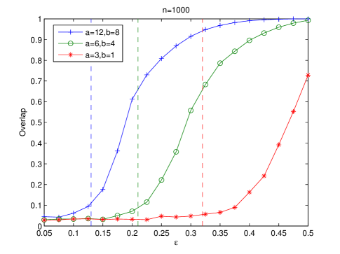
Figure 1: The overlap $Q$ against $\epsilon$ from $0.05$ to $0.5$.

Note that our algorithm is most efficient when the parameters ($a$, $b$, $\mu$ and $\nu$) of the model are known as the optimal weight function depends on these parameters. In the case where the labels are uninformative, i.e. $\mu=\nu$, our algorithm is very simple, does not require to know the values $a$ and $b$, and in the range of Theorem 4, has the best known performance guarantee (see [4, Table I]).

3.4 Converse Result

This section proves part (ii) of Conjecture 1. In particular, we show that when $\tau<1$, asymptotically it is impossible to tell whether any two vertices are more likely to belong to the same community. It further implies that reconstructing a positively correlated type assignment is fundamentally impossible.

Theorem 5.

If $\tau<1$, then for any fixed vertices $\rho$ and $v$,

$$\mathbb{P}_{n}(\sigma_{\rho}=+1|G,L,\sigma_{v}=+1)\to 1/2\text{ a.a.s}.$$ (15)

Remark 1.

Reconstructing a positively correlated type assignment is harder than telling whether any two vertices are more likely to belong to the same community. In particular, given a positively correlated type assignment $\widehat{\sigma}$, for two vertices randomly chosen, they are more likely to belong to the same community if they have the same type in $\widehat{\sigma}$.

Theorem 5 is related to the Ising spin model in the statistical physics [10, 20], and it essentially says that there is no long range correlation in the type assignment when $\tau<1$. The main idea in the proof of Theorem 5 is borrowed from [22] and works as follows: (1) pick any two fixed vertices $\rho,v$ and consider the local neighborhood of $\rho$ up to distance $O(\log(n))$. The vertex $v$ lies outside of the local neighborhood of $\rho$ a.a.s.. (2) conditional on the type assignment at the boundary of the local neighborhood, $\sigma_{\rho}$ is asymptotically independent with $\sigma_{v}$. (3) the local neighborhood of $\rho$ looks like a Markov process on a labeled Galton-Watson tree rooted at $\rho$. (4) For the Markov process on the labeled Galton-Watson tree, the types of leaves provide no information about the type of the root $\rho$ when the depth of tree goes to infinity.

3.5 Hypothesis Testing

Consider a labeled Erdős-Rényi random graph $\mathcal{G}(n,\frac{a+b}{2})$, where independently at random, each pair of two vertices is connected with probability $\frac{a+b}{2}$, and every edge is labeled with $\ell\in\mathcal{L}$ with probability $\frac{a\mu(\ell)+b\nu(\ell)}{a+b}.$ Let $\mathbb{P}^{\prime}_{n}$ denote the distribution of the labeled Erdős-Rényi random graph.

Given a graph $(G,L)$ which was drawn from either $\mathbb{P}_{n}$ or $\mathbb{P}^{\prime}_{n}$, an interesting hypothesis testing problem is to decide which one is the underlying distribution of $(G,L)$? It turns out that when $\tau>1$, the correct identification of the underlying distribution is feasible a.a.s.; however, when $\tau<1$, one is bound to make error with non-vanishing probability.

Theorem 6.

If $\tau>1$, then $\mathbb{P}_{n}$ and $\mathbb{P}^{\prime}_{n}$ are asymptotically orthogonal, i.e., there exists event $A_{n}$ such that $\mathbb{P}_{n}(A_{n})\to 1$ and $\mathbb{P}^{\prime}_{n}(A_{n})\to 0$.

If $\tau<1$, then $\mathbb{P}_{n}$ and $\mathbb{P}^{\prime}_{n}$ are contiguous, i.e., for every sequence of event $A_{n}$,

$$\lim_{n\to\infty}\mathbb{P}_{n}(A_{n})=0\Leftrightarrow\lim_{n\to\infty}\mathbb{P}_{n}^{\prime}(A_{n})=0.$$

Theorem 6 further implies the following corollary regarding the model parameter estimation.

Corollary 1.

If $\tau<1$, then there is no consistent estimator for parameters $a,b,\mu,\nu$.

Proof.

The second part of Theorem 6 implies that $\mathcal{G}(n,\frac{a_{1}}{n},\frac{b_{1}}{n},\mu_{1},\nu_{1})$ and $\mathcal{G}(n,\frac{a_{2}}{n},\frac{b_{2}}{n},\mu_{2},\nu_{2})$ are contiguous as long as $a_{1}\mu_{1}(\ell)+b_{1}\nu_{1}(\ell)=a_{2}\mu_{2}(\ell)+b_{2}\nu_{2}(\ell)$ and

$$\sum_{\ell}\frac{(a_{i}\mu_{i}(\ell)-b_{i}\nu_{i}(\ell))^{2}}{2(a_{i}\mu_{i}(\ell)+b_{i}\nu_{i}(\ell))}<1,$$

for $i=1,2$. Therefore, one cannot distinguish between $\mathcal{G}(n,\frac{a_{1}}{n},\frac{b_{1}}{n},\mu_{1},\nu_{1})$ and $\mathcal{G}(n,\frac{a_{2}}{n},\frac{b_{2}}{n},\mu_{2},\nu_{2})$ with the success probability converging to $1$, and thus there is no consistent estimator for parameters $a,b,\mu,\nu$. ∎

In the special case where $\mu=\nu$, i.e., no labeling information is available, Theorem 6 reduces to Theorem 2.4 in [22]. The positive part of Theorem 6 is proved by counting the number of labeled short cycles and the second moment method. The negative part of Theorem 6 is proved using the small subgraph conditioning method as introduced in [22]. The small subgraph conditioning method was originally developed to show that random $d$-regular graphs are Hamiltonian a.s.s. [26, 17].

4 Proofs

4.1 Proof of Theorem 1

Recall that $\sigma^{\ast}$ denotes the true type assignment. Since $|\{u:\sigma^{\ast}_{u}=1\}|\sim{\rm Binom}(n,1/2)$, by Chernoff bound, a.a.s.,

$$|\{u:\sigma^{\ast}_{u}=1\}|\in\left[n/2-\sqrt{n\log n},n/2+\sqrt{n\log n}\right].$$ (16)

For ease of presentation, assume $|\{u:\sigma^{\ast}_{u}=1\}|=n/2$. Let $m(\sigma)\triangleq|\{u:\sigma_{u}=+1,\sigma^{\ast}_{u}=-1\}|$ and $\epsilon>0$ be an arbitrarily small constant. To prove the theorem, by the definition of positively correlated reconstruction, it suffices to show that for all $\sigma$ with $\frac{n}{4}(1-\epsilon)\leq m(\sigma)\leq\frac{n}{4}$,

$$\sum_{\begin{subarray}{c}(u,v):\sigma_{u}\neq\sigma_{v},\\ \sigma_{u}^{\ast}=\sigma_{v}^{\ast}\end{subarray}}W_{uv}-\sum_{\begin{subarray}{c}(u,v):\sigma_{u}=\sigma_{v},\\ \sigma_{u}^{\ast}\neq\sigma_{v}^{\ast}\end{subarray}}W_{uv}:=Y_{1}(\sigma)-Y_{2}(\sigma)>0.$$

To ease the notation, we suppress the argument $\sigma$. Observe that $Y_{1}$ is a sum of $2m(n/2-m)$ i.i.d. random variables whose value is $w(\ell)$ with probability $\frac{a}{n}\mu(\ell)$; $Y_{2}$ is a sum of $2m(n/2-m)$ i.i.d. random variables whose value is $w(\ell)$ with probability $\frac{b}{n}\nu(\ell)$. Thus,

$$y_{1} :=\mathbb{E}[Y_{1}]=2m(n/2-m)(a/n)\sum_{\ell}\mu(\ell)w(\ell),$$

$$y_{2} :=\mathbb{E}[Y_{2}]=2m(n/2-m)(b/n)\sum_{\ell}\nu(\ell)w(\ell).$$

Define

$$z_{1} :=2m(n/2-m)(a/n)\sum_{\ell}\mu(\ell)w^{2}(\ell),$$

$$z_{2} :=2m(n/2-m)(b/n)\sum_{\ell}\nu(\ell)w^{2}(\ell).$$

Then, for $0<\lambda\leq\frac{1}{2}$,

$$\mathbb{E}[\exp(-\lambda Y_{1})] =\left[1+\frac{a}{n}\sum_{\ell}({\rm e}^{-\lambda w(\ell)}-1)\mu(\ell)\right]^{2m(n/2-m)}$$

$$\leq\exp\left[2m(n/2-m)\frac{a}{n}\sum_{\ell}({\rm e}^{-\lambda w(\ell)}-1)\mu(\ell)\right]$$

$$\leq\exp\left[2m(n/2-m)\frac{a}{n}\sum_{\ell}\left(-\lambda w(\ell)+2\lambda^{2}w^{2}(\ell)\right)\mu(\ell)\right]$$

$$=\exp(-\lambda y_{1}+2\lambda^{2}z_{1}),$$

where the first inequality follows from the fact that $1+x\leq e^{x}$ and the second one follows from the fact that $e^{x}\leq 1+x+2x^{2}$ for $|x|\leq 1/2$. The Chernoff bound gives that for $0<\lambda\leq\frac{1}{2}$,

$$\mathbb{P}(Y_{1}\leq(1-t)y_{1}) \leq\mathbb{E}[\exp(-\lambda Y_{1})]\exp((1-t)\lambda y_{1})$$

$$\leq\exp(-t\lambda y_{1}+2\lambda^{2}z_{1}).$$ (17)

We define $\mathbb{E}[W_{\mu}]\triangleq\sum_{\ell}\mu(\ell)w(\ell)$ and $\mathbb{E}[W_{\mu}^{2}]\triangleq\sum_{\ell}\mu(\ell)w^{2}(\ell)$. Let $t_{1}^{2}=(64\ln 2)\frac{1+\epsilon}{1-\epsilon}\frac{1}{a}\frac{\mathbb{E}[W_{\mu}^{2}]}{\left(\mathbb{E}[W_{\mu}]\right)^{2}}$ and $\lambda=\frac{t_{1}y_{1}}{4z_{1}}$. We first check that with these values, we have $\lambda\leq 1/2$:

$$\lambda\leq\frac{1}{2} \Leftrightarrow t_{1}\leq\frac{2\mathbb{E}[W_{\mu}^{2}]}{\mathbb{E}[W_{\mu}]}$$

$$\Leftrightarrow \frac{1+\epsilon}{1-\epsilon}\frac{8\ln 2}{a}\leq\mathbb{E}[W^{2}_{\mu}].$$

Thanks to the assumption made in Theorem 1, we can find $\epsilon$ sufficiently small such that this last inequlity is valid. Notice that $\frac{t_{1}^{2}y_{1}^{2}}{8z_{1}}\geq(1+\epsilon)^{2}n\ln 2.$ It follows from (17) that

$$\mathbb{P}(Y_{1}\leq(1-t_{1})y_{1})=\exp\left(-\frac{t_{1}^{2}y_{1}^{2}}{8z_{1}}\right)\leq 2^{-n(1+\epsilon)}.$$

Since there are $\binom{n/2}{m}\binom{n/2}{m}\leq 2^{n}$ different $\sigma$ with $m(\sigma)=m$, a simple union bound yields that as $n\to\infty$,

$$\mathbb{P}\left(\exists\sigma:(1-\epsilon)n/4\leq m(\sigma)\leq n/4,Y_{1}\leq(1-t_{1})y_{1}\right)\to 0.$$

Similarly, let $t_{2}^{2}=(64\ln 2)\frac{1+\epsilon}{1-\epsilon}\frac{1}{b}\frac{\mathbb{E}[W_{\nu}^{2}]}{\left(\mathbb{E}[W_{\nu}]\right)^{2}}$ with $\mathbb{E}[W_{\nu}]\triangleq\sum_{\ell}\nu(\ell)w(\ell)$ and $\mathbb{E}[W_{\nu}^{2}]\triangleq\sum_{\ell}\nu(\ell)w^{2}(\ell)$. Then

$$\mathbb{P}\left(\exists\sigma:(1-\epsilon)n/4\leq m(\sigma)\leq n/4,Y_{2}\geq(1+t_{2})y_{2}\right)\to 0.$$

With $\epsilon$ sufficiently small, a.a.s.

$$Y_{1}-Y_{2} \geq(1-t_{1})y_{1}-(1+t_{2})y_{2}$$

$$=y_{1}-y_{2}-\frac{2m}{n}(n/2-m)\sqrt{\frac{1+\epsilon}{1-\epsilon}(64\ln 2)}\left(\sqrt{a\mathbb{E}[W_{\mu}^{2}]}+\sqrt{b\mathbb{E}[W_{\nu}^{2}]}\right)$$

$$\geq\frac{2m}{n}(n/2-m)\left(a\mathbb{E}[W_{\mu}]-b\mathbb{E}[W_{\nu}]-\sqrt{\frac{1+\epsilon}{1-\epsilon}(128\ln 2)}\sqrt{\left(a\mathbb{E}[W_{\mu}^{2}]+b\mathbb{E}[W_{\nu}^{2}]\right)}\right)$$

which is larger than zero as soon as $\epsilon$ is sufficiently small and (8) is satisfied.

By Cauchy-Schwartz inequality,

$$\left(\sum_{\ell}(a\mu(\ell)-b\nu(\ell))w(\ell)\right)^{2}\leq 2\tau\sum_{\ell}(a\mu(\ell)+b\nu(\ell))w^{2}(\ell)$$

with equality achieved when $w(\ell)=\frac{a\mu(\ell)-b\nu(\ell)}{a\mu(\ell)+b\nu(\ell)}$. This completes the proof.

4.2 Proof of Theorem 2

Without loss of generality, assume (16) holds for $\sigma^{\ast}$. Let $Y^{\ast}=\sigma^{\ast}(\sigma^{\ast})^{\top}$. By the optimality of $\widehat{Y}_{{\rm SDP}}$,

$$0\leq\langle W,\widehat{Y}_{{\rm SDP}}\rangle-\langle W,Y^{\ast}\rangle=\langle\mathbb{E}[W],\widehat{Y}_{{\rm SDP}}-Y^{\ast}\rangle+\langle W-\mathbb{E}[W],\widehat{Y}_{{\rm SDP}}-Y^{\ast}\rangle.$$ (18)

Since $\mathbb{E}[W]=\frac{\alpha}{n}\mathbf{J}+\frac{\beta}{n}Y^{\ast}-\frac{\alpha+\beta}{n}\mathbf{I}$ with $\alpha,\beta$ defined in (12), and $\widehat{Y}_{{\rm SDP}}$ is a feasible solution to (9),

$$\langle\mathbb{E}[W],\widehat{Y}_{{\rm SDP}}-Y^{\ast}\rangle=\frac{\beta}{n}\langle Y^{\ast},\widehat{Y}_{{\rm SDP}}-Y^{\ast}\rangle-\frac{\alpha}{n}\langle\mathbf{J},Y^{\ast}\rangle\leq\frac{\beta}{n}\langle Y^{\ast},\widehat{Y}_{{\rm SDP}}-Y^{\ast}\rangle,$$

where the last inequality holds because $\langle\mathbf{J},Y^{\ast}\rangle\geq 0$. In view of (18), it follows that

$$\frac{\beta}{n}\langle Y^{\ast},Y^{\ast}-\widehat{Y}_{{\rm SDP}}\rangle\leq\langle W-\mathbb{E}[W],\widehat{Y}_{{\rm SDP}}-Y^{\ast}\rangle.$$ (19)

Notice that

$$\|Y^{\ast}-\widehat{Y}_{{\rm SDP}}\|_{\rm F}^{2}=\|Y^{\ast}\|_{\rm F}^{2}+\|\widehat{Y}_{{\rm SDP}}\|_{\rm F}^{2}-2\langle Y^{\ast},\widehat{Y}_{{\rm SDP}}\rangle\leq 2\left(n^{2}-\langle Y^{\ast},\widehat{Y}_{{\rm SDP}}\rangle\right)=2\langle Y^{\ast},Y^{\ast}-\widehat{Y}_{{\rm SDP}}\rangle.$$

It follows from (19) that

$$\frac{\beta}{2n}\|Y^{\ast}-\widehat{Y}_{{\rm SDP}}\|_{\rm F}^{2}\leq\langle W-\mathbb{E}[W],\widehat{Y}_{{\rm SDP}}-Y^{\ast}\rangle\leq|\langle W-\mathbb{E}[W],\widehat{Y}_{{\rm SDP}}\rangle|+|\langle W-\mathbb{E}[W],Y^{\ast}\rangle|.$$ (20)

To upper bound $|\langle W-\mathbb{E}[W],Y^{\ast}\rangle|$, Notice that

$$\langle W-\mathbb{E}[W],Y^{\ast}\rangle=2\sum_{i<j}Y^{\ast}_{ij}\left(W_{ij}-\mathbb{E}[W_{ij}]\right).$$

Let $\sigma^{2}=\sum_{i<j}\mathsf{var}[W_{ij}]=(1+o(1))\frac{n}{2}\sum_{\ell}w^{2}(\ell)(a\mu(\ell)+b\nu(\ell)).$ By the Bernstein inequality given in Theorem 8, for any $t>0$,

$$\mathbb{P}\left\{\bigg{|}\sum_{i<j}Y^{\ast}_{ij}\left(W_{ij}-\mathbb{E}[W_{ij}]\right)\bigg{|}\geq\sqrt{2\sigma^{2}t}+\frac{2}{3}t\right\}\leq 2{\rm e}^{-t}.$$

Letting $t=\log n=o(\sigma^{2})$, it follows that with probability at least $1-2n^{-1}$,

$$\big{|}\sum_{i<j}Y^{\ast}_{ij}\left(W_{ij}-\mathbb{E}[W_{ij}]\right)\big{|}\leq(1+o(1))\sqrt{n\log n\sum_{\ell}w^{2}(\ell)(a\mu(\ell)+b\nu(\ell))},$$

and thus $|\langle W-\mathbb{E}[W],Y^{\ast}\rangle|\leq(2+o(1))\sqrt{n\log n\sum_{\ell}w^{2}(\ell)(a\mu(\ell)+b\nu(\ell))}$ with probability at least $1-2n^{-1}$.

We bound $|\langle W-\mathbb{E}[W],\widehat{Y}_{{\rm SDP}}\rangle|$ next. It follows from Grothendieck’s inequality [15, Theorem 3.4] that

$$|\langle W-\mathbb{E}[W],\widehat{Y}_{{\rm SDP}}\rangle|\leq\sup_{Y\succeq 0,\mathsf{diag}\left\{{Y}\right\}=\mathbf{I}}|\langle W-\mathbb{E}[W],Y\rangle|\leq K_{\rm G}\|W-\mathbb{E}[W]\|_{\infty\to 1},$$

where $K_{\rm G}$ is an absolute constant known as Grothendieck constant and it is known that $K_{\rm G}<\frac{\pi}{2\ln(1+\sqrt{2})}\leq 1.783$. Moreover,

$$\|W-\mathbb{E}[W]\|_{\infty\to 1}\triangleq\sup_{x:\|x\|_{\infty}\leq 1}\|(W-\mathbb{E}[W])x\|_{1} =\sup_{x,y\in\{\pm 1\}^{n}}x^{\top}(W-\mathbb{E}[W])y$$

$$=\sup_{x,y\in\{\pm 1\}^{n}}\sum_{i<j}\left(W_{ij}-\mathbb{E}[W_{ij}]\right)(x_{i}y_{j}+x_{j}y_{i}).$$

For any fixed $x,y\in\{\pm 1\}^{n}$, using the Bernstein inequality, we have for any $t>0$,

$$\mathbb{P}\left\{\sum_{i<j}\left(W_{ij}-\mathbb{E}[W_{ij}]\right)(x_{i}y_{j}+x_{j}y_{i})\geq\sqrt{8\sigma^{2}t}+\frac{4}{3}t\right\}\leq{\rm e}^{-t}.$$

Hence, for arbitrarily small constant $\epsilon>0$, with probability at least $2^{-2(1+\epsilon)n}$,

$$\sum_{i<j}\left(W_{ij}-\mathbb{E}[W_{ij}]\right)(x_{i}y_{j}+x_{j}y_{i}) \leq n\left(\sqrt{8\ln 2(1+\epsilon)\sum_{\ell}w^{2}(\ell)(a\mu(\ell)+b\nu(\ell))}+\frac{8\ln 2(1+\epsilon)}{3}\right)$$

$$\overset{(a)}{\leq}\frac{4n}{3}\sqrt{8\ln 2(1+\epsilon)\sum_{\ell}w^{2}(\ell)(a\mu(\ell)+b\nu(\ell))},$$

where $(a)$ follows from the technical assumption $\sum_{\ell}w^{2}(\ell)(a\mu(\ell)+b\nu(\ell))>8\ln 2$. It follows from the union bound that with probability at least $1-4^{-\epsilon n}$,

$$\|W-\mathbb{E}[W]\|_{\infty\to 1}\leq\frac{4n}{3}\sqrt{8\ln 2(1+\epsilon)\sum_{\ell}w^{2}(\ell)(a\mu(\ell)+b\nu(\ell))}.$$

In view of (20), with probability at least $1-4^{-\epsilon n}-2n^{-1}$,

$$\frac{1}{n^{2}}\|Y^{\ast}-\widehat{Y}_{{\rm SDP}}\|_{\rm F}^{2} \leq(1+o(1))\frac{8K_{\rm G}}{3\beta}\sqrt{8\ln 2(1+\epsilon)\sum_{\ell}w^{2}(\ell)(a\mu(\ell)+b\nu(\ell))}$$

$$\overset{(a)}{\leq}(1+o(1))32\sqrt{\ln 2(1+\epsilon)}\frac{\sqrt{\sum_{\ell}w^{2}(\ell)(a\mu(\ell)+b\nu(\ell))}}{\sum_{\ell}w(\ell)(a\mu(\ell)-b\nu(\ell)}$$

$$\overset{(b)}{\leq}(1-\epsilon)\frac{1}{16},$$ (21)

where $(a)$ follows by $\sqrt{2}K_{G}\leq 3$ and the definition of $\beta$ given in (12); $(b)$ holds by invoking (11) and letting $\epsilon$ be sufficiently small.

Recall that $y$ is an eigenvector of $\widehat{Y}_{{\rm SDP}}$ corresponding to the largest eigenvalue and $\|y\|=\sqrt{n}$. By Davis-Kahan sin$\theta$ theorem stated in Lemma 5,

$$\frac{1}{\sqrt{n}}\min\{\|\sigma^{\ast}-y\|,\|\sigma^{\ast}+y\|\}\leq\frac{2\sqrt{2}\|\widehat{Y}_{{\rm SDP}}-Y^{\ast}\|}{n}\leq\frac{2\sqrt{2}\|\widehat{Y}_{{\rm SDP}}-Y^{\ast}\|_{\rm F}}{n}.$$

Note that for any $x\in\mathbb{R}^{n}$, Hamming distance $d(\sigma^{\ast},\mathsf{sign}(x))\leq\|\sigma^{\ast}-x\|^{2}.$ It follows that

$$\frac{1}{n}\min\{d(\sigma^{\ast},\mathsf{sign}(y)),d(\sigma^{\ast},\mathsf{sign}(-y))\}\leq\frac{8\|\widehat{Y}_{{\rm SDP}}-Y^{\ast}\|_{\rm F}}{n^{2}},$$

and the theorem holds in view of (21).

4.3 Proof of Theorem 3

Recall that $W^{\prime}$ is the weighted adjacency matrix after removal of edges incident to vertices with high degrees and $D^{\prime}=W^{\prime}-\frac{\alpha}{n}\mathbf{J}$. Define $\widehat{D^{\prime}}$ as the best rank-1 approximation of $D^{\prime}$ such that $\widehat{D^{\prime}}=v_{1}xx^{\top}$ with $\|x\|=1$. Recall that $\mathbb{E}[D|\sigma]=\frac{\beta}{n}\sigma\sigma^{\top}$. Applying Davis-Kahan $\sin\theta$ theorem restated in Lemma 5 with $D^{\prime}$ and $\mathbb{E}[D|\sigma]$ gives:

$$\min\{\|\frac{\sigma}{\sqrt{n}}-x\|,\|\frac{\sigma}{\sqrt{n}}+x\|\}\leq\frac{2\sqrt{2}}{|\beta|}\|D^{\prime}-\mathbb{E}[D|\sigma]\|.$$

Since Hamming distance $d(\sigma,\mathsf{sign}(x)\leq\|\sigma-\sqrt{n}x\|^{2}$, it follows that

$$\frac{1}{n}\min\{d(\sigma,\mathsf{sign}(x),d(\sigma,-\mathsf{sign}(x))\}\leq\frac{8}{\beta^{2}}\|D^{\prime}-\mathbb{E}[D|\sigma]\|^{2}=\frac{8}{\beta^{2}}\|W^{\prime}-\mathbb{E}[W|\sigma]\|^{2}.$$ (22)

Lemma 6 implies that a.a.s. $\|W^{\prime}-\mathbb{E}[W|\sigma]\|\leq C\sqrt{a+b}$ for some universal positive constant $C$. Hence, in view of (22), we get

$$\frac{1}{n}\min\{d(\sigma,\mathsf{sign}(\widehat{x}),d(\sigma,-\mathsf{sign}(\widehat{x}))\}\leq 8C^{2}\frac{a+b}{\beta^{2}},$$

and the theorem follows.

4.4 Proof of Theorem 4

The proof follows the same steps as for Theorem 3, except that we are able to strengthen Lemma 6 thanks to a result of Vu [30]. Note that the variance of the elements of $W$ is upper bounded by $\frac{1}{n}\sum_{\ell}w^{2}(\ell)\left(a\mu(\ell)+b\nu(\ell)\right)$ so that by Theorem 1.4 in [30], we get

Lemma 1.

Under the conditions of Theorem 4, we have

$$\|W-\mathbb{E}[W|\sigma]\|\leq 2\sqrt{\sum_{\ell}w^{2}(\ell)\left(a\mu(\ell)+b\nu(\ell)\right)}\quad a.a.s.$$

4.5 Proof of Theorem 5

Consider a Galton-Watson tree $T$ with Poisson offspring distribution with mean $\frac{a+b}{2}$. The type of the root $\rho$ is chosen from $\{\pm 1\}$ uniformly at random. Each child has the same type as its parent with probability $\frac{a}{a+b}$ and a different type with probability $\frac{b}{a+b}$ . Every edge $(u,v)$ is labeled at random with distribution $\mu$ if $\sigma_{u}=\sigma_{v}$ and $\nu$ otherwise. Let $T_{R}$ denote the Galton-Watson tree $T$ up to depth $R$ and $\partial T_{R}$ denote the set of leaves of $T_{R}$. Let $G_{R}$ denote the subgraph of $G$ induced by vertices up to distance $R$ from $\rho$ and $\partial G_{R}$ be the set of vertices at distance $R$ from $\rho$.

The following lemma similar to Proposition 4.2 in [22] establishes a coupling between the local neighborhood of $\rho$ and the labeled Galton-Watson tree rooted at $\rho$.

Lemma 2.

Let $R=R(n)=\lfloor\frac{\log n}{10\log(2(a+b))}\rfloor$, then there exists a coupling such that a.a.s.

$$(G_{R},L_{G_{R}},\sigma_{G_{R}})=(T_{R},L_{T_{R}},\sigma_{T_{R}}),$$

where $L_{G_{R}}$ and $\sigma_{G_{R}}$ denote the labels and types on the subgraph $G_{R}$, respectively.

Proof.

See proof in Section C. ∎

To ease notation, we omit the shorthand a.a.s. in the sequel. To prove Theorem 5, it suffices to show that $\text{Var}(\sigma_{\rho}|G,L,\sigma_{v})\to 1$. By the law of total variance,

$$\text{Var}(\sigma_{\rho}|G,L,\sigma_{v})=\mathbb{E}_{\sigma_{\partial G_{R}}}\left[\text{Var}(\sigma_{\rho}|G,L,\sigma_{v},\sigma_{\partial G_{R}})\right]+\text{Var}_{\sigma_{\partial G_{R}}}\left[\mathbb{E}\left[\sigma_{\rho}|G,L,\sigma_{v},\sigma_{\partial G_{R}}\right]\right].$$

Hence, it further reduces to show that $\text{Var}(\sigma_{\rho}|G,L,\sigma_{v},\sigma_{\partial G_{R}})\to 1$.

Let $R$ be as in Lemma 2, then $G_{R}=o(\sqrt{n})$ and thus $v\notin G_{R}$. Lemma 4.7 in [22] shows that $\sigma_{\rho}$ is asymptotically independent with $\sigma_{v}$ conditionally on $\sigma_{\partial G_{R}}$. Hence,

$$\text{Var}(\sigma_{\rho}|G,L,\sigma_{v},\sigma_{\partial G_{R}})\to\text{Var}(\sigma_{\rho}|G,L,\sigma_{\partial G_{R}}).$$

Let $G_{R}^{c}$ denote the subgraph of $G$ induced by edges not in $G_{R}$, and $L_{G_{R}^{c}}$ denote the set of labels on $G_{R}^{c}$. Recall that $V(G_{R-1})$ and $V(G_{R}^{c})$ denote the set of vertices in $G_{R-1}$ and $G_{R}^{c}$, respectively. Let $S\triangleq V(G_{R-1})\setminus\{\rho\}$ and $T\triangleq V(G_{R}^{c})\setminus\partial G_{R}.$ Then $\{\rho\}\cup\partial G_{R}\cup S\cup T=V(G)$. Notice that conditional on $(G_{R},L_{G_{R}},\sigma_{\partial G_{R}})$, $\sigma_{\rho}$ is independent of $(G_{R}^{c},L_{G_{R}^{c}})$. In particular,

$$\mathbb{P}\left\{\sigma_{\rho}|G_{R},L_{G_{R}},\sigma_{\partial G_{R}}\right\}$$

$$=\frac{\sum_{G_{R}^{c},L_{G_{R}^{c}}}\mathbb{P}\left\{\sigma_{\rho},G,L,\sigma_{\partial G_{R}}\right\}}{\sum_{G_{R}^{c},L_{G_{R}^{c}}}\mathbb{P}\left\{G,L,\sigma_{\partial G_{R}}\right\}}$$

$$=\frac{\sum_{G_{R}^{c},L_{G_{R}^{c}}}\left(\sum_{\sigma_{S}}\prod_{u,v\in V(G_{R}):u<v}\phi_{uv}\right)\left(\sum_{\sigma_{T}}\prod_{u,v\in T:u<v}\phi_{uv}\prod_{u\in\partial G_{R},v\in T}\phi_{uv}\right)}{\sum_{G_{R}^{c},L_{G_{R}^{c}}}\left(\sum_{\sigma_{\rho}}\sum_{\sigma_{S}}\prod_{u,v\in V(G_{R}):u<v}\phi_{uv}\right)\left(\sum_{\sigma_{T}}\prod_{u,v\in T:u<v}\phi_{uv}\prod_{u\in\partial G_{R},v\in T}\phi_{uv}\right)}$$

$$\overset{(a)}{=}\frac{\left(\sum_{\sigma_{S}}\prod_{u,v\in V(G_{R}):u<v}\phi_{uv}\right)\sum_{G_{R}^{c},L_{G_{R}^{c}}}\left(\sum_{\sigma_{T}}\prod_{u,v\in T:u<v}\phi_{uv}\prod_{u\in\partial G_{R},v\in T}\phi_{uv}\right)}{\left(\sum_{\sigma_{\rho}}\sum_{\sigma_{S}}\prod_{u,v\in V(G_{R}):u<v}\phi_{uv}\right)\sum_{G_{R}^{c},L_{G_{R}^{c}}}\left(\sum_{\sigma_{T}}\prod_{u,v\in T:u<v}\phi_{uv}\prod_{u\in\partial G_{R},v\in T}\phi_{uv}\right)}$$

$$=\frac{\sum_{\sigma_{S}}\prod_{(u,v)\in V(G_{R}):u<v}\phi_{uv}}{\sum_{\sigma_{\rho}}\sum_{\sigma_{S}}\prod_{(u,v)\in G_{R}:u<v}\phi_{uv}}$$

$$=\frac{\left(\sum_{\sigma_{S}}\prod_{(u,v)\in V(G_{R}):u<v}\phi_{uv}\right)\left(\sum_{\sigma_{T}}\prod_{u,v\in T:u<v}\phi_{uv}\prod_{u\in\partial G_{R},v\in T}\phi_{uv}\right)}{\left(\sum_{\sigma_{\rho}}\sum_{\sigma_{S}}\prod_{(u,v)\in V(G_{R}):u<v}\phi_{uv}\right)\left(\sum_{\sigma_{T}}\prod_{u,v\in T:u<v}\phi_{uv}\prod_{u\in\partial G_{R},v\in T}\phi_{uv}\right)}$$

$$=\frac{\mathbb{P}\left\{\sigma_{\rho},G,L,\sigma_{\partial G_{R}}\right\}}{\mathbb{P}\left\{G,L,\sigma_{\partial G_{R}}\right\}}=\mathbb{P}\left\{\sigma_{\rho}|G,L,\sigma_{\partial G_{R}}\right\},$$

where $(a)$ holds because $\sum_{\sigma_{S}}\prod_{(u,v)\in V(G_{R}):u<v}\phi_{uv}$ does not depend on $G_{R}^{c}$ and $L_{G_{R}^{c}}$. It follows that

$$\text{Var}(\sigma_{\rho}|G,L,\sigma_{\partial G_{R}})=\text{Var}(\sigma_{\rho}|G_{R},L_{G_{R}},\sigma_{\partial G_{R}}).$$

Lemma 2 implies that

$$\text{Var}(\sigma_{\rho}|G_{R},L_{G_{R}},\sigma_{\partial G_{R}})\to\text{Var}(\sigma_{\rho}|T_{R},L_{T_{R}},\sigma_{\partial T_{R}}).$$

For the labeled Galton-Watson tree, it was shown in [16] that if $\tau<1$, the types of the leaves provide no information about the type of the root when the depth $R\to\infty$, i.e.,

$$\mathbb{P}(\sigma_{\rho}=+1|T,L,\sigma_{\partial T_{R}})\to\frac{1}{2}.$$

Hence, $\text{Var}(\sigma_{\rho}|T_{R},L_{T_{R}},\sigma_{\partial T_{R}})\to 1$ and the theorem follows.

4.6 Proof of Theorem 6

We introduce some necessary notations. For a graph $G$ with $n$ vertices and labeled edges, denote a $k$-sequence of labels by $[\ell]_{k}=(\ell_{1},\ell_{2},\ldots,\ell_{k})\in\mathcal{L}^{k}$. A cycle in $G$ is called a $k$-cycle with labels $[\ell]_{k}$, if starting from the vertex with the minimum index and ending at its neighbor with the smaller index among its two neighbors, the sequence of labels on edges is given by $[\ell]_{k}$. Let $X_{n}([\ell]_{k})$ denote the number of $k$-cycles with labels $[\ell]_{k}$ in $G$. Let $(X)_{j}=X(X-1)\cdots(X-j+1)$ for integers $X$ and $1\leq j\leq X$. Then $(X_{n}([\ell]_{k}))_{j}$ is the number of ordered $j$-tuples of $k$-cycles with labels $[\ell]_{k}$ in $G$. The product $\prod_{[\ell]_{k}}$ is assumed to taken over all possible sequences of labels with length $k$. The following lemma gives the asymptotic distribution of the number of $k$-cycles with labels $[\ell]_{k}$.

Lemma 3.

For any fixed integer $m\geq 3$, $\{X_{n}([\ell]_{k}):[\ell]_{k}\in{\mathcal{L}}^{k}\}_{k=3}^{m}$ jointly converge to independent Poisson random variables with mean $\lambda([\ell]_{k})$ under graph distribution $\mathbb{P}_{n}^{\prime}$, and $\xi([\ell]_{k})$ under graph distribution $\mathbb{P}_{n}$, where

$$\lambda([\ell]_{k})=\frac{1}{2^{k+1}k}\prod_{i=1}^{k}(a\mu(\ell_{i})+b\nu(\ell_{i})),$$

$$\xi([\ell]_{k})=\frac{1}{2^{k+1}k}\left(\prod_{i=1}^{k}(a\mu(\ell_{i})+b\nu(\ell_{i}))+\prod_{i=1}^{k}(a\mu(\ell_{i})-b\nu(\ell_{i}))\right).$$

We are ready to prove Theorem 6. The first part of Theorem 6 is proved using Lemma 3 and Chebyshev inequality. Define $\eta([\ell]_{k})=\xi([\ell]_{k})/\lambda([\ell]_{k})-1$ and $X_{k}=\sum_{[\ell]_{k}}X([\ell]_{k})\eta([\ell]_{k})$. Then, by Lemma 3, as $n\to\infty$,

$$\mathbb{E}_{\mathbb{P}^{\prime}}[X_{k}] =\sum_{[\ell]_{k}}\lambda([\ell]_{k})\eta([\ell]_{k}),$$

$$\mathbb{E}_{\mathbb{P}}[X_{k}] =\sum_{[\ell]_{k}}\lambda([\ell]_{k})\eta([\ell]_{k})(1+\eta([\ell]_{k})).$$

Note that

$$2k\sum_{[\ell]_{k}}\lambda([\ell]_{k})\eta^{2}([\ell]_{k})=\sum_{[\ell]_{k}}\prod_{s=1}^{k}\frac{(a\mu(\ell_{s})-b\nu(\ell_{s}))^{2}}{2(a\mu(\ell_{s})+b\nu(\ell_{s}))}=\left(\sum_{\ell\in\mathcal{L}}\frac{(a\mu(\ell)-b\nu(\ell))^{2}}{2(a\mu(\ell)+b\nu(\ell))}\right)^{k}=\tau^{k}.$$ (23)

Therefore,

$$\mathbb{E}_{\mathbb{P}}[X_{k}]-\mathbb{E}_{\mathbb{P}^{\prime}}[X_{k}]=\sum_{[\ell]_{k}}\lambda([\ell]_{k})\eta^{2}([\ell]_{k})=\tau^{k}/(2k),$$

and

$$\text{Var}_{\mathbb{P}^{\prime}}[X_{k}] =\sum_{[\ell]_{k}}\lambda([\ell]_{k})\eta^{2}([\ell]_{k})=\tau^{k}/(2k),$$

$$\text{Var}_{\mathbb{P}}[X_{k}] =\sum_{[\ell]_{k}}\xi([\ell]_{k})\eta^{2}([\ell]_{k})\leq\tau^{k}/k.$$

Choose $\rho=\tau^{k}/(6k)$. By Chebyshev’s inequality,

$$\mathbb{P}^{\prime}\{X_{k}>\mathbb{E}_{\mathbb{P}^{\prime}}[X_{k}]+\rho\}\leq\frac{\text{Var}_{\mathbb{P}^{\prime}}[X_{k}]}{\rho^{2}}=\frac{18k}{\tau^{k}}.$$

Let $k$ increases with $n$ sufficiently slowly. Then since $\tau>1$, $X_{k}\leq\mathbb{E}_{\mathbb{P}^{\prime}}[X_{k}]+\rho$ $\mathbb{P}^{\prime}$-a.a.s.. Similarly, $X_{k}\geq\mathbb{E}_{\mathbb{P}}[X_{k}]-\rho$ $\mathbb{P}$-a.a.s.. By definition of $\rho$, $\mathbb{E}_{\mathbb{P}}[X_{k}]-\rho>\mathbb{E}_{\mathbb{P}^{\prime}}[X_{k}]+\rho$. Set $A_{n}=\{X_{k}\leq\mathbb{E}_{\mathbb{P}^{\prime}}[X_{k}]+\rho\}$, then $\mathbb{P}^{\prime}(A_{n})\to 1$ and $\mathbb{P}(A_{n})\to 0$.

The second part of Theorem 6 is proved using the following small subgraph conditioning theorem, which is adapted from [17, Theorem 9.12].

Theorem 7.

Let $Y_{n}=\frac{\mathbb{P}_{n}}{\mathbb{P}_{n}^{\prime}}$. If $\mathbb{P}_{n}$ and $\mathbb{P}_{n}^{\prime}$ are absolutely contiguous for any fixed $n$, and

1. For each fixed $m\geq 3$, $\{X_{n}([\ell]_{k})\}_{k=3}^{m}$ converge jointly to independent Poisson variables with means $\lambda([\ell]_{k})>0$ under distribution $\mathbb{P}_{n}^{\prime}$, and $\xi([\ell]_{k})$ under distribution $\mathbb{P}_{n}$;

2. $\sum_{k\geq 3}\sum_{[\ell]_{k}}\lambda([\ell]_{k})\eta([\ell]_{k})^{2}<\infty$;

3. $\mathbb{E}_{\mathbb{P}^{\prime}_{n}}[Y_{n}^{2}]\to\exp(\sum_{k\geq 3}\sum_{[\ell]_{k}}\lambda([\ell]_{k})\eta^{2}([\ell]_{k}))$ as $n\to\infty$,

Then, $\mathbb{P}_{n}$ and $\mathbb{P}_{n}^{\prime}$ are contiguous.

In this paper, $\mathbb{P}_{n}$ and $\mathbb{P}_{n}^{\prime}$ are discrete distributions on the space of labeled graphs, and for any fixed $n$, $\mathbb{P}_{n}$ and $\mathbb{P}_{n}^{\prime}$ are absolutely continuous. Condition 1) is verified by Lemma 3. Condition 2) holds because in view of (23),

$$\sum_{k\geq 3}\sum_{[\ell]_{k}}\lambda([\ell]_{k})\eta^{2}([\ell]_{k})=\sum_{k\geq 3}\frac{\tau^{k}}{2k}=-\frac{\log(1-\tau)+\tau+\tau^{2}/2}{2}<\infty.$$ (24)

We are left to verify condition 3). By definition,

$$Y_{n}(G,L)=2^{-n}\sum_{\sigma\in\{\pm 1\}^{n}}\prod_{(u,v):u<v}W_{u,v}(G,L,\sigma),$$

where

$$W_{uv}(G,L,\sigma)=\left\{\begin{array}[]{rl}\frac{2a\mu(l)}{a\mu(\ell)+b\nu(\ell)}&\text{if }\sigma_{u}=\sigma_{v},(u,v)\in E(G),L_{uv}=\ell,\\ \frac{2b\nu(l)}{a\mu(\ell)+b\nu(\ell)}&\text{if }\sigma_{u}\neq\sigma_{v},(u,v)\in E(G),L_{uv}=\ell,\\ \frac{1-a/n}{1-(a+b)/(2n)}&\text{if }\sigma_{u}=\sigma_{v},(u,v)\notin E(G),\\ \frac{1-b/n}{1-(a+b)/(2n)}&\text{if }\sigma_{u}\neq\sigma_{v},(u,v)\notin E(G),\end{array}\right.$$ (29)

Then,

$$Y_{n}^{2}=2^{-2n}\sum_{\sigma,\delta\in\{\pm 1\}^{n}}\prod_{(u,v):u<v}W_{u,v}(G,L,\sigma)W_{u,v}(G,L,\delta).$$ (30)

Lemma 4.

For any fixed $\sigma,\delta\in\{\pm 1\}^{n}$, if $\sigma_{u}\sigma_{v}=\delta_{u}\delta_{v}$, then

$$\mathbb{E}_{\mathbb{P}^{\prime}_{n}}[W_{u,v}(G,L,\sigma)W_{u,v}(G,L,\delta)]=1+\tau/n+(a-b)^{2}/(4n^{2})+O(n^{-3}).$$

Otherwise,

$$\mathbb{E}_{\mathbb{P}^{\prime}_{n}}[W_{u,v}(G,L,\sigma)W_{u,v}(G,L,\delta)]=1-\tau/n-(a-b)^{2}/(4n^{2})+O(n^{-3}).$$

Proof.

Suppose $\sigma_{u}\sigma_{v}=\delta_{u}\delta_{v}=1$. Then,

$$\mathbb{E}_{\mathbb{P}^{\prime}_{n}}[W_{u,v}(G,L,\sigma)W_{u,v}(G,L,\delta)]$$

$$=\sum_{\ell}\left(\frac{2a\mu(\ell)}{a\mu(\ell)+b\nu(\ell)}\right)^{2}\frac{a\mu(\ell)+b\nu(\ell)}{2n}+\left(\frac{1-a/n}{1-(a+b)/(2n)}\right)^{2}\left(1-\frac{a+b}{2n}\right)$$

$$=\frac{1}{n}\sum_{\ell}\frac{2a^{2}\mu^{2}(\ell)}{a\mu(\ell)+b\nu(\ell)}+\left(1-\frac{a}{n}\right)^{2}\left(1+\frac{a+b}{2n}+\frac{(a+b)^{2}}{4n^{2}}+O(n^{-3})\right)$$

$$=1+\frac{1}{n}\sum_{\ell}\left(\frac{2a^{2}\mu^{2}(\ell)}{a\mu(\ell)+b\nu(\ell)}+\frac{b\nu(\ell)-3a\mu(\ell)}{2}\right)+\frac{(a-b)^{2}}{4n^{2}}+O(n^{-3})$$

$$=1+\frac{1}{n}\sum_{\ell}\frac{(a\mu(\ell)-b\nu(\ell))^{2}}{2(a\mu(\ell)+b\nu(\ell))}+\frac{(a-b)^{2}}{4n^{2}}+O(n^{-3})$$

$$=1+\tau/n+(a-b)^{2}/(4n^{2})+O(n^{-3}).$$ (31)

By symmetry, (31) holds for $\sigma_{u}\sigma_{v}=\delta_{u}\delta_{v}=-1$. Suppose $\sigma_{u}=\sigma_{v}$ and $\delta_{u}\neq\delta_{v}$. Then,

$$\mathbb{E}_{\mathbb{P}^{\prime}_{n}}[W_{u,v}(G,L,\sigma)W_{u,v}(G,L,\delta)]$$

$$=\sum_{\ell}\frac{4ab\mu(\ell)\nu(\ell)}{(a\mu(\ell)+b\nu(\ell))^{2}}\frac{a\mu(\ell)+b\nu(\ell)}{2n}+\frac{(1-a/n)(1-b/n)}{(1-(a+b)/(2n))^{2}}\left(1-\frac{a+b}{2n}\right)$$

$$=1-\frac{1}{n}\sum_{\ell}\frac{(a\mu(\ell)-b\nu(\ell))^{2}}{2(a\mu(\ell)+b\nu(\ell))}-\frac{(a-b)^{2}}{4n^{2}}+O(n^{-3})$$

$$=1-\tau/n-(a-b)^{2}/(4n^{2})+O(n^{-3}).$$

∎

In view of Lemma 4, letting $S(\sigma,\delta)\triangleq\{(u,v):u<v,\sigma_{u}\sigma_{v}=\delta_{u}\delta_{v}\}$ and $T(\sigma,\delta)\triangleq\{(u,v):u<v,\sigma_{u}\sigma_{v}\neq\delta_{u}\delta_{v}\}$, and $\gamma_{n}\triangleq\tau/n+(a-b)^{2}/(4n^{2})+O(n^{-3})$, it follows from (30) that

$$\mathbb{E}_{\mathbb{P}^{\prime}_{n}}\left[Y_{n}^{2}\right]=2^{-2n}\sum_{\sigma,\delta\in\{\pm 1\}^{n}}\left(1+\gamma_{n}\right)^{|S(\sigma,\delta)|}\left(1-\gamma_{n}\right)^{|T(\sigma,\delta)|}.$$ (32)

Define $\rho(\sigma,\delta)=\langle\sigma,\delta\rangle$ and then $|S(\sigma,\delta)|=(n^{2}+\rho^{2})/4-n/2$ and $|T(\sigma,\delta)|=(n^{2}-\rho^{2})/4$. It follows from (32) that

$$\mathbb{E}_{\mathbb{P}^{\prime}_{n}}\left[Y_{n}^{2}\right]=\left(1+\gamma_{n}\right)^{n^{2}/4-n/2}\left(1-\gamma_{n}\right)^{n^{2}/4}2^{-2n}\sum_{\sigma,\delta\in\{\pm 1\}^{n}}\left(1+\gamma_{n}\right)^{\rho^{2}/4}\left(1-\gamma_{n}\right)^{-\rho^{2}/4}.$$ (33)

Taylor expansion yields

$$\left(1+\gamma_{n}\right)^{n^{2}/4-n/2}\left(1-\gamma_{n}\right)^{n^{2}/4} =\left(1+O(n^{-1})\right)\exp\left[-\tau^{2}/4-\tau/2\right],$$

$$\left(1+\gamma_{n}\right)^{\rho^{2}/4}\left(1-\gamma_{n}\right)^{-\rho^{2}/4} =\exp\left[\frac{\rho^{2}}{n}(\tau/2+O(n^{-1}))\right].$$ (34)

Combing (33) and (34), we get that

$$\mathbb{E}_{\mathbb{P}^{\prime}_{n}}\left[Y_{n}^{2}\right]=\left(1+O(n^{-1})\right)\exp\left[-\tau^{2}/4-\tau/2\right]\mathbb{E}\left[{\rm e}^{Z_{n}^{2}(\tau/2+O(n^{-1}))}\right],$$ (35)

where $Z_{n}=\frac{1}{\sqrt{n}}\langle\sigma,\delta\rangle$ and $\sigma,\delta$ are independently and uniformly distributed over $\{\pm 1\}^{n}$. Let $Z$ denote a standard Gaussian random variable. Then central limit theorem implies that $Z_{n}$ converges to $Z$ in distribution. Since $x\to\exp(x^{2}\tau/2)$ is a continuous mapping, $\exp(Z_{n}^{2}\tau/2)$ converges to $\exp(Z^{2}\tau/2)$ in distribution. Moreover, $\{\exp(Z_{n}^{2}\tau/2)\}$ are uniformly bounded in $L_{1+\epsilon}$ norm for some $\epsilon>0$ and thus uniformly integrable. In particular,

$$\mathbb{E}\left[\exp((1+\epsilon)Z_{n}^{2}\tau/2)\right]=\int_{0}^{\infty}\mathbb{P}\left\{\exp((1+\epsilon)Z_{n}^{2}\tau/2)>t\right\}{\rm d}t =\int_{0}^{\infty}\mathbb{P}\left\{Z_{n}>\sqrt{\frac{2\ln t}{(1+\epsilon)\tau}}\right\}{\rm d}t$$

$$\overset{(a)}{=}\int_{0}^{\infty}t^{-\frac{1}{(1+\epsilon)\tau}}{\rm d}t\overset{(b)}{<}\infty,$$

where $(a)$ follows from the Hoeffding’s inequality $\mathbb{P}\left\{Z_{n}\geq t\right\}\leq\exp(-t^{2}/2)$; $(b)$ holds by choosing $\epsilon$ sufficiently small such that $(1+\epsilon)\tau<1$. Hence, $\mathbb{E}[\exp(Z_{n}^{2}\tau/2)]$ converges to $\mathbb{E}[\exp(Z^{2}\tau/2)]=\frac{1}{\sqrt{1-\tau}}.$ It follows from (35) that when $\tau<1$, as $n\to\infty$,

$$\mathbb{E}_{\mathbb{P}^{\prime}_{n}}\left[Y_{n}^{2}\right]\to\frac{\exp^{-\tau/2-\tau^{2}/4}}{\sqrt{1-\tau}}.$$

Hence, in view of (24), condition 3) of Theorem 7 holds and the second part of Theorem 6 follows from Theorem 7.

5 Conclusion

Our results show that when $\tau<1$ it is fundamentally impossible to give a positively correlated reconstruction; when $\tau$ is large enough, the labeling information can be effectively exploited through the suitably weighted graph. An interesting future work is to prove the positive part of Conjecture 1.

6 Acknowledgement

J. X. would like to thank Yudong Chen and Bruce Hajek for helpful conversations related to this project. M. L. acknowledges the support of the French Agence Nationale de la Recherche (ANR) under reference ANR-11-JS02-005-01 (GAP project). J. X. acknowledges the support of the National Science Foundation under Grant ECCS 10-28464.

Appendix A Special case of Davis-Kahan sin ${\rm\theta}$ Theorem

The following lemma is Davis-Kahan sin ${\rm\theta}$ theorem [8] specialized to the rank-$1$ setting. For completeness, we restate the theorem and provide a proof.

Lemma 5.

Let $M=\alpha xx^{\top}$ and $M^{\prime}=\beta yy^{\top}$, with $\alpha,\beta\in\mathbb{R}$, $\|x\|=\|y\|=1$ and $x^{\top}y\geq 0$. Then

$$\|x-y\|\leq\frac{\sqrt{2}}{\max\{|\alpha|,|\beta|\}}\|M-M^{\prime}\|.$$

Furthermore, if $M^{\prime}$ is the best rank-$1$ approximation of $\widetilde{M}$, then

$$\|x-y\|\leq\frac{2\sqrt{2}}{\max\{|\alpha|,|\beta|\}}\|M-\widetilde{M}\|.$$

Proof.

First define $\theta\in[0,\pi/2]$ as $x^{\top}y=\cos\theta\geq 0$. Hence we have $\|x-y\|=2\sin\frac{\theta}{2}$. Moreover a simple calculation shows that $\min_{\gamma\in\mathbb{R}}\|x-\gamma y\|=\sin\theta$ and moreover for $\theta\in[0,\pi/2]$, we have $\sqrt{2}\sin\frac{\theta}{2}\leq\sin\theta$. Hence we get $\|x-y\|\leq\sqrt{2}\min_{\gamma}\|x-\gamma y\|$. Taking $\gamma=\frac{\beta}{\alpha}y^{\top}x$, then gives

$$\|x-y\|\leq\sqrt{2}\|x-\frac{\beta}{\alpha}yy^{\top}x\|=\frac{\sqrt{2}}{|\alpha|}\|(M-M^{\prime})x\|\leq\frac{\sqrt{2}}{|\alpha|}\|M-M^{\prime}\|.$$

By symmetry, the first part of the lemma is proved. The second part of the lemma follows from the fact that

$$\|M-M^{\prime}\|\leq\|M-\widetilde{M}\|+\|\widetilde{M}-M^{\prime}\|\leq 2\|\widetilde{M}-M\|,$$

where the last inequality holds because $M$ is of rank $1$ and $M^{\prime}$ is the best rank-$1$ approximation of $\widetilde{M}$. ∎

Appendix B Spectrum of Sparse Labeled Stochastic Block Model

Lemma 6.

Assume $a\geq b>C_{0}$ for some sufficiently large constant $C_{0}$. There exists some absolute constant $C$ such that conditional on $\sigma$,

$$\|W^{\prime}-\mathbb{E}[W|\sigma]\|\leq C\sqrt{a+b},\quad a.a.s.$$

For the special case of Erdős-Rényi random graph, i.e., $w(\ell)=1$ for all $\ell$ and $a=b$, Lemma 6 is proved in [11]. Our analysis is very similar to that given in [11] with small technical differences due to the edge weights. We provide a formal proof below for completeness.

Proof.

Define $\mathcal{V}$ be the (random) set of vertices remained and $\mathcal{V}^{c}$ denote the set of vertices removed. For every vertex, its degree is distributed as ${\rm Binom}\left(n-1,\frac{a+b}{2n}\right).$ It is shown by [7][Lemma 39] that there exists a constant $C_{1}>0$ such that a.a.s. $|\mathcal{V}^{c}|\leq n\exp\left(-C_{1}(a+b)\right).$ To prove the lemma, it suffices to show $|x^{\top}(W^{\prime}-\mathbb{E}[W|\sigma])x|=O(\sqrt{a+b})$ for all $x$ such that $\|x\|_{2}=1$. The proof ideas borrow from [13, 11, 18] and consists of three steps:

1. Reduce the problem by proving the same bound for $x$ belonging to a discrete grid.

2. For the discrete grid, bound the contribution of light pairs (defined below) by applying a union bound and a large deviation estimate.

3. Bound the contribution of heavy pairs using the bounded degree and the discrepancy properties (defined below) .

B.1 Reduction to a discrete grid

For any $0<\epsilon<1$, define a grid ${\mathcal{T}}_{\epsilon}$ which approximates the unit sphere $S^{n-1}=\{x:\l x\|=1\}$:

$${\mathcal{T}}_{\epsilon}=\left\{x\in\left(\frac{\epsilon}{\sqrt{n}}{\mathbb{Z}}\right)^{n}:\|x\|\leq 1\right\}.$$

For every point $x\in S^{n-1}$, there exists some point $y\in{\mathcal{T}}_{\epsilon}$ such that $\|x-y\|\leq\epsilon$. Therefore, ${\mathcal{T}}_{\epsilon}$ is an $\epsilon$-net of $S^{n-1}$. Moreover, the hypercubes of side length $\epsilon/\sqrt{n}$ centered at the points in ${\mathcal{T}}_{\epsilon}$ are disjoint. On the other hand, all such hypercubes lie in the ball of radius $(1+\epsilon/2)$ centered at the origin. Since the volume of a unit ball is $\frac{1+o(1)}{\sqrt{n\pi}}\left(\frac{2\pi}{n}\right)^{n/2}$,

$$|{\mathcal{T}}_{\epsilon}|\leq\frac{1+o(1)}{\sqrt{n\pi}}\left(\frac{2\pi}{n}\right)^{n/2}\left(1+\frac{\epsilon}{2}\right)^{n}\left(\frac{\sqrt{n}}{\epsilon}\right)^{n}=\exp\left(n\left[\log\left(\frac{1}{2}+\frac{1}{\epsilon}\right)+\frac{1}{2}\log(2\pi)+o(1)\right]\right).$$ (36)

Lemma 5.4 in [29] implies that

$$\|W^{\prime}-\mathbb{E}\left[W|\sigma\right]\|=\sup_{x\in S^{n-1}}|x^{\top}(W^{\prime}-\mathbb{E}\left[W|\sigma\right])x|\leq(1-2\epsilon)^{-1}\sup_{x\in{\mathcal{T}}_{\epsilon}}|x^{\top}(W^{\prime}-\mathbb{E}\left[W|\sigma\right])x|.$$

Choosing $\epsilon=\frac{1}{4}$, we have $\left\|{W^{\prime}-\mathbb{E}\left[W|\sigma\right]}\right\|_{{2}}\leq 2\sup_{x\in{\mathcal{T}}_{1/4}}|x^{\top}(W^{\prime}-\mathbb{E}\left[W|\sigma\right])x|$. Hence, it suffices to bound $\sup_{x\in{\mathcal{T}}_{1/4}}|x^{\top}(W^{\prime}-\mathbb{E}\left[W\right])x|$.

B.2 Bounding the contribution of light pairs

Given an $x\in{\mathcal{T}}_{1/4}$, directly applying the concentration inequality to $x^{\top}(W^{\prime}-\mathbb{E}[W|\sigma])x$, such as Bernstein’s inequality, does not give the desired result. Define the set of light pairs $L_{x}\triangleq\{(u,v):u<v,|x_{u}x_{v}|<\frac{\sqrt{a+b}}{n}\}$ and the set of heavy pairs $H_{x}\triangleq\{(u,v):u<v\}\setminus L_{x}$. Observe that

$$\sup_{x\in{\mathcal{T}}_{1/4}}|x^{\top}(W^{\prime}-\mathbb{E}[W|\sigma])x|\leq\sup_{x\in{\mathcal{T}}_{1/4}}\bigg{|}\sum_{(u,v)\in L_{x}}x_{u}W^{\prime}_{uv}x_{v}-x^{\top}\mathbb{E}[W|\sigma]x\bigg{|}+\sup_{x\in{\mathcal{T}}_{1/4}}\bigg{|}\sum_{(u,v)\in H_{x}}x_{u}W^{\prime}_{uv}x_{v}\bigg{|}.$$

We bound the contribution of heavy pairs separately in the next subsection. Recall that $\mathcal{V}$ denote the set of vertices remained. Given $\mathcal{V}=V$, define $W^{V}$ by setting to zero the rows and columns of $W$ corresponding to vertices removed, and define the event

$$E(V)=\left\{\sup_{x\in{\mathcal{T}}_{1/4}}\bigg{|}\sum_{(u,v)\in L_{x}}x_{u}W^{V}_{uv}x_{v}-x^{\top}\mathbb{E}[W|\sigma]x\bigg{|}>C\sqrt{a+b}\right\}.$$

Then

$$\mathbb{P}\left\{\sup_{x\in{\mathcal{T}}_{1/4}}\bigg{|}\sum_{(u,v)\in L_{x}}x_{u}W^{\prime}_{uv}x_{v}-x^{\top}\mathbb{E}[W|\sigma]x\bigg{|}>C\sqrt{a+b}\right\}=\mathbb{P}\{E(\mathcal{V})\}\leq 2^{n}\max_{V}\mathbb{P}\{E(V)\}.$$ (37)

Lemma 7 below, together with a union bound over all possible points $x\in{\mathcal{T}}_{1/4}$ and (36), implies that for any positive constant $C^{\prime}_{2}$, there exists a constant $C>0$ such that $\mathbb{P}\{E(V)\}\leq\exp(-C^{\prime}_{2}n)$. In view of (37) and a union bound, we conclude that $\mathbb{P}\{E(\mathcal{V})\}$ is exponentially small by choosing $C$ large enough.

Lemma 7.

Fix $x\in{\mathcal{T}}_{1/4}$ and $V$ to be the set of vertices remaind. Define $W^{V}$ by setting to zero the rows and columns of $W$ corresponding to vertices removed. Let $X=\sum_{(u,v)\in L_{x}}x_{u}W^{V}_{uv}x_{v}-x^{\top}\mathbb{E}[W|\sigma]x$. Assume $a>b>C_{0}$ for some sufficiently large constant $C_{0}$. Then $|\mathbb{E}[X]|\leq 2\sqrt{a+b}$ and for any constant $C_{2}>0$, there exists some constant $C_{3}>0$ such that

$$\mathbb{P}\left\{|X-\mathbb{E}[X]|>C_{3}\sqrt{a+b}\right\}\leq\exp(-C_{2}n).$$

Proof.

Note that

$$\mathbb{E}[X] =\sum_{(u,v)\in L_{x}}\frac{\alpha+\beta\sigma_{u}\sigma_{v}}{n}\mathbb{I}_{\left\{u,v\in V\right\}}x_{u}x_{v}-x^{\top}\mathbb{E}[W|\sigma]y,$$

$$=-\sum_{(u,v)\in H_{x}}\frac{\alpha+\beta\sigma_{u}\sigma_{v}}{n}x_{u}x_{v}-\sum_{(u,v)\in L_{x}}\frac{\alpha+\beta\sigma_{u}\sigma_{v}}{n}(1-\mathbb{I}_{\left\{u,v\in V\right\}})x_{u}x_{v}.$$

Since $\alpha,\beta\leq a+b$, it follows that

$$|\mathbb{E}[X]|\leq\frac{a+b}{n}\sum_{(u,v)\in H_{x}}|x_{u}y_{v}|+\frac{a+b}{n}(\sum_{u\notin V}|x_{u}|\sum_{v}|x_{v}|+\sum_{u}|x_{u}|\sum_{v\notin V}|x_{v}|).$$ (38)

Notice that $|H_{x}|\frac{a+b}{n^{2}}\leq\sum_{(i,j)\in H_{x}}x_{i}^{2}x_{j}^{2}\leq 1$. Thus $|H_{x}|\leq\frac{n^{2}}{a+b}$ and by Cauchy-Schwartz inequality,

$$\sum_{(u,v)\in H_{x}}|x_{u}x_{v}|\leq|H_{x}|^{1/2}\left(\sum_{(u,v)\in H_{x}}x^{2}_{u}x^{2}_{v}\right)^{1/2}\leq\frac{n}{\sqrt{a+b}}.$$

Again by Cauchy-Schwartz inequality,

$$\sum_{u\notin V}|x_{u}|\sum_{v}|x_{v}|+\sum_{u}|x_{u}|\sum_{v\notin V}|x_{v}|\leq 2(n|V^{c}|)^{1/2}\left(\sum_{u\in[n],v\notin V}x_{u}^{2}x_{v}^{2}\right)\leq 2(n|V^{c}|)^{1/2}\leq 2n{\rm e}^{-C_{1}(a+b)/2},$$

where the last inequality follows because a.a.s. $|\mathcal{V}^{c}|\leq n\exp\left(-C_{1}(a+b)\right).$ It follows from (38) that

$$|\mathbb{E}[X]|\leq\sqrt{a+b}+2(a+b)e^{-C_{1}(a+b)/2}\leq 2\sqrt{a+b},$$

where the last inequality holds when $a\geq C_{0}$ for a sufficiently large constant $C_{0}$.

Below we bound $|X-\mathbb{E}[X]|$ using the Bernstein inequality. Define

$$X_{uv}=W_{uv}x_{u}x_{v}\mathbb{I}_{\left\{(u,v)\in L_{x}\right\}}\mathbb{I}_{\left\{u,v\in V\right\}}.$$

Then $X-\mathbb{E}[X]=2\sum_{u<v}\left(X_{uv}-\mathbb{E}[X_{uv}]\right).$ Note that $|X_{uv}-\mathbb{E}[X_{uv}]|\leq\frac{\sqrt{a+b}}{n}$ and $\mathsf{var}(X_{uv})\leq x_{u}^{2}x_{v}^{2}\frac{a+b}{n}$. Therefore, $\mathsf{var}(X)\leq\frac{a+b}{n}\sum_{u,v}x_{u}^{2}x_{v}^{2}=\frac{a+b}{n}$. It follows from the Bernstein inequality that for any positive universal constant $C_{2}>0$,

$$\mathbb{P}\left\{\big{|}X-\mathbb{E}[X]\big{|}\leq\sqrt{2C_{2}(a+b)}+\frac{4C_{2}}{3}\sqrt{a+b}\right\}\leq{\rm e}^{-C_{2}n}.$$

∎

B.3 Bounding the contribution of heavy pairs

For the set of heavy pairs, since $w(\ell)\in[-1,1]$, it follows that

$$\sup_{x\in{\mathcal{T}}_{1/4}}|\sum_{(u,v)\in H_{x}}x_{u}W^{\prime}_{uv}x_{v}|\leq\sup_{x\in{\mathcal{T}}_{1/4}}\sum_{(u,v)\in H}|x_{u}y_{v}|A^{\prime}_{uv},$$ (39)

where $A^{\prime}$ is defined by setting to zero the rows and columns of $A$ corresponding to vertices removed. We upper bound (39) by showing that the graph $G^{\prime}$ with the adjacency matrix given by $A^{\prime}$ satisfy the following two properties.

Definition 2 (Bounded degree of order $(d,c_{4})$).

A graph is said to have bounded degree property of order $(d,c_{4})$ if every vertex has a degree bounded by $c_{4}d$ for some universal constant $c_{4}>1$.

Definition 3 (Discrepancy of order $(d,c_{5},c_{6})$).

A graph is said to have discrepancy property of order $(d,c_{5},c_{6})$ if for every $S,T\subset[n]$ with $|T|>|S|$, one of the following holds:

1. $e(S,T)\leq c_{5}\frac{{\rm e}d}{n}|S||T|.$

2. $e(S,T)\log\left(\frac{e(S,T)n}{d|S||T|}\right)\leq c_{6}|S|\log\frac{n}{|T|},$

where $e(S,T)$ denotes the set of edges between vertices in $S$ and vertices in $T$.

Thanks to removal of edges incident to vertices with degree larger than $\frac{3}{2}\frac{a+b}{2}$, $G^{\prime}$ satisfy the bound degree property of order $\left(\frac{a+b}{2},\frac{3}{2}\right)$. In the case with $|T|\geq\frac{n}{{\rm e}}$, then

$$e(S,T)\leq|S|\frac{3(a+b)}{4}\leq\frac{3{\rm e}(a+b)}{4n}|S||T|,$$

where the first inequality follows from the bounded degree property. Therefore, $G^{\prime}$ satisfy the discrepancy property with $d=a+b$ and $c_{5}=3/4$.

In the case with $|T|<\frac{n}{{\rm e}}$, let $\widetilde{G}$ denote an Erdős-Rényi random graph with $n$ vertices and edge probability $(a+b)/n$; there exists a coupling such that if $(u,v)\in E(G)$, then $(u,v)\in E(\widetilde{G})$. It is shown in [11, Section 2.2.5] that with probability at least $1-1/n$, $\widetilde{G}$ satisfies the discrepancy property of order $(a+b,c_{5},c_{6})$ for some constants $c_{5}$ and $c_{6}$. Since removal of edges only decreases $e(S,T)$, $G^{\prime}$ also satisfies the discrepancy property of order $(a+b,c_{5},c_{6})$ with probability at least $1-1/n$.

Applying [Corollary 2.11][11], we conclude that there exists some constant $C$ such that

$$\mathbb{P}\left\{\sup_{x\in{\mathcal{T}}_{1/4}}\sum_{(u,v)\in H_{x}}|x_{i}x_{j}|A^{\prime}_{uv}\leq C\sqrt{a+b}\right\}\geq 1-\frac{1}{n}$$

The conclusion follows in view of (37) and (39). ∎

Appendix C Proof of Lemma 2

We introduce some necessary notations for the labeled tree $T$. For a vertex $v\in T$, let $Y_{v}$ denote the number of children of $v$. Let $Y_{v}^{=}$ denote the number of children of $v$ with the same type as $v$ and $Y_{v}^{\neq}=Y_{v}-Y_{v}^{=}$. By Poisson splitting property, $Y_{v}^{=}$ and $Y_{v}^{\neq}$ are independent Poisson random variables with mean $a/2$ and $b/2$, respectively. Let $Y_{v}^{\ell}$ denote the number of children of $v$ with the edge connected to $v$ being labeled with $\ell$. Let $Y_{v}^{=,\ell}$ denote the number of children of $v$ with the same type as $v$ and the edge connected to $v$ being labeled with $\ell$ and $Y_{v}^{\neq,\ell}=Y_{v}^{\ell}-Y_{v}^{=,\ell}$. Then $Y_{v}^{=,\ell}$ and $Y_{v}^{\neq,\ell}$ are independent Poisson random variables with mean $(a\mu(\ell)/2)$ and $(b\nu(\ell)/2)$, respectively.

Similarly introduce the corresponding notations for $G_{R}$. Let $V(G_{R})$ denote the set of vertices of $G_{R}$ and $V_{R}=V\setminus V(G_{R})$. Let $V_{R}^{+1}$ denote the vertices of type $+1$ in $V_{R}$ and similarly for $V_{R}^{-1}$. For a vertex $v\in\partial G_{R}$, let $X_{v}$ denote the number of children of $v$ in $V_{R}$ and $X_{v}^{=}$ denote the number of children of $v$ in $V_{R}$ with the same type as $v$. Let $X_{v}^{\neq}=X_{v}-X_{v}^{=}$. Then, $X_{v}^{=}\sim$ Binom$(|V_{R}^{\sigma_{v}}|,a/n)$ and $X_{v}^{\neq}\sim$ Binom$(|V_{R}^{-\sigma_{v}}|,b/n)$. Let $X_{v}^{\ell}$ denote the number of children of $v$ in $V_{R}$ with edge connected to $v$ being labeled with $\ell$. Let $X_{v}^{=,\ell}$ denote the number of children of $v$ in $V_{R}$ with the same type as $v$ and the edge connected to $v$ being labeled with $\ell$ and $X_{v}^{\neq,\ell}=X_{v}^{\ell}-X_{v}^{=,\ell}$. Then, $X_{v}^{=,\ell}\sim$ Binom$(|V_{R}^{\sigma_{v}}|,a\mu(\ell)/n)$ and $X_{v}^{\neq,\ell}\sim$ Binom$(|V_{R}^{-\sigma_{v}}|,b\nu(\ell)/n)$. Note that it is possible to have $u,v\in\partial G_{R}$ which share the same child in $V_{R}$ and thus $G_{R}$ may not be a tree. The goal is to show that such events are rare.

In particular, for any integer $1\leq r\leq R$, let $A_{r}$ denote the event that no vertex in $V_{r}$ has more than one parent in $G_{r}$. Let $B_{r}$ denote the event that there are no edges within $\partial G_{r}$. Define an event $C_{r}$ as

$$C_{r}=\{|\partial G_{s}|\leq 2^{s}(a+b)^{s}\log n\text{ for all }0\leq s\leq r\},$$

which is useful to establish that $V_{r}$ is large enough so that the binomial distribution is close to Poisson distribution. Lemma 4.4 and 4.5 in [22] show that for any $r\leq R$,

$$\mathbb{P}_{n}(A_{r}|C_{r},\sigma)\geq 1-O(n^{-3/4}),$$

$$\mathbb{P}_{n}(B_{r}|C_{r},\sigma)\geq 1-O(n^{-3/4}),$$

$$\mathbb{P}_{n}(C_{r+1}|C_{r},\sigma)\geq 1-n^{-\log(4/e)},$$ (40)

and $|G_{r}|=O(n^{1/8})$ on $C_{r}$.

We are ready to prove the proposition. Let $V^{+1}$ and $V^{-1}$ denote the set of vertices in $V$ with type $+1$ and $-1$, respectively. Then a.a.s. $||V^{+1}|-|V^{-1}||\leq n^{3/4}$ in view of (16). Suppose that $(G_{r},L_{G_{r}},\sigma_{G_{r}})=(T_{r},L_{T_{r}},\sigma_{T_{r}})$ and $C_{r}$ holds. By (40), the event $A_{r}$, $B_{r}$ and $C_{r+1}$ hold simultaneously with probability at least $1-O(n^{-1/8})$ and $|G_{r}|=O(n^{1/8})$. Note that if further $X_{v}^{=,\ell}=Y_{v}^{=,\ell}$ and $X_{v}^{\neq,\ell}=Y_{v}^{\neq,\ell}$ for every $v\in\partial G_{r}$ and every $\ell\in\mathcal{L}$, then $(G_{r+1},L_{G_{r+1}},\sigma_{G_{r+1}})=(T_{r+1},L_{T_{r+1}},\sigma_{T_{r+1}})$.

For each $v\in\partial G_{r}$, $X_{v}^{=,l}\sim$ Binom$(|V_{r}^{\sigma_{v}}|,a\mu(l)/n)$, and

$$n/2+n^{3/4}\geq|V^{\sigma_{v}}|\geq|V_{r}^{\sigma_{v}}|\geq|V^{\sigma_{v}}|-|G_{r}|\geq n/2-n^{3/4}-O(n^{1/8}).$$

Lemma 4.6 in [22] bounds total variation distance between binomial and Poisson random variables as

$$\|\text{{\rm Binom}}\left(m,\frac{c}{n}\right)-\text{{\rm Pois}}(c)\|_{\text{TV}}=O\left(\frac{\max\{1,|m-n|\}}{n}\right).$$

Therefore, for any fixed $v\in\partial G_{r}$ and $\ell\in\mathcal{L}$, $X_{v}^{=,\ell}$ can be coupled with $Y_{v}^{=,\ell}$ such that $\mathbb{P}\{X_{v}^{=,\ell}\neq Y_{v}^{=,\ell}\}=O(n^{-1/4})$ and similarly for $X_{v}^{\neq,\ell}$. Since $|\partial G_{r}|=O(n^{1/8})$ and $\mathcal{L}$ is a finite set, the union bound concludes that $X_{v}^{=,\ell}=Y_{v}^{=,\ell}$ and $X_{v}^{\neq,\ell}=Y_{v}^{\neq,\ell}$ for every $v\in\partial G_{r}$ and every $\ell\in\mathcal{L}$ with probability at least $1-O(n^{-1/8})$, Therefore

$$\mathbb{P}\left\{(G_{r+1},L_{G_{r+1}},\sigma_{G_{r+1}})=(T_{r+1},L_{T_{r+1}},\sigma_{T_{r+1}}),C_{r+1}\big{|}(G_{r},L_{G_{r}},\sigma_{G_{r}})=(T_{r},L_{T_{r}},\sigma_{T_{r}}),C_{r}\right\}\geq 1-O(n^{\frac{1}{8}}).$$

By definition of condition probability,

$$\mathbb{P}\{(G_{r+1},L_{G_{r+1}},\sigma_{G_{r+1}})=(T_{r+1},L_{T_{r+1}},\sigma_{T_{r+1}}),C_{r+1}\}$$

$$\geq\left(1-O(n^{-1/8})\right)\mathbb{P}\{(G_{r},L_{G_{r}},\sigma_{G_{r}})=(T_{r},L_{T_{r}},\sigma_{T_{r}}),C_{r}\}.$$ (41)

Since $\mathbb{P}(C_{0})=1$, and $G_{R}$ and $T_{R}$ starts at the same root $\rho$, the proposition follows by recursively applying (41).

Appendix D Proof of Lemma 3

First consider the graph distribution $\mathbb{P}_{n}^{\prime}$. By the method of moments (see Theorem 6.10 [17]), it suffices to show that under $\mathbb{P}_{n}^{\prime}$,

$$\mathbb{E}\left[\prod_{k=1}^{m}\prod_{[\ell]_{k}}(X_{n}([\ell]_{k}))_{j([\ell]_{k})}\right]\to\prod_{k=1}^{m}\prod_{[\ell]_{k}}(\lambda([\ell]_{k}))^{j([\ell]_{k})},$$ (42)

for all possible non-negative integers $\{j([\ell]_{k})\}$. We first show that for any fixed $[\ell]_{k}$, $\mathbb{E}[X_{n}([\ell]_{k})]\to\lambda([\ell]_{k})$.

Let $v_{0},\ldots,v_{k-1}$ be $k$ distinct vertices among $n$ vertices. Let $I$ be the indicator that $v_{0},\ldots,v_{k-1}$ is a $k$-cycle with labels $[\ell]_{k}$. Then,

$$\mathbb{E}[I]=\prod_{s=1}^{k}\frac{a\mu(\ell_{s})+b\nu(\ell_{s})}{2n}.$$ (43)

By the linearity of expectation,

$$\mathbb{E}[X_{n}([\ell]_{k})]\overset{(a)}{=}\binom{n}{k}\frac{(k-1)!}{2}\mathbb{E}[I]=\binom{n}{k}\frac{(k-1)!}{2}\prod_{s=1}^{k}\frac{a\mu(\ell_{s})+b\nu(\ell_{s})}{2n},$$

where $(a)$ holds because there are $\binom{n}{k}$ different choices of $v_{0},\ldots,v_{k-1}$ and $k!$ different permutations of them; each cycle corresponds to $2k$ different permutations. Therefore, $\mathbb{E}[X_{n}([\ell]_{k})]\to\lambda([\ell]_{k})$ as $n\to\infty$ as long as $k=o(\sqrt{n})$.

Then, we argue that $\mathbb{E}[(X_{n}([\ell]_{k}))_{j}]\to(\lambda([\ell]_{k}))^{j}$. Note that $(X_{n}([\ell]_{k}))_{j}$ is the number of ordered $j$-tuples of $k$-cycles with labels $[\ell]_{k}$ in $G$. Divide these $j$-tuples into two sets: $A$ is the set of $j$-tuples for which all of the $k$-cycles are disjoint, and $B$ is the set of the rest of the $j$-tuples.

Take $(C_{1},C_{2},\ldots,C_{j})\in A$. Since $C_{i}$’s are disjoint, they appear independently. By the previous argument, it follows that the cycles $C_{1},\ldots,C_{j}$ are all present in $G$ with probability

$$\prod_{i=1}^{j}\prod_{s=1}^{k}\frac{a\mu(\ell_{s})+b\nu(\ell_{s})}{2n}.$$

Since there are $\binom{n}{kj}\frac{(kj)!}{(2k)^{j}}$ elements in $A$, the expected number of vertex-disjoint $j$-tuples of $k$-cycles with $[\ell]_{k}$ is

$$\binom{n}{kj}\frac{(kj)!}{(2k)^{j}}\prod_{i=1}^{j}\prod_{s=1}^{k}\frac{a\mu(\ell_{s})+b\nu(\ell_{s})}{2n}\to(\lambda([\ell]_{k}))^{j}.$$

Let $\tilde{I}$ be the number of non-vertex-disjoint $j$-tuples. Then the distribution of $\tilde{I}$ is stochastically dominated by the distribution of $\tilde{I}$ under an Erdős-Rényi random graph $\mathcal{G}(n,\frac{\max\{a,b\}}{n})$. It is shown by [3][Corollary 4.4] that if $k=O(\log^{1/4}n)$, then $\mathbb{E}[\tilde{I}]\to 0$ for any $\mathcal{G}(n,c/n)$ with constant $c$ . Hence, $\mathbb{E}[\tilde{I}]\to 0$ under $\mathbb{P}_{n}^{\prime}$.

Finally, note that the same argument applies to any joint factorial moment corresponding to cycles with different lengths and labels. Thus equation (42) follows.

Next consider the graph distribution $\mathbb{P}_{n}$. It suffices to show that under $\mathbb{P}_{n}$

$$\mathbb{E}\left[\prod_{k=1}^{m}\prod_{[\ell]_{k}}(X_{n}([\ell]_{k}))_{j([\ell]_{k})}\right]\to\prod_{k=1}^{m}\prod_{[\ell]_{k}}(\xi([\ell]_{k}))^{j([\ell]_{k})}.$$ (44)

We claim that for any fixed $[\ell]_{k}$, $\mathbb{E}[X_{n}([l]_{k})]\to\xi([\ell]_{k})$. Let $v_{0},\ldots,v_{k-1}$ be $k$ distinct vertices among $n$ vertices. Let $I$ be the indicator that $v_{0},\ldots,v_{k-1}$ is a $k$-cycle with labels $[\ell]_{k}$ and $v_{0}$ being the vertex with the minimum index. Let $v_{k}=v_{0}$, then $\mathbb{E}[X_{n}([\ell]_{k})]=\binom{n}{k}\frac{(k-1)!}{2}\mathbb{E}[I]$ and

$$\mathbb{E}[I|\sigma_{v_{0}},\ldots,\sigma_{v_{k-1}}]=n^{-k}\prod_{\begin{subarray}{c}1\leq i\leq k\\ \sigma_{v_{i-1}}=\sigma_{v_{i}}\end{subarray}}a\mu(\ell_{i})\prod_{\begin{subarray}{c}1\leq i\leq k\\ \sigma_{v_{i-1}}\neq\sigma_{v_{i}}\end{subarray}}b\nu(\ell_{i}).$$

Notice that there are always even number of $i$ such that $\sigma_{v_{i-1}}\neq\sigma_{v_{i}}$. Thus,

$$\mathbb{E}[I]=\mathbb{E}_{\sigma}[\mathbb{E}[I|\sigma]]=(2n)^{-k}\left(\prod_{i=1}^{k}(a\mu(\ell_{i})+b\nu(\ell_{i}))+\prod_{i=1}^{k}(a\mu(\ell_{i})-b\nu(\ell_{i}))\right).$$

Therefore, $\mathbb{E}[X_{n}([\ell]_{k})]\to\xi([\ell]_{k})$ and by the same argument as before, equation (44) holds.

Appendix E Bernstein Inequality

Theorem 8.

Let $X_{1},\ldots,X_{n}$ be independent random variables such that $|X_{i}|\leq M$ almost surely. Let $\sigma_{i}^{2}=\mathsf{var}(X_{i})$ and $\sigma^{2}=\sum_{i=1}^{n}\sigma_{i}^{2}$, then

$$\mathbb{P}\left\{\sum_{i=1}^{n}X_{i}\geq t\right\}\leq\exp\left(\frac{-t^{2}}{2\sigma^{2}+\frac{2}{3}Mt}\right).$$

It follows then

$$\mathbb{P}\left\{\sum_{i=1}^{n}X_{i}\geq\sqrt{2\sigma^{2}u}+\frac{2Mu}{3}\right\}\leq e^{-u}.$$

References

- [1] E. Abbe, A. Bandeira, A. Bracher, and A. Singer. Decoding binary node labels from censored edge measurements: Phase transition and efficient recovery. IEEE Transactions on Network Science and Engineering, 1(1):10–22, Nov. 2014.
- [2] P. J. Bickel and A. Chen. A nonparametric view of network models and newman girvan and other modularities. Proceedings of the National Academy of Sciences, 2009.
- [3] B. Bollobas. Random Graphs. Cambridge University Press, 2001.
- [4] Y. Chen, S. Sanghavi, and H. Xu. Clustering sparse graphs. Oct. 2012, available at: http://arxiv.org/abs/1210.3335.
- [5] Y. Chen and J. Xu. Finding a growing number of planted clusters and submatrices: fundamental limits and statistical-computational tradeoffs. arXiv:1402.1267, submitted to Journal of Machine Learning Research. Short version appeard in Proceedings of The 31st International Conference on Machine Learning (ICML), 2014.
- [6] A. Coja-oghlan. Graph partitioning via adaptive spectral techniques. Comb. Probab. Comput., 19(2):227–284.
- [7] A. Coja-Oghlan, A. Goerdt, A. Lanka, and F. Schädlich. Techniques from combinatorial approximation algorithms yield efficient algorithms for random -SAT. Theoret. Comput. Sci., 329(1-3):1–45, 2004.
- [8] C. Davis and W. M. Kahan. The rotation of eigenvectors by a perturbation. III. SIAM Journal on Numerical Analysis, 7(1):pp. 1–46, 1970.
- [9] A. Decelle, F. Krzakala, C. Moore, and L. Zdeborova. Asymptotic analysis of the stochastic block model for modular networks and its algorithmic applications. Physics Review E, 84:066106, 2011.
- [10] W. Evans, C. Kenyon, Y. Peres, and L. J. Schulman. Broadcasting on trees and the ising model. The Annals of Applied Probability, 10(2):410–433, 2000.
- [11] U. Feige and E. Ofek. Spectral techniques applied to sparse random graphs. Random Struct. Algorithms, 27(2):251–275, Sept. 2005.
- [12] S. Fortunato. Community detection in graphs. Jan. 2010, available at: http://arxiv.org/abs/0906.0612.
- [13] J. Friedman, J. Kahn, and E. Szemerédi. On the second eigenvalue of random regular graphs. In Proceedings of the twenty-first annual ACM symposium on Theory of computing, STOC ’89, pages 587–598, New York, NY, USA, 1989. ACM.
- [14] M. R. Garey, D. S. Johnson, and L. Stockmeyer. Some simplified NP-complete graph problems. Theoret. Comput. Sci., 1(3):237–267, 1976.
- [15] O. Guédon and R. Vershynin. Community detection in sparse networks via Grothendieck’s inequality. arXiv:1411.4686,2014.
- [16] S. Heimlicher, M. Lelarge, and L. lié. Community detection in the labelled stochastic block model. Nov. 2012, avaiable at: http://arxiv.org/abs/1209.2910.
- [17] S. Janson, T. Luczak, and A. Rucinski. Random Graphs. Wiley Series in Discrete Mathematics and Optimization. Wiley, 2011.
- [18] R. Keshavan, A. Montanari, and S. Oh. Matrix completion from a few entries. IEEE Transactions on Information Theory, 56(6):2980 –2998, June 2010.
- [19] L. Massoulié. Community detection thresholds and the weak Ramanujan property. In STOC 2014: 46th Annual Symposium on the Theory of Computing, pages 1–10, New York, United States, June 2014.
- [20] E. Mossel. Survey - information flows on trees. DIMACS series in discrete mathematics and theoretical computer science, pages 155–170, 2004.
- [21] E. Mossel, J. Neeman, and A. Sly. A proof of the block model threshold conjecture. arXiv:1311.4115, 2013.
- [22] E. Mossel, J. Neeman, and A. Sly. Stochastic block models and reconstruction. Feb. 2012, available at: http://arxiv.org/abs/1202.1499.
- [23] M. E. J. Newman. Modularity and community structure in networks. Proceedings of the National Academy of Sciences, 103(23):8577–8582, 2006.
- [24] M. E. J. Newman and M. Girvan. Finding and evaluating community structure in networks. Phys. Rev. E, 69:026113, Feb 2004.
- [25] S. L. Paul W. Holland, Kathryn Blackmond Laskey. Stochastic blockmodels: First steps. Social Networks, 5(2):109–137, 1983.
- [26] R. W. Robinson and N. C. Wormald. Almost all regular graphs are hamiltonian. Random Strucr. Algorithms, 5(2):363–374, 1994.
- [27] K. Rohe, S. Chatterjee, and B. Yu. Spectral clustering and the high-dimensional stochastic blockmodel. The Annals of Statistics, 39(4):1878–1915, 2011.
- [28] T. A. Snijders and K. Nowicki. Estimation and prediction for stochastic blockmodels for graphs with latent block structure. Journal of Classification, 14(1):75–100, 1997.
- [29] R. Vershynin. Introduction to the non-asymptotic analysis of random matrices. arXiv:1011.3027, 2010.
- [30] V. H. Vu. Spectral norm of random matrices. Combinatorica, 27(6):721–736, 2007.