Self-consistent statistical error analysis of $\pi\pi$ scattering

Abstract

We analyze the conditions under which a statistical error analysis can be carried out in the case of $\pi\pi$ scattering, namely the normality of residuals in the conventional $\chi^{2}$-fit method. Here we check that the current and benchmarking analyses only present very small violations of the normality requirements. In particular, we show how it is possible to amend slightly the selection of the experimental data, and improve the normality of residuals. As an example, we discuss the $0^{++}$ channel and the implications for the $f_{0}(500)$ and $f_{0}(980)$ resonances, obtaining that the new selection of data provides very similar and compatible results. In addition, the effect on the $f_{0}(500)$ and $f_{0}(980)$ resonance pole parameters is almost negligible, which reinforces the central results and the uncertainty analysis performed in these benchmarking determinations.

I Introduction

Pion-pion scattering is the simplest hadronic reaction in QCD where most theoretical control based on analyticity, crossing, chiral symmetry and Regge behavior has been achieved (for a pedagogical introduction to this topic see for example Martin:1976mb ). The most impressive consequence of this development has been the determination of S-wave scattering lengths with an order of magnitude more precise than the experimental determination Colangelo:2000jc ; Ananthanarayan:2000ht ; Colangelo:2001df ; Caprini:2003ta ; Pelaez:2004vs ; Kaminski:2006yv ; Kaminski:2006qe ; GarciaMartin:2011cn , an exceptional case in strong interactions where most often just the opposite situation is encountered, and experimental precision takes over theoretical predictive power.

Furthermore, the mass and the width of the lowest resonance in the $0^{++}$ channel, known as $f_{0}(500)$, and lodged in the PDG Agashe:2014kda to stay, have been pinned down unambiguously and accurately Caprini:2005zr ; GarciaMartin:2011jx after a long history full of debates. The scalar meson was already proposed by Johnson and Teller in 1955 Johnson:1955zz as the mid-range mediator of the nuclear force necessary for nuclear binding of atomic nuclei (a historic account on the appearance and disappearance of the $\sigma-$meson in particle physics may be traced from the current Agashe:2014kda and previous editions of the PDG booklet). Final values have been reported which agree within uncertainties. This high precision has been a novel and key convincing culminating element in favor of a precise determination of the $f_{0}(500)$ pole parameters. Despite of the fact that systematic uncertainties often dominate $\pi\pi$-scattering analyses, the application of statistical techniques such as the well-known least squares $\chi^{2}$ method has been massive and a crucial element to quote uncertainties estimates.

We remind that the least squares method rests on the major assumption that discrepancies between the most likely theory and the experiment are statistical fluctuations and more specifically independent random normal variables. If there are good reasons to suspect this assumption, one cannot assume the standard approach for error propagation. Thus, in order to be able to use $\chi^{2}$ as a means to obtain uncertainties, this expected normality of residuals must and can be checked a posteriori. Of course, this self-consistency of the fitting procedure cannot be decided with absolute certainty, due to the finite amount of the fitted data. Thus, the key question is to decide whether a given finite set of residuals follow, within expected statistical fluctuations, a normal distribution pattern or not. The verification of this important condition is termed normality test of residuals and, though elementary, it has been completely disregarded in all previous experimental and theoretical studies in $\pi\pi$-scattering. This is in contrast with the painstaking efforts to reduce errors taken almost elsewhere in these works.

We remind that the theoretical modeling of experimental data requires within the classical statistical setup an assumption both for the signal (the fitting curve) and the noise (the statistical fluctuation). However, for a self-consistent treatment both assumptions may always be checked a posteriori and, if corroborated, error propagation may then be undertaken according to the verified distribution of statistical (not necessarily normal) fluctuations. A particular and important example of this is provided by the standard and often recommended practice of re-scaling (by a Birge factor birge1932calculation ; kacker2008classical ) of a too large $\chi^{2}$ which corresponds to artificially and globally enlarge the errors when incompatible data are detected among different sets of measurements Beringer:1900zz ; behnke2013data ). This procedure is only justified when we can confidently state that the residuals are distributed as scaled gaussians. In such a positive case, we can still propagate errors according to the re-scaled gaussian distribution. If, however, this is not the case, enlarging the errors in the experiment does not entitle to propagate errors according to some distribution.

In the present paper we want to scrutinize the consistency between $\pi\pi$ scattering data used as the experimental input information and the theoretical framework used to analyze it. This will be done according to the standard rules of the statistical analysis, namely by inquiring whether or not the difference between the measured experimental data and the theory being tested can be assumed to be a fluctuation which would likely decrease with further and more accurate measurements .

As it was previously analyzed in Pelaez:2004vs , there is some tension among the available experimental $\pi\pi$ data. This suggests, as it is usually the case, to make a judicious decision on which data should be selected as plausibly consistent and, consequently, which data should be discarded as inconsistent. This decision embodies a certain probability of making an erroneous choice, a number which can be estimated quantitatively on the basis of the assumed model. One naturally expects that the data selection improves the statistical behavior of the residuals, in which case it seems unlikely that the theoretical model contains significant systematic errors. This implies in turn that the uncertainties in the model parameters faithfully reflect the uncertainties of the selected and mutually compatible data.

Our aim here is to restrict the discussion to the simple $0^{++}$ channel as an example where the necessary statistical tools can be presented, and to use the Madrid-Krakow $\pi\pi$ analysis Pelaez:2004vs ; Kaminski:2006yv ; Kaminski:2006qe ; GarciaMartin:2011cn as illustration, taking advantage that one of us (J.R.E) was one of the authors of this collaboration. This procedure can be used as an initial guess of a more comprehensive analysis based on solving Roy and Roy-like equations supplemented with forward dispersion relations and sum rules. As we will show, our results based in our restricted analysis will indicate that, after the statistical self consistency is over imposed, there are no dramatic changes to be expected, providing a support of the results of GarciaMartin:2011cn ; GarciaMartin:2011jx . Due to the lack of popularity, our presentation is intentionally pedagogical

The paper is organized as follows. In Sect. II we review the latest $\pi\pi$ analysis performed by the Madrid-Krakow group GarciaMartin:2011cn . Next, in Sect. III, we review the notion of normality test as well as some other useful tests. In Sect. IV we apply these normality tests to the S0 wave of the $\pi\pi$ analysis in GarciaMartin:2011cn . In Sect. V we show how suitably discarding data results regarding normality tests improve. In Sect. VI we make a first attempt on making a $3\sigma$ self-consistent fit of mutually compatible data. Finally, in Sect. VII we draw our main conclusions and provide an outlook for future work.

II Review on the Unconstrained Fit to Data (UFD)

In a series of works Pelaez:2004vs ; Kaminski:2006yv ; Kaminski:2006qe ; GarciaMartin:2011cn , the Madrid-Krakow group has used a dispersive approach to built a $\pi\pi$-scattering amplitude which incorporates analyticity, unitarity and crossing symmetry. As a starting point, a set of simple expressions parametrizing the available experimental data in each partial wave amplitude were fitted to data independently. This is known as Unconstrained Fit to Data (UFD). These parametrizations were then checked against dispersion relations. When the answer was in the affirmative, these parametrizations were used as a starting point for a Constrained Fit to Data (CFD), in which dispersion relations were imposed as an additional constraint. Therefore, the set of parameters obtained describe $\pi\pi$-scattering consistently with dispersion relations. Finally, these parametrizations were then used as input for the dispersive Roy and GKPY equations to perform an analytic extrapolation to the complex plane, yielding precise and model independent determinations of the lightest resonance poles appearing in $\pi\pi$-scattering GarciaMartin:2011jx .

However, one potential objection to these works, already noted by the authors, concerns the uncertainty treatment. In particular in GarciaMartin:2011cn , uncertainties were calculated following two approaches. On the one hand, the effect of varying each parameter independently in the parametrizations from $p_{i}$ to $p_{i}\pm\Delta p_{i}$ was added in quadrature, disregarding possible correlations among them. The errors were further symmetrized to the largest variation $\Delta p_{i}$ conservatively covering the confidence interval. Alternatively, errors were also estimated using a Monte Carlo Gaussian sampling MonteCarlo (see e.g. Nieves:1999zb for early implementations of these ideas in $\pi\pi$ scattering) of all UFD parameters (within 6 standard deviations). The uncertainties defined by excluding $16\%$ of the upper and lower tails of the distribution of a total of $10^{5}$ events turned out be slightly asymmetric. While the essence of the Monte Carlo method is to keep correlations, final results were not very different from the most naive approach. This was partly due to the smallness of errors as well as the large number of parameters.

On the other hand, the way the experimental data are represented via standard least squares $\chi^{2}$ fitting procedures where one minimizes:

$$\chi^{2}({\bf p})=\sum_{i=1}^{N}\left(\frac{{\cal O}_{i}^{\rm exp}-{\cal O}_{i}^{\rm th}({\bf p})}{\Delta{\cal O}_{i}^{\rm exp}}\right)^{2},$$ (1)

where $O_{i}^{\rm exp}$ are experimental observations with estimated errors $\Delta O_{i}^{\rm exp}$, ${\cal O}_{i}({\bf p})$ is the theoretical model with $P$ parameters ${\bf p}=(p_{1},\dots,p_{P})$ and $N$ the number of data points. At the minimum,

$$\chi^{2}_{\rm min}\equiv\min_{\bf p}\chi^{2}({\bf p})=\chi^{2}({\bf p}_{0})\,,$$ (2)

the most likely theory parameters are ${\bf p}_{0}$, and the most likely theoretical prediction is ${\cal O}_{i}^{\rm th}\equiv O_{i}({\bf p}_{0}).$ The residuals at ${\bf p}_{0}$ are defined by:

$$R_{i}=\frac{{\cal O}_{i}^{\rm exp}-{\cal O}_{i}({\bf p}_{0})}{\Delta{\cal O}_{i}^{\rm exp}}.$$ (3)

and one requires the residuals $R_{i}$ to be normally distributed Perez:2014yla ; Perez:2014kpa  . When normality is fulfilled, the $\chi^{2}$ test requires (for large $N$) that within $1\sigma$ $\chi^{2}_{\rm min}/\nu=1\pm\sqrt{2/\nu}$, with $\nu=N-P$ the numbers of degrees of freedom (dof). Therefore, this requirement precludes both loo large and and too small $\chi^{2}/{\rm dof}$.

In this section we describe the fitting procedure in detail and postpone the normality analysis for the next Section.

II.1 S0 wave parametrization

Let us first review briefly the different parametrizations used in GarciaMartin:2011cn for the S0 wave. The partial-wave is written as follows,

$$t^{(0)}_{0}(s)=\frac{\sqrt{s}}{2k}\hat{f}^{(0)}_{0}(s),\quad\hat{f}^{(0)}_{0}(s)=\frac{\eta_{0}^{(0)}(s)e^{2i\delta_{0}^{(0)}(s)}-1}{2i},$$

where $\delta_{0}^{(0)}(s)$ and $\eta_{0}^{(0)}(s)$ are the phase shift and inelasticity of the partial wave, and $k=\sqrt{s/4-m_{\pi}^{2}}$ is the center of mass momentum.

At low energies, where the elastic approximation is valid, a model-independent parametrization ensuring elastic unitarity is used,

$$t_{0}^{(0)}=\frac{\sqrt{s}}{2k}\frac{1}{\cot\delta_{0}^{(0)}(s)-i}.$$ (4)

In addition, in order to ensure maximal analyticity in the complex plane, $\cot\delta_{0}^{(0)}(s)$ is expanded in powers of the conformal variable $w(s)$,

$$\cot\delta_{0}^{(0)}(s)=\frac{s^{1/2}}{2k}\frac{M_{\pi}^{2}}{s-\frac{1}{2}z_{0}^{2}}\times$$

$$\left(\frac{z_{0}^{2}}{M_{\pi}\sqrt{s}}+B_{0}+B_{1}w(s)+B_{2}w(s)^{2}+B_{3}w(s)^{3}\right),$$

$$w(s)=\frac{\sqrt{s}-\sqrt{s_{0}-s}}{\sqrt{s}+\sqrt{s_{0}-s}},\qquad s_{0}=4M_{K}^{2}.$$ (5)

In the intermediate energy inelastic region, a purely polynomial expansion is used for the phase shift. In addition, continuity, and a continuous derivative are imposed at the matching point, chosen at $s_{M}^{1/2}=850$ MeV,

$$\delta_{0}^{(0)}(s)=\left\{\begin{array}[]{l}d_{0}\left(1-\frac{|k_{2}|}{k_{M}}\right)^{2}+\delta_{M}\,\frac{|k_{2}|}{k_{M}}\left(2-\frac{|k_{2}|}{k_{M}}\right)\\ \\ +|k_{2}|(k_{M}-|k_{2}|)\left(8\delta_{M}^{\prime}+c\frac{(k_{M}-|k_{2}|)}{M_{K}^{3}}\right)\,,\\ \\ \qquad(0.85\,{\rm GeV})^{2}<s<4M_{K}^{2},\\ \\ d_{0}+B\frac{k_{2}^{2}}{M_{K}^{2}}+C\frac{k_{2}^{4}}{M_{K}^{4}}+D\,\theta(s-4M_{\eta}^{2})\frac{k_{3}^{2}}{M_{\eta}^{2}}\,,\\ \\ \qquad 4M_{K}^{2}<s<(1.42\mathrm{GeV})^{2},\end{array}\right.$$ (15)

where $k_{2}=\sqrt{s/4-M_{K}^{2}}$. Note that we have defined $k_{M}=|k_{2}(s_{M}),|$$\delta_{M}=\delta(s_{M})$ and $\delta_{M}^{\prime}=d\delta(s_{M})/ds$, which are obtained from Eq. (II.1).

Finally, an elastic S0 wave, $\eta_{0}^{(0)}=1$, up to the two-kaon threshold is assumed, whereas above that energy, it is parametrized as:

$$\eta_{0}^{(0)}(s) = \exp\bigg{[}\frac{-k_{2}(s)}{s^{1/2}}\left(\tilde{\epsilon}_{1}+\tilde{\epsilon}_{2}\,\frac{k_{2}}{s^{1/2}}+\tilde{\epsilon}_{3}\,\frac{k_{2}^{2}}{s}\right)^{2}$$ (16)

$$-\tilde{\epsilon}_{4}\theta(s-4M_{\eta}^{2})\frac{k_{3}(s)}{s^{1/2}}\bigg{]}.$$

As we will review in the following subsections, the number of data points used in GarciaMartin:2011cn for each parametrization is $N=30,61,28$ respectively. In addition, the number of parameters of each of them is $P=4,5,4$. Thus, it means that to $1\sigma$ we expect at the minimum $\chi^{2}/\nu=1\pm\sqrt{2/\nu}=1\pm 0.28,1\pm 0.19,1\pm 0.28$ with $\nu=N-P$ respectively. Therefore, the total value is expected to be $\chi^{2}/\nu=1\pm 0.14$. In the following, we will review the different sets of data considered in GarciaMartin:2011cn to fit each of these parametrizations.

II.2 Low energy region: conformal fit

For this fit, it was considered data from the pion threshold up to $M_{K}$ on $K_{\ell l4}$ decays Rosselet:1976pu , including the latest data from NA48/2 ULTIMONA48 , and the selection performed in Pelaez:2004vs of all the existing and conflicting $\pi\pi$ scattering data pipidata ; Grayer ; Hyams75 between 800 MeV and the matching point at 850 MeV (PY05). This selection was obtained from an average of the different experimental sets passing a consistency test with Forward Dispersion Relations (FDR), where the uncertainties were chosen so that they covered the difference between the initial data sets. A detailed description of the data selection considered in this average can be found in Pelaez:2004vs or in the Appendix of Ref. Yndurain:2007qm .

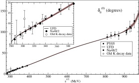
Figure 1: UFD for the $\pi\pi$ S0 wave. The dark band covers the uncertainties, versus the fitted data, namely, the “old” phase shift data from $K_{\ell 4}$ decays Rosselet:1976pu , the final NA48/2 results ULTIMONA48 and the data average performed in PY05 Pelaez:2004vs .

In Table 14, we show the experimental data considered, together with the fitted values and their corresponding residuals. In addition, in Fig. 1, we show the low energy conformal fit in detail, and in Table 9, we show the UFD parameters obtained from the fit.

II.3 Intermediate energy region: polynomial fit

This parametrization describes the S0 wave phase shift in the energy region between 850 and 1420 MeV. Below the $K\bar{K}$ threshold, it is fitted to the PY05 average of the different experimental solutions compatible with FDR Pelaez:2004vs , and to the re-analysis of the CERN-Munich experiments pipidata performed by Kaminski et al. Kaminski , which includes a huge estimation of the possible statistical uncertainties. Above the $K\bar{K}$ threshold, only were considered data sets with inelasticities compatible with $\pi\pi\rightarrow K\bar{K}$ scattering results in the region $4M_{K}^{2}\leq s\leq(1.25\,{\rm GeV})^{2}$ Wetzel:1976gw , namely, the solution $(-\,-\,-)$ of Hyams et al. Hyams75 , data of Grayer et al. Grayer and data of Kaminski et al.Kaminski . Unfortunately, data coming from Hyams75 only provided a statistical uncertainty estimation, so $5^{\circ}$ were added in GarciaMartin:2011cn as systematic error. In Fig. 2, we show the resulting polynomial fit and in Table 9, the UFD parameters obtained from the fit.

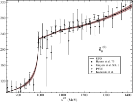
Figure 2: S0 UFD, where the dark band covers the uncertainties, versus the fitted data, namely, the data average performed in PY05 Pelaez:2004vs , the re-analysis of CERN-Munich experiments Kaminski , and data from Grayer ; Hyams75 .

In addition, as we did for the previous fit, in Table 15, we present the experimental data considered, together with the fitted values and their corresponding residuals.

II.4 S0 inelasticity fit

For the inelasticity, only data consistent with the dip solution were considered, namely the 1973 data of Hyams et al. pipidata , Protopopescu et al. pipidata and Kaminski et al.Kaminski . However, the data from Kaminski et al. were not included in the fit. As explained in GarciaMartin:2011cn , the reason behind this is that the main source of uncertainty was systematic, so the large number of points of Kaminski et al. together with the huge statistical errors would lead to a fit outcome with much smaller errors than the original systematic uncertainties. With only the other two sets, which are incompatible, a fit with a large $\chi^{2}/d.o.f.$ was obtained, and by rescaling its uncertainties in the inelasticity parameters, it was possible to mimic the dominant systematic uncertainties much better. Of course, the results were still in very good agreement with Kaminski et al. In Table 9 of the Appendix, we provide the values for the $\tilde{\epsilon}_{i}$ parameters, and in Fig. 3 we show the results of the unconstrained fit to the S0 wave inelasticity data up to 1420 MeV.

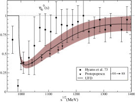
Figure 3: S0 inelasticity fit (UFD set) to the $\pi\pi\rightarrow\pi\pi$ scattering data of Hyams et al. (1973) and Protopopescu et al. As explained in the text, Kaminski et al. data were not fitted pipidata although the fit is compatible with them. The dark band covers our uncertainties.

III Normality test of the UFD fit

III.1 General remarks

In order to understand the discussion below, we have to introduce some well known concepts from the statistical theory of data analysis and specifically on normality tests. While the ideas are easy to grasp, these simple but extremely informative tests are too often overlooked as to deserve to be reviewed in some detail. We avoid on purpose the conventional statistical jargon which, after exchanging view with other researchers, usually backs off theoretical physicists from going in-depth through lengthy textbooks and use canned routines as a black box. The reader familiar with normality tests may skip this section.

As it is well known, the least squares method implicitly assumes that the residuals building the total $\chi^{2}$ are normally distributed. Of course, for a finite number of data, we can never be certain about this. We can however, estimate the probability by which we would err when we decide that this is not the case. In case we have no objection, we can plausibly assume that further measurements will decrease the uncertainties in the fitting parameters; otherwise we should expect incompatible determinations of fitting parameters.

In our case we want to decide whether or not the set of $N$ residuals $(R_{1},\dots R_{N})$ from the $\chi^{2}$-fit obey a standardized normal distribution. The question is whether or not the deviations of this empirical sample from the theoretical distribution can plausibly be attributed to the fact that number of data points $N$ is finite. This can be easily done by generating random numbers drawn from a normal distribution $(\xi_{1},\dots,\xi_{N})$, $\xi_{i}\in N(0,1)$, and comparing some quantity of interest $T(\xi_{1},\dots,\xi_{N})$ with the actually observed empirical result $T_{\rm obs}=T(x_{1},\dots,x_{N})$. Of course, we can repeat the process as many times $a=1,\dots,M$ as we want and we will obtain a spread of results $T_{\rm th,a}=T(\xi_{1,a},\dots,\xi_{N,a})$ yielding a distribution of values for the variable $T$ assuming the variables $(\xi_{1,a},\dots,\xi_{N,a})$ are uncorrelated normal variables.

A very important issue is to agree on what quantity should be used for this comparison. Let us consider, for instance, the moments centered at the origin defined as:

$$\mu_{r}(x_{1},\dots,x_{N})=\frac{1}{N}\sum_{i=1}^{N}x_{i}^{r},$$ (17)

Of course, for normally distributed variables $\mu_{r}(\xi_{1},\dots,\xi_{N})$ becomes a random variable itself which follows a certain distribution,

$$P_{N}(\mu_{r})=\langle\delta(\mu_{r}-\mu_{r}(\xi_{1},\dots,\xi_{N}))\rangle,$$ (18)

where the expectation value is defined as:

$$\langle O\rangle_{N} = \int_{-\infty}^{\infty}d\xi_{1}\frac{e^{-\xi_{1}^{2}/2}}{\sqrt{2\pi}}\dots\int_{-\infty}^{\infty}d\xi_{N}\frac{e^{-\xi_{N}^{2}/2}}{\sqrt{2\pi}}O(\xi_{1},\dots,\xi_{N}).$$

This function cannot be computed analytically, except for $r=1,2$ or when $N\to\infty$ (featuring the central limit theorem evans2004probability ),

$$P_{N}(\mu_{r})\to\frac{e^{-\frac{1}{2}\left[\frac{\mu_{r}-\langle\mu_{r}\rangle}{\Delta\mu_{r}}\right]^{2}}}{\sqrt{2\pi}\Delta\mu_{r}},$$ (20)

where the mean $\langle\mu_{r}\rangle$ and the standard deviation $(\Delta\mu_{r})^{2}=\langle\mu_{r}^{2}\rangle-\langle\mu_{r}\rangle^{2}$ can be expressed in terms of Euler’s gamma functions evans2004probability . The lowest values $r\leq 8$ are listed for a quick reference in Table 1. Thus, we have that if $x_{i}\in N[0,1]$ then within $1\sigma$ ($68\%$) confidence level and for large $N$,

$$\frac{1}{N}\sum_{i=1}^{N}z_{i}^{r}=\langle\mu_{r}\rangle\pm\Delta\mu_{r}.$$ (21)

When $N$ is not as large (say $\lesssim 30$) one can proceed by Monte Carlo by sampling $N$ gaussian numbers and computing the distribution of moments.

Table 1: The normalized moments $\mu_{r}$ of the standardized gaussian distribution with their mean standard deviation $\Delta\mu_{r}$ for a sample of size $N$. For normal distributed data $x_{i}\in N(0,1)$ we expect that to $1\sigma$ confidence level $\sum_{i=1}^{N}x_{i}^{r}/N=\mu_{r}\pm\Delta\mu_{r}$.

$r$	0	1	2	3	4	5	6	7	8
$\mu_{r}$	1	0	1	0	3	0	15	0	105
$\Delta\mu_{r}$	0	$\frac{1}{\sqrt{N}}$	$\frac{\sqrt{2}}{\sqrt{N}}$	$\frac{\sqrt{15}}{\sqrt{N}}$	$\frac{4\sqrt{6}}{\sqrt{N}}$	$\frac{3\sqrt{105}}{\sqrt{N}}$	$\frac{3\sqrt{1130}}{\sqrt{N}}$	$\frac{3\sqrt{15015}}{\sqrt{N}}$	$\frac{240\sqrt{35}}{\sqrt{N}}$

In the moments method we weight the tails more strongly as the power $r$ increases. Therefore, rejecting or accepting normality on the basis of each individual moment $\mu_{r}$ tests different features of the distribution. This discussion shows that normality is to some extent in the eyes of the beholder, and generally it is better to use different tests.

As we have already mentioned, the modeling of data requires an assumption both for the signal (the fitting curve) and the noise (the statistical fluctuation). In this regard, there is an interesting situation where the moments do not stem from a standardized normal distribution, but after suitably shifting and re-scaling they do. In such a case we can still propagate errors according to the shifted and re-scaled distribution.

III.2 Normality tests

The normality test consists of an a priori criterium where one decides if the set of data $(x_{1}\dots,x_{N})$ could possibly be normal. To make this decision, one evaluates what is the probability $p$ of making an erroneous decision of denying the normality of the residuals. The $p$-value is obtained by locating an observable $T$, known as test statistic, from the actual empirical data $(x_{1},\dots,x_{N})$ in the theoretical distribution that this expected in case the data do follow the normal distribution. A small $p$-value indicates clear deviations from the normal distribution, whereas a large $p$-value indicates that no statistically significant discrepancies were found. When comparing $T_{\rm obs}$ to the distribution of $T$ a significance level $\alpha$ is arbitrarily chosen, this determines a critical value $T_{c}$. Common choices for $\alpha$ are $0.01$ and $0.05$. We then compare the observed $T$ with the critical theoretical value $T_{c}$. The definition of $T$ in each test determines which inequality must be fulfilled either from the left or the right. Therefore $T\geq T_{c}$  the assumption that the empirical data $x_{1},\dots,x_{n}$ were drawn from the probability distribution $\rho(x)$ can be rejected with a confidence level of $100(1-\alpha)\%$. If $T<T_{c}$ there are no statistically significant reasons to reject the assumption. This is usually expressed in short saying that the finite sample $(x_{1},\dots,x_{N})$ follows the normal distribution $N(0,1)$ with $100(1-\alpha)\%$ confidence level.

There are many tests available on the market, and we will take here the most popular, which are the Pearson, Kolmogorov-Smirnov (KS) and Tail-Sensitive (TS) tests. We will also use the moments method already described above.

III.2.1 Pearson test

The Pearson test is one of the first tools used to test the goodness of fit by comparing the histograms of the empirical data (the residuals of a fit in this case) and of the normal distribution. For this purpose a binning must be specified and the data is binned accordingly and the test statistic is defined as

$$T_{\rm Pearson}=\sum_{i=1}^{Nb}\frac{\left(n_{i}^{\rm res}-n_{i}^{\rm normal}\right)^{2}}{n_{i}^{\rm normal}},$$ (22)

where $N_{b}$ is the number of bins, $n_{i}^{\rm fit}$ is the number of residuals on each bin and $n_{i}^{\rm normal}$ the expected number of data from a normal distribution on the same bin. In this case a large value of $T_{\rm Pearson}$ indicates discrepancies between the empirical and normal distribution and therefore the null hypothesis is rejected if $T_{\rm obs}>T_{c}$.

One particular disadvantage of the Pearson test is the dependence of $T_{\rm obs}$ on the number and size of the bins, which are set arbitrarily. Different choices can be made about the binning, usual methods employ equiprobable bins so that $n_{i}^{\rm normal}$ is constant; while others use a binning with a constant bin size (see e.g. Ref. eadie2006statistical for more details on binning strategies).

III.2.2 Kolmogorov-Smirnov Test

The Kolmogorov-Smirnov test (KS) quantifies the discrepancies between two distributions by comparing their cumulative distribution functions (CDF). In the case of a set of $N$ empirical data $X_{i}$, the CDF corresponds to the fraction of data that is smaller than a certain value $x$ i.e.

$$S_{N}(x)=\frac{1}{N}\sum_{i=1}^{N}\theta(x-x_{i}).$$ (23)

The CDF of the normal distributions is given by

$$\Phi(x)=\frac{1}{\sqrt{2\pi}}\int_{-\infty}^{x}dte^{-t^{2}/2}.$$ (24)

The test statistic of this test is defined as the maximum value of the absolute difference between both cumulative distribution functions, that is

$$T_{\rm KS}=\max_{-\infty<x<\infty}|S_{N}(x)-\Phi(x)|.$$ (25)

Another advantage of the KS normality test is that a good approximation for the $p$-value exist and is given by

$$P_{\rm KS}(T_{\rm obs})=2\sum_{j=1}^{\infty}(-1)^{j-1}e^{-2\left[\left(\sqrt{N}+0.12+0.11/\sqrt{N}\right)jT_{\rm obs}\right]^{2}}.$$ (26)

This approximation is sufficiently good for $N>4$ and approaches the actual value asymptotically as $N$ becomes larger.

For a normal distribution $x_{i}\in N[0,1]$ one has that for large $N$ and within $1\sigma$ confidence level,

$$S_{N}(x)=\phi(x)\pm\frac{1}{\sqrt{N}}\sqrt{\phi(x)(1-\phi(x))}\,.$$ (27)

As in the Pearson test, a large value for $S_{N}(x)$ indicates larger discrepancies with the normal distribution and therefore the null hypothesis will be rejected if $T_{\rm KS}$ is larger than a certain critical values $T_{c,\rm KS}$. The critical values depend on the sample size $N$ and level of significance $\alpha$ with tables for common values of $\alpha$ and $N\leq 40$ readily available in the literature. These same tables usually include a fairly good approximation for $N>40$, the more common case in testing normality of residuals from a least squares fit, which we reproduce here as a quick reference in table 2.

Table 2: Large $N$ parametrization of the critical values for the Kolmogorov-Smirnov normality test $T_{\rm c}=a/\sqrt{N}$ at different levels of significance. This approximation is appropriate for $N<40$

	$\alpha$				a
	0.01				1.63
	0.02				1.52
	0.05				1.36
	0.10				1.22
	0.20				1.07

III.2.3 QQ plot and tail sensitive test

The idea of the Tail Sensitive (TS) test comes from the normal quantile-quantile (QQ) plot, where one compares one to one the empirical points $x_{1}<\dots<x_{N}$ with the theoretical points

$$\frac{n}{N+1}=\int_{-\infty}^{x_{n}^{\rm th}}dx\frac{e^{-x^{2}/2}}{\sqrt{2\pi}}\,,$$ (28)

If the empirical points follow a Normal distribution the QQ-plot corresponds to the straight line rotated $45^{0}$, $x_{n}=x_{n}^{\rm th}$. A good feature of this representation is that the tails are stretched which makes it very suitable to analyze data selection where possible outliers are discarded (see Sect. VI). The TS test defines the test statistic as

$$T_{\rm TS} = 2\min_{i}\left\{\min\left[B_{i,N+1-i}(z_{i}),1-B_{i,N+1-i}(z_{i})\right]\right\},$$

where the cumulative distribution function corresponds to the regularized incomplete Beta-function and is defined as

$$B_{i,N+1-i}(z)=\sum_{j=i}^{N}\left(\begin{array}[]{c}N\\ j\end{array}\right)z^{j}(1-z)^{N-j},$$ (30)

and the mapping between $N[0,1]\to U[0,1]$

$$z_{i}=\frac{1}{\sqrt{2\pi}}\int_{-\infty}^{x_{i}}dxe^{-x^{2}/2},$$ (31)

has been introduced. In Ref. Perez:2014kpa the critical $T_{c}$ was tabulated for $N\leq 50$ and parametrized for $N>50$ as

$$T_{c}=\frac{a}{\sqrt{N}}+b,$$ (32)

for the usual significance levels of $\alpha=0.2,0.1,0.05,0.02,0.01$.

IV Testing the UFD fits

After the fitting process and the normality tests have been introduced, let us now face the original UFD S0 wave fit from GarciaMartin:2011cn against them. As mentioned above, this is equivalent to check whether the statistical assumptions implicit in the standard least squares $\chi^{2}$ fitting procedure are satisfied. Therefore, we will start computing the resulting residuals of the fit, defined by Eq. (3) where ${\cal O}_{i}$ denotes the fitted observable, i.e. phase shift or inelasticity data, and that should follow a normal distribution within a given confidence level

As we have pointed out in the previous section, a quantitative way to study the normal behavior of the residual distribution is to analyze its central moments, which in the discrete case are defined through,

$$\mu_{n}=\frac{1}{N}\sum_{i=1}^{N}{(R_{i}-R_{\rm mean})^{n}}.$$ (33)

In this way, we can compare whether they are compatible within uncertainties with the expected moments of $N$ random data points normally distributed, where again, $N$ is the total number of residual and the moment error is given by the square of its variance. We can also check whether this situation improves when we consider a normalized residual distribution,

$$\hat{R}_{i}=\frac{R_{i}-R_{\rm mean}}{\sqrt{V(R)}},$$ (34)

where, $R_{\rm mean}=\Sigma_{i}^{N}{R_{i}}/N$ is the expected value of the residual and $V(R)=\Sigma_{i}^{N}(R_{i}-R_{\rm mean})^{2}/(N-1)$ is its variance. In this case, the central moments of the distribution of the normalized residuals are given by:

$$\hat{\mu}_{n}=\frac{1}{N}\sum_{i=1}^{N}{(\hat{R}_{i}-\hat{R}_{\rm mean})^{n}}.$$ (35)

For completeness, in Table 16, we show the experimental data considered, together with the fitted values and their corresponding residuals. Since the analysis of elastic $\pi\pi$ scattering in the $0^{++}$ channel was done separately in the low energy region and intermediate region and also independently from the inelastic scattering data, we have to pose the question on normality in a separate fashion.

IV.1 Low energy region

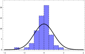
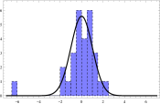
Figure 4: Left: histograms of the resulting residuals after fitting the S0 wave data. Right: rescaled residual histogram. Upper panels: Data described with conformal parametrization. Middle panels: Data described by the polynomial parametrization. Lower panels: Inelastic data. The black curve corresponds to an analytical normal distribution.

In the upper left panel of Fig. 4, we show for the conformal low energy fit the distribution of the resulting residuals given in Eq. (3) compared with the analytical Gaussian distribution. We can conclude directly from this plot that it is not justified to assume that they follow a normal distribution. There is an excess of events in the origin.

In addition, in Table 3 we show in both cases their first moments. By definition, the first two moments are $\mu_{0}=1$, $\mu_{1}=0$. However, for the variance $\mu_{2}$, we obtain a tiny deviation, which points out that the distribution of residuals cannot be considered Gaussian. Since the sample of low energy points ($N=30$) is rather small, for higher values of $n$, the Gaussian moment uncertainties increase considerably, ensuring that the residual moments are going to be satisfied within uncertainties.

	$\mu_{0}$	$\mu_{1}$	$\mu_{2}$	$\mu_{3}$	$\mu_{4}$	$\mu_{5}$	$\mu_{6}$
$R_{\rm old}$	1	0	0.6	0.0	1.5	0.1	4.2
$N(0,1)_{\rm old}$	$1\pm 0$	$0\pm 0$	$1.0\pm 0.3$	$0.0\pm 0.5$	$2.8\pm 2.1$	$0\pm 6$	$14\pm 30$
$R_{\rm new}$	1	0	0.9	-0.1	2.1	-0.2	7
$N(0,1)_{\rm new}$	$1\pm 0$	$0\pm 0$	$1.0\pm 0.3$	$0.0\pm 0.5$	$2.8\pm 1.9$	$-0.1\pm 5$	$14\pm 19$
	$\hat{\mu}_{0}$	$\hat{\mu}_{1}$	$\hat{\mu}_{2}$	$\hat{\mu}_{3}$	$\hat{\mu}_{4}$	$\hat{\mu}_{5}$	$\hat{\mu}_{6}$
$\hat{R}_{\rm old}$	1	0	1	0	3.5	0.4	16
$\hat{N}(0,1)_{\rm old}$	$1\pm 0$	$0\pm 0$	$1\pm 0$	$0.0\pm 0.4$	$2.5\pm 0.6$	$0\pm 3$	$10\pm 7$
$\hat{R}_{\rm new}$	1	0	1	-0.1	2.6	-0.3	9
$\hat{N}(0,1)_{\rm new}$	$1\pm 0$	$0\pm 0$	$1\pm 0$	$0.0\pm 0.4$	$2.6\pm 0.7$	$0\pm 3$	$11\pm 7$

Table 3: Central moments of the distribution of residuals obtained for the low energy conformal fit versus the moments of N random points normally distributed. The subscripts “old” and “new” denote respectively the original UFD and the UFD for the new selection of data performed in Section V. $\mu_{0}$ and $\mu_{1}$ are by definition 1 and 0 respectively. However for $\mu_{2}$, very small deviations appear for the original UFD. For higher values of $n$, they are always compatible due to huge uncertainties coming from a small sample of points (N=30). In contrast, for the new selection of data all moments are compatible with the expected values of a gaussian distribution. The last four rows contain the central moments of the normalized residual distribution obtained in the conformal fit versus the moments of N normalized random points normally distributed.

In the upper right panel of Fig. 4, we show the normalized residual histogram, where we can see, that, despite an important improvement, it does not correspond to a normal distribution. This can be again checked by comparing the last two rows in Table 3, where we show the central moments of the normalized residual distribution and those of a rescaled Gaussian distribution of N random points. The first deviations occur for $\hat{\mu}_{4}$. Therefore, we can conclude that although only slightly, the low energy S0 wave phase shift UFD fit from GarciaMartin:2011cn violates the residual normality test. However, this small violation anticipates tiny corrections to the results obtained in GarciaMartin:2011cn .

IV.2 Intermediate energy

As we did for the low energy case, we will start analyzing the normal behavior of the intermediate energy S0 wave phase shift fit by studying the behavior of its residuals. Their normalized and rescaled distributions are plotted in the middle panel of Fig. 4, and point out again a excess of residual at the origin, and consequently a non-gaussian behavior. As we proceeded for the previous fit, in order to quantify this deviation, we compute again the moments for the normal and rescales residual distributions. The results are given in Table 4.

	$\mu_{0}$	$\mu_{1}$	$\mu_{2}$	$\mu_{3}$	$\mu_{4}$	$\mu_{5}$	$\mu_{6}$
$R_{\rm old}$	1	0	0.5	-0.3	1.3	-2	7
$N(0,1)_{\rm old}$	$1\pm 0$	$0\pm 0$	$1.0\pm 0.2$	$0.0\pm 0.3$	$2.9\pm 1.2$	$0\pm 3$	$14\pm 12$
$R_{\rm new}$	1	0	0.8	0.0	1.3	-0.2	4
$N(0,1_{\rm new})$	$1\pm 0$	$0\pm 0$	$1.0\pm 0.2$	$0.0\pm 0.3$	$2.8\pm 1.2$	$-0.2\pm 3$	$14\pm 11$
	$\hat{\mu}_{0}$	$\hat{\mu}_{1}$	$\hat{\mu}_{2}$	$\hat{\mu}_{3}$	$\hat{\mu}_{4}$	$\hat{\mu}_{5}$	$\hat{\mu}_{6}$
$\hat{R}_{\rm old}$	1	0	1	-0.8	5.2	-12	53
$\hat{N}(0,1_{\rm old})$	$1\pm 0$	$0\pm 0$	$1\pm 0$	$0.0\pm 0.3$	$2.8\pm 0.5$	$0\pm 3$	$13\pm 8$
$\hat{R}_{\rm new}$	1	0	1	0.1	2.4	0.6	8
$\hat{N}(0,1)_{\rm new}$	$1\pm 0$	$0\pm 0$	$1\pm 0$	$0.0\pm 0.3$	$2.7\pm 0.6$	$0\pm 3$	$12\pm 8$

Table 4: Central non- and normalized moments for the residuals of the intermediate energy polynomial parametrization for the original and new UFD of Section V.

Since for the intermediate energy region the sample of points is bigger ($N=61$), the expected errors are smaller and the residual constraint becomes this time much more stringent. For the non-rescaled case we can see small deviation for $\mu_{2}$ and $\mu_{4}$, proving again a non Gaussian behavior. For the rescaled case bigger deviations occur for $n>3$.

IV.3 Inelastic data

In the case of the S0 wave inelasticity, the non- and normalized distribution of the residuals are plotted in the lower panel of Fig. 4. In this case, the main problem does not come from an excess of events at the origin, but for some values which are far away from it, in contradiction with a gaussian behavior. The central moments of both distributions are given in Tab. 5 and they show that, despite we are working with a small sample ($N=28$) and the expected errors are big, there are severe deviations, some of them of more than an order of magnitude.

	$\mu_{0}$	$\mu_{1}$	$\mu_{2}$	$\mu_{3}$	$\mu_{4}$	$\mu_{5}$	$\mu_{6}$
$R_{\rm old}$	1	0	2.2	-7.9	54	-318	1981
$N(0,1)_{\rm old}$	$1\pm 0$	$0\pm 0$	$1.0\pm 0.2$	$0.0\pm 0.4$	$3.0\pm 1.3$	$0\pm 3$	$14\pm 12$
$R_{\rm new}$	1	0	0.8	0.0	1.9	0.0	6
$N(0,1_{\rm new})$	$1\pm 0$	$0\pm 0$	$1.0\pm 0.2$	$0.0\pm 0.3$	$2.8\pm 1.2$	$0\pm 3$	$14\pm 11$
	$\hat{\mu}_{0}$	$\hat{\mu}_{1}$	$\hat{\mu}_{2}$	$\hat{\mu}_{3}$	$\hat{\mu}_{4}$	$\hat{\mu}_{5}$	$\hat{\mu}_{6}$
$\hat{R}_{\rm old}$	1	0	1	-0.8	5.2	-12	53
$\hat{N}(0,1)_{\rm old}$	$1\pm 0$	$0\pm 0$	$1\pm 0$	$0.0\pm 0.3$	$2.8\pm 0.5$	$0\pm 3$	$13\pm 7$
$\hat{R}_{\rm new}$	1	0	1	0.1	2.4	0.6	8
$\hat{N}(0,1)_{\rm new}$	$1\pm 0$	$0\pm 0$	$1\pm 0$	$0.0\pm 0.3$	$2.8\pm 0.5$	$0\pm 3$	$13\pm 7$

Table 5: Central moments of the residual distribution obtained for the S0 wave inelasticity for the original (old) and new selection of data (new) (Section V). In the case of the original UFD, there are very severe deviation with respect to a normal distribution. On the contrary, for the new selection of data, the agreement is remarkable.

IV.4 Quantitative checks

Table 6: Results of the Pearson normality test of the residuals obtained by fitting the different data sets with the conformal, polynomial and inelastic parametrizations. The results of the test of the scaled residuals for every case is shown below the corresponding line. The critical value $T_{c}$ corresponds to a significance level of $\alpha=0.05$.

Database	Fit	$N$	$T_{c}$	$T_{\rm obs}$	$p$-value
Conformal	UFD	$30$	$14.07$	$14.80$	$0.039$
				$10.43$	$0.021$
Conformal new	UFD	$25$	$14.07$	$5.40$	$0.611$
				$5.40$	$0.611$
Polynomial	UFD	$61$	$18.31$	$21.05$	$0.021$
				$6.98$	$0.727$
Polynomial new	UFD	$52$	$16.92$	$4.15$	$0.901$
				$3.00$	$0.964$
Inelastic	UFD	$28$	$14.07$	$5.14$	$0.642$
				$6.71$	$0.573$
Inelastic new	UFD	$27$	$14.07$	$2.93$	$0.892$
				$2.93$	$0.892$

Table 7: Same as table 6 for the Kolmogorov-Smirnov test

Database	Fit	$N$	$T_{c}$	$T_{\rm obs}$	$p$-value
Conformal	UFD	$30$	$0.242$	$0.253$	$0.036$
	UFD			$0.216$	$0.105$
Conformal new	UFD	$25$	$0.264$	$0.158$	$0.513$
	UFD			$0.157$	$0.520$
Polynomial	UFD	$61$	$0.174$	$0.170$	$0.053$
	UFD			$0.097$	$0.582$
Polynomial new	UFD	$52$	$0.189$	$0.082$	$0.846$
	UFD			$0.058$	$0.991$
Inelastic	UFD	$28$	$0.250$	$0.118$	$0.785$
	UFD			$0.186$	$0.254$
Inelastic new	UFD	$27$	$0.254$	$0.140$	$0.611$
	UFD			$0.129$	$0.715$

Table 8: Same as table 6 for the tail sensitive test

Database	Fit	$N$	$T_{c}$	$T_{\rm obs}$	$p$-value
Conformal	UFD	$30$	$0.0039$	$0.0049$	$0.061$
	UFD			$0.0155$	$0.164$
Conformal new	UFD	$25$	$0.0042$	$0.1662$	$0.794$
	UFD			$0.1686$	$0.799$
Polynomial	UFD	$61$	$0.0027$	$0.0010$	$0.020$
	UFD			$0.0081$	$0.132$
Polynomial new	UFD	$52$	$0.0029$	$0.0912$	$0.681$
	UFD			$0.3101$	$0.988$
Inelastic	UFD	$28$	$0.0040$	$1.2\times 10^{-8}$	$0.0002$
	UFD			$0.001$	$0.016$
Inelastic new	UFD	$27$	$0.0040$	$0.1505$	$0.769$
	UFD			$0.1913$	$0.851$

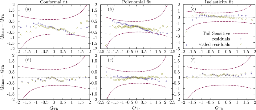
Figure 5: (Color online) Rotated Quantile-Quantile plots for residuals of different fits. Left panels: low energy conformal fits. Middle panels: intermediate energy polynomial fits. Right panels: high energy inelasticity fits. Upper panels: fit to the original database. Lower panels: fit to the newly selected data. The resulting residuals are marked as blue vertical crosses and the scaled ones as yellow diagonal crosses. The $95\%$ confidence bands from the TS normality test are also shown (dashed red line).

On a more quantitative level, we complement the previous results with Tables 6,7 8 for the Pearson, KS and TS tests respectively. It is interesting to note that for the Pearson and KS tests the p-value is very high for the Inelastic fit, whereas the TS gives a too low value. This is mainly due to the outlier with $R_{i}=-6.24$ sitting at the tail of the distribution. We also note that for these small data points values ($N$), the power of the test (probability of not giving a false positive) is low. Finally, QQ-plots are shown in Fig. 5. All this reinforces the lack of normality of residuals.

V New selection of data

The results presented in Section IV highlight that the UFD fits to the $\pi\pi$ scattering amplitude in the $0^{++}$ channel from GarciaMartin:2011cn do not satisfy a posteriori the statistical assumptions implicit in the $\chi^{2}$ minimization. This inconsistency in the $\chi^{2}$ fit can be due to either the presence of mutually incompatible data or a biased choice of the fitting curve. We will explore the consequences that a new selection of data implies regarding normality of residuals.

V.1 New selection of low energy data

As we have seen before, there are three different sets of experiments included in the low energy region. The NA48/2 set ULTIMONA48 corresponds to the newest data on $K_{\ell 4}$ decays and incorporates a rigorous statistical and systematic error analysis, so there is no reason to modify or alter this set of data. As we have commented before, the PY05 average selection corresponds to an average of the different experimental solutions that passed a consistency test with FDR and other sum rules. The large uncertainties assigned covered the difference between the different data sets, and at some point, they can be considered arbitrary. Since, as we can see in upper Fig. 4, there is an excess of residuals at the origin, it is reasonable to assume that they may be overestimated. The last set of data considered in the low energy fit corresponds to old data on $K_{\ell 4}$ decays from Rosselet:1976pu , whose precision cannot be consider as the same level than the recent NA48/2 analysis. Therefore, it makes sense to get rid of those old data points on $K_{\ell 4}$ decays which lie within uncertainties in the same energy bin than a NA48/2 value. Thus, in order to improve the Gaussian check of the fit, we divide by two the uncertainty of the PY05 data average and get rid of the old K decay corresponding to the following values of $\sqrt{s}$, {289, 317, 324, 340, 367}. The comparison of the tiny differences between the old and the new fit is plotted in Fig. 6. Its corresponding parameters are given in Table 9.

Figure 6: Old versus new UFD at low energies, the dark band covers the uncertainties of the old parametrization.

Finally, in the upper panel of Fig. 7, we plot the residual distribution for the new fit. Despite there are still some deviations, there is a clear improvement, which can be again checked by computing the central moments of the distribution. They are given in Table 3, showing a complete agreement between them and the expected values of N random points normally distributed.

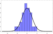
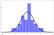
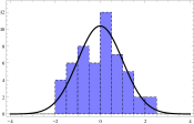
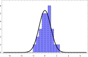
Figure 7: Same as Fig. 4 for the new data selection.

In this was, by imposing the Gaussian check in the data selection, we are able to constraint part of the arbitrariness assumed in the data selection, namely, the systematic uncertainty taken for the PY05 average and the old K decay data points considered.

V.2 New selection of intermediate energy data

On the one hand, as we can can see in middle Fig. 4, there is again a excess of residuals in the central region, i.e. for $R\sim 0$, which could be considered as a signal of overestimated uncertainties. On the other hand, the uncertainties of the PY05 average data, the systematic error added to Hyams and the errors given by Kaminski et al. can be considered at some point arbitrary. Therefore, in order to improve the normal behavior of the residual distribution, we reduce by a factor 1/2 the uncertainties of the PY05 average, we sum $3^{\circ}$ instead of $5^{\circ}$ as systematic uncertainty to the data from Hyams, and rescale by a factor of 3/4 the uncertainties of Kaminski data. In addition, since there are several Kaminski data points which are compatible with those of Grayer, Hyams or PY05 but with higher uncertainties, we get rid of the Kaminski data point at the following energies {930,970,1010,1050,1210,1390}. The normalized and rescaled distribution of the residuals for the new data selection are plotted in middle Fig. 7, whereas the central moments are given in Table 4. Despite there are still some deviations, the improvement is clear. The value of the parameters corresponding to the new polynomial fit are given in Table 9, and the comparison between the new and old polynomial curve is plotted in Fig. 8.

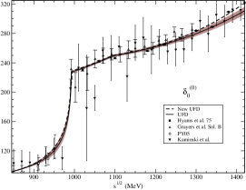
Figure 8: Old versus new UFD for the polynomial parametrization, the dark band covers the uncertainties of the old parametrization.

V.3 New selection of inelasticity data

In this case, as we can see in the histograms depicted in the lower panel of Fig. 4, rather than by overestimated errors, the problem comes from incompatible data points, and in particular for the Hyams data point at $\sqrt{s}=994$ MeV. If we simply get rid of this point, the new fit improves striking the normal behavior as we can see in the lower panel of Fig. 7. The central moments of the new fit are given in Table 5, and show a perfect agreement. The new inelasticity parameters are given in Table 9, and the difference between the old and new parametrizations are plotted in Fig. 9.

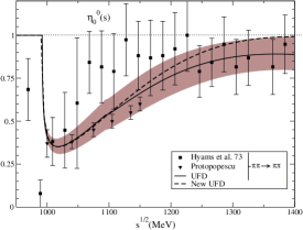
Figure 9: Old versus new UFD for the inelasticity, the dark band covers the uncertainties of the old parametrization.

S0 wave	UFD	New UFD
$B_{0}$	$7.26\pm 0.23$	$7.38\pm 0.23$
$B_{1}$	$-25.3\pm 0.5$	$-24.5\pm 0.5$
$B_{2}$	$-33.1\pm 1.2$	$-35.4\pm 1.2$
$B_{3}$	$-26.6\pm 2.3$	$-34.7\pm 2.7$
$z_{0}$	$M_{\pi}$	$M_{\pi}$
$\chi^{2}/\nu$	$0.645$	$1.111$
$1-\sqrt{2/\nu}$	$0.723$	$0.691$
$1+\sqrt{2/\nu}$	$1.277$	$1.309$
$d_{0}$	$(227.1\pm 1.3)^{\circ}$	$(228.8\pm 1.3)^{\circ}$
$c$	$(-660\pm 290)^{\circ}$	$(-466\pm 294)^{\circ}$
$B$	$(94.0\pm 2.3)^{\circ}$	$(85.1\pm 2.3)^{\circ}$
$C$	$(40.4\pm 2.9)^{\circ}$	$(60.7\pm 2.9)^{\circ}$
$D$	$(-86.9\pm 4.0)^{\circ}$	$(-92.3\pm 4.0)^{\circ}$
$\chi^{2}/\nu$	$0.552$	$0.761$
$1-\sqrt{2/\nu}$	$0.811$	$0.794$
$1+\sqrt{2/\nu}$	$1.189$	$1.206$
$\tilde{\epsilon}_{1}$	$4.7\pm 0.2$	$4.6\pm 0.1$
$\tilde{\epsilon}_{2}$	$-15.0\pm 0.8$	$-14.6\pm 0.4$
$\tilde{\epsilon}_{3}$	$4.7\pm 2.6$	$3.9\pm 4.4$
$\tilde{\epsilon}_{4}$	$0.38\pm 0.34$	$0.37\pm 0.20$
$\chi^{2}/\nu$	$2.668$	$1.039$
$1-\sqrt{2/\nu}$	$0.711$	$0.705$
$1+\sqrt{2/\nu}$	$1.289$	$1.294$

Table 9: S0 wave parameters for the old and new UFD sets, indicating also the number of fitted data $N$, the corresponding $\chi^{2}/\nu$ and expected value boundaries $1\pm\sqrt{2/\nu}$. The first set corresponds to the low energy parametrization, $\sqrt{s}\leq 0.85\,\mathrm{GeV}$, the second set to the intermediate energy conformal fit and the last one to the inelastic parametrization up to $\sqrt{s}=1.42\,\mathrm{GeV}$.

V.4 Resonance pole parameters

As it has been pointed out in the introduction, one of the main achievements of the dispersive $\pi\pi$ analyses based on Roy and Roy-like equations Ananthanarayan:2000ht ; Colangelo:2001df ; GarciaMartin:2011cn has been the precise and unbiased determination of the lowest scalar resonance states Caprini:2005zr ; GarciaMartin:2011jx , namely, the $f_{0}(500)$ and $f_{0}(980)$. In particular, in GarciaMartin:2011jx , the CFD parametrizations of GarciaMartin:2011cn were used as input for the analytic extrapolation to the complex plane of the dispersive once- and twice-subtracted Roy equation, and thus, allowing to look for the lowest-lying poles on the second Riemann sheet. Therefore, it is relevant to check the effect of the new selection of data on the scalar pole determinations. In Table 10, we show the pole positions of the $f_{0}(500)$ and $f_{0}(980)$ resonances for the old and new UFD, obtained from the twice-subtracted Roy equations. For completeness, we also show the results for the $\rho(770)$ resonance. Note that the values of the $\rho$ pole depend on the new S0 wave data selection through the dispersive integral. The small differences between both determinations point out the small effects of the new data selection and reinforce the results obtained in GarciaMartin:2011jx .

	old UFD(MeV)	new UFD (MeV)
$\sqrt{s_{f_{0}(500)}}$	$(482\pm 16)-i(268\pm 16)$	$(483\pm 17)-i(266\pm 16)$
$\sqrt{f_{0}(980)}$	$(1001\pm 3)-i(8\pm 9)$	$(1001\pm 5)-i(12\pm 10)$
$\sqrt{\rho(770)}$	$(764.4\pm 2.0)-i(73.3\pm 1.2)$	$(764.2\pm 1.9)-i(73.2\pm 1.2)$

Table 10: $f_{0}(500)$, $f_{0}(980)$ and $\rho(770)$ resonance pole positions of the old and new UFD obtained from the analytic continuation to the complex plane of the twice subtracted Roy equation GarciaMartin:2011cn . The tiny differences between both determinations strengthen the error analysis carried out in GarciaMartin:2011cn .

VI Elements of a self-consistent fit

As we have mentioned and demonstrated in the previous section, the selection of data is an essential ingredient for a self-consistent fit, namely a fit where residuals follow a normal distribution. However, this selection has been done by hand, and a more general procedure would be most useful. Guided by previous experience in NN scattering Perez:2014yla ; Perez:2014kpa we try to explore a similar selection method.

Of course, one important aspect is that, unless specifically proven incorrect, all available data as they are published by the experimentalists should be taken into account to make the data selection. However let us remember that, in the particular case of $\pi\pi$ scattering, phase shift and inelasticity data are not obtained from direct measurements, but indirect, requiring the use of models, and thus, involve systematic uncertainties. Note by instance, that the PY05 average Pelaez:2004vs used in both, the conformal and intermediate-energy parametrizations of GarciaMartin:2011cn was obtained confronting these experimental analyses against Forward dispersion relations.

Nevertheless, if in general we assume from the start that all experiments are correct; our goal is to reach a consensus among published experimental data which are or could be mutually compatible. This is an important assumption, but it is the most objective one we can make without any detailed knowledge on how the experimental analysis was carried out; if we did know, we would decide based on our own judgement. We hope, however, that given a sufficiently large number of data, statistical analysis will help us to make a judicious choice and to reach a consensus among individual data measurements. In this way, we envisage the possibility that simple experimental values in a given experiment can individually be discarded without questioning the whole experiment. A practical way to implement this method is to follow the $3\sigma$ self-consistent procedure proposed in Perez:2013jpa , which is given by the following three-steps algorithm: i) Make a first and global fit, ii) Discard from all data those fulfilling $R_{i}^{2}>9$ iii) Re-fit the remaining data and go to step ii) until convergence. This selection method will generate a boundary between accepted and rejected data and there will be a flow of data across the boundary during the iterative process.

The good feature of this method is that in the case of two mutually incompatible data it helps to decide which one is better suited even when initially and individually one would reject both. Of course, this decision is controlled by the fitting theory and unforeseen restrictions on the theory may induce an undesirable bias in our choice. It is thus important that the fitting curve is flexible enough to prevent this situation . Note that after this process has been carried out, we have still to check whether the residuals pass the normality test.

In order to check the disagreement between the $\pi\pi$ data sets considered in the previous sections, we apply the self-consistent approach to the S0 wave phase shift, performing a global fit to the data sets described in Sect.IV.1 and IV.2. The advantage of a global fit, instead of considering separately the low and energy region, is that we can treat on an equal footing both energy regions, and thus, without introducing a priory any bias into our analysis. Note, however, that the hierarchy imposed in the original work of GarciaMartin:2011cn , allows to take advantage of the high precision accomplished in the latest NA48/2 ULTIMONA48 .

In all, we find that if we fit the data in the S0 up to $\sqrt{s}=1.42\,{\rm GeV}$ convergence is achieved already with two iterations, with a total of only three points being discarded, namely, the “old” K decay data point Rosselet:1976pu at $\sqrt{s}=381.4$ MeV, (Table 14) and the Kaminski et al. Kaminski data points at $\sqrt{s}=\{970,1050\}$ MeV, (Table 15). In Table 13, we provide the resulting parameters in the first and second iterations. Note that the differences between the new UFD parameters and the original ones Table 9 are due to the global fit we are performing in the self-consistent method.

As compared to the more detailed discussion in the previous section, it is fair say that the $3\sigma$ self-consistent approach is much simpler and effective, and does not require from the theoretician’s side a detailed discussion of the published data but rests on the assumption that most of data are correct  and that statistical regularity does imply a consensus among the mutually compatible data. This makes sense of course provided the theoretical model used to undertake the analysis is flexible enough.

Since the selection of data implies a sharp cut for residuals with $R_{i}^{2}>9$, a comparison with the standard normal distribution is not appropriate; the empirical distribution will have no tails. However it is possible to compare against a truncated normal distribution $\hat{N}(0,1)$ with $\hat{N}(x)=0$ for $|x|>3$. A first comparison between this truncated distribution and the resulting residuals has been made by looking at the corresponding moments. Of course the values in Table 1 are no longer valid due to the subtraction of the tails. The moments $\mu_{r}$ and $\Delta\mu_{r}$ for a finite size sample of the $3\sigma$-truncated distribution are shown in Table 11. The results for $N=88$ along with the empirical values for the residuals are shown in table 12.

$r$	0	1	2	3	4	5	6
$\mu_{r}$	1.	0.	0.973	0.	2.680	0.	11.240
$\Delta\mu_{r}$	$0$	$\frac{0.986}{\sqrt{\text{N}}}$	$\frac{1.316}{\sqrt{\text{N}}}$	$\frac{3.352}{\sqrt{\text{N}}}$	$\frac{7.215}{\sqrt{\text{N}}}$	$\frac{18.928}{\sqrt{\text{N}}}$	$\frac{47.331}{\sqrt{\text{N}}}$

Table 11: The normalized moments $\mu_{r}$ of the standardized $3\sigma$-truncated gaussian distribution with their mean standard deviation $\Delta\mu_{r}$ for a sample of size $N$. For normal distributed data $x_{i}\in\hat{N}(0,1)$ we expect that to $1\sigma$ confidence level $\sum_{i=1}^{N}x_{i}^{r}/N=\mu_{r}\pm\Delta\mu_{r}$.

	$\mu_{0}$	$\mu_{1}$	$\mu_{2}$	$\mu_{3}$	$\mu_{4}$	$\mu_{5}$	$\mu_{6}$
$R_{\rm 3\sigma}$	1	-0.11	0.59	-0.58	1.75	-3.41	9.36
$\hat{N}(0,1)$	$1\pm 0$	$0\pm 0.11$	$0.97\pm 0.14$	$0.0\pm 0.36$	$2.7\pm 0.8$	$0\pm 2.1$	$11.24\pm 5$

Table 12: Central moments of the distribution of residuals obtained for the global self-consistent fit versus the moments of $N=88$ random points normally distributed with truncation at $|x|=3$. $\mu_{0}$ and $\mu_{1}$ are by definition 1 and 0 respectively. However from $\mu_{2}$ to $\mu_{5}$, deviations appear for empirical distribution. The deviations are larger for odd moments given the large asymmetries of the residuals. For $n=6$, the values are compatible due to higher uncertainties.

It is notable the improbably low $\chi^{2}/\nu$ values for this new fit shown in table 13. This may be a consequence of only discarding data with a too large contribution to the $\chi^{2}$ (mostly underestimated errors). Data with overestimated error bars remain in the fit and their too low contribution to the $\chi^{2}$ pulls down the final value. This actually shows that a selection of data does not necessarily complies with (truncated) normality.

S0 wave	Fit1	Fit2
$B_{0}$	$6.32\pm 0.28$	$6.10\pm 0.27$
$B_{1}$	$-21.6\pm 0.6$	$-20.1\pm 0.6$
$B_{2}$	$-32.4\pm 1.5$	$-31.9\pm 1.4$
$B_{3}$	$-43.9\pm 3.3$	$-50.8\pm 3.2$
$z_{0}$	$M_{\pi}$	$M_{\pi}$
$d_{0}$	$(227.2\pm 1.3)^{\circ}$	$(228.8\pm 1.3)^{\circ}$
$c$	$(-675\pm 248)^{\circ}$	$(-195\pm 248)^{\circ}$
$B$	$(93.7\pm 2.3)^{\circ}$	$(92.2\pm 2.3)^{\circ}$
$C$	$(49.4\pm 2.9)^{\circ}$	$(52.2\pm 2.9)^{\circ}$
$D$	$(-86.4\pm 4.0)^{\circ}$	$(-89.8\pm 4.0)^{\circ}$
N	88	85
$\chi^{2}/\nu$	0.54	0.38

Table 13: S0 wave parameters for the self consistent global fit. Note that in this case, the whole phase shift energy region has been fitted at the same time. Fit 1 and Fit 2 stands for first and second iterations, indicating also the number of fitted data $N$ and the corresponding $\chi^{2}/\nu$ (expected value is $1\pm\sqrt{2/\nu}$. Convergence is achieved in the second iteration.The first four lines correspond to the low energy parametrization, $\sqrt{s}\leq 0.85\,\mathrm{GeV}$, and the last nine to the parametrization up to $\sqrt{s}=1.42\,\mathrm{GeV}$.

VII Conclusions

One of the most relevant accomplishments in hadronic physics in the last decade has been the reliable determination of the mass and width of the lowest scalar $0^{++}$ resonance, also known as the $\sigma$-meson, which has entered into the PDG as the $f_{0}(500)$ state. This has occurred as a side-product of comprehensive long-term studies in $\pi\pi$ scattering, a particularly simple reaction where many theoretical constraints such as crossing, analyticity, unitarity, chiral symmetry and Regge behavior allow for convincing and accurate theoretical predictions. This conclusion holds after a long tour the force, and thus the significance of this major issue should not be underestimated. In the present work we have re-analyzed the statistical treatment of $\pi\pi$ scattering data from the point of view of normality tests; which have so far been overlooked. The basic aim was to check whether the currently accepted and agreed bench-marking analyses carried out during the last decade fulfill the condition that the difference between the fitted data and the fitting theoretical curve can be regarded as a statistical fluctuation. This is an elementary requirement on the applicability of statistical methods such as the least squares fit which can only be carried out a posteriori. As an example, we have applied several conventional normality tests to the S0 wave of the precise $\pi\pi$ analysis performed in GarciaMartin:2011cn . This test has pointed out a tiny violation of the normality requirements. When the normality test fails many questions should be asked, but the most obvious ones address either the compatibility of the data base used to carry out the $\chi^{2}$-fit or the incapability of the theory to describe the data or both. We have carried out a preliminary analysis along these lines. While our study can definitely be improved, we have analyzed several strategies incorporating many of the elements that a full analysis might contain, including data selection and normality tests. However, the small differences obtained suggests that there is no need for a new reanalysis of $\pi\pi$ scattering.

We find that by changing slightly the selection of data, normality of residuals can be achieved in a significant way. This allows to propagate errors and hence to reassess the estimation of uncertainties in the scalar resonance parameters. We find small and compatible changes, reinforcing ultimately the benchmarking determinations carried out during the last decade, and in particular the results performed in GarciaMartin:2011cn .

Appendix A Data and residuals

Experiment	$\sqrt{s}$	$\left(O_{i}^{\rm exp}\pm\Delta O_{i}^{\rm exp}\right)^{(\circ)}$	$O_{i}^{\rm th\,(\circ)}$	$R_{i}$
NA48/2	286.1	$2.32\pm 1.89$	2.91	-0.31
	295.1	$4.67\pm 1.26$	4.83	-0.12
	304.9	$6.20\pm 0.95$	6.30	-0.11
	313.5	$7.57\pm 0.82$	7.65	-0.10
	322.0	$8.70\pm 0.64$	8.96	-0.41
	330.8	$9.99\pm 0.58$	8.96	-0.55
	340.2	$12.44\pm 0.75$	11.75	0.91
	350.9	$13.69\pm 0.57$	13.44	0.44
	364.6	$16.60\pm 0.55$	15.62	1.78
	389.9	$19.43\pm 0.50$	19.83	-0.80
K-decays	285.2	$-1.63\pm 2.28$	2.73	-1.91
	289.0	$3.36\pm 7.44$	3.44	-0.02
	299.5	$3.36\pm 1.42$	5.43	-1.46
	303.0	$11.53\pm 4.00$	6.00	1.38
	311.2	$7.25\pm 1.08$	7.31	-0.06
	317.0	$7.08\pm 2.85$	8.19	-0.39
	324.0	$8.87\pm 0.96$	9.27	-0.41
	335.0	$11.29\pm 2.28$	10.95	0.15
	340.4	$12.05\pm 0.84$	11.80	0.29
	367.0	$15.80\pm 2.77$	16.02	-0.09
	381.4	$16.86\pm 1.18$	18.40	-1.31
PY05	810	$88\pm 6$	86.36	0.27
	830	$92\pm 7$	89.20	0.27
	850	$94\pm 6$	92.19	0.27
	870	$91\pm 9$	95.5	-0.50
	910	$99\pm 6$	104.0	-0.83
	912	$103\pm 8$	104.6	-0.19
	929	$112.5\pm 13.0$	110.1	0.18
	935	$109\pm 8$	112.6	-0.45
	952	$126\pm 16$	121.8	0.26

Table 14: Experimental S0 phase shift data used for the low-energy conformal fit, together with the fitted values and the residuals obtained from Eq. 3. The experimental data can be gathered in three different blocks. The newest $K_{\ell 4}$ data from NA48/2 ULTIMONA48 , which incorporates a rigorous systematic and statistical error analysis, $K_{\ell 4}$ data from old experiments Rosselet:1976pu , and the average result collected in PY05 Pelaez:2004vs .

Experiment	$\sqrt{s}$	$\left(O_{i}^{\rm exp}\pm\Delta O_{i}^{\rm exp}\right)^{(\circ)}$	$O_{i}^{\rm th\,(\circ)}$	$R_{i}$
PY05	870	$91\pm 9$	95.5	-0.50
	910	$99\pm 6$	104.0	-0.83
	912	$103\pm 8$	104.6	-0.19
	929	$112.5\pm 13.0$	110.1	0.18
	935	$109\pm 8$	112.6	-0.45
	952	$126\pm 16$	121.8	0.26
	965	$134\pm 17$	132.7	0.10
	970	$141\pm 21$	138.4	0.14
Kaminski	910	$101.0\pm 9.1$	104.0	-0.22
	930	$113.2\pm 7.2$	110.5	0.25
	950	$123.2\pm 7.1$	120.5	0.19
	970	$110.1\pm 10.4$	138.4	-1.81
	990	$205.2\pm 7.5$	192.6	1.11
	1010	$233.5\pm 21.3$	230.6	0.09
	1030	$178.5\pm 47.9$	234.7	-0.78
	1050	$192.2\pm 11.5$	239.1	-2.72
	1070	$257.0\pm 11.9$	243.8	0.74
	1090	$246.7\pm 20.3$	248.7	-0.06
	1110	$262.4\pm 8.9$	251.4	0.81
	1130	$221.8\pm 22.9$	253.8	-0.93
	1150	$267.4\pm 16.1$	256.3	0.46
	1170	$274.6\pm 18.2$	259.1	0.57
	1190	$258.0\pm 21.9$	262.2	-0.13
	1210	$265.2\pm 13.5$	265.5	-0.02
	1230	$255.7\pm 11.5$	269.2	-0.78
	1250	$258.2\pm 14.8$	273.1	-0.67
	1270	$258.5\pm 11.7$	277.4	-1.08
	1290	$273.2\pm 10.9$	282.0	-0.53
	1310	$297.3\pm 9.3$	286.9	0.74
	1330	$279.6\pm 16.1$	292.2	-0.52
	1350	$305.6\pm 10.3$	297.9	0.51
	1370	$296.9\pm 21.7$	303.9	-0.32
	1390	$321.8\pm 17.8$	310.4	0.13
	1410	$321.2\pm 14.2$	317.3	-0.36
Hyams	1020	$230.2\pm 6.4$	232.6	-0.38
	1060	$242.1\pm 6.4$	241.4	0.10
	1100	$246.6\pm 6.2$	250.5	-0.63
	1140	$255.3\pm 6.1$	255.0	0.04
	1180	$256.3\pm 5.5$	260.6	-0.78
	1220	$264.9\pm 5.3$	267.3	-0.45
	1260	$274.1\pm 5.8$	275.2	-0.19
	1300	$283.9\pm 5.5$	284.4	-0.09
	1340	$289.1\pm 5.3$	295.0	-1.11
	1380	$309.6\pm 5.2$	307.1	0.47
	1420	$322.2\pm 6.7$	320.9	0.17
Grayer	991.7	$231.3\pm 13.5$	212.8	1.35
	1002.3	$206.6\pm 20.1$	229.1	-1.11
	1031.7	$225.0\pm 22.5$	235.1	-0.45
	1051.0	$245.3\pm 12.1$	239.4	0.49
	1070.8	$249.8\pm 10.3$	244.0	0.56
	1091.7	$251.6\pm 7.7$	249.1	0.31
	1112.5	$251.6\pm 10.3$	251.8	-0.03
	1133.3	$257.9\pm 12.1$	254.2	0.30
	1150.0	$259.6\pm 12.1$	256.3	0.27
	1173.3	$261.9\pm 10.3$	259.6	0.22
	1193.3	$259.6\pm 8.1$	262.7	-0.38
	1208.0	$270.0\pm 6.0$	265.2	0.81
	1225.6	$271.0\pm 7.4$	268.3	0.36
	1246.4	$282.3\pm 6.5$	272.4	1.53
	1264.4	$278.2\pm 8.6$	276.2	0.23
	1290.4	$285.1\pm 8.2$	282.1	0.38

Table 15: Experimental S0 phase shift data used for the intermediate-energy polynomial fit, together with the fitted values and the residuals obtained from Eq. 3. The experimental data sets considered are the PY05 average Pelaez:2004vs , the re-analysis performed by Kaminski et al. Kaminski , the CERN-Munich data of the Solution. B of Grayer et al. Grayer , and the results given by Hyams et al. Hyams75 , to which $5^{(\circ)}$ were added as systematic uncertainty.

Experiment	$\sqrt{s}$	$\left(O_{i}^{\rm exp}\pm\Delta O_{i}^{\rm exp}\right)^{(\circ)}$	$O_{i}^{\rm th\,(\circ)}$	$R_{i}$
Protopopescu	1000	$0.37\pm 0.08$	0.41	-0.54
	1040	$0.38\pm 0.04$	0.38	-0.07
	1075	$0.45\pm 0.04$	0.48	-0.67
	1105	$0.50\pm 0.04$	0.55	-1.36
	1135	$0.55\pm 0.04$	0.62	-1.91
	1150	$.0.60\pm 0.04$	0.66	1.54
Hyams	969.2	$0.68\pm 0.38$	1.00	-0.83
	994.0	$0.08\pm 0.08$	0.57	-6.24
	1008.8	$0.08\pm 0.14$	0.36	0.15
	1028.6	$0.38\pm 0.22$	0.36	0.39
	1048.4	$0.61\pm 0.38$	0.40	0.53
	1068.1	$0.84\pm 0.18$	0.46	2.14
	1087.9	$0.82\pm 0.21$	0.52	1.43
	1107.7	$0.79\pm 0.22$	0.56	1.04
	1127.5	$0.97\pm 0.21$	0.61	1.74
	1147.3	$0.88\pm 0.20$	0.66	1.13
	1167.0	$0.87\pm 0.22$	0.70	0.77
	1186.8	$0.88\pm 0.20$	0.74	0.72
	1206.6	$0.92\pm 0.21$	0.77	0.71
	1226.4	$1.00\pm 0.21$	0.80	0.94
	1246.2	$0.79\pm 0.15$	0.83	-0.25
	1265.9	$0.84\pm 0.14$	0.85	-0.04
	1285.7	$0.95\pm 0.16$	0.86	-0.52
	1305.5	$0.82\pm 0.16$	0.88	-0.37
	1325.3	$0.87\pm 0.16$	0.88	-0.10
	1364.8	$0.82\pm 0.16$	0.89	-0.47
	1384.6	$0.95\pm 0.17$	0.89	0.34
	1404.4	$0.91\pm 0.25$	0.89	0.08

Table 16: Experimental S0 inelasticity data, together with the fitted values and the residuals obtained from Eq. 3. Only data sets from Hyams et al. and Protopopescu et al. pipidata , which are consistent with the dip solution, are considered. With the exception of the data of Kaminski et al. Kaminski as it is explained in the text above.

References

- (1) B. R. Martin, D. Morgan and G. Shaw, “Pion Pion Interactions in Particle Physics,” London 1976, 460p
- (2) G. Colangelo, J. Gasser and H. Leutwyler, Phys. Lett. B 488, 261 (2000) [hep-ph/0007112].
- (3) B. Ananthanarayan, G. Colangelo, J. Gasser and H. Leutwyler, Phys. Rept. 353, 207 (2001) [hep-ph/0005297].
- (4) G. Colangelo, J. Gasser and H. Leutwyler, Nucl. Phys. B 603, 125 (2001) [hep-ph/0103088].
- (5) I. Caprini, G. Colangelo, J. Gasser and H. Leutwyler, Phys. Rev. D 68, 074006 (2003) [hep-ph/0306122].
- (6) J. R. Pelaez and F. J. Yndurain, Phys. Rev. D 71, 074016 (2005) [arXiv:hep-ph/0411334].
- (7) R. Kaminski, J. R. Pelaez and F. J. Yndurain, Phys. Rev. D 74, 014001 (2006) [Erratum-ibid. D 74, 079903 (2006)] [arXiv:hep-ph/0603170].
- (8) R. Kaminski, J. R. Pelaez and F. J. Yndurain, Phys. Rev. D 77, 054015 (2008) [arXiv:0710.1150 [hep-ph]].
- (9) R. Garcia-Martin, R. Kaminski, J. R. Pelaez, J. Ruiz de Elvira and F. J. Yndurain, Phys. Rev. D 83, 074004 (2011) [arXiv:1102.2183 [hep-ph]].
- (10) K. A. Olive et al. [Particle Data Group Collaboration], Chin. Phys. C 38, 090001 (2014).
- (11) I. Caprini, G. Colangelo and H. Leutwyler, Phys. Rev. Lett. 96, 132001 (2006) [hep-ph/0512364].
- (12) R. Garcia-Martin, R. Kaminski, J. R. Pelaez and J. Ruiz de Elvira, Phys. Rev. Lett. 107, 072001 (2011) [arXiv:1107.1635 [hep-ph]].
- (13) M. H. Johnson and E. Teller, Phys. Rev. 98, 783 (1955).
- (14) F. J. Yndurain, hep-ph/0212282.
- (15) R.T. Birge, Physical Review 40, 207 (1932).
- (16) R.N. Kacker, A. Forbes, R. Kessel and K.D-. Sommer, Metrologia 45, 257 (2008)
- (17) J. Beringer et al. [Particle Data Group Collaboration], Phys. Rev. D 86, 010001 (2012).
- (18) O. Behnke, K. Kröninger, G. Schott and T. Schörner-Sadenius, Data Analysis in High Energy Physics: A practical Guide to Statistical Metdhods (John Wiley& Sons, 2013)
- (19) M. HJ Evans and J. S. Rosenthal, Probability and statistics: The science of uncertainty (McMillan, 2004).
- (20) W. T. Eadie and F. James, Statistical methods in experimetnal physics (Word Scientific, 2006).
- (21) Fred James and Matthias Winkler. Minuit user’s guide. CERN, Geneva, 2004.
- (22) H. Cramer, Mathematical methods of statistics (Princeton university press, 1999)
- (23) J. Nieves and E. Ruiz Arriola, Eur. Phys. J. A 8, 377 (2000) [hep-ph/9906437].
- (24) R. Navarro Perez, J. E. Amaro and E. Ruiz Arriola, Phys. Rev. C 89, 064006 (2014) [arXiv:1404.0314 [nucl-th]].
- (25) R. Navarro Perez, J. E. Amaro and E. Ruiz Arriola, Jour. of Phys. G 42 034013 (2015). [arXiv:1406.0625 [nucl-th]].
- (26) R. Navarro Perez, J. E. Amaro and E. Ruiz Arriola, Phys. Rev. C 88, no. 6, 064002 (2013) [arXiv:1310.2536 [nucl-th]].
- (27) R. Kaminski, R. Garcia-Martin, P. Grynkiewicz, J. R. Pelaez and F. J. Yndurain, Int. J. Mod. Phys. A 24, 402 (2009) [arXiv:0809.4766 [hep-ph]].
- (28) L. Rosselet, P. Extermann, J. Fischer et al., Phys. Rev. D15, 574 (1977). S. Pislak et al. [BNL-E865 Collaboration], Phys. Rev. Lett. 87 (2001) 221801 [arXiv:hep-ex/0106071].
- (29) J. R. Batley et al. [ NA48/2 Collaboration ], Eur. Phys. J. C70, 635-657 (2010).
- (30) Hyams, B., et al., Nucl. Phys. B64, 134, (1973); Estabrooks, P., and Martin, A. D., Nucl. Physics, B79, 301, (1974); Protopopescu, S. D., et al., Phys Rev. D7, 1279, (1973); Losty, M. J., et al. Nucl. Phys., B69, 185 (1974); Hoogland, W., et al. Nucl. Phys., B126, 109 (1977); Durusoy, N. B., et al., Phys. Lett. B45, 517 (1973).
- (31) Grayer, G., et al., Nucl. Phys. B75, 189, (1974).
- (32) Hyams, B., et al., Nucl. Phys. B100, 205, (1975);
- (33) R. Garcia-Martin and J. R. Pelaez, F. J. Yndurain,
- (34) G. Colangelo, J. Gasser and A. Rusetsky, Eur. Phys. J. C 59, 777 (2008)
- (35) Kamiński, R., Lesniak, L, and Rybicki, K., Z. Phys. C74, 79 (1997) and Eur. Phys. J. direct C4, 1 (2002).
- (36) W. Wetzel, K. Freudenreich, F. X. Gentit, P. Muhlemann, W. Beusch, A. Birman, D. Websdale and P. Astbury et al., Nucl. Phys. B 115, 208 (1976); D. H. Cohen, D. S. Ayres, R. Diebold, S. L. Kramer, A. J. Pawlicki and A. B. Wicklund, Phys. Rev. D 22, 2595 (1980); A. Etkin, K. J. Foley, R. S. Longacre, W. A. Love, T. W. Morris, S. Ozaki, E. D. Platner and V. A. Polychronakos et al., Phys. Rev. D 25, 1786 (1982).