Periodic and quasiperiodic motions of many particles falling in a viscous fluid

Abstract

Dynamics of regular clusters of many non-touching particles falling under gravity in a viscous fluid at low Reynolds number are analysed within the point-particle model. Evolution of two families of particle configurations is determined: 2 or 4 regular horizontal polygons (called ‘rings’) centered above or below each other. Two rings fall together and periodically oscillate. Four rings usually separate from each other with chaotic scattering. For hundreds of thousands of initial configurations, a map of the cluster lifetime is evaluated, where the long-lasting clusters are centered around periodic solutions for the relative motions, and surrounded by regions of the chaotic scattering, in a similar way as it was observed by Janosi et al. (1997) for three particles only. These findings suggest to consider the existence of periodic orbits as a possible physical mechanism of the existence of unstable clusters of particles falling under gravity in a viscous fluid.

I Introduction

In various contexts of the low-Reynolds-number fluid mechanics, periodic motions have turned out to be essential for the dynamics of particle systems. Jeffery orbits of elongated particles or pairs of spherical particles in shear flow provide a classical example Jeffery . There has been also a lot of interest in oscillatory motions of several particles under external force fields. A modern example is a system of several particles kept by external forces inside a toroidal optical trap. Periodic oscillations, hydrodynamic pairing of particles, limit cycles, and transition to chaos have been found in experiments and theoretical models Stark ; Stark2 ; Roichman1 ; Roichman2 ; Sassa .

For many decades, periodic settling of a small number of particles under gravity has been extensively studied experimentally Kaye ; K. O. L. F. Jayaweera et al. (1964); Koglin1 ; Koglin2 ; Koglin3 ; Koglin4 ; Alabrudzinski ; J. Nowakowskiet al. (2014) and theoretically L. M. Hocking (1963); L. Durlofskyet al. (1987); R. E. Caflisch et al. (1988); M. T. Kamelet al. (1990); E. M. Tory et al. (1991); M. Golubitskyet al. (1991); E. M. Toryet al. (1992); Ch. C. Limet al. (1995); I. K. Snooket al. (1997); M. L. Ekiel-Jeżewska, T. Gubiec & P. Szymczak (2008); M. Bargiełet al. (2011, 2014), based on the Stokes equations for the fluid flow. A new perspective for the role of such benchmark solutions was opened by Janosi et al. I. M. Janosi et al. (1997) who showed that three particles settling under gravity in a viscous fluid in a vertical plane perform chaotic scattering, and related this behaviour to existence of an unstable periodic solution (which, however, was not directly found). For a wide range of arbitrary random initial configurations, the particle stay together if they are sufficiently close to this periodic solution; the closer they are, the longer they stay together I. M. Janosi et al. (1997). Later, it was shown that three spheres exhibit a similar chaotic scattering M. L. Ekiel-Jeżewska & E. Wajnryb (2011), and for spherical particles, the periodic solutions related to chaotic scattering have been explicitly found M. L. Ekiel-Jeżewska (2008).

It is important to check if a similar behaviour can be also observed in case of clusters made of a very large number of particles: is chaotic scattering of many particles at non-regular configurations also observed, and is it coupled to periodic oscillations of regular arrays? Is the destabilization pattern of a suspension drop Batchelor ; A. Myłyk et al. (2011) related to the existence of periodic solutions for relative motions of the particles in certain regular configurations, as suggested in Ref. M. L. Ekiel-Jeżewska (2014)? To address these open challenging problems, the first step is to find and analyze examples of periodic oscillations of a large number of particles settling under gravity in a viscous fluid.

In Ref. L. Durlofskyet al. (1987), periodic oscillations of a cube with the walls parallel and perpendicular to gravity were reported, and it was supposed that other regular polyhedrons may display similar behaviour. However, it has turned out that the periodic orbits of the cube L. Durlofskyet al. (1987) generalize to another family of periodic oscillations of an arbitrary large (even) number of particles: the particles arranged in two mirror regular horizontal polygons, one above the other M. L. Ekiel-Jeżewska (2014). For a similar geometry of arrays of rods (and other non-spherical particles), centered at vertices of a regular horizontal polygon, periodic solutions have been also found, both experimentally and theoretically S. Jung et al. (2006).

In this paper, we start from generalizing the results of M. L. Ekiel-Jeżewska (2014), where periodic solutions were explicitly found for a moderate number of particles centered at vertices of two regular horizontal polygons (‘2 rings’). In this work, we explicitly demonstrate that 2 rings made of a very large number of particles indeed fall oscillating periodically. Next, we modify the initial particle positions to obtain ‘less regular’ configuration, or in other words - we desynchronize the motion of the particles, and investigate if periodic solutions still can be found, and if they are related to the existence of clusters with long lifetimes and chaotic scattering of particles in configurations which are close to the periodic orbits.

The modification of the initial conditions is based on the idea of Ref. M. L. Ekiel-Jeżewska (2014), where the 2-rings configurations were desynchronized by moving every second particle from each ring to the position it would have after one fourth of the period. Such a perturbation resulted in the initial configuration of four regular horizontal polygons (‘4 rings’), for which long-lasting quasiperiodic relative motions of particles were reported M. L. Ekiel-Jeżewska (2014). The question is if there exist some periodic solutions for an initial configuration close by. Therefore, in this work we investigate in details the dynamics of 4 rings for a wide range of the initial conditions and different numbers of particles. We evaluate a map of the cluster lifetimes, search for periodic solutions and chaotic scattering.

II System and its theoretical description

We investigate dynamics of regular groups of many point-particles settling under identical gravitational forces $\bm{G}$ in a fluid of viscosity $\eta$ at the low-Reynolds-number. The fluid velocity $\bm{v}$ and pressure $p$ satisfy the Stokes equations, see e.g. S. Kim & S. J. Karrila (2005),

$$\eta\nabla^{2}\bm{v}(\bm{r})-\nabla p(\bm{r}) = -\sum_{i=1}^{M}\bm{G}\,\delta(\bm{r}-\tilde{\bm{r}}_{i}),$$ (1)

$$\nabla\cdot\bm{v(r)} = 0.$$ (2)

where $M$ is the number of particles, $\tilde{\bm{r}}_{i}$ denotes the position of the particle with label $i$, and the $z$-axis is chosen along gravity, with $\bm{G}=-G\hat{\bm{z}}$ where $G>0$ and $\hat{\bm{z}}$ is the unit vector along the $z$-axis. The equations are written in the laboratory frame of reference.

The fluid velocity $\bm{v}(\bm{r})$ and pressure $p(\bm{r})$ are given by

$$\bm{v}(\bm{r}) = \sum_{i=1}^{M}\bm{T}(\bm{r}-\tilde{\bm{r}}_{i})\cdot\bm{G},$$ (3)

$$p(\bm{r}) = \sum_{i=1}^{M}\bm{P}(\bm{r}-\tilde{\bm{r}}_{i})\cdot\bm{G},$$ (4)

with the Green tensors,

$$\bm{T}(\bm{R})=\frac{1}{8\pi\eta R}\left(\bm{I}+\frac{\bm{R}\otimes\bm{R}}{R^{2}}\right),$$ (5)

$$\bm{P}(\bm{R})=\frac{\bm{R}}{4\pi R^{3}},$$ (6)

where $R=|\bm{R}|$.

The equations of motion of the particles are given by

$$\frac{d\tilde{\bm{r}}_{i}}{dt}=\sum_{j\neq i}^{M}\bm{T}(\tilde{\bm{r}}_{ij})\cdot\bm{G}+\mathbf{u}_{0}$$ (7)

where $\tilde{\bm{r}}_{ij}=\tilde{\bm{r}}_{i}-\tilde{\bm{r}}_{j}$, and $\mathbf{u}_{0}={\bm{G}}/{(6\pi\eta a)}$ is the Stokes velocity of the isolated particle. While solving Eqs. (7), it is convenient to follow M. L. Ekiel-Jeżewska (2014) and choose the inertial frame of reference moving with the velocity $\mathbf{u}_{0}$. The benefit is that in this frame the dynamics is independent of the additional length scale $a$. The transformation back to the laboratory frame is straightforward, but not needed in this work, where we analyze the dynamics in the centre-of-mass frame of reference.

From now on, we use dimensionless variables, based on an initial size of the group $d$ as the length unit, and ${G}/(8\pi\eta d)$ as the velocity unit. Therefore, ${8\pi\eta d^{2}}/G$ is the time unit. From now on, $\bm{r}_{i}=\tilde{\bm{r}}_{i}/d$ denotes the dimensionless position of a particle $i$.

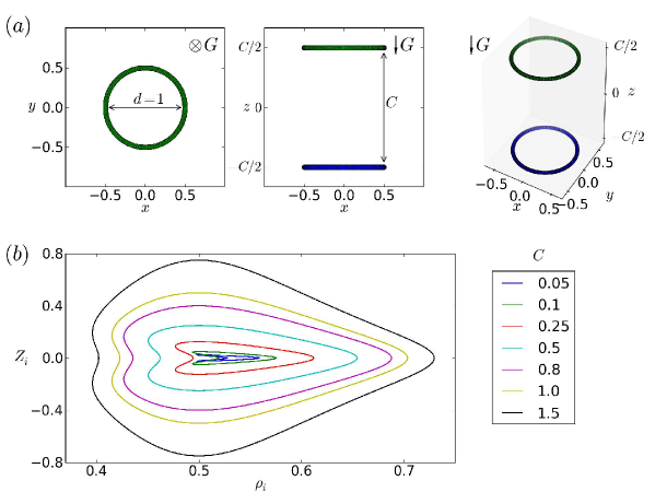
Figure 1: (Color online) The system of $M$ particles which form 2 rings. (a) $M\!=\!256$. The initial configuration as in Eq. (15). (b) $M\!=\!20000$. In the centre-of-mass frame, the trajectory of each particle has the same shape (not drawn to scale). Different shapes correspond to the indicated values of $C$.

Initially, the particles are placed at vertexes of $K$ horizontal regular polygons (called ’rings’) which are separated from each other vertically and centered one above (or below) the other. The diameter $d$ of the top ring is taken as the length unit. The number $N$ of particles in every ring is the same. Therefore, the total number of particles in the system is equal to $M=KN$. Because of the system symmetry, we use the cylindrical coordinate system, in which $\bm{r}_{i}$ is represented as $\bm{r}_{i}=(\rho_{i},\phi_{i},z_{i})$.

Searching for periodic solutions, we take into account that numerical non-symmetrical perturbations can destroy periodic unstable solutions after times smaller than the period, as observed in Ref. M. L. Ekiel-Jeżewska (2014). Therefore, we symmetrize the dynamics: we force the azimuthal components of the particle velocities to vanish, with $\phi_{i}\!=\!\text{const}(t)$ for $i\!=\!1,...,M$, and the polygons to remain regular for all times. We use the parametrization $i\!=\!K(n-1)+k$, with $n\!=\!1,...,N$ and $k\!=\!1,...,K$. Then,

$$\phi_{K(n-1)+k}=\frac{2\pi(n-1)}{N},$$ (8)

and the radial and vertical coordinates of the particles from the same polygon $k$ are the same,

$$\rho_{K(n-1)+k}\! = \!\rho_{k},$$ (9)

$$z_{K(n-1)+k}\! = \!z_{k},$$ (10)

for $n\!=\!1,...,N$ and $k\!=\!1,...,K$. The system of $3M$ equations (7) is reduced to the system of $2K$ equations for $\rho_{l}$ and $z_{l}$, with $l=1,...,K$, which in the frame of reference moving with the velocity $\mathbf{u}_{0}$ can be explicitly written as,

$$\frac{d\rho_{l}}{dt}\! = \!\!-\sum_{k=1}^{K}\sum_{n=1}^{N}\frac{(z_{k}-z_{l})\left[\rho_{k}\cos\left(\frac{2\pi(n-1)}{N}\right)-\rho_{l}\right]}{R_{lkn}^{3}},$$ (11)

$$\frac{dz_{l}}{dt}\! = \!\!-\sum_{k=1}^{K}\sum_{n=1}^{N}\left(\frac{1}{R_{lkn}}+\frac{(z_{k}-z_{l})^{2}}{R_{lkn}^{3}}\right),$$ (12)

$$\!\!R_{kln}^{2}\!\! = \!(z_{k}-z_{l})^{2}+\rho_{l}^{2}+\rho_{k}^{2}-2\rho_{l}\rho_{k}\cos\left(\!\frac{2\pi(n-1)}{N}\right)\!.\;$$

The numerical integration of Eqs. (11)-(LABEL:EOM3) is based on two methods: the fourth-order adaptive Runge-Kutta for non-stiff problems and backward differentiation formula (BDF) for stiff problems. We solve a system of ordinary differential equations using lsoda from the FORTRAN library odepack. Initially we start with non-stiff solver. Depending on number of time steps and accuracy the solver switches between method appropriate for stiff or non-stiff problem. This procedure is a standard and commonly used method for solving differential equations. This solver is sufficiently stable W. H. Press et al. (1992). The numerical calculations were performed with double precision and the error per each time step is not greater than $10^{-12}$.

We are interested in relative motion of the particles; therefore, we will trace their positions in the centre-of-mass frame of reference, located at the symmetry axis, $\bm{r}_{CM}=(0,0,z_{CM})$. In this frame, $\rho_{i}$ and $\phi_{i}$ are the same as in the laboratory frame, and particle vertical coordinates are $Z_{i}=z_{i}-z_{CM}$.

We perform simulations for two families of the systems: with two and four rings. The specific initial configurations and their evolution will be discussed in the next sections.

III Dynamics of 2 rings

We first consider a system of $M=2N$ particles which are grouped in two horizontal rings, each containing $N$ equally spaced particles. Initially, the rings are identical and placed one exactly above the other. The diameter of each ring is equal to $1$ and the initial distance $C$ between the rings is a parameter in our simulations, as shown in figure 1$(a)$. The initial positions $\bm{r}_{i}=(\rho_{i},\phi_{i},z_{i})$ of the particles $i=1,...,M$ are

$$\bm{r}_{2n-1} = \left(\frac{1}{2},\frac{2\pi(n-1)}{N},\frac{C}{2}\right),$$ (14)

$$\bm{r}_{2n} = \left(\frac{1}{2},\frac{2\pi(n-1)}{N},-\frac{C}{2}\right),$$ (15)

with $n=1,...,N$. We conducted around 100 simulations for $M=256$ and $20000$ particles and different initial values of $C\in[0.05,2.5]$. For these values of the parameters, we observe periodic motion of the particles during the whole simulation time $t=5000$ (what corresponds to 300-2700 periods), see our movie 1 in movies .

In the centre-of-mass frame, two particles with the same angular coordinates move along the same trajectory. Its shape is the same for all the pairs, and it depends on $C$ as shown in figure 1$(b)$ for $M\!=\!20~{}000$. We found similar families of shapes for $M\!=\!256$, analogical to those reported by M. L. Ekiel-Jeżewska (2014) for $M\!=\!16$, and resembling periodic solutions for rigid rods, discussed by S. Jung et al. (2006) and M. Bukowicki et al. (2015).

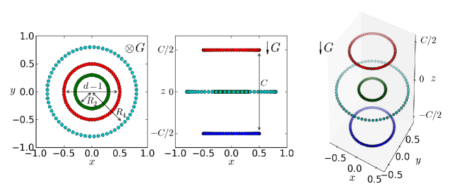
Figure 2: (Color online) Initially, $M$ particles form 4 rings, as specified in Eq. (19). Here, $M\!=\!256$.

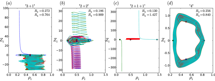
Figure 3: (Color online) Evolution of $M\!\!=\!\!256$ particles which form 4 rings with $C\!=\!1.5$ and $R_{2}$, $R_{4}$ as indicated. Trajectories of four particles (each from a different ring) in the centre-of-mass reference frame until time $t\!=\!500$. The initial positions are marked by dots. (a) ‘3+1’ type of decay. One of the rings separates from the cluster. (b) ‘2+2’ type of decay. The group breaks up into two pairs of oscillating rings - one of them falls faster than the other. (c) ‘2+1+1’ type of decay. The cluster breaks up into one pair of oscillating rings and two single rings. (d) ‘4’: lack of decay. All rings oscillate.

IV Dynamics of 4 rings

IV.1 Initial configurations

In the second system, $M=4N$ particles are grouped in four horizontal rings, each consisting of $N$ particles. Initially, the rings labeled $1$ and $3$ are placed at $z={C}/{2}$ and $-C/2$, respectively, and the rings labeled $2$ and $4$: at $z=0$, as shown in figure 2$(a)$. The radii of the rings $1,3,2$ and $4$ are equal to $1/2$, $1/2$, $R_{2}$, and $R_{4}$, respectively, with $R_{4}>R_{2}$. The angular coordinates of the particles from ring $1$ and ring $3$ are the same. The other rings are rotated by ${\pi}/{N}$ around the symmetry axis. Summarizing, the initial cylindrical coordinates of the particles are,

$$\bm{r}_{4n-3}\! = \!\left(\frac{1}{2},\frac{2\pi(n-1)}{N},\frac{C}{2}\right),$$ (16)

$$\bm{r}_{4n-2}\! = \!\left(R_{2},\frac{2\pi(n-\frac{1}{2})}{N},0\right),$$ (17)

$$\bm{r}_{4n-1}\! = \!\left(\frac{1}{2},\frac{2\pi(n-1)}{N},-\frac{C}{2}\right),$$ (18)

$$\bm{r}_{4n}\! = \!\left(R_{4},\,\frac{2\pi(n-\frac{1}{2})}{N},0\right),$$ (19)

where $n\!=\!1,...,N$ and $R_{2}$ and $R_{4}$ are the parameters of the simulation.

We performed around 400 000 simulations for clusters made of different numbers of particles $M\!=\!64,256,1024$ at the initial configurations specified by Eqs. (17)-(19), with $C\in[0.05,2.5]$, and a wide range of $R_{2}$ and $R_{4}$. In Secs. IV.2-IV.4 we will analyze how the dynamics depends on $R_{2}$ and $R_{4}$ for $M\!=\!256$ and $C\!=\!1.5$. Then, in Sec. IV.6, we will argue that these results are generic also for the other values of $M$ and $C$.

IV.2 Basic features of the dynamics

The dynamics of four rings of particles is more complex than the dynamics of two rings. Although the general pattern of oscillations combined with settling is kept, in case of four rings the motion in general is not periodic and we observe destabilisation and decay of the system, as in movie 2, see movies . Majority of initial conditions lead to the system decay during first $1000$ units of the simulation time, what corresponds to about $100$ oscillations.

If the group breaks up, usually one ring is left behind the other three or one ring falls faster than the rest of the group; we call it ‘3+1’ type of decay. If the system separates into two pairs of rings, we denote it ’2+2’ type of decay. We observe also ’2+1+1’ type of decay when two rings oscillate together and the others are separated. Examples of each decay type are presented in figure 3$(a)$-$(c)$ and movies 3a-c in movies .

For certain initial configurations, the particles perform quasiperiodic motion over a very long time. It has been checked that for several thousands of values of $R_{2}$ and $R_{4}$ the cluster lifetime exceeds $100000$. A typical shape of the corresponding trajectory $Z_{i}(\rho_{i})$ is shown in figure 3$(d)$ and movie 3d, see movies . These findings may indicate that for certain values of $R_{2}$ and $R_{4}$, periodic solutions exist, and they will be searched for later in this paper.

We would like to remind that all simulations are performed for symmetrized configurations and the particles by definition do not change the vertical planes they belong to, as described in Sec. II. The symmetrisation is done on purpose to find periodic solutions and ensure that the system will not break up because of non symmetrical numerical perturbations before a period is completed.

IV.3 Decay of the cluster

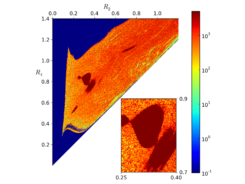
Figure 4: (Color) The cluster lifetime for around $420~{}000$ initial configurations with $C\!=\!1.5$ and different values of $R_{2}$ and $R_{4}$ (drawn to scale). The darkest red colour corresponds to the cluster lifetime larger than the simulation time $t\!=\!5000.$ Resolution of the map is $0.002\times 0.002$ and $M\!=\!256$.

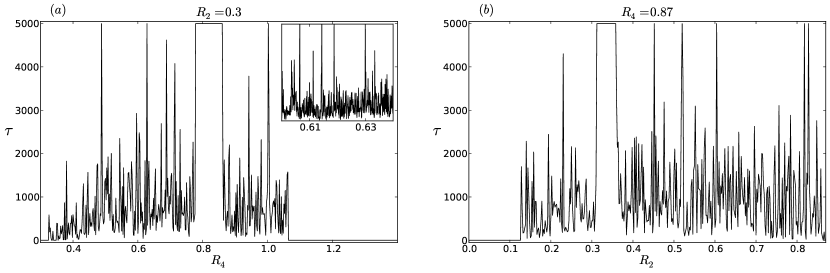
Figure 5: Cross-sections (now in the linear scale) through the map of the cluster lifetime from figure 4: (a) $R_{2}\!=\!0.3$, (b) $R_{4}\!=\!0.87$. Sensitivity to initial conditions is clearly visible. Inset: Scaling down the resolution of $R_{2}$ and $R_{4}$ from $0.002$ to $10^{-4}$, a self-similar structure is found.

To describe the system dynamics, it is crucial to define the event of the cluster decay and its time, denoted as $\tau$. The intrinsic property of a cluster of particles settling under gravity is the existence of periodic relative motions which may be used as an indicator whether the particles move together and interact with each other. For this reason we introduce a criterion of a cluster decay based on presence or absence of oscillations between pairs of particles. In particular, oscillations of particles $i$ and $j$ which belong to the same group imply that the difference of their $z$-coordinates, $\Delta z_{ij}=z_{i}-z_{j}$, oscillates around zero. We recognise that the particles $i,j$ interact and stay together if $\Delta z_{ij}$ has repeating roots.

Therefore, we use the following definition of the cluster decay. For each pair of particles $i,j$ we calculate the difference $\Delta z_{ij}$ of their $z$-coordinates as a function of time. If for any $l,m$ the time interval between two consecutive roots, $t_{A}$ and $t_{B}>t_{A}$, of $\Delta z_{lm}$ exceeds $1000$, we classify it as the cluster decay and denote $\min_{l,m}t_{A}$ as the cluster lifetime $\tau$.

This criterion of decay works well, in contrast to attempts based on measuring only the relative vertical distances between rings, because it is common that rings approach each other again, even though they were separated by a very long vertical distance meanwhile, as observed by M. L. Ekiel-Jeżewska & E. Wajnryb (2011) for systems of three particles.

To define the type of the cluster decay we apply the following procedure: we count the number of roots of $\Delta z_{ij}$ in the time interval $[\tau,\mbox{min}(\tau+1000,T)]$ for each pair of particles $ij$. If the number of roots is smaller than the length of the time interval divided by $200$ (for the interval $[\tau,\tau+1000]$ it is equal to $5$), we define that the particles $i,j$ interact with each other. Otherwise, we denote them as separated. The number $L$ of interacting pairs indicates the type of the decay. $L\!=\!3$ corresponds to ‘3+1’ type of the decay, $L\!=\!2$ to ‘2+2’ type of the decay, $L\!=\!1$ to ‘2+1+1’ type of the decay and $L\!=\!0$ to ‘1+1+1+1’. For $L\!=\!6$ there is no decay (type ‘4’).

Now, the main question is how the lifetime depends on initial conditions. The results are presented in figure 4 as a map in space of the parameters $R_{2}$ and $R_{4}$, with colours indicating the logarithm of the cluster lifetime. Values of $(R_{2},R_{4})$ which lead to long-living clusters form a few compact regions, around which only isolated configurations with long lifetimes can be found. Deterministic regions are visible when $R_{2}$ is small enough, or $R_{4}$ is large enough, and the cluster splits up immediately without oscillations. In the first case, settling velocity of a very small ring 2 is much larger than velocities of the other rings, while in the second case, settling velocity of a very large ring 4 is much smaller than velocities of the other rings.

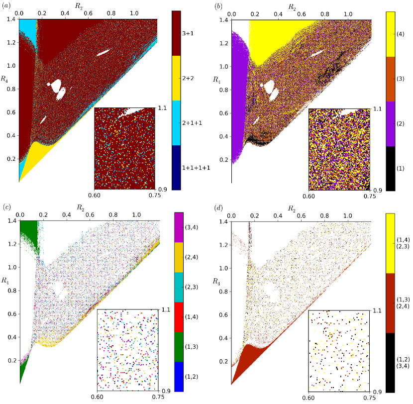
Figure 6: (Color) Sensitivity of patterns of the cluster decay to the initial parameters $R_{2}$ and $R_{4}$, for $C\!=\!1.5$ and $M\!=\!256$. White colour means no decay. (a) The types of the decay: into ‘3+1’, ‘2+2’, ‘2+1+1’ or ‘1+1+1+1’ rings (see Sec. IV.3 for the exact definitions). (b) ‘3+1’ type of the decay: the colour indicates the label of the ring which separates from the others at time $\tau$. (c) ‘2+1+1’ type of the decay: the colours indicate the interacting pair of the rings at time $\tau$. (d) ‘2+2’ type of the decay: the colours indicate which rings form interacting pairs at time $\tau$.

The essential property of the map shown in figure 4 is that for a wide range of $R_{2}$ and $R_{4}$, the cluster lifetime is very sensitive to initial conditions. Around the regions of long-living clusters (with very sharp edges) we find a variability of the cluster lifetime by orders of magnitude. This property is also well visible in figure 5 at the cross sections of the map, plotted in the linear scale. This behaviour is similar to the chaotic scattering reported by I. M. Janosi et al. (1997) for three point particles sedimenting in a vertical plane.

In figure 6, we show the type of the cluster decay and labels of the particles which interact with each other at the decay time $\tau$, depending on $R_{2}$ and $R_{4}$. Sensitivity to initial conditions is clearly visible at most of the map areas, except a few deterministic regions corresponding to a very long or very short lifetimes. The last ones can be easily understood by comparing the ring diameters, and taking into account that the smaller the ring, the larger is its velocity.

IV.4 Clusters with long lifetimes and quasiperiodic solutions

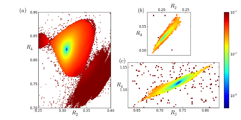
Figure 7: (Color) The average deviation $\Delta$ of particle trajectories for clusters with lifetimes $\tau\geq 5000$, $C\!=\!1.5$ and $M\!=\!256$. Resolution: $(a)$: 0.001 $\times$ 0.001; $(b)$ and $(c)$: 0.002 $\times$ 0.002. The minima at the subplots (a),(b),(c) correspond to the solutions presented in Fig.8(a),(b),(c), respectively.

We have found that the long lifespan of the cluster and quasiperiodic trajectories of particles are observed for the system with initial configurations grouped in a few regions (see figure 4). We will now investigate trajectories from each of the specific long-lifetime regions, and search for periodic solutions.

To this goal, we apply the Dynamic Time Warping (DTW) method, described e. g. by M. Müller (2007) and M. Vlachos et al. (2002). For each particle $i$, we define its reference trajectory $Z^{r}_{i}(\rho_{i})$ for times $t_{1}\!\leq\!t\!\leq\!t_{3}$, where $t_{k}$, $k\!=\!1,2,3$, are the first, second and third time instants when $Z_{i}(t_{k})\!=\!0$. Then, for $t_{3}\!\leq\!t\!\leq\!5000$, we calculate the Euclidean distance $d_{i}(t)$ between the particle position $(Z_{i}(t),\rho_{i}(t))$ and its reference trajectory. We define the average deviation $\Delta$ of the trajectories as the average of $d_{i}(t)$ over all the particles $i$ and all times $t$.

In figure 4, we surround three main long-lifetime islands in the $R_{2}$-$R_{4}$ space by rectangular boxes of a fixed resolution, and evaluate for each pixel the average deviation $\Delta$ of the trajectories. The results are shown in figure 7. For each of the three boxes, there exists a smallest deviation $\Delta_{\text{min}}$, corresponding to a very thin trajectory. For example, in figure 7$(a)$, $\Delta_{\text{min}}\!=\!3\cdot 10^{-4}$ is three hundred times smaller than deviation of the quasiperiodic trajectories shown in figure 3$(d)$.

IV.5 Three periodic solutions

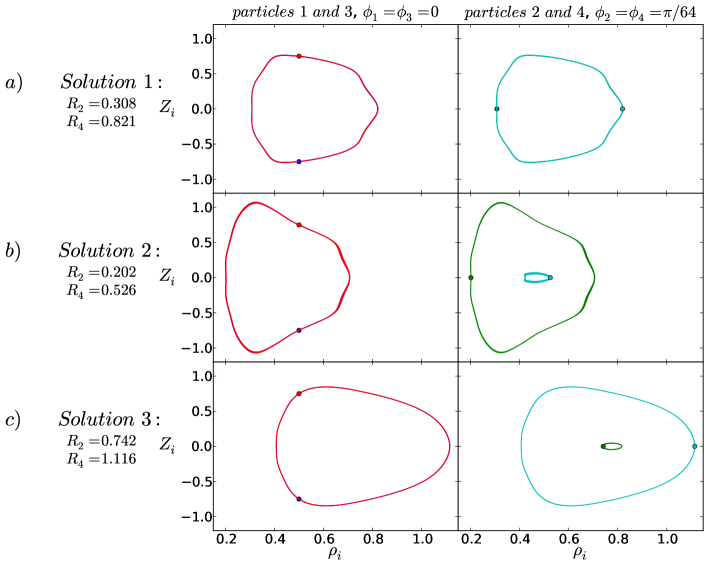
Figure 8: (Color online) Periodic trajectories of four particles (each from a different ring) in the centre of mass frame of a cluster with $M\!=\!256$ particles. Dots: the initial particle positions, with $C\!=\!1.5$. Solutions in the subplots (a)-(c) correspond to the minima of $\Delta$ in Figs. 7(a)-(c), respectively.

The minima visible in figures 7$(a)$,$(b)$,$(c)$ correspond to three periodic trajectories in the centre-of-mass frame of the cluster, shown in figures 8$(a)$,$(b)$,$(c)$, respectively. We remind that owing to the symmetrization of the dynamics, each particle from ring $i$ has the same coordinates $Z_{i}(t)$ and $\rho_{i}(t)$. Therefore, it is sufficient to display $Z_{i}(\rho_{i})$ for particles $i\!=\!1,2,3,4$: each from a different ring $i$, with particles $1,3$ moving in vertical plane $\phi\!=\!0$ and particles $2,4$ moving in another vertical plane $\phi\!=\!4\pi/M$. Here, $M\!=\!256$ and $C\!=\!1.5$.

The new periodic solutions have the following properties.

Solution 1, shown in figure 8(a) and movie 8a in movies , is located in the middle of the biggest of the long-lifetime regions from figure 4, and at the minimum of the trajectories deviation $\Delta$ in Fig. 7(a). All four particles move along the same trajectory $Z_{i}(\rho_{i})$, shifted in phase by $T/4$, with the period $T=11.7$.

Solution 2, shown in figure 8(b) and movie 8b in movies , is located in the middle of a small long-lifetime region from figure 4, and at the minimum of the trajectories deviation $\Delta$ in Fig. 7(b). It corresponds to the initial radius $R_{2}$ of the ring 2 much smaller than the initial radius of the rings 1 and 3, $R_{1}\!=\!R_{3}\!=\!0.5$, and with $R_{4}\!\gtrsim\!0.5$. The central particle 4 has its own tiny trajectory and is circulated by the other three, which move along a larger trajectory with the period $T\!=\!10.7$, shifted in phase by $T/3$ with respect to each other. The period of particle 4 is equal to $T/3$.

Solution 3, shown in figure 8(c) and movie 8c in movies , is located in the middle of the other small long-lifetime region from figure 4, and at the minimum of the trajectories deviation $\Delta$ in Fig. 7(c). The corresponding initial configuration satisfies the relations, $R_{2},R_{4}>R_{1}\!=\!R_{3}\!=\!0.5$. Now particle 2 is the central one, and the motion is qualitatively similar to solution 2, with the interchange of the particles 2 and 4, and much wider rings, what leads to a larger period, $T=15.6$, because larger rings move slower.

IV.6 Two families of periodic solutions

Periodic oscillations have been found for many values of $C$. In figure 9 we show how the shape of the periodic trajectory of type 1 depends on $C$. Periodic solutions 1, 2 and 3 for $C\!=\!2$ are shown in figure 10 in the Appendix. These examples illustrate that the basic properties of the periodic solutions, described in the previous section and shown in figure 8, are generic for a wide range of values of $C$.

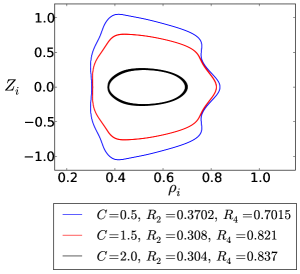
Figure 9: (Color online) Periodic solutions of type 1 for different values of $C$ and $M\!=\!256$.

Initially, two particles are at the same horizontal plane, and the other two particles are exactly one above the other. Movies 8b,c in movies illustrate that for each periodic solution 2 or 3, such a configuration appears again at $T/6$, but with different values of $C$, $R_{2}$ and $R_{4}$, which correspond to solutions 3 or 2, respectively. This new configuration can be treated as another initial condition for the same periodic solution. Therefore, assuming that there exist periodic solutions for all sufficiently large values of $C$, we predict the existence of twin solutions 2 and 3 for each value of $C$ which is large enough.

Dynamics of 4 rings made of other numbers $M\!=\!64,1024$ of the particles have been also evaluated, and similar families of periodic solutions have been found.

V Discussion and concluding remarks

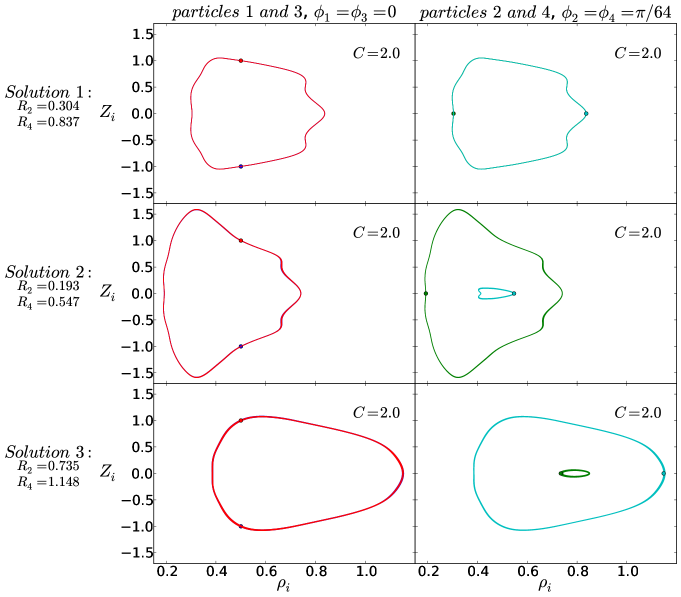
Figure 10: (Color online) Periodic trajectories of four particles (each from a different ring) in the centre of mass frame of a cluster with $M\/=\/256$ particles. Dots: the initial particles positions. Here, $C\/=\/2.0$ (compare with figure 8 where $C\/=\/1.5$).

In this work, we searched for periodic relative motions of many particles which form regular clusters with aspect ratios of the order of one. We generalized in this way the previous solutions found in Ref. M. L. Ekiel-Jeżewska (2014) for a smaller number of particles. In Ref. M. L. Ekiel-Jeżewska (2014), the systems of 2 rings were shown to destabilize. Therefore, to determine accurately periodic motions, in this paper we solved the symmetrized dynamics, given in Eqs. (11)-(LABEL:EOM3). Although we have not analyzed here the non-symmetric perturbations, but it is known from Ref. M. L. Ekiel-Jeżewska (2014) that such perturbations destabilize the system after times which are large enough to observe the existence of periodic solutions and determine the cluster lifetimes (e. g. for 64 particles, periodic motions destablize at times $t$ not shorter than half of the period, $T/2$, while even the motion during $T/4$ would be sufficient to deduce the existence of unstable periodic solutions).

A similar behaviour was observed experimentally in Ref. J. Nowakowskiet al. (2014) for three close particles sedimenting approximately in a vertical plane. Typically, periodic motions have been observed during times comparable to one sixth of the period, $T/6$. Owing to symmetries of the motion, this is sufficient to demonstrate the existence of unstable periodic orbits. Moreover, in these experiments, the same type of periodic orbit was reached again after the destabilization, and this pattern of approaching and leaving the periodic orbit was repeated several times. Summarizing, examples of unstable periodic motions can be easily observed in experiments, and sometimes unstable periodic motions form a generic feature of the dynamics.

In this work, we found a surprisingly large number of periodic solutions. For a cluster made of 2 rings, they were observed for all the investigated shapes (parameterized by moderate values of the initial aspect ratio $C$), and particle numbers $N$ even as large as 20 000.

It has been interesting to modify the initial 2-rings configuration, with particles arranged in 4 rings, and in this way desynchronized. It turned out that clusters made of 4 rings usually break up, and their lifetime and type of decay are in general sensitive to initial conditions. In the 2D space of initial parameters, the deterministic area surrounds the chaotic region. The last one contains islands of quasiperiodic oscillations which do not destabilize during extremely long simulation times. At the centers of these islands, three different periodic solutions exist, parameterized by the initial cluster height and the number of particles.

The results provide a new perspective for the physical mechanism of decay of particle clusters sedimenting in a viscous fluid, typically with a very wide range of life times.

Appendix A Periodic trajectories for a different value of the parameter $C$

In this Appendix, we illustrate that Fig. 8 with $C=1.5$ provides a generic example of two families of periodic solutions: solution 1 corresponds to the first family, and the solutions 2 and 3 to the second family, as discussed in Sec. IV.6. Such a structure of the periodic solutions has been observed for many values of the parameter $C$, which determines the initial geometry of the upper and lower rings. In Fig. 10, we show another example: the periodic orbits for $C=2$ (compare with Fig. 8).

References

- (1) G. Jeffery, Proc. R. Soc. 102, 161 (1922).
- (2) M. Reichert & H. Stark, J. Phys.: Condens. Matter 16, S4085 (1991)
- (3) C. Lutz, M. Reichert, H. Stark & C. Bechinger, Europhys. Lett. 74 719 (2006).
- (4) Y. Roichman, D. G. Grier & G. Zaslavsky, Phys. Rev. E 75, 020401(R) (2007)
- (5) Y. Sokolov, D. Frydel, D. G. Grier, H. Diamant & Y. Roichman, Phys. Rev. Lett. 107, 158302 (2011)
- (6) Y. Sassa, S. Shibata, Y. Iwashita & Y. Kimura, Phys. Rev. E 85, 061402 (2012)
- K. O. L. F. Jayaweera et al. (1964) K. O. L. F. Jayaweera, B. J. Mason & H. W. Slack, J. Fluid Mech. 20, 121-128 (1964)
- (8) B. H. Kaye, Ph. D. Thesis, London Univ. (1961)
- (9) B. Koglin, Chemie Ingenieur Technik 44, 515(1972).
- (10) B. Koglin, Habilitation Thesis, Karlsruhe Univ. (1973).
- (11) B. Koglin and A. Al-Taweel, in: Harold Haywood Memorial Symposium, Loughborough: University of Technology (1973).
- (12) B. Koglin, A. Al-Taweel and N. Ahmad, Chemie Ingenieur Technik 48. 557 (1976).
- (13) S. Alabrudziński S., M. L. Ekiel-Jeżewska, D. Chehata-Gomez, T. A. Kowalewski, Phys. Fluids, 21, 73302 (2009).
-
J. Nowakowskiet al. (2014)
J. Nowakowski & M. L. Ekiel-Jeżewska, Gallery of Fluid Motion 2014,
http://dx.doi.org/10.1103/APS.DFD.2014.GFM.P0061 - L. M. Hocking (1963) L. M. Hocking, J. Fluid Mech. 20, 129-139 (1963)
- L. Durlofskyet al. (1987) L. Durlofsky & J. F. Brady, J. Fluid Mech. 180, 21-49 (1987)
- R. E. Caflisch et al. (1988) R. E. Caflisch, C. Lim, J. H. C. Luke & A. S. Sangani, Phys. Fluids 31, 3175 (1988)
- M. T. Kamelet al. (1990) M. T. Kamel & E. M. Tory, Powder Technol. 63, 187-195 (1990)
- E. M. Tory et al. (1991) E. M. Tory, M. T. Kamel & C. B. Tory, Powder Technol. 67, 71–82 (1991)
- M. Golubitskyet al. (1991) M. Golubitsky, M. Krupa & Ch. Lim, SIAM J. Appl. Math. 51, 1 (1991)
- E. M. Toryet al. (1992) E. M. Tory & M. T. Kamel, Powder Technol. 73, 95-96 (1992)
- Ch. C. Limet al. (1995) Ch. C. Lim & I. H. McMomb, J. Differ. Equations 121, 2 (1995)
- I. K. Snooket al. (1997) I. K. Snook, K. M. Briggs & E. R. Smith, Physica A 240, 547–559 (1997)
- M. L. Ekiel-Jeżewska, T. Gubiec & P. Szymczak (2008) M. L. Ekiel-Jeżewska, T. Gubiec & P. Szymczak, Phys. Fluids 20, 63102 (2008)
- M. Bargiełet al. (2011) M. Bargieł, M. T. Kamel & E. M. Tory, Powder Technol. 214, 14-20 (2011)
- M. Bargiełet al. (2014) M. Bargieł & E. M. Tory, Powder Technol. 264, 519-526 (2014)
- I. M. Janosi et al. (1997) I. M. Janosi, T. Tel, D. E. Wolf & J. A. C. Gallas, Phys. Rev. E. 56, 2858-2868 (1997)
- M. L. Ekiel-Jeżewska & E. Wajnryb (2011) M. L. Ekiel-Jeżewska & E. Wajnryb, Phys. Rev. E 83, 067301 (2011)
- M. L. Ekiel-Jeżewska (2008) M. L. Ekiel-Jeżewska, CDROM Proceedings of the XXII International Congress of Theoretical and Applied Mechanics, edited by J. Denier, M. D. Find and T. Mattner, University of Adelaide; ISBN: 978-0-9805142-1-6 (2008)
- (30) J. M. Nitsche, G. K. Batchelor, J. Fluid Mech. 340, 161 (1997).
- A. Myłyk et al. (2011) A. Myłyk, W. Meile, G. Brenn & M. L. Ekiel-Jeżewska, Phys. Fluids. 23, 063302 (2011)
- M. L. Ekiel-Jeżewska (2014) M. L. Ekiel-Jeżewska, Phys. Rev. E 90, 043007 (2014)
- S. Jung et al. (2006) S. Jung, S. E. Spagnolie, K. Parikh, M. Shelley & A. K. Tornberg, Phys. Rev. E. 74, 035302(R) (2006)
- S. Kim & S. J. Karrila (2005) S. Kim & S. J. Karrila, Microhydrodynamics. Principles and Selected Applications, Dover Publications, Inc., New York (2005)
- W. H. Press et al. (1992) W. H. Press, S. A. Teukolsky, W. T. Vetterling & B. P. Flannery, Numerical Recipes in FORTRAN. The Art of Scientific Computing, Cambridge University Press, 1992, pp. 727-731.
- (36) See Supplemental Material at [URL will be inserted by publisher] for the movies and their description.
- M. Bukowicki et al. (2015) M. Bukowicki, M. Gruca & M. L. Ekiel-Jeżewska, J. Fluid Mech. 767, 95-108 (2015).
- M. Müller (2007) M. Müller, Information Retrieval for Music and Motion, Springer-Verlag, Berlin Heidelberg (2007).
- M. Vlachos et al. (2002) M. Vlachos, G. Kollios & D. Gunopulos, Proceedings of the 18th International Conference on Data Engineering, pp. 673-684 (2002)