Abstract

In this note we aim to infer a model for the response of a Pierre Auger water-Cherenkov detector to an ideal single muon. The main goal of this analysis is to provide analytical support for muon counting techniques. In this note we derive the probability distribution of the muon tracklength as a function of the zenith angle of the muon.

1 Introduction

This note is the first in a series of notes in which we aim to infer a model for the response of a Pierre Auger water Cherenkov detector (tank from now on) to an ideal single muon. The single muon response is a subject that was thoroughly explored in the early phase of the Auger collaboration [1, 2, 3, 4, 5, 6, 7, 8, 9, 10, 11, 12, 13, 14, 15, 16]. The main purpose of these studies was to understand the mean muon response (more precisely, the so-called muonic peak or the “muon hump”) in order to define an SD energy estimate. First, based on the muonic peak model, a calibration procedure was designed for estimating the total signal in individual tanks. Then the total signals were combined to compute one observable per shower, which was finally calibrated to the energy estimate of the fluorescence detector (FD).

Since the SD energy estimate is calibrated to the FD energy estimate, the procedure is relatively robust against systematic biases of the mean muon response estimate as long as the biases are stable among different tanks and not changing with time. The fluctuations of the muonic signal are also not too important from the point of view of the energy estimation. On the other hand, the goal of muon-counting [17, 18, 19, 20] is to design a muon density estimator without the need for outside calibration. Now biases due to the tank geometry and the energy-dependence of the muonic response become important. Furthermore, since these techniques are based on certain statistics of the individual muonic “jumps”, understanding the fluctuations of the muon response is of great importance. Our ultimate goal is similar to the program outlined in [12]: obtain a full parametrization of the muonic signal that can be used in a Monte Carlo Markov chain [21] reconstruction approach as well as for fine-tuning the muon counting techniques. Beside this principal goal, we believe that this refined model may also help to improve the SD energy estimate (mainly by decreasing the statistical error on the individual shower estimates along the lines of [22]). The obtained model may also serve as a basis for a toy Monte-Carlo tank simulator that can be used to quickly generate a large number of tank signals.

1.1 Introduction to this note

In a crude model, the total muonic signal is proportional to the tracklength of the muon in the water tank, so the fluctuation of the tracklength at a given zenith angle is the main source of the fluctuation of the total muonic signal. In this note we derive the tracklength distribution $\raisebox{-1.72218pt}{\leavevmode\resizebox{}{6.02773pt}{$\mathcal{P}$}}_{L}(L\mid\theta)$ of a muon that crosses the tank at zenith angle $\theta$. Most of the formulas can also be found in [11]. Our main contribution is that we give clean formulas that can be used directly in a probabilistic generative model. We also add one term for muons that enter and leave at the lateral of the tank. This part of the signal, which was omitted by [11], may be important for inclined showers.

2 The distribution of the muon tracklength

In this section we derive the tracklength distribution $\raisebox{-1.72218pt}{\leavevmode\resizebox{}{6.02773pt}{$\mathcal{P}$}}_{L}(L\mid\theta)$ of a muon that crosses the tank zenith angle $\theta$. To transform the quantities into unit-less variables, we first apply the substitutions

$$\ell=\frac{L}{2R}\qquad\text{and}\qquad h=\frac{H}{2R},$$ (1)

where $h=1/3$ for an Auger tank with height $H=1.2\,\mathrm{m}$ and radius $R=1.8\,\mathrm{m}$. From now on we will only derive the distribution $\raisebox{-1.72218pt}{\leavevmode\resizebox{}{6.02773pt}{$\mathcal{P}$}}(\ell\mid\theta)$ as a function of the unit-less variable $\ell$. The original distribution in $L$ can be recovered by the transformation

$$\raisebox{-1.72218pt}{\leavevmode\resizebox{}{6.02773pt}{$\mathcal{P}$}}_{L}(L\mid\theta)=\frac{1}{2R}\raisebox{-1.72218pt}{\leavevmode\resizebox{}{6.02773pt}{$\mathcal{P}$}}(L/2R\mid\theta).$$ (2)

The distribution can be decomposed into three components: the lid–base (lb) term of the form $\raisebox{-1.72218pt}{\leavevmode\resizebox{}{6.02773pt}{$\mathcal{P}$}}_{\text{lb}}(\ell\mid\theta)\,\mathcal{P}(\text{lb}\mid\theta)$ representing muons entering at the lid of the tank and leaving at the base, the lid–lateral (li) term $\raisebox{-1.72218pt}{\leavevmode\resizebox{}{6.02773pt}{$\mathcal{P}$}}_{\text{li}}(\ell\mid\theta)\,\mathcal{P}(\text{li}\mid\theta)$ representing muons entering at the lid and leaving at the lateral (or, symmetrically, entering at the lateral and leaving at the base), and the lateral–lateral (la) term $\raisebox{-1.72218pt}{\leavevmode\resizebox{}{6.02773pt}{$\mathcal{P}$}}_{\text{la}}(\ell\mid\theta)\,\mathcal{P}(\text{la}\mid\theta)$ representing muons entering and leaving at the lateral (for these regions see projected tank schematic in Fig. 1). We have thus

$$\raisebox{-1.72218pt}{\leavevmode\resizebox{}{6.02773pt}{$\mathcal{P}$}}(\ell\mid\theta)=\raisebox{-1.72218pt}{\leavevmode\resizebox{}{6.02773pt}{$\mathcal{P}$}}_{\text{lb}}(\ell\mid\theta)\,\mathcal{P}(\text{lb}\mid\theta)+\raisebox{-1.72218pt}{\leavevmode\resizebox{}{6.02773pt}{$\mathcal{P}$}}_{\text{li}}(\ell\mid\theta)\,\mathcal{P}(\text{li}\mid\theta)+\raisebox{-1.72218pt}{\leavevmode\resizebox{}{6.02773pt}{$\mathcal{P}$}}_{\text{la}}(\ell\mid\theta)\,\mathcal{P}(\text{la}\mid\theta).$$ (3)

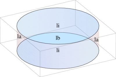
Figure 1: Projection of the Auger tank along the incoming muon direction at $\theta=50^{\circ}$. The three components of the tracklength distribution $\raisebox{-1.72218pt}{\leavevmode\resizebox{}{6.02773pt}{$\mathcal{P}$}}(\ell\mid 50^{\circ})$ are visible: the lid–base (lb), the lid–lateral (li), and the lateral–lateral (la) terms.

2.1 Case probabilities

We proceed by first computing the case probabilities $\mathcal{P}(\text{lb}\mid\theta)$, $\mathcal{P}(\text{li}\mid\theta)$, and $\mathcal{P}(\text{la}\mid\theta)$. First we need the area $A(\theta)$ of the tank projection for zenith angle $\theta$,

$$A(\theta)=\pi R^{2}|\cos\theta|+2RH\sin\theta.$$ (4)

Note that the absolute value is used in order to render the equations useful also for cases when muons are entering the tank with zenith angle $\theta$ larger than $90^{\circ}$ (i.e., useful for albedo studies). Measuring area in units of the top surface $A_{\text{t}}=\pi R^{2}$ and using the unit-less $h$, we can define

$$a(\theta)=\frac{A(\theta)}{A_{\text{t}}}=|\cos\theta|+\tfrac{4}{\pi}h\sin\theta=\tfrac{2}{\pi}|\cos\theta|(\tfrac{\pi}{2}+2u),$$ (5)

where

$$u=h|\tan\theta|.$$ (6)

Measuring the partial areas (see Fig. 3(a)) in the same relative unit $a_{\text{xx}}=A_{\text{xx}}/A_{\text{t}}$, we obtain for the lid–base part

$$a_{\text{lb}}(\theta) =\begin{cases}\tfrac{2}{\pi}\left(|\cos\theta|\arccos(h\tan\theta)-h\sin\theta\sqrt{1-(h\tan\theta)^{2}}\right)&\text{ if $|\tan\theta|\leqslant 1/h$,}\\[11.38109pt] 0&\text{ otherwise,}\end{cases}$$ (7)

$$=\tfrac{2}{\pi}|\cos\theta|\begin{cases}\arccos u-u\sqrt{1-u^{2}}&\text{ if $u\leqslant 1$,}\\[11.38109pt] 0&\text{ otherwise,}\end{cases}$$ (8)

for the lid–lateral part

$$a_{\text{li}}(\theta) =2\big{(}|\cos\theta|-a_{\text{lb}}(\theta)\big{)}=$$ (9)

$$=\tfrac{4}{\pi}|\cos\theta|\begin{cases}\arcsin u+u\sqrt{1-u^{2}}&\text{ if $u\leqslant 1$,}\\[11.38109pt] \tfrac{\pi}{2}&\text{ otherwise,}\end{cases}$$ (10)

and for the lateral–lateral part

$$a_{\text{la}}(\theta) =\tfrac{4}{\pi}h\sin\theta-|\cos\theta|+a_{\text{lb}}(\theta)=$$ (11)

$$=\tfrac{2}{\pi}|\cos\theta|\begin{cases}2u-\arcsin u-u\sqrt{1-u^{2}}&\text{ if $u\leqslant 1$,}\\[11.38109pt] 2u-\tfrac{\pi}{2}&\text{ otherwise.}\end{cases}$$ (12)

The case probabilities (see Fig. 3(b)) are then given by

$$\mathcal{P}(\text{lb}\mid\theta)=\frac{a_{\text{lb}}(\theta)}{a(\theta)},\qquad\mathcal{P}(\text{li}\mid\theta)=\frac{a_{\text{li}}(\theta)}{a(\theta)},\quad\text{and}\quad\mathcal{P}(\text{la}\mid\theta)=\frac{a_{\text{la}}(\theta)}{a(\theta)}.$$ (13)

Note that for the final case probabilities, the $2|\cos\theta|/\pi$ term cancels in this process.

2.2 Probability distribution functions

The lid–base term $\raisebox{-1.72218pt}{\leavevmode\resizebox{}{6.02773pt}{$\mathcal{P}$}}_{\text{lb}}(\ell\mid\theta)$ is a simple Dirac delta

$$\raisebox{-1.72218pt}{\leavevmode\resizebox{}{6.02773pt}{$\mathcal{P}$}}_{\text{lb}}(\ell\mid\theta)=\delta(\ell-\ell_{\text{max}}),$$ (14)

where $\ell_{\text{max}}(\theta)$ is the maximum tracklength (see Fig. 2) defined as

$$\ell_{\text{max}}(\theta)=\begin{cases}h/|\cos\theta|&\text{ if $|\tan\theta|\leqslant 1/h$},\\ 1/\sin\theta&\text{ otherwise.}\end{cases}$$ (15)

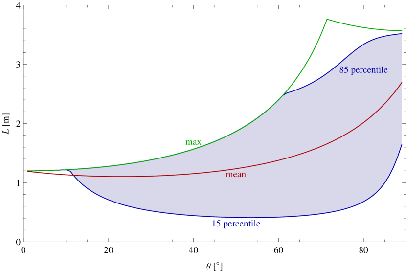
Figure 2: The mean tracklength $\bar{L}(\theta)={{\mathbb{E}}\left\{{\raisebox{-1.72218pt}{\leavevmode\resizebox{}{6.02773pt}{$\mathcal{P}$}}_{L}(L|\theta)}\right\}}$ (red), the maximum tracklength $L_{\text{max}}(\theta)=2R\ell_{\text{max}}(\theta)$ (green), and the region that contains $70\%$ of the probability mass (blue) as a function of the zenith angle $\theta$.

Note that the case $1/\sin\theta$ is never in effect in the lid–base term since the case probability $\mathcal{P}(\text{lb}|\theta)$ is zero in this range. The lid–lateral and lateral–lateral terms are

$$\raisebox{-1.72218pt}{\leavevmode\resizebox{}{6.02773pt}{$\mathcal{P}$}}_{\text{li}}(\ell\mid\theta) =\frac{1}{a_{\text{li}}(\theta)}\begin{cases}\tfrac{4}{\pi}|\sin 2\theta|\sqrt{1-(\ell\sin\theta)^{2}}&\text{ if $0\leqslant\ell\leqslant\ell_{\text{max}}(\theta)$,}\\[11.38109pt] 0&\text{ otherwise,}\end{cases}$$ (16)

$$\raisebox{-1.72218pt}{\leavevmode\resizebox{}{6.02773pt}{$\mathcal{P}$}}_{\text{la}}(\ell\mid\theta) =\frac{1}{a_{\text{la}}(\theta)}\begin{cases}\displaystyle\tfrac{4}{\pi}\frac{\ell\sin^{3}\theta(h-\ell|\cos\theta|)}{\sqrt{1-(\ell\sin\theta)^{2}}}&\text{ if $0\leqslant\ell\leqslant\ell_{\text{max}}(\theta)$,}\\[11.38109pt] 0&\text{ otherwise,}\end{cases}$$ (17)

respectively.

2.3 Cumulative distribution functions

The cumulative distribution functions of the continuous terms are

$$\int_{0}^{\ell}\!\raisebox{-1.72218pt}{\leavevmode\resizebox{}{6.02773pt}{$\mathcal{P}$}}_{\text{li}}(\ell^{\prime}\mid\theta)\,{\rm d}\ell^{\prime} =\tfrac{4}{\pi}\frac{|\cos\theta|}{a_{\text{li}}(\theta)}\left[\arcsin(\ell\sin\theta)+\ell\sin\theta\sqrt{1-(\ell\sin\theta)^{2}}\right]=$$ (18)

$$=\begin{cases}\displaystyle\frac{\arcsin v+v\sqrt{1-v^{2}}}{\arcsin u+u\sqrt{1-u^{2}}}&\text{ if $u\leqslant 1$,}\\[11.38109pt] \displaystyle\frac{\arcsin v+v\sqrt{1-v^{2}}}{\pi/2}&\text{ otherwise,}\end{cases}$$ (19)

$$\int_{0}^{\ell}\!\raisebox{-1.72218pt}{\leavevmode\resizebox{}{6.02773pt}{$\mathcal{P}$}}_{\text{la}}(\ell^{\prime}\mid\theta)\,{\rm d}\ell^{\prime} =$$ (20)

$$\tfrac{2}{\pi}\frac{|\cos\theta|}{a_{\text{la}}(\theta)} \left[2h|\tan\theta|-\arcsin(\ell\sin\theta)-\left(2h|\tan\theta|-\ell\sin\theta\right)\sqrt{1-(\ell\sin\theta)^{2}}\right]=$$ (21)

$$=\begin{cases}\displaystyle\frac{2u-\arcsin v-(2u-v)\sqrt{1-v^{2}}}{2u-\arcsin u-u\sqrt{1-u^{2}}}&\text{ if $u\leqslant 1$,}\\[11.38109pt] \displaystyle\frac{2u-\arcsin v-(2u-v)\sqrt{1-v^{2}}}{2u-\pi/2}&\text{ otherwise,}\end{cases}$$ (22)

where

$$v=\ell\sin\theta,$$ (23)

and the full cumulative distribution is

$$\int_{0}^{\ell}\!\raisebox{-1.72218pt}{\leavevmode\resizebox{}{6.02773pt}{$\mathcal{P}$}}(\ell^{\prime}\mid\theta)\,{\rm d}\ell^{\prime}=\begin{cases}\displaystyle\frac{\arcsin v+2u+(3v-2u)\sqrt{1-v^{2}}}{2u+\pi/2}&\text{ if $v\leqslant\min(1,u)$,}\\[11.38109pt] 1&\text{ otherwise.}\end{cases}$$ (24)

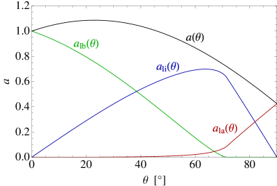
(a) relative areas

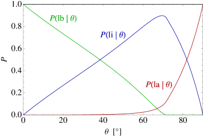
(b) case probabilities

Figure 3: (a) The relative partial areas $a_{\text{lb}}(\theta)$, $a_{\text{li}}(\theta)$, $a_{\text{la}}(\theta)$, and their sum $a(\theta)$, and (b) the case probabilities $\mathcal{P}(\text{lb}\mid\theta)$, $\mathcal{P}(\text{li}\mid\theta)$, and $\mathcal{P}(\text{la}\mid\theta)$ as a function of the zenith angle $\theta$.

2.4 Mean tracklength

It has already been noted several times that the mean tracklength $\bar{L}(\theta)$ (see Fig. 2) for muons arriving with a specific zenith angle $\theta$ is quite easy to obtain without integrating $L\raisebox{-1.72218pt}{\leavevmode\resizebox{}{6.02773pt}{$\mathcal{P}$}}_{L}(L\mid\theta)$. If we enlarge the puncturing track of a muon so that it has the same cross section ${\rm d}A$ along the path, a small volume ${\rm d}V$ is obtained. Adding up all such parallel tracks will eventually amount to the whole volume of the tank,

$$V=\int\!{\rm d}V=\int\!L\,{\rm d}A.$$ (25)

The volume of the whole tank is $V=\pi R^{2}H$ and the right integral of Eq. (25) is in fact equal to the average tracklength multiplied by the projected area $\int\!{\rm d}A=A(\theta)$. Therefore $V=\bar{L}(\theta)A(\theta)$ and

$$\bar{L}(\theta)={{\mathbb{E}}\left\{{\raisebox{-1.72218pt}{\leavevmode\resizebox{}{6.02773pt}{$\mathcal{P}$}}_{L}(L\mid\theta)}\right\}}=\frac{V}{A(\theta)}=\frac{H}{|\cos\theta|+\tfrac{2H}{\pi R}\sin\theta}=\frac{2Rh}{|\cos\theta|+\tfrac{4h}{\pi}\sin\theta}.$$ (26)

3 Conclusion

In this note we derived the probability distribution of the muon tracklength as a function of its zenith angle $\theta$. The results show that the mean tracklength is relatively stable in the $[0^{\circ},60^{\circ}]$ interval, however the fluctuations increase rapidly for $\theta>10^{\circ}$ (see Fig. 4). For inclined showers ($\theta>60^{\circ}$), the mean tracklength also increases by a factor of $2$.

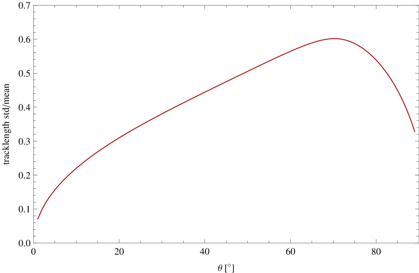
Figure 4: The relative standard deviation $\sqrt{{{\mathrm{Var}}\left\{{\raisebox{-1.72218pt}{\leavevmode\resizebox{}{6.02773pt}{$\mathcal{P}$}}_{L}(L\mid\theta)}\right\}}}/\bar{L}(\theta)$ of the tracklength as a function of the zenith angle $\theta$.

References

- [1] C. Pryke, “Geometrical design studies for water Cherenkov detectors via simulation,” Tech. Rep. GAP-96-008, Auger Project Technical Note, 1996.
- [2] FCEyN & Tandar Groups, “Simulations with GEANT,” Tech. Rep. GAP-96-011, Auger Project Technical Note, 1996.
- [3] C. Pryke, “Performance simulations of a 10 m2 water Cherenkov detector and comparison with experiment,” Tech. Rep. GAP-97-004, Auger Project Technical Note, 1997.
- [4] D. Ravignani et al., “Calculation of the number of photoelectrons with the water Cherenkov detector model,” Tech. Rep. GAP-97-024, Auger Project Technical Note, 1997.
- [5] C. Pryke, “Self calibration of the water Cherenkov tanks: Simulation,” Tech. Rep. GAP-97-026, Auger Project Technical Note, 1997.
- [6] C. Bonifazi, P. Bauleo, A. Ferrero, A. Filevich, and A. Reguera, “Response of a water Cherenkov detector to oblique and quasi-horizontal muons,” Tech. Rep. GAP-01-018, Auger Project Technical Note, 2001.
- [7] A. Chou, “Vertical equivalent muon study with the Fermilab tank,” Tech. Rep. GAP-02-045, Auger Project Technical Note, 2002.
- [8] W. Slater, A. Tripathi, and K. Arisaka, “A GEANT3 simulation of Pierre Auger Surface Detector response to muons,” Tech. Rep. GAP-02-063, Auger Project Technical Note, 2002.
- [9] A. Etchegoyen, “Track geometry and smearing of the bump calibration,” Tech. Rep. GAP-02-078, Auger Project Technical Note, 2002.
- [10] G. Fernandez, A. Tripathi, and K. Arisaka, “Simulation of the Pierre Auger surface detector response using GEANT4,” Tech. Rep. GAP-03-054, Auger Project Technical Note, 2003.
- [11] D. Supanitsky and X. Bertou, “Semi-analytical model of the three-fold charge spectrum in a water Cherenkov tank,” Tech. Rep. GAP-03-113, Auger Project Technical Note, 2003.
- [12] G. Fernandez, E. Zas, T. Ohnuki, A. Tripathi, D. Barnhill, J. Lee, and K. A. abnd W.E. Slater, “Surface detector response using lookup table based on GEANT4 simulation,” Tech. Rep. GAP-04-045, Auger Project Technical Note, 2004.
- [13] M. Aglietta, “A direct measurement of the photoelectron number per vertical muon in the Capisa SD detector,” Tech. Rep. GAP-05-010, Auger Project Technical Note, 2005.
- [14] D. Dornic, F. Arneodo, I. Lhenry-Yvon, X. Bertou, C. Bonifazi, P. Ghia, C. Grunfeld, and T. Suomijarvi, “Calibration analysis: Capisa data,” Tech. Rep. GAP-05-101, Auger Project Technical Note, 2005.
- [15] D. Dornic, Développement et caractérisation de photomultiplicateurs hémisphériques pour les expériences d’astroparticules d’étalonnage des détecteurs de surface et analyse des gerbes horizontales de l’Observatoire Pierre Auger. PhD thesis, Université Paris XI, 2006. pdf.
- [16] J. Alvarez-Muñiz, G. Rodríguez-Fernández, I. Valiño, and E. Zas, “Update on the method for tank signal response (SdSignalUSC code),” Tech. Rep. GAP-09-038, Auger Project Technical Note, 2009.
- [17] A. Castellina and G. Navarra, “Separating the electromagnetic and muonic components in the FADC traces of the Auger Surface Detectors,” Tech. Rep. GAP-06-065, Auger Project Technical Note, 2006.
- [18] X. Garrido, A. Cordier, S. Dagoret-Campagne, B. Kégl, D. Monnier-Ragaigne, and M. Urban, “Measurement of the number of muons in Auger tanks by the FADC jump counting method,” Tech. Rep. GAP-07-060, Auger Project Technical Note, 2007.
- [19] P. Diep, “Comments on muon counting in the FADC traces of the Auger surface detector,” Tech. Rep. GAP-08-136, Auger Project Technical Note, 2008.
- [20] X. Garrido, B. Kégl, A. Cordier, S. Dagoret-Campagne, D. Monnier-Ragaigne, and M. Urban, “Update and new results from the FADC jump counting method,” Tech. Rep. GAP-09-023, Auger Project Technical Note, 2009.
- [21] C. Robert and G. Casella, Monte Carlo Statistical Methods. New York: Springer-Verlag, 2004.
- [22] J. Alvarez-Muñiz, G. Rodríguez-Fernández, I. Valiño, and E. Zas, “An alternative method for tank signal response and calculation,” Tech. Rep. GAP-05-054, Auger Project Technical Note, 2005.