Future cosmological sensitivity for hot dark matter axions

Abstract

We study the potential of a future, large-volume photometric survey to constrain the axion mass $m_{a}$ in the hot dark matter limit. Future surveys such as Euclid will have significantly more constraining power than current observations for hot dark matter. Nonetheless, the lowest accessible axion masses are limited by the fact that axions lighter than $\sim 0.15$ eV decouple before the QCD epoch, assumed here to occur at a temperature $T_{\rm QCD}\sim 170$ MeV; this leaves an axion population of such low density that its late-time cosmological impact is negligible. For larger axion masses, $m_{a}\gtrsim 0.15$ eV, where axions remain in equilibrium until after the QCD phase transition, we find that a Euclid-like survey combined with Planck CMB data can detect $m_{a}$ at very high significance. Our conclusions are robust against assumptions about prior knowledge of the neutrino mass. Given that the proposed IAXO solar axion search is sensitive to $m_{a}\lesssim 0.2$ eV, the axion mass range probed by cosmology is nicely complementary.

1 Introduction

Interest in the low-energy frontier of particle physics has surged over the past few years, especially in the area of axions and axion-like particles (ALPs) [1, 2, 3, 4]. The ADMX microwave cavity experiment is getting ready for its final push towards covering a well-motivated range of axion masses at the sensitivity required to find these elusive particles if they were the dark matter in our galaxy [5, 6, 7, 8, 9]. New ideas to broaden the range of search masses are vigorously discussed [10, 11, 12, 13, 14, 15, 16, 17, 18, 19, 20]. In Korea, an entire Center of the Institute for Basic Science, the Center for Axion and Precision Physics (CAPP), has been dedicated to the search for axion dark matter and related topics in precision physics [21]. At DESY, first steps have been taken towards the largest ever photon-regeneration experiment to search for ALPs [22]. At CERN, the CAST experiment to search for solar axions has almost completed its original mission [24, 25, 26, 27, 23, 28], and has paved the way for proposing a much larger next-generation axion helioscope, the International Axion Observatory (IAXO) [29, 30]. In no small amount, our present study is motivated by the IAXO proposal.

Axion helioscopes such as CAST and IAXO take advantage of the two-photo axion interaction vertex both as a source of axions in the sun via the Primakoff effect and for the back-conversion of axions into X-rays in a dipole magnet oriented towards the sun. However, this back-conversion is not effective if the photon-axion mass difference is too large. Therefore, in the $(m_{a},g_{a\gamma})$-parameter plane, where $g_{a\gamma}$ is the two-photon axion coupling strength, it has been traditionally difficult to probe the “axion line” on which the QCD axion models—as opposed to generic axion-like particles (ALPs)—reside. CAST has recently succeeded in touching the axion line in a narrow $m_{a}$ range around 1 eV [23]; it is the purpose of the proposed IAXO to push to greater sensitivity and in this way explore realistic axion parameter space. In this connection, we note that, independently of model dependence of the relationship between $g_{a\gamma}$ and $m_{a}$, cosmological hot dark matter bounds can provide a guide as to the largest axion masses that are worth exploring with such an experiment.

Current observations of the cosmic microwave background (CMB) anisotropies and the large-scale matter distribution already impose severe constraints on the hot dark matter abundance; in the axion interpretation, this constraint corresponds to an axion mass limit of around 1 eV [31, 32, 33, 34, 35, 36]. In the future, large-volume surveys such as the Euclid mission [37] will have a significantly enhanced sensitivity to hot dark matter [39, 38]. The aim of the present work, therefore, is to examine just what such a survey will be able to do for axion physics.

To achieve this goal, we begin in section 2 with a brief review of axion cosmology. In section 3 we set up the cosmological framework and in particular discuss the used data sets and the cosmological model space. The actual numerical analysis for different assumptions about the hot dark matter contribution of neutrinos is provided in section 4. We summarise and discuss our findings in section 5.

2 Axion cosmology

2.1 Hot and cold axion populations

The primary parameter characterising invisible axion models is the axion decay constant $f_{a}$, or, equivalently, the energy scale at which the Peccei-Quinn symmetry is spontaneously broken. Mixing with the $\pi^{0}$-$\eta$-$\eta^{\prime}$ mesons at low energies induces a mass for the axion, given approximately by

$$m_{a}=\frac{z^{1/2}}{1+z}\,\frac{f_{\pi}}{f_{a}}\,m_{\pi}=\frac{0.58~{}{\rm eV}}{f_{a}/10^{7}~{}{\rm GeV}}\,,$$ (2.1)

where $z=m_{u}/m_{d}$ is the up/down quark mass ratio. The value of $z$ lies in the range 0.38–0.58 [40], which leads to an uncertainty in the relationship between $m_{a}$ and $f_{a}$ of less than $\pm 5$%. Therefore, we may equally use $m_{a}$ as a characteristic parameter.

Figure 1 shows the “Lee-Weinberg curve for axions”, pieced together from several different production mechanisms [41]. Non-thermal production by the re-alignment mechanism and possibly by the decay of cosmic strings (CS) and domain walls (DW) produces a nonrelativistic population that can account for the cosmic cold dark matter. The thick black line in figure 1 shows the present-day cold axion energy density and its nominal uncertainty, assuming the Peccei-Quinn symmetry is broken after inflation so that each causal patch at the QCD epoch has a unique initial misalignment angle $\Theta_{\rm i}$ when the axion field begins to oscillate. We follow reference [42] concerning the contribution from strings and domain-wall decay; other authors find a somewhat smaller contribution [41, 43].

If the Peccei-Quinn symmetry is broken before inflation such that $\Theta_{\rm i}$ is the same in the entire observable universe, the axion abundance depends on $\Theta_{\rm i}^{2}$ and in this sense is a random number [41]. Figure 1 shows some examples for the cosmic axion abundance in this scenario as thin black lines for the indicated $\Theta_{\rm i}$ values. Note also that because the axion field in this case is present and massless during inflation, the quantum fluctuations it picks up independently of the inflaton field can later show up as isocurvature fluctuations in the CMB anisotropies unless the energy scale of inflation is sufficiently small [44, 45, 46, 47]. This scenario would have been excluded if the tensor-to-scalar ratio $r$ had been as high as initially claimed by the BICEP2 team [48], because $r=0.2$ corresponds to an unacceptably high inflation energy scale of $\sim 10^{14}$ GeV [49, 50, 51]. However, with the results of the recent combined analysis of BICEP2, Keck Array and Planck data [52] being consistent with $r=0$, reports of its demise may have been a bit premature.

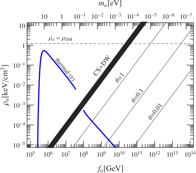
Figure 1: Present-day axion dark matter density as a function of $m_{a}$. The thermal axion population, which forms hot dark matter, is represented by the thick blue line. The thick black line denotes the cold axion population in the scenario in which Peccei-Quinn symmetry breaking occurs after inflation so that the visible universe contains many patches of different initial axion-field misalignment angles $\Theta_{\rm i}$; the energy density shown here subsumes both contributions from the re-alignment mechanism and from cosmic string (CS) and domain-wall (DW) decay according to reference [42]. The thin black lines pertain to the case in which Peccei-Quinn symmetry breaking occurs before inflation so that one single initial misalignment angle $\Theta_{\rm i}$ pervades the entire visible universe; the cold axion populations for several different values of $\Theta_{\rm i}$ as indicated at the lines are shown. (Figure adapted from one supplied by Javier Redondo.)

In addition, thermal processes produce axions which today play the role of hot dark matter [53]. The two populations co-exist because thermalisation of the cold population is extremely slow thanks to the axion derivative interactions with ordinary matter and photons, whose rates are suppressed at low energies. The thick blue line in figure 1 shows the hot dark matter density arising from thermal axion production. For axion masses $m_{a}\gtrsim 0.15$ eV, axion-pion interaction is the main production mechanism [54], and freeze-out occurs after the QCD epoch. However, as $m_{a}$ decreases and the freeze-out temperature approaches $T_{\rm QCD}\sim 170$ MeV, the freeze-out epoch suddenly jumps to a much higher temperature because axion interactions with gluons and quarks before confinement are much less efficient [55, 56, 57]. Furthermore, any thermal axion population frozen out before the QCD epoch is necessarily diluted by entropy production during the QCD epoch, which causes a sharp drop in the axion energy density in the transition region at $m_{a}\sim 0.15$ eV, as shown in figure 1. The exact transition between the pre- and post-QCD freeze-out regimes is not known, so we leave a gap in the blue curve. For very large axion masses, $m_{a}\gtrsim 20$ eV, the axion decay $a\to 2\gamma$ is fast relative to the age of the universe, so that the hot axion population disappears.

The contribution of thermally produced axions to the energy budget of the universe and hence the axion mass $m_{a}$ can be constrained by observations of CMB anisotropies and the large-scale structure distribution in the same way as we constrain neutrino hot dark matter and hence the neutrino mass sum. Our group has previously published limits on $m_{a}$ in a series of papers based on a sequence of cosmological data releases [31, 32, 33, 34, 35]; our most recent limit is $m_{a}\lesssim 0.67$ eV at 95% C.L. for a minimal cosmological model and using Planck-era cosmological data [35], a number comparable to the results of other authors [36]. Hot dark matter constraints do not apply to axion masses exceeding $\sim 20$ eV because the aforementioned $a\to 2\gamma$ decay removes the axion population. However, we note that axions masses up to $\sim 300$ keV are nonetheless cosmologically forbidden owing primarily to modifications to the primordial deuterium abundance instigated by the decay photons [58].

2.2 Axion decoupling temperature

The freeze-out history of the axion-pion interaction at temperatures below the QCD phase transition was studied in detail in reference [31]. This treatment is technically valid for $m_{a}\gtrsim 0.15$ eV and therefore adequate relative to the sensitivity of the present generation of cosmological probes because the current upper bound is $m_{a}\mbox{\;\raisebox{1.29167pt}{$<$}$\!\!\!\!\!$\raisebox{-3.87495pt}{$\sim$}\;}0.67$ eV [35]. However, an extension to lower axion masses would be useful in anticipation of the next generation of cosmological probes. This is especially so in view of the forecasted sensitivity of the Euclid mission to neutrino masses, $\sigma(m_{\nu})\sim 0.01$ eV [39]; considering the similar phenomenology, a decoupling model for axions down to similar masses should be contemplated.

Axions with very small masses decouple at temperatures above the QCD phase transition, where the axion interaction with free quarks and gluons can be studied perturbatively [56]. Perturbative treatments fail, however, when decoupling occurs close to the QCD epoch, and no full non-perturbative calculation exists to date. Therefore, to model axion decoupling in the mass range $0.01~{}{\rm eV}<m_{a}<1~{}{\rm eV}$, we use the following prescription.

1. We fix the QCD phase transition temperature $T_{\rm QCD}$ at a specific value. A typical choice might be $T_{\rm QCD}=170$ MeV, which conforms with the most recent calculations from lattice gauge theory [59, 60]. The chosen value of $T_{\rm QCD}$ does have an impact on the axion mass range that can be probed using large-scale structure observation, and we shall return to this point later.

2. For large axion masses ($m_{a}\gtrsim 0.2$ eV) we continue to use the same decoupling calculation as in previous works. We extend this calculation down to an axion mass at which it returns a decoupling temperature matching $T_{\rm QCD}$. For the choice of $T_{\rm QCD}=170$ MeV, this corresponds to $m_{a}=0.145$ eV. For all axion masses smaller than this limit, freeze-out occurs at $T>T_{\rm QCD}$.

3. For all axion masses smaller than this limiting value, we assume an effective number of entropy degrees of freedom of $g_{*}=80$ at the time of freeze-out, independently of the exact axion mass. This approximation is reasonable because $g_{*}(T)$ varies only logarithmically with temperature from $g_{*}\sim 60$ at $T_{\rm QCD}\sim 170$ MeV to $g_{*}\sim 100$ at the electroweak phase transition $T_{\rm EW}\sim 100$ GeV, in contrast with the step-like variation in the spate of a few MeVs during the QCD phase transition (see figure 3 of reference [61]).

As we shall see later, axions decoupling at temperatures above $T_{\rm QCD}$ are practically invisible to the surveys discussed here, whereas axions decoupling after the QCD epoch have a clear impact on cosmological observations.

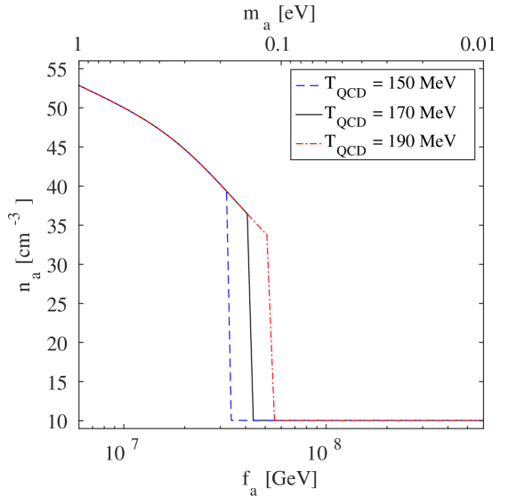
Figure 2: Present-day axion number density as a function of the axion mass (upper horizontal axis) and of the axion decay constant (lower horizontal axis), assuming $T_{\rm QCD}=170$ MeV (solid black line), $T_{\rm QCD}=150$ MeV (dashed blue line) and $T_{\rm QCD}=190$ MeV (dash-dotted red line).

Figure 2 shows the present-day axion number density as a function of the axion mass according to the model described above. For the choice of $T_{\rm QCD}=170$ MeV, the number density plummets from $n_{a}=36.45\,{\rm cm}^{-3}$ to $10.04\,{\rm cm}^{-3}$ at $m_{a}=0.145$ eV, reflecting the jump of the axion decoupling temperature when the universe transits through the QCD epoch. Since the dividing line hinges strongly on the assumed value of $T_{\rm QCD}$, we show also the cases of $T_{\rm QCD}=150$ and 190 MeV, where the corresponding drops in $n_{a}$ occur at $m_{a}=0.185$ and 0.117 eV, respectively. Given the uncertainty in $T_{\rm QCD}$ and the lack of a full quantitative calculation of the axion freeze-out in this temperature region, we cannot state the sensitivity to axion masses any more precisely. Henceforth, we shall use $T_{\rm QCD}=170$ MeV as our benchmark case, and

$$m_{\rm QCD}=0.145~{}{\rm eV}$$ (2.2)

shall denote the limiting axion mass corresponding to nominal freeze-out at this temperature.

3 Cosmological set-up

3.1 Cosmological mock data

In order to assess the sensitivity of future cosmological observations to the axion mass we use the parameter forecast code first described in reference [39] for galaxy clustering and cosmic shear surveys, and later extended in reference [38] to include cluster measurements. We adopt the same assumptions about the observational data, which conform to the specifications of the upcoming Euclid mission [37]. A summary of the mock data sets is as follows.

1. The cosmic shear auto-spectrum $C_{\ell,ij}^{\rm ss}$ runs in the range $2\leq\ell\leq\ell_{\rm max}^{\rm s}=2000$, and the indices $i,j\in[1,N_{\rm s}]$ label the redshift bin. As discussed in reference [39], shot-noise always dominates well before $\ell$ reaches $2000$, so that the precise value chosen for $\ell_{\rm max}$ is not critical. Redshift slicing is performed in such a way that all bins contain similar numbers of source galaxies and hence suffer the same amount of shot noise. We choose $N_{\rm s}=2$, as no substantial improvement in the parameter sensitivities can be expected beyond this point [39].

2. The galaxy auto-spectrum $C_{\ell,ij}^{\rm gg}$ uses multipole moments running from $\ell=2$ to $\ell^{{\rm g},i}_{\rm max}$ in redshift bins $i,j\in[1,N_{\rm g}]$, where $\ell^{{\rm g},i}_{\rm max}$ is set following the prescription of reference [39] so as to minimise the non-linear contamination. As shown in the said paper, most cosmological parameter sensitivities saturate at around $N_{\rm g}=11$; we shall also adopt this value. The linear galaxy bias is assumed to be perfectly known. While this assumption is not very realistic, in the absence of a concrete bias model the only alternative would be to adopt the opposite extreme in which the bias is completely unknown and uncorrelated between redshift bins. We have tested this equally unrealistic assumption in a previous work [39], and found that the resulting parameter constraints are utterly uncompetitive if the galaxy data were used on their own, and, if analysed in combination with shear data, hardly better than the shear-only constraints. We therefore do not consider the case of an unknown galaxy bias in the present work.

3. The shear–galaxy cross-spectrum $C_{\ell,ij}^{\rm sg}$ in the shear redshift bin $i\in[1,N_{\rm s}]$ and galaxy redshift bin $j\in[1,N_{\rm g}]$ runs from $\ell=2$ to $\ell^{{\rm g},j}_{\rm max}$, where $\ell^{{\rm g},j}_{\rm max}$ is determined by the galaxy redshift binning.

4. The cluster mass function measurements $N_{i,j(i)}$ source from clusters in the redshift range $z\in[0.01,z_{\rm high}]$ and with masses $M\in[M_{\rm thr}(z),10^{16}~{}M_{\odot}]$, where $M_{\rm thr}(z)$ is the redshift-dependent mass detection threshold, and $z_{\rm high}$ the redshift at which $M_{\rm thr}(z)$ exceeds $10^{16}~{}M_{\odot}$. The index $i\in[1,N_{z}]$ labels the redshift bins, with boundaries chosen such that for the fiducial model all bins contain equal numbers of clusters. In each redshift bin $i$ we further subdivide the cluster sample into mass bins $j(i)\in[1,N_{\mathrm{m}}]$, again demanding that the same number of clusters should fall into each bin [38].

5. A mock data set from a Planck-like CMB measurement is generated according to the procedure of reference [62], together with modifications according to reference [63] so that it better captures some of the gross features of the realistic Planck likelihood, such as the fact that its effective sky coverage is scale-dependent.

3.2 Cosmological model space

We use an 8-parameter cosmological model ${\bm{\Theta}}$, consisting of six “vanilla” parameters ${\bm{\Theta}}^{(6)}$, extended by the sum of neutrino masses here denoted as $m_{\nu}$ and the axion mass $m_{a}$, i.e.,

$${\bm{\Theta}}\equiv\Bigl{(}{\bm{\Theta}}^{(6)},m_{\nu},m_{a}\Bigr{)}\equiv\Bigl{(}(\omega_{\rm cdm},\omega_{\rm b},h,\ln(10^{10}A_{\rm s}),n_{\rm s}),m_{\nu},m_{a}\Bigr{)}.$$ (3.1)

Here, $\omega_{\rm cdm}\equiv\Omega_{\rm cdm}h^{2}$ and $\omega_{\rm b}\equiv\Omega_{\rm b}h^{2}$ are the present-day physical CDM and baryon densities respectively, $h\equiv H_{0}/(100{\rm~{}km/s/Mpc})$ is the dimensionless Hubble parameter, $\ln(10^{10}A_{\rm s})$ and $n_{\rm s}$ denote respectively the amplitude and spectral index of the initial scalar fluctuations, and $z_{\rm re}$ is the reionisation redshift.

For the part of the parameter space not related to neutrinos or axions, our fiducial model is defined by the parameter values

$${\bm{\Theta}}^{(6)}_{\rm fid}=\left(0.0226,0.1126587,0.7,2.1\times 10^{-9},0.96,11\right),$$ (3.2)

while for $m_{\nu}$ and $m_{a}$ we shall test a variety of fiducial values. Specifically, for the axion mass we use a range of values

$$m_{a{\rm,fid}}=0.01,0.1,0.15,0.2,0.5~{}{\rm eV},$$ (3.3)

covering the possibility of axion freeze-out both before and after the QCD phase transition (see figure 2). Neutrinos provide another source of hot dark matter of an unknown size. We expect their phenomenology to be similar to that of axions so that $m_{\nu}$ and $m_{a}$ are likely to be correlated. Therefore, we vary also the fiducial neutrino mass sum in the range

$$m_{\nu{\rm,fid}}=0.06,0.11,0.3,0.7,1~{}{\rm eV},$$ (3.4)

i.e., from the minimal mass allowed in the normal hierarchy by neutrino oscillation experiments, to well beyond the current cosmological upper bound.

Our analysis assumes, for the most part, a pessimistic scenario in which the neutrino mass sum is an unknown that has to be fitted simultaneously with the axion mass to the mock data, possibly leading to a degradation of the sensitivity to the latter. However, we shall consider also an optimistic case in which the neutrino mass is taken to be infinitely well measured by other means (e.g., by tritium $\beta$-decay experiments); in practice this means we hold the neutrino mass sum fixed at its fiducial value when fitting the mock data.

Lastly, we note that a number of recent cosmological analyses have found hints for a small hot dark matter contribution due to either a nonzero neutrino mass sum or axion mass [64, 35]. These results are largely a consequence of tension between different observations within the minimal $\Lambda$CDM interpretation—notably, the conflicting values of $\sigma_{8}$ and $\Omega_{m}$ reported by cluster catalogues and by Planck’s CMB temperature anisotropy measurements—which tends to settle on a nonzero hot dark matter component as a middle ground. However, the tension between these observations may just as well indicate an incomplete understanding of the systematics [65].

Another example was the apparent conflict between the primordial tensor amplitudes inferred from Planck’s CMB temperature anisotropies and from the BICEP2 $B$-polarisation measurement. In this case, an increase to the universe’s dark radiation content [66, 67] had been proposed as a solution. However, in the end the discrepancy was shown to be due to insufficient modelling of the galactic polarised dust emission [52].

While the study of such tensions in actual data is interesting, for the purpose of this forecast we prefer not to artificially insert tensions into our mock data; we shall rather work with unbiased simulated observables, assuming that systematic issues in the measurements themselves will have been sorted out by the time the Euclid mission produces results.

4 Numerical results

4.1 Unknown neutrino mass

all
	$m_{\nu{\rm,fid}}=0.06~{}{\rm eV}$	$m_{\nu{\rm,fid}}=0.11~{}{\rm eV}$	$m_{\nu{\rm,fid}}=0.3~{}{\rm eV}$	$m_{\nu{\rm,fid}}=0.7~{}{\rm eV}$	$m_{\nu{\rm,fid}}=1~{}{\rm eV}$
$m_{a{\rm,fid}}=0.01~{}{\rm eV}$	$0\,-\,0.136$	$0\,-\,0.136$	$0\,-\,0.144$	$0\,-\,0.137$	$0\,-\,0.144$
$m_{a{\rm,fid}}=0.1~{}{\rm eV}$	$0\,-\,0.144$	$0\,-\,0.144$	$0\,-\,0.144$	$0\,-\,0.137$	$0\,-\,0.144$
$m_{a{\rm,fid}}=0.15~{}{\rm eV}$	$0.145\,-\,0.256$	$0.145\,-\,0.281$	$0.145\,-\,0.286$	$0.145\,-\,0.303$	$0.145\,-\,0.317$
$m_{a{\rm,fid}}=0.2~{}{\rm eV}$	$0.155\,-\,0.302$	$0.155\,-\,0.318$	$0.158\,-\,0.352$	$0.154\,-\,0.331$	$0.155\,-\,0.359$
$m_{a{\rm,fid}}=0.5~{}{\rm eV}$	$0.415\,-\,0.570$	$0.400\,-\,0.567$	$0.383\,-\,0.566$	$0.392\,-\,0.569$	$0.341\,-\,0.581$
ccl
	$m_{\nu{\rm,fid}}=0.06~{}{\rm eV}$	$m_{\nu{\rm,fid}}=0.11~{}{\rm eV}$	$m_{\nu{\rm,fid}}=0.3~{}{\rm eV}$	$m_{\nu{\rm,fid}}=0.7~{}{\rm eV}$	$m_{\nu{\rm,fid}}=1~{}{\rm eV}$
$m_{a{\rm,fid}}=0.01~{}{\rm eV}$	$0\,-\,0.144$	$0\,-\,0.144$	$0\,-\,0.144$	$0\,-\,0.135$	$0\,-\,0.144$
$m_{a{\rm,fid}}=0.1~{}{\rm eV}$	$0\,-\,0.136$	$0\,-\,0.138$	$0\,-\,0.137$	$0\,-\,0.137$	$0\,-\,0.137$
$m_{a{\rm,fid}}=0.15~{}{\rm eV}$	$0.145\,-\,0.392$	$0.145\,-\,0.507$	$0.145\,-\,0.749$	$0.145\,-\,0.706$	$0.145\,-\,0.893$
$m_{a{\rm,fid}}=0.2~{}{\rm eV}$	$0.157\,-\,0.407$	$0.161\,-\,0.531$	$0.168\,-\,0.825$	$0.169\,-\,0.869$	$0.173\,-\,0.902$
$m_{a{\rm,fid}}=0.5~{}{\rm eV}$	$0.233\,-\,0.642$	$0.204\,-\,0.765$	$0.266\,-\,0.933$	$0.226\,-\,1.033$	$0.253\,-\,1.107$
csgx
	$m_{\nu{\rm,fid}}=0.06~{}{\rm eV}$	$m_{\nu{\rm,fid}}=0.11~{}{\rm eV}$	$m_{\nu{\rm,fid}}=0.3~{}{\rm eV}$	$m_{\nu{\rm,fid}}=0.7~{}{\rm eV}$	$m_{\nu{\rm,fid}}=1~{}{\rm eV}$
$m_{a{\rm,fid}}=0.01~{}{\rm eV}$	$0\,-\,0.137$	$0\,-\,0.137$	$0\,-\,0.144$	$0\,-\,0.136$	$0\,-\,0.137$
$m_{a{\rm,fid}}=0.1~{}{\rm eV}$	$0\,-\,0.144$	$0\,-\,0.136$	$0\,-\,0.144$	$0\,-\,0.137$	$0\,-\,0.137$
$m_{a{\rm,fid}}=0.15~{}{\rm eV}$	$0.145\,-\,0.309$	$0.145\,-\,0.309$	$0.145\,-\,0.355$	$0.145\,-\,0.331$	$0.145\,-\,0.354$
$m_{a{\rm,fid}}=0.2~{}{\rm eV}$	$0.151\,-\,0.311$	$0.155\,-\,0.330$	$0.153\,-\,0.387$	$0.154\,-\,0.352036$	$0.157\,-\,0.381$
$m_{a{\rm,fid}}=0.5~{}{\rm eV}$	$0.412\,-\,0.570$	$0.396\,-\,0.567$	$0.361\,-\,0.566$	$0.375\,-\,0.563$	$0.278\,-\,0.584$
cs
	$m_{\nu{\rm,fid}}=0.06~{}{\rm eV}$	$m_{\nu{\rm,fid}}=0.11~{}{\rm eV}$	$m_{\nu{\rm,fid}}=0.3~{}{\rm eV}$	$m_{\nu{\rm,fid}}=0.7~{}{\rm eV}$	$m_{\nu{\rm,fid}}=1~{}{\rm eV}$
$m_{a{\rm,fid}}=0.01~{}{\rm eV}$	$0\,-\,0.137$	$0\,-\,0.137$	$0\,-\,0.144$	$0\,-\,0.144$	$0\,-\,0.144$
$m_{a{\rm,fid}}=0.1~{}{\rm eV}$	$0\,-\,0.144$	$0\,-\,0.137$	$0\,-\,0.144$	$0\,-\,0.137$	$0\,-\,0.144$
$m_{a{\rm,fid}}=0.15~{}{\rm eV}$	$0.145\,-\,0.321$	$0.145\,-\,0.350$	$0.145\,-\,0.513$	$0.145\,-\,0.704$	$0.145\,-\,0.824$
$m_{a{\rm,fid}}=0.2~{}{\rm eV}$	$0.152\,-\,0.349$	$0.157\,-\,0.374$	$0.161\,-\,0.528$	$0.164\,-\,0.738$	$0.166\,-\,0.838$
$m_{a{\rm,fid}}=0.5~{}{\rm eV}$	$0.200\,-\,0.585$	$0.186\,-\,0.604$	$0.208\,-\,0.711$	$0.187\,-\,0.865$	$0.218\,-\,0.941$

Table 1: 1D marginal 95% credible intervals for the axion mass inferred from four different data combinations (indicated above the panels; see text for an explanation of the abbreviations), assuming different fiducial $m_{a}$ and $m_{\nu}$ values.

Table 1 shows the allowed ranges of axion masses for our 25 different combinations of fiducial axion and neutrino mass values, inferred from four combinations of data set:

• ccl: CMB + clusters,

• cs: CMB + shear auto-spectrum,

• csgx: CMB + shear auto-correlation + galaxy auto-correlation + shear-galaxy cross-correlation, and

• all: CMB + shear auto-correlation + galaxy auto-correlation + shear-galaxy cross correlation + clusters.

The “jump effect” discussed in section 2.2 is immediately apparent: for fiducial axion masses below $m_{\rm QCD}=0.145$ eV, it is not possible to diagnose a nonzero axion mass even with a future mission such as Euclid. This is in sharp contrast to the case of neutrino masses, where it has been shown that even the minimum mass sum of $m_{\nu}=0.06$ eV can be detected by Euclid with high statistical significance [39]. As explained earlier, this is because axions with masses smaller than $m_{\rm QCD}$ decouple at temperatures above $T_{\rm QCD}=170$ MeV, so that their corresponding present-day number densities suffer from entropy dilution acquired during the QCD phase transition, as already illustrated in figure 2; in contrast, the present-day neutrino number density is always $n_{\nu}=112~{}{\rm cm}^{-3}$ per flavour, independently of the neutrino mass. As soon as the fiducial axion mass exceeds $m_{\rm QCD}$, however, a positive detection becomes easily possible.

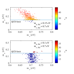
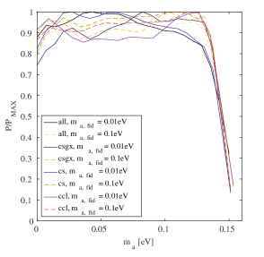
Figure 3: Left: Scatter plot of inferred mass values in the $m_{a}$-$m_{\nu}$ plane, assuming a common $m_{\nu{\rm,fid}}=0.7$ eV, and $m_{a{\rm,fid}}=0.15\ {\rm eV}>m_{\rm QCD}$ (top) and $m_{a{\rm,fid}}=0.10\ {\rm eV}<m_{\rm QCD}$ (bottom). The combination of all data sets is considered in both cases. The colours of the points indicate the corresponding axion number density according to the colour bar. Right: 1D marginal posterior probability density distribution in $m_{a}$ inferred from various combinations of data sets, assuming $m_{\nu{\rm,fid}}=0.06\,{\rm eV}$ and two choices of fiducial axion masses below the QCD mass limit.

We further illustrate this jump effect in the left panel of figure 3, which shows two scatter plots of the $m_{a}$ and $m_{\nu}$ values from the likelihood analysis of the “all” data combination, assuming a common $m_{\nu{\rm,fid}}=0.7$ eV but two different $m_{a,{\rm fid}}$ values: one just above $m_{\rm QCD}$ in the top panel ($m_{a,{\rm fid}}=0.15$ eV), and one just below in the bottom ($m_{a,{\rm fid}}=0.1$ eV). The axion number density corresponding to each scatter point is denoted by its colour coding. Clearly, in the top panel, the likelihood analysis returns a high concentration of points at the fiducial axion mass value. In the usual fashion the rest of the points are scattered around $m_{a,{\rm fid}}$, but with the twist that the density of points is sharply reduced for axion masses below $m_{\rm QCD}$, the QCD phase transition mass limit.

A similar cut-off can also be seen in the bottom panel, except that in this case, because $m_{a,{\rm fid}}<m_{\rm QCD}$, it is those axion masses exceeding $m_{\rm QCD}$ that are devoid of scatter points, all of which are now spread instead between $0$ eV and $m_{\rm QCD}$. Indeed, the probability distribution between $m_{a}=0$ eV and $m_{\rm QCD}$ is essentially flat in the $m_{a}$-direction no matter the exact choice of $m_{a,{\rm fid}}$, as demonstrated in the right panel of figure 3 by the 1D marginal posteriors for a selection of $m_{a,{\rm fid}}$ values. This flatness signifies that the $m_{a,{\rm fid}}<m_{\rm QCD}$ cases are for all purposes indistinguishable from one another.

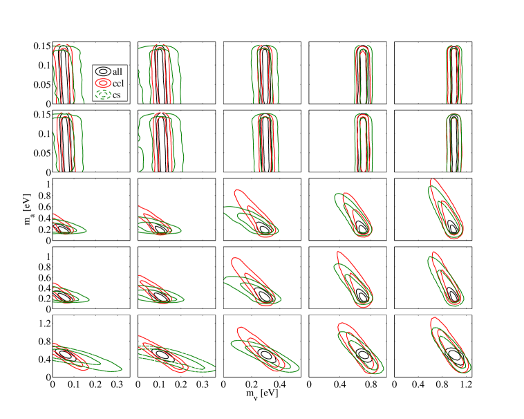
Figure 4: 2D marginal 68% and 95% credible contours for $m_{a}$ and $m_{\nu}$ derived from the “ccl” (red), “cs” (green), and “all” (black) data combinations. The matrix of fiducial mass combinations is the same as in table 1.

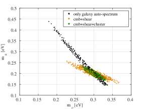
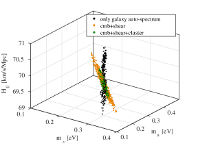
Figure 5: Scatter plot in the 3D $(H_{0},m_{a},m_{\nu})$-parameter space for the fiducial mass combination $m_{a,{\rm fid}}=0.2$ eV and $m_{\nu,{\rm fid}}=0.3$ eV. The orange points denote the “cs” data combination, the green points “cs+clusters”, and the black points the galaxy auto-spectrum. The MCMC fitting has been performed only in this 3D subspace, while all other parameters have been held fixed at their fiducial values. For improved readability we plot only those points satisfying $\Delta\chi^{2}\leq 2$.

Lastly, figure 4 shows the 68% and 95% contours in the 2D $(m_{a},m_{\nu})$-parameter space derived from various data combinations and for the full matrix of fiducial mass values shown in table 1. For most fiducial mass combinations there is a strong degeneracy between $m_{\nu}$ and $m_{a}$ when the “ccl” and “cs” data combinations are considered separately. This degeneracy is however almost entirely broken for the “all” data combination, where the galaxy auto-spectrum is also fitted along with shear and cluster data. To understand why this happens, consider the scatter plot in the 3D $(H_{0},m_{a},m_{\nu})$-parameter space displayed in figure 5. Evidently, the degeneracy directions resulting from the “cs” and “cs+clusters” data combinations are close to orthogonal to that from the galaxy auto-spectrum alone. Thus, adding the galaxy auto-spectrum not only breaks the degeneracy between $m_{a}$ and $m_{\nu}$, but also the two parameters’ respective degeneracies with $H_{0}$.

4.2 Fixed neutrino mass

Cosmological data of the accuracy studied here will not be available until about a decade from now. It is therefore conceivable that the neutrino mass will have been pinned down before then, via, e.g., measurements of tritium decay by the KATRIN experiment or by a post-KATRIN generation experiment [68]. We therefore study also the extreme case in which the neutrino mass is assumed to be exactly known, in order to assess the maximum possible effect our prior knowledge of neutrino masses has on the cosmological sensitivity to axion masses. We consider the same 25 combinations of fiducial axion and neutrino masses, but vary now only the axion mass as a fit parameter. The likelihood analysis is restricted to the “all” combination of data sets.

Table 2 shows the allowed $m_{a}$ ranges for all 25 combinations of $m_{a,{\rm fid}}$ and $m_{\nu,{\rm fid}}$. Comparing with their counterparts in table 1, we can immediately make the following observations: On the one hand, for fiducial axion masses below the QCD mass limit, what happens to the neutrino mass continues to have virtually no impact on the sensitivity to $m_{a}$. On the other hand, in those cases where $m_{a,{\rm fid}}$ exceeds $m_{\rm QCD}$, the corresponding error bands shrink by $\sim 30\%$ to $\sim 60\%$ upon fixing the neutrino mass.

all, fixed neutrino masses
	$m_{\nu{\rm,fid}}=0.06~{}{\rm eV}$	$m_{\nu{\rm,fid}}=0.11~{}{\rm eV}$	$m_{\nu{\rm,fid}}=0.3~{}{\rm eV}$	$m_{\nu{\rm,fid}}=0.7~{}{\rm eV}$	$m_{\nu{\rm,fid}}=1~{}{\rm eV}$
$m_{a{\rm,fid}}=0.01~{}{\rm eV}$	$0\,-\,0.135$	$0\,-\,0.134$	$0\,-\,0.136$	$0\,-\,0.137$	$0\,-\,0.137$
$m_{a{\rm,fid}}=0.1~{}{\rm eV}$	$0\,-\,0.138$	$0\,-\,0.137$	$0\,-\,0.137$	$0\,-\,0.144$	$0\,-\,0.137$
$m_{a{\rm,fid}}=0.15~{}{\rm eV}$	$0.140\,-\,0.211$	$0.140\,-\,0.213$	$0.140\,-\,0.212$	$0.140\,-\,0.215$	$0.140\,-\,0.223$
$m_{a{\rm,fid}}=0.2~{}{\rm eV}$	$0.159\,-\,0.250$	$0.158\,-\,0.253$	$0.157\,-\,0.253$	$0.157\,-\,0.256$	$0.154\,-\,0.256$
$m_{a{\rm,fid}}=0.5~{}{\rm eV}$	$0.454\,-\,0.544$	$0.453\,-\,0.545$	$0.454\,-\,0.544$	$0.455\,-\,0.543$	$0.454\,-\,0.543$

Table 2: 1D marginal 95% credible intervals for the axion mass inferred from the “all” data combination, assuming different fiducial $m_{a}$ and $m_{\nu}$ values. In each case the neutrino mass has been fixed at the fiducial value in the analysis.

These results can be understood from an inspection of the 2D marginal credible contours in figure 4. When the neutrino mass is left as a free parameter, construction of the 1D marginal posterior for the axion mass $m_{a}$ consists essentially of integrating the 2D ellipse along the $m_{\nu}$-direction. With the neutrino mass fixed, however, the 1D marginal posterior for $m_{a}$ is simply the cross-section of the ellipse at $m_{\nu}=m_{\nu,{\rm fid}}$. Thus, because the ellipses in the $m_{a,{\rm fid}}<m_{\rm QCD}$ cases are almost exactly aligned with the $m_{a}$-axis, the two procedures yield very similar results. In contrast, the ellipses in the $m_{a,{\rm fid}}>m_{\rm QCD}$ scenarios are all inclined at an angle; assuming that the ellipses represent perfect 2D Gaussian distributions, integration along the $m_{\nu}$-direction will always yield a 1D posterior for $m_{a}$ that is broader than the cross-section at $m_{\nu}=m_{\nu,{\rm fid}}$, with the greatest disparity occurring when the inclination approaches $45^{\circ}$.

4.3 When can a detection be claimed?

Having calculated the formal sensitivity to $m_{a}$ for a variety of different fiducial models we might now also ask the question: How strongly would a model with $m_{a}=0$ be disfavoured depending on the assumed fiducial model?

Table 3 shows the $\Delta\chi^{2}$ values for the best-fit model assuming $m_{a}=0$, relative to the global best fit (i.e., the fiducial model), derived from the “all” data set for the 25 fiducial mass combinations. (Note that we have also varied the neutrino mass as a fit parameter.) Looking at the first two rows, it is immediately clear that fiducial axion masses below 0.15 eV, for which $\Delta\chi^{2}\simeq 0$, will not in practice be distinguishable from zero given the accuracy of the data used here. This conclusion is consistent with our understanding of the Bayesian results presented in section 4.1 and 4.2.

As soon as the fiducial axion mass surpasses 0.15 eV, the $\Delta\chi^{2}$ value jumps to the range 13–37, depending on the fiducial neutrino mass; the larger the $m_{\nu,{\rm fid}}$ value, the lower the $\Delta\chi$. Physically, this trend can be traced to a very small residual degeneracy between $m_{a}$ and $m_{\nu}$, so that a 1 eV neutrino could partially fill in the role of a 0.15 eV axion while a 0.06 eV neutrino could not. But this is ultimately only an academic point of interest, because $\Delta\chi^{2}$ values as large as 13–37 at the cost of just one additional fit parameter would in any case constitute “strong” evidence in favour of a nonzero axion mass, no matter whether we apply the Bayes information criterion (BIC), the Akaike information criterion (AIC), or other constructs.

We therefore conclude that for any axion mass above the mass threshold $0.15$ eV required for the axion to decouple after the QCD epoch, Planck data in combination with a Euclid-like photometric survey will have sufficient accuracy to reliably measure the axion mass. If on the other hand the real axion mass falls below the QCD mass threshold, then the corresponding axion number density is so low that a future survey with a much better accuracy would be needed to further tighten the axion mass bound from above.

	$m_{\nu{\rm,fid}}=0.06~{}{\rm eV}$	$m_{\nu{\rm,fid}}=0.11~{}{\rm eV}$	$m_{\nu{\rm,fid}}=0.3~{}{\rm eV}$	$m_{\nu{\rm,fid}}=0.7~{}{\rm eV}$	$m_{\nu{\rm,fid}}=1~{}{\rm eV}$
$m_{a{\rm,fid}}=0.01~{}{\rm eV}$	$0$	$0$	$0$	$0$	$0$
$m_{a{\rm,fid}}=0.1~{}{\rm eV}$	$0$	$0$	$0$	$0$	$0$
$m_{a{\rm,fid}}=0.15~{}{\rm eV}$	$37$	$36$	$31$	$18$	$13$
$m_{a{\rm,fid}}=0.2~{}{\rm eV}$	$47$	$46$	$40$	$25$	$18$
$m_{a{\rm,fid}}=0.5~{}{\rm eV}$	$75$	$71$	$64$	$55$	$38$

Table 3: $\Delta\chi^{2}$ values (rounded to the nearest whole number) for the best-fit model assuming $m_{a}$ fixed at zero, relative to the global best-fit, derived from the “all” data set for the 25 fiducial mass combinations.

5 Conclusions

The next generation of large-volume photometric surveys, notably Euclid, together with CMB data from the Planck mission are almost guaranteed to reach a sensitivity to the cosmic hot dark matter content good enough to measure the sum of neutrino masses $\sum m_{\nu}$ with high significance. This is so even if $\sum m_{\nu}$ should take on its most pessimistic value, 60 meV, the minimum established by flavour oscillation experiments. Complementarily, laboratory experiments will provide a direct measurement of the effective electron neutrino mass, albeit likely on a longer timescale. Depending on what is actually found at these experiments, there will be a new frontier of either identifying an additional hot dark matter component, or placing very precise constraints on non-neutrino contributions, e.g., in the form of a hot axion population.

Motivated by the IAXO proposal for a next-generation solar axion search, we have explored the range of axion masses that is accessible to cosmological hot dark matter searches. For large enough axion masses, thermal axions are produced after the QCD epoch by very efficient axion-pion interactions, so that the resulting axion population is almost comparable to that of one species of neutrinos. For small masses, however, axion freeze-out occurs before the QCD epoch, where axion production from interactions with free quarks and gluons is much less efficient, and the final axion population is invariably diluted by the large number of colour degrees of freedom that disappear when the temperature of the universe drops below $T_{\rm QCD}$.

Based on this understanding, and assuming that $T_{\rm QCD}=170$ MeV, we find that axion masses larger than $\sim 0.15$ eV can be easily pinned down by cosmology. If on the other hand the axion mass is lower than this threshold, then cosmological observations are essentially blind to the hot axion population for the foreseeable future.

When optimising the IAXO apparatus and search strategies, we conclude that the mass range $m_{a}\lesssim 0.15~{}{\rm eV}$ should have the highest priority because larger axion masses can be constrained by cosmology. To study this higher mass range with IAXO requires helium filling of the conversion region to achieve a match between the axion search mass and the refractive photon mass, a method that has been used at CAST and requires sequential pressure settings to cover a broad range of axion search masses. Therefore, cosmology can help to simplify the IAXO search strategy in that the technically most difficult mass range may well have been excluded by cosmology before IAXO becomes operational.

References

- [1] J. Jaeckel and A. Ringwald, “The low-energy frontier of particle physics,” Ann. Rev. Nucl. Part. Sci. 60 (2010) 405 [arXiv:1002.0329].
- [2] J. L. Hewett et al., “Fundamental physics at the intensity frontier,” arXiv:1205.2671.
- [3] R. Essig et al., “Dark sectors and new, light, weakly-coupled particles,” arXiv:1311.0029.
- [4] K. Baker et al., “The quest for axions and other new light particles,” Annalen Phys. 525 (2013) A93 [arXiv:1306.2841].
- [5] S. J. Asztalos et al. (ADMX Collaboration), “A SQUID-based microwave cavity search for dark-matter axions,” Phys. Rev. Lett. 104 (2010) 041301 [arXiv:0910.5914].
- [6] S. J. Asztalos et al. (ADMX Collaboration), “Design and performance of the ADMX SQUID-based microwave receiver,” Nucl. Instrum. Meth. A 656 (2011) 39 [arXiv:1105.4203].
- [7] K. van Bibber and G. Carosi, “Status of the ADMX and ADMX-HF experiments,” arXiv:1304.7803.
- [8] G. Rybka, “Direct detection searches for axion dark matter,” Phys. Dark Univ. 4 (2014) 14.
- [9] A. Cho, “Dark matter’s dark horse,” Science 342 (2013) 552.
- [10] O. K. Baker et al., “Prospects for searching axion-like particle dark matter with dipole, toroidal and wiggler magnets,” Phys. Rev. D 85, 035018 (2012) [arXiv:1110.2180].
- [11] D. Horns, J. Jaeckel, A. Lindner, A. Lobanov, J. Redondo and A. Ringwald, “Searching for WISPy cold dark matter with a dish antenna,” JCAP 1304 (2013) 016 [arXiv:1212.2970].
- [12] J. Jaeckel and J. Redondo, “An antenna for directional detection of WISPy dark matter,” JCAP 1311 (2013) 016 [arXiv:1307.7181].
- [13] J. Jaeckel and J. Redondo, “From resonant to broadband searches for WISPy cold dark matter,” Phys. Rev. D 88 (2013) 115002 [arXiv:1308.1103].
- [14] D. Horns, A. Lindner, A. Lobanov and A. Ringwald, “WISPers from the dark side: Radio probes of axions and hidden photons,” arXiv:1309.4170.
- [15] P. Sikivie, N. Sullivan and D. B. Tanner, “Axion dark matter detection using an LC circuit,” arXiv:1310.8545.
- [16] G. Rybka and A. Wagner, “A technique to search for high mass dark matter axions,” arXiv:1403.3121.
- [17] P. W. Graham and S. Rajendran, “Axion dark matter detection with cold molecules,” Phys. Rev. D 84 (2011) 055013 [arXiv:1101.2691].
- [18] P. W. Graham and S. Rajendran, “New observables for direct detection of axion dark matter,” Phys. Rev. D 88 (2013) 035023 [arXiv:1306.6088].
- [19] D. Budker, P. W. Graham, M. Ledbetter, S. Rajendran and A. Sushkov, “Cosmic axion spin precession experiment (CASPEr),” Phys. Rev. X 4 (2014) 021030 [arXiv:1306.6089].
- [20] C. Beck, “Possible resonance effect of axionic dark matter in Josephson junctions,” Phys. Rev. Lett. 111 (2013) 231801 [arXiv:1309.3790].
- [21] Center for Axion and Precision Physics Research (CAPP), see http://capp.ibs.re.kr/html/capp_en/
- [22] R. Bähre et al., “Any light particle search II —Technical Design Report,” JINST 8 (2013) T09001
- [23] M. Arik et al. [CAST Collaboration], Phys. Rev. Lett. 112, no. 9, 091302 (2014) [arXiv:1307.1985 [hep-ex]]. [arXiv:1302.5647]. See also http://alps.desy.de/
- [24] K. Zioutas et al. (CAST Collaboration), “First results from the CERN Axion Solar Telescope (CAST),” Phys. Rev. Lett. 94 (2005) 121301 [hep-ex/0411033].
- [25] S. Andriamonje et al. (CAST Collaboration), “An improved limit on the axion-photon coupling from the CAST experiment,” JCAP 0704 (2007) 010 [hep-ex/0702006].
- [26] E. Arik et al. (CAST Collaboration), “Probing eV-scale axions with CAST,” JCAP 0902 (2009) 008 [arXiv:0810.4482].
- [27] S. Aune et al. (CAST Collaboration), “CAST search for sub-eV mass solar axions with 3He buffer gas,” Phys. Rev. Lett. 107 (2011) 261302 [arXiv:1106.3919].
- [28] K. Barth et al. (CAST Collaboration), “CAST constraints on the axion-electron coupling,” JCAP 1305 (2013) 010 [arXiv:1302.6283].
- [29] I. G. Irastorza et al., “Towards a new generation axion helioscope,” JCAP 1106 (2011) 013 [arXiv:1103.5334].
- [30] E. Armengaud et al., “Conceptual design of the International Axion Observatory (IAXO),” JINST 9 (2014) T05002 [arXiv:1401.3233].
- [31] S. Hannestad, A. Mirizzi and G. Raffelt, “New cosmological mass limit on thermal relic axions,” JCAP 0507 (2005) 002 [hep-ph/0504059].
- [32] S. Hannestad, A. Mirizzi, G. G. Raffelt and Y. Y. Y. Wong, “Cosmological constraints on neutrino plus axion hot dark matter,” JCAP 0708 (2007) 015 [arXiv:0706.4198].
- [33] S. Hannestad, A. Mirizzi, G. G. Raffelt and Y. Y. Y. Wong, “Cosmological constraints on neutrino plus axion hot dark matter: Update after WMAP-5,” JCAP 0804 (2008) 019 [arXiv:0803.1585].
- [34] S. Hannestad, A. Mirizzi, G. G. Raffelt and Y. Y. Y. Wong, “Neutrino and axion hot dark matter bounds after WMAP-7,” JCAP 1008 (2010) 001 [arXiv:1004.0695].
- [35] M. Archidiacono, S. Hannestad, A. Mirizzi, G. Raffelt and Y. Y. Y. Wong, “Axion hot dark matter bounds after Planck,” JCAP 1310 (2013) 020 [arXiv:1307.0615].
- [36] A. Melchiorri, O. Mena and A. Slosar, “An improved cosmological bound on the thermal axion mass,” Phys. Rev. D 76 (2007) 041303 [arXiv:0705.2695].
- [37] R. Laureijs et al. (EUCLID Collaboration), “Euclid Definition Study Report,” arXiv:1110.3193.
- [38] T. Basse, O. E. Bjaelde, J. Hamann, S. Hannestad and Y. Y. Y. Wong, “Dark energy properties from large future galaxy surveys,” JCAP 1405 (2014) 021 [arXiv:1304.2321].
- [39] J. Hamann, S. Hannestad and Y. Y. Y. Wong, “Measuring neutrino masses with a future galaxy survey,” JCAP 1211 (2012) 052 [arXiv:1209.1043].
- [40] A. V. Manohar and C. T. Sachrajda, “Quark masses,” in: K. A. Olive et al. (Particle Data Group), “Review of Particle Physics,” Chin. Phys. C 38 (2014) 090001.
- [41] P. Sikivie, “Axion cosmology,” Lect. Notes Phys. 741 (2008) 19 [astro-ph/0610440].
- [42] T. Hiramatsu, M. Kawasaki, K. Saikawa and T. Sekiguchi, “Production of dark matter axions from collapse of string-wall systems,” Phys. Rev. D 85 (2012) 105020; Erratum -ibid. 86 (2012) 089902 [arXiv:1202.5851].
- [43] L. Visinelli and P. Gondolo, “Dark matter axions revisited,” Phys. Rev. D 80 (2009) 035024 [arXiv:0903.4377].
- [44] D. H. Lyth, “A limit on the inflationary energy density from axion isocurvature fluctuations,” Phys. Lett. B 236 (1990) 408.
- [45] M. Beltrán, J. García-Bellido and J. Lesgourgues, “Isocurvature bounds on axions revisited,” Phys. Rev. D 75 (2007) 103507 [hep-ph/0606107].
- [46] M. P. Hertzberg, M. Tegmark and F. Wilczek, “Axion cosmology and the energy scale of inflation,” Phys. Rev. D 78 (2008) 083507 [arXiv:0807.1726].
- [47] J. Hamann, S. Hannestad, G. G. Raffelt and Y. Y. Y. Wong, “Isocurvature forecast in the anthropic axion window,” JCAP 0906 (2009) 022 [arXiv:0904.0647].
- [48] P. A. R. Ade et al. (BICEP2 Collaboration), “Detection of B-mode polarization at degree angular scales by BICEP2,” Phys. Rev. Lett. 112 (2014) 241101 [arXiv:1403.3985].
- [49] T. Higaki, K. S. Jeong and F. Takahashi, “Solving the tension between high-scale inflation and axion isocurvature perturbations,” Phys. Lett. B 734 (2014) 21 [arXiv:1403.4186].
- [50] D. J. E. Marsh, D. Grin, R. Hlozek and P. G. Ferreira, “Tensor detection severely constrains axion dark matter,” Phys. Rev. Lett. 113 (2014) 011801 [arXiv:1403.4216].
- [51] L. Visinelli and P. Gondolo, “Axion cold dark matter in view of BICEP2 results,” Phys. Rev. Lett. 113 (2014) 011802 [arXiv:1403.4594].
- [52] P. A. R. Ade et al. [BICEP2 and Planck Collaborations], [arXiv:1502.00612 [astro-ph.CO]].
- [53] M. S. Turner, “Thermal production of not so invisible axions in the early universe,” Phys. Rev. Lett. 59 (1987) 2489; Erratum ibid. 60 (1988) 1101.
- [54] S. Chang and K. Choi, “Hadronic axion window and the big bang nucleosynthesis,” Phys. Lett. B 316 (1993) 51 [hep-ph/9306216].
- [55] E. Massó, F. Rota and G. Zsembinszki, “On axion thermalization in the early universe,” Phys. Rev. D 66 (2002) 023004 [hep-ph/0203221].
- [56] P. Graf and F. D. Steffen, “Thermal axion production in the primordial quark-gluon plasma,” Phys. Rev. D 83 (2011) 075011 [arXiv:1008.4528].
- [57] A. Salvio, A. Strumia and W. Xue, “Thermal axion production,” JCAP 1401 (2014) 011 [arXiv:1310.6982].
- [58] D. Cadamuro, S. Hannestad, G. Raffelt and J. Redondo, “Cosmological bounds on sub-MeV mass axions,” JCAP 1102 (2011) 003 [arXiv:1011.3694].
- [59] A. Bazavov et al., “Equation of state and QCD transition at finite temperature,” Phys. Rev. D 80 (2009) 014504 [arXiv:0903.4379].
- [60] G. Endrodi, Z. Fodor, S. D. Katz and K. K. Szabo, “The QCD phase diagram at nonzero quark density,” JHEP 1104 (2011) 001 [arXiv:1102.1356].
- [61] C. Brust, D. E. Kaplan and M. T. Walters, “New light species and the CMB,” JHEP 1312 (2013) 058 [arXiv:1303.5379].
- [62] L. Perotto, J. Lesgourgues, S. Hannestad, H. Tu and Y. Y. Y. Wong, “Probing cosmological parameters with the CMB: Forecasts from full Monte Carlo simulations,” JCAP 0610 (2006) 013 [astro-ph/0606227].
- [63] T. Basse, J. Hamann, S. Hannestad and Y. Y. Y. Wong, “Getting leverage on inflation with a large photometric redshift survey,” arXiv:1409.3469 [astro-ph.CO].
- [64] N. Palanque-Delabrouille et al., “Constraint on neutrino masses from SDSS-III/BOSS Ly forest and other cosmological probes,” arXiv:1410.7244.
- [65] Planck Collaboration, “Planck 2015 results. XIII. Cosmological parameters,” arXiv:1502.01589
- [66] M. Archidiacono, N. Fornengo, S. Gariazzo, C. Giunti, S. Hannestad and M. Laveder, “Light sterile neutrinos after BICEP-2,” JCAP 1406 (2014) 031 [arXiv:1404.1794].
- [67] E. Giusarma, E. Di Valentino, M. Lattanzi, A. Melchiorri and O. Mena, “Relic neutrinos, thermal axions and cosmology in early 2014,” Phys. Rev. D 90 (2014) 043507 [arXiv:1403.4852].
- [68] J. A. Formaggio, “Direct neutrino mass measurements after PLANCK,” Phys. Dark Univ. 4 (2014) 75.