Abstract

In this paper, analytical expressions correlating the volumetric flow rate to the pressure drop are derived for the flow of Carreau and Cross fluids through straight rigid circular uniform pipes and long thin slits. The derivation is based on the application of Weissenberg-Rabinowitsch-Mooney-Schofield method to obtain flow solutions for generalized Newtonian fluids through pipes and our adaptation of this method to the flow through slits. The derived expressions are validated by comparing their solutions to the solutions obtained from direct numerical integration. They are also validated by comparison to the solutions obtained from the variational method which we proposed previously. In all the investigated cases, the three methods agree very well. The agreement with the variational method also lends more support to this method and to the variational principle which the method is based upon.

Keywords: fluid mechanics; rheology; non-Newtonian fluids; Carreau; Cross; pipe; slit; Weissenberg-Rabinowitsch-Mooney-Schofield equation; variational method.

1 Introduction

There are many fluid models that have been developed and employed in the recent decades to describe and predict the bulk and in situ rheology of non-Newtonian fluids. Amongst these, Carreau, and to a certain degree Cross, are distinguished by their popularity and widespread use especially in modeling the rheological behavior of biological fluids and polymeric liquids. Both are four-parameter models that depend on the low-shear and high-shear viscosities, a characteristic time or strain rate constant and a flow behavior exponent. They are usually used to describe the time-independent shear-thinning category of the non-Newtonian fluids.

These widely used models provide good match to the experimental data in many flow situations, such as the flow in the blood arteries and through porous media as well as rheometric measurements, and hence they are popular in various biological, technological and industrial disciplines, such as biosciences and engineering, reservoir engineering and food processing. For example they are systematically used, in their different variants and forms and their modified versions, to model and predict the flow of biological fluids like blood, and polymeric liquids like Xanthan gum and polyacrylamide gel solutions [1, 2, 3, 4, 5, 6, 7, 8, 9, 10, 11, 12, 13, 14, 15, 16, 17, 18, 19, 20, 21, 22].

To the best of our knowledge, no analytical solutions that correlate the volumetric flow rate to the pressure drop in confined geometries, specifically pipes and slits, have been reported in the literature for these fluids [6, 23, 24, 25] despite their wide application. This is mainly due to the rather complicated expressions that result from applying the traditional methods of fluid mechanics to these models in any analytical derivation treatment. Therefore, the users of these models either employ empirical approximations or use numerical approaches which normally utilize mesh-based techniques like finite element and finite difference methods.

In this paper, we make an attempt to derive fully analytical solutions for the flow of these fluids through straight rigid circular uniform tubes and thin long slits. We use a method attributed to Weissenberg, Rabinowitsch, Mooney and Schofield [26], and may be others, and hence we call it WRMS method. The method, as reported in the literature, is customized to the flow in circular pipes; and hence we adapt it to the flow in thin slits to obtain flow relations for this type of conduit geometry as well.

In fact there are two objectives to the present paper. The first is the derivation of the analytical expressions, as outlined in the previous paragraph, which is useful, and may even be necessary, in various rheological and fluid mechanical applications. The second, which is not less important, is the solidification and support to our recently proposed [27, 28, 29] variational method which is based on optimizing the total stress in the flow conduit by applying the Euler-Lagrange principle to find totally or partly analytical flow relations for generalized Newtonian fluids through various conduit geometries. As we will see, the results of the newly derived formulae in the present paper for the flow of Carreau and Cross fluids through pipes and slits agree very well with the results obtained from the variational method. Since the two methods are totally independent and are based on completely different theoretical and mathematical infrastructures, they provide support and validation to each other.

The plan for this paper is that in section § 2 we present the WRMS method for the flow of generalized Newtonian fluids through pipes and derive its adaptation for the flow through slits. The WRMS is then applied in section § 3 to derive analytical relations for the flow of Carreau and Cross fluids through pipes, while its adaptation is used in section § 4 to derive these relations for the flow through slits. The derived analytical expressions are then validated in section § 5 by numerical integration and by comparison to the flow solutions which are obtained from the variational method. The paper is ended in section § 6 with short discussion and conclusions about the purpose and the achieved objectives of this study and possible future extensions to other models.

2 Method

First, we should state our assumptions about the flow, fluid and geometry and mechanical properties of the employed conduits. In this investigation we assume a laminar, incompressible, isothermal, steady, pressure-driven, fully-developed flow of a time-independent, purely-viscous fluid that is properly described by the generalized Newtonian fluid model where the viscosity depends only on the contemporary rate of strain and hence it has no deformation-dependent memory. As indicated earlier, the pipe is assumed to be straight rigid with a uniform and circularly shaped cross sectional area while the slit is assumed to be straight rigid long and thin with a uniform cross section. It is also presumed that the entry and exit edge effects and external body forces, like gravity, are negligible. As for the boundary conditions, we assume no-slip at the tube and slit walls [30] with the flow velocity profile having a stationary derivative point at the symmetry center line of the tube and symmetry center plane of the slit which means that the profile has a blunt rounded vertex.

We first present the derivation of the general formula for the volumetric flow rate of generalized Newtonian fluids through pipes that satisfy the above-stated assumptions, as depicted in Figure 1. The derivation is attributed to Weissenberg, Rabinowitsch, Mooney, and Schofield and hence we label it with WRMS. The outline of this derivation is a modified version of what is in [26] which we reproduce here for the purpose of availability, clarity and completeness. We then follow this by adapting the WRMS method from the pipe geometry to the long thin slit geometry which we also call it WRMS method. The difference between the two will be obvious from the context.

Figure 1: A diagram depicting the geometry of the straight rigid circular uniform pipe that is used in the current study.

The differential volumetric flow rate in a differential annulus between $r$ and $r+dr$, as depicted in Figure 1, is given by

$$dQ=v2\pi rdr$$ (1)

where $Q$ is the volumetric flow rate, $r$ is the radius and $v\equiv v(r)$ is the fluid velocity at $r$ in the axial direction. The total flow rate is then obtained from integrating the differential flow rate between $r=0$ and $r=R$ where $R$ is the tube radius, i.e.

$$Q=\pi\int_{0}^{R}v2rdr=\pi\int_{0}^{R^{2}}vd(r^{2})$$ (2)

On integrating by parts we obtain

$$Q=\pi\left[vr^{2}-\int r^{2}dv\right]_{0}^{R^{2}}$$ (3)

The first term on the right hand side of the last equation is zero because at the lower limit $r=0$, and at the upper limit $v=0$ due to the no-slip boundary condition [30]; moreover

$$dv=-\gamma_{r}dr$$ (4)

where $\gamma_{r}\equiv\gamma(r)$ is the rate of shear strain at $r$. On eliminating the first term, substituting for $dv$ and changing the limits of integration, Equation 3 becomes

$$Q=\pi\int_{0}^{R}r^{2}\gamma_{r}dr$$ (5)

Now, by definition, the shear stress at the tube wall, $\tau_{w}$, is the ratio of the force normal to the tube cross section, $F_{\perp}$, to the area of the internal surface parallel to this force, $A_{\parallel}$, that is

$$\tau_{w}\equiv\tau(r=R)\equiv\tau_{R}=\frac{F_{\perp}}{A_{\parallel}}=\frac{\pi R^{2}\Delta p}{2\pi RL}=\frac{R\,\Delta p}{2L}$$ (6)

where $L$ is the tube length, and $\Delta p$ is the pressure drop across the tube. Similarly

$$\tau(r)\equiv\tau_{r}=\frac{r\Delta p}{2L}\,\,\,\,\,\,\,\,\,\,\,\,\,\,\,\,\,\,\,\,(0\leq r<R)$$ (7)

Hence

$$\frac{\tau_{r}}{\tau_{R}}=\frac{r}{R}\,\,\,\,\,\,\,\,\,\,\rightarrow\,\,\,\,\,\,\,\,\,r^{2}=\frac{R^{2}\tau_{r}^{2}}{\tau_{R}^{2}}$$ (8)

and

$$\frac{dr}{d\tau_{r}}=\frac{R}{\tau_{R}}\,\,\,\,\,\,\,\,\,\,\,\,\rightarrow\,\,\,\,\,\,\,\,\,\,\,dr=\frac{R}{\tau_{R}}d\tau_{r}$$ (9)

On substituting $r^{2}$ and $dr$ from the last two equations into Equation 5 and changing the limits of integration we get

$$Q=\pi\int_{0}^{\tau_{R}}\frac{R^{2}\tau_{r}^{2}}{\tau_{R}^{2}}\gamma_{r}\frac{R}{\tau_{R}}d\tau_{r}=\frac{\pi R^{3}}{\tau_{R}^{3}}\int_{0}^{\tau_{R}}\tau_{r}^{2}\gamma_{r}d\tau_{r}$$ (10)

that is

$$\boxed{Q=\frac{\pi R^{3}}{\tau_{w}^{3}}\int_{0}^{\tau_{w}}\gamma\tau^{2}d\tau}$$ (11)

where it is understood that $\gamma=\gamma_{r}\equiv\gamma(r)$ and $\tau=\tau_{r}\equiv\tau(r)$.

Figure 2: A diagram depicting the geometry of the straight rigid uniform long thin slit that is used in the current study.

Next, we derive a general formula for the volumetric flow rate of generalized Newtonian fluids through a long thin slit, depicted in Figure 2, by adapting the WRMS method, which is described in the last paragraph, as follow. The differential flow rate through a differential strip along the slit width is given by

$$dQ=vWdz$$ (12)

where $W$ is the slit width and $v\equiv v(z)$ is the fluid velocity at $z$ in the $x$ direction according to the coordinates system demonstrated in Figure 2. Hence

$$\frac{Q}{W}=\int_{-B}^{+B}vdz$$ (13)

where $B$ is the slit half height with the slit being positioned symmetrically with respect to the plane $z=0$. On integrating by parts we get

$$\frac{Q}{W}=\left[vz\right]_{-B}^{+B}-\int_{v_{-B}}^{v_{+B}}zdv$$ (14)

The first term on the right hand side of the last equation is zero due to the no-slip boundary condition at the slit walls, and hence we have

$$\frac{Q}{W}=-\int_{v_{-B}}^{v_{+B}}zdv$$ (15)

Now, if we follow a similar argument to that of pipe, the shear stress at the slit walls, $\tau_{w}$, will be given by

$$\tau_{w}\equiv\tau_{\pm B}=\frac{F_{\perp}}{A_{\parallel}}=\frac{2BW\Delta p}{2WL}=\frac{B\Delta p}{L}$$ (16)

where $L$ is the slit length and $\Delta p$ is the pressure drop across the slit. Similarly we have

$$\tau_{z}=\frac{z\Delta p}{L}$$ (17)

where $\tau_{z}$ is the shear stress at $z$. Hence

$$\tau_{z}=\frac{z}{B}\tau_{\pm B}\,\,\,\,\,\,\,\,\rightarrow\,\,\,\,\,\,\,\,\,z=\frac{B\tau_{z}}{\tau_{\pm B}}\,\,\,\,\,\,\,\,\rightarrow\,\,\,\,\,\,\,\,\,dz=\frac{Bd\tau_{z}}{\tau_{\pm B}}$$ (18)

We also have

$$\gamma_{z}=-\frac{dv}{dz}\,\,\,\,\,\,\,\,\rightarrow\,\,\,\,\,\,\,\,\,dv=-\gamma_{z}dz=-\gamma_{z}\frac{Bd\tau_{z}}{\tau_{\pm B}}$$ (19)

Now due to the symmetry with respect to the plane $z=0$ we have

$$\tau_{B}\equiv\tau_{+B}=\tau_{-B}$$ (20)

On substituting from Equations 18 and 19 into Equation 15, considering the symmetry with respect to the center plane $z=0$ and changing the limits of integration we obtain

$$\frac{Q}{W}=\int_{\tau_{-B}}^{\tau_{+B}}\frac{B\tau_{z}}{\tau_{\pm B}}\gamma_{z}\frac{Bd\tau_{z}}{\tau_{\pm B}}=2\left(\frac{B}{\tau_{B}}\right)^{2}\int_{0}^{\tau_{B}}\tau_{z}\gamma_{z}d\tau_{z}$$ (21)

that is

$$\boxed{Q=2W\left(\frac{B}{\tau_{w}}\right)^{2}\int_{0}^{\tau_{w}}\gamma\tau d\tau}$$ (22)

where it is understood that $\gamma=\gamma_{z}\equiv\gamma(z)$ and $\tau=\tau_{z}\equiv\tau(z)$.

3 Pipe Flow

In the following two subsections we apply the WRMS method to derive analytical expressions for the flow of Carreau and Cross fluids in straight rigid circular uniform pipes.

3.1 Carreau

For Carreau fluids, the viscosity is given by [31, 32]

$$\mu=\frac{\tau}{\gamma}=\mu_{i}+\left(\mu_{o}-\mu_{i}\right)\left(1+\lambda^{2}\gamma^{2}\right)^{\left(n-1\right)/2}$$ (23)

where $\mu_{o}$ is the low-shear viscosity, $\mu_{i}$ is the high-shear viscosity, $\lambda$ is a characteristic time constant, and $n$ is the flow behavior index. This, for the sake of compactness, can be written as

$$\mu=\frac{\tau}{\gamma}=\mu_{i}+\delta\left(1+\lambda^{2}\gamma^{2}\right)^{n^{\prime}/2}$$ (24)

where $\delta=\left(\mu_{o}-\mu_{i}\right)$, and $n^{\prime}=\left(n-1\right)$. Therefore

$$\tau=\gamma\left[\mu_{i}+\delta\left(1+\lambda^{2}\gamma^{2}\right)^{n^{\prime}/2}\right]$$ (25)

From WRMS method we have

$$\frac{Q\,\tau_{w}^{3}}{\pi R^{3}}=\int_{0}^{\tau_{w}}\gamma\tau^{2}d\tau$$ (26)

If we label the integral on the right hand side of Equation 26 with $I$ and substitute $\tau$ from Equation 25 into $I$ we obtain

$$I=\int_{0}^{\tau_{w}}\gamma^{3}\left[\mu_{i}+\delta\left(1+\lambda^{2}\gamma^{2}\right)^{n^{\prime}/2}\right]^{2}d\tau$$ (27)

Now, from Equation 25 we have

$$d\tau=\left[\mu_{i}+\delta\left(1+\lambda^{2}\gamma^{2}\right)^{n^{\prime}/2}+n^{\prime}\delta\lambda^{2}\gamma^{2}\left(1+\lambda^{2}\gamma^{2}\right)^{(n^{\prime}-2)/2}\right]d\gamma$$ (28)

On substituting from Equation 28 into Equation 27 and changing the integration limits we get

$$I=\int_{0}^{\gamma_{w}}\gamma^{3}\left[\mu_{i}+\delta\left(1+\lambda^{2}\gamma^{2}\right)^{n^{\prime}/2}\right]^{2}\left[\mu_{i}+\delta\left(1+\lambda^{2}\gamma^{2}\right)^{n^{\prime}/2}+n^{\prime}\delta\lambda^{2}\gamma^{2}\left(1+\lambda^{2}\gamma^{2}\right)^{(n^{\prime}-2)/2}\right]d\gamma$$ (29)

where $\gamma_{w}$ is the rate of shear strain at the tube wall. On solving this integral equation analytically and evaluating it at its two limits we obtain

$$I = \frac{\delta^{3}\left[3\lambda^{4}\left(3n^{\prime 2}+5n^{\prime}+2\right)\gamma_{w}^{4}-3n^{\prime}\lambda^{2}\gamma_{w}^{2}+2\right]\left(1+\lambda^{2}\gamma_{w}^{2}\right)^{3n^{\prime}/2}}{3\lambda^{4}\left(9n^{\prime 2}+18n^{\prime}+8\right)}$$ (30)

$$+ \frac{\mu_{i}\delta^{2}\left[\lambda^{4}\left(2n^{\prime 2}+5n^{\prime}+3\right)\gamma_{w}^{4}-n^{\prime}\lambda^{2}\gamma_{w}^{2}+1\right]\left(1+\lambda^{2}\gamma_{w}^{2}\right)^{n^{\prime}}}{2\lambda^{4}\left(n^{\prime}+1\right)\left(n^{\prime}+2\right)}$$

$$+ \frac{\mu_{i}^{2}\delta\left[\lambda^{4}\left(n^{\prime 2}+5n^{\prime}+6\right)\gamma_{w}^{4}-n^{\prime}\lambda^{2}\gamma_{w}^{2}+2\right]\left(1+\lambda^{2}\gamma_{w}^{2}\right)^{n^{\prime}/2}}{\lambda^{4}\left(n^{\prime}+2\right)\left(n^{\prime}+4\right)}+\frac{\mu_{i}^{3}\gamma_{w}^{4}}{4}$$

$$- \left(\frac{2\delta^{3}}{3\lambda^{4}\left(9n^{\prime 2}+18n^{\prime}+8\right)}+\frac{\mu_{i}\delta^{2}}{2\lambda^{4}\left(n^{\prime}+1\right)\left(n^{\prime}+2\right)}+\frac{2\mu_{i}^{2}\delta}{\lambda^{4}\left(n^{\prime}+2\right)\left(n^{\prime}+4\right)}\right)$$

For any given set of fluid parameters, the only unknown that is needed to compute $I$ from Equation 30 is $\gamma_{w}$. Now, by definition, through the application of the main rheological equation to the flow at the tube wall, we have

$$\mu_{w}\gamma_{w}=\tau_{w}$$ (31)

that is

$$\left[\mu_{i}+\delta\left(1+\lambda^{2}\gamma_{w}^{2}\right)^{n^{\prime}/2}\right]\gamma_{w}=\frac{R\,\Delta p}{2L}$$ (32)

From the last equation, $\gamma_{w}$ can be obtained numerically by a simple numerical solver, based for example on a bisection method, and hence $I$ is computed from Equation 30. The volumetric flow rate is then obtained from

$$Q=\frac{\pi R^{3}I}{\tau_{w}^{3}}$$ (33)

which is fully analytical solution apart from computing the value of $\gamma_{w}$. However, since obtaining $\gamma_{w}$ numerically can be easily achieved to any required level of accuracy, as it only depends on very simple and reliable solution schemes like the bisection methods, this does not affect the analytical nature of the solution and its accuracy.

3.2 Cross

For Cross fluids, the viscosity is given by [33]

$$\mu=\frac{\tau}{\gamma}=\mu_{i}+\frac{\mu_{o}-\mu_{i}}{1+\lambda^{m}\gamma^{m}}=\mu_{i}+\frac{\delta}{1+\lambda^{m}\gamma^{m}}$$ (34)

where $\mu_{o}$ is the low-shear viscosity, $\mu_{i}$ is the high-shear viscosity, $\lambda$ is a characteristic time constant, $m$ is an indicial parameter, and $\delta=\left(\mu_{o}-\mu_{i}\right)$. Therefore

$$\tau=\gamma\left(\mu_{i}+\frac{\delta}{1+\lambda^{m}\gamma^{m}}\right)$$ (35)

If we follow a similar procedure to that of Carreau by applying the WRMS method and labeling the right hand side integral with $I$ we get

$$I=\int_{0}^{\tau_{w}}\gamma^{3}\left(\mu_{i}+\frac{\delta}{1+\lambda^{m}\gamma^{m}}\right)^{2}d\tau$$ (36)

Now, from Equation 35 we have

$$d\tau=\left(\mu_{i}+\frac{\delta}{1+\lambda^{m}\gamma^{m}}-\frac{m\delta\lambda^{m}\gamma^{m}}{\left(1+\lambda^{m}\gamma^{m}\right)^{2}}\right)d\gamma$$ (37)

On substituting from Equation 37 into Equation 36 and changing the integration limits we get

$$I=\int_{0}^{\gamma_{w}}\gamma^{3}\left(\mu_{i}+\frac{\delta}{1+\lambda^{m}\gamma^{m}}\right)^{2}\left(\mu_{i}+\frac{\delta}{1+\lambda^{m}\gamma^{m}}-\frac{m\delta\lambda^{m}\gamma^{m}}{\left(1+\lambda^{m}\gamma^{m}\right)^{2}}\right)d\gamma$$ (38)

On solving this integral analytically and evaluating it at its two limits we obtain

$$I = \frac{\left\{2\delta^{3}\left[-m\left(2f^{2}+5f+3\right)+4g^{2}+2m^{2}\right]+12m\delta^{2}\mu_{i}g\left(m-g\right)+12m^{2}\delta\mu_{i}^{2}g^{2}+3m^{2}\mu_{i}^{3}g^{3}\right\}\gamma_{w}^{4}}{12m^{2}g^{3}}$$ (39)

$$- \frac{\left\{\delta^{3}\left(m^{2}-6m+8\right)+3m\delta^{2}\mu_{i}\left(m-4\right)+3m^{2}\delta\mu_{i}^{2}\right\}{}_{2}F_{1}\left(1,\frac{4}{m};\frac{m+4}{m};-f\right)\gamma_{w}^{4}}{12m^{2}}$$

where

$$f=\lambda^{m}\gamma_{w}^{m}\,\,\,\,\,\,\,\,\,\,\,\,,\,\,\,\,\,\,\,\,\,\,\,\,g=1+f$$ (40)

and ${}_{2}F_{1}$ is the hypergeometric function of the given argument with its real part being used in this evaluation. As before, we have

$$\mu_{w}\gamma_{w}=\tau_{w}$$ (41)

that is

$$\left(\mu_{i}+\frac{\delta}{1+\lambda^{m}\gamma_{w}^{m}}\right)\gamma_{w}=\frac{R\,\Delta p}{2L}$$ (42)

From the last equation, $\gamma_{w}$ can be obtained numerically, e.g. by a bisection method, and hence $I$ is evaluated. The volumetric flow rate is then computed from

$$Q=\frac{\pi R^{3}I}{\tau_{w}^{3}}$$ (43)

which is fully analytical solution, as explained in the Carreau case.

4 Slit Flow

In the following two subsections we apply the adapted WRMS method to derive analytical relations for the flow of Carreau and Cross fluids in straight rigid uniform long thin slits.

4.1 Carreau

For Carreau fluids, the viscosity and shear stress are given by Equations 24 and 25 respectively. Now, from the adapted WRMS method for slits we have

$$\frac{Q\tau_{w}^{2}}{2WB^{2}}=\int_{0}^{\tau_{w}}\gamma\tau d\tau$$ (44)

If we label the integral on the right hand side of Equation 44 with $I$, substitute for $\tau$ and $d\tau$ from Equations 25 and 28 into $I$, and change the integration limits we obtain

$$I=\int_{0}^{\gamma_{w}}\gamma^{2}\left[\mu_{i}+\delta\left(1+\lambda^{2}\gamma^{2}\right)^{n^{\prime}/2}\right]\left[\mu_{i}+\delta\left(1+\lambda^{2}\gamma^{2}\right)^{n^{\prime}/2}+n^{\prime}\delta\lambda^{2}\gamma^{2}\left(1+\lambda^{2}\gamma^{2}\right)^{(n^{\prime}-2)/2}\right]d\gamma$$ (45)

On solving this integral analytically and evaluating it at its two limits we obtain

$$I = \frac{n^{\prime}\delta^{2}\gamma_{w}\left[{}_{2}F_{1}\left(\frac{1}{2},1-n^{\prime};\frac{3}{2};-\lambda^{2}\gamma_{w}^{2}\right)-{}_{2}F_{1}\left(\frac{1}{2},-n^{\prime};\frac{3}{2};-\lambda^{2}\gamma_{w}^{2}\right)\right]}{\lambda^{2}}$$ (46)

$$+ \frac{\left(1+n^{\prime}\right)\delta^{2}\gamma_{w}^{3}\,{}_{2}F_{1}\left(\frac{3}{2},-n^{\prime};\frac{5}{2};-\lambda^{2}\gamma_{w}^{2}\right)}{3}$$

$$+ \frac{n^{\prime}\delta\mu_{i}\gamma_{w}\left[{}_{2}F_{1}\left(\frac{1}{2},1-\frac{n^{\prime}}{2};\frac{3}{2};-\lambda^{2}\gamma_{w}^{2}\right)-{}_{2}F_{1}\left(\frac{1}{2},-\frac{n^{\prime}}{2};\frac{3}{2};-\lambda^{2}\gamma_{w}^{2}\right)\right]}{\lambda^{2}}$$

$$+ \frac{\left(2+n^{\prime}\right)\delta\mu_{i}\gamma_{w}^{3}\,{}_{2}F_{1}\left(\frac{3}{2},-\frac{n^{\prime}}{2};\frac{5}{2};-\lambda^{2}\gamma_{w}^{2}\right)+\mu_{i}^{2}\gamma_{w}^{3}}{3}$$

where ${}_{2}F_{1}$ is the hypergeometric function of the given arguments with the real part being used in this evaluation. Now, from applying the rheological equation at the slit wall we have

$$\left[\mu_{i}+\delta\left(1+\lambda^{2}\gamma_{w}^{2}\right)^{n^{\prime}/2}\right]\gamma_{w}=\frac{B\,\Delta p}{L}$$ (47)

From the last equation, $\gamma_{w}$ can be obtained numerically by a simple numerical solver and hence $I$ is computed. The volumetric flow rate is then obtained from

$$Q=\frac{2WB^{2}I}{\tau_{w}^{2}}$$ (48)

4.2 Cross

If we follow a similar procedure to that of Carreau flow in slits by applying the adapted WRMS method and labeling the right hand side integral with $I$ we get

$$I=\int_{0}^{\tau_{w}}\gamma^{2}\left(\mu_{i}+\frac{\delta}{1+\lambda^{m}\gamma^{m}}\right)d\tau$$ (49)

where $d\tau$ is given by Equation 37. On substituting from Equation 37 into Equation 49 and changing the integration limits we get

$$I=\int_{0}^{\gamma_{w}}\gamma^{2}\left(\mu_{i}+\frac{\delta}{1+\lambda^{m}\gamma^{m}}\right)\left(\mu_{i}+\frac{\delta}{1+\lambda^{m}\gamma^{m}}-\frac{m\delta\lambda^{m}\gamma^{m}}{\left(1+\lambda^{m}\gamma^{m}\right)^{2}}\right)d\gamma$$ (50)

On solving this integral equation analytically and evaluating it at its two limits we obtain

$$I=\frac{\left[3\delta^{2}\left(m-g\right)-\left\{\delta^{2}\left(m-3\right)+2m\delta\mu_{i}\right\}g^{2}\,_{2}F_{1}\left(1,\frac{3}{m};1+\frac{3}{m};-f\right)+6m\delta\mu_{i}g+2m\mu_{i}^{2}g^{2}\right]\gamma_{w}^{3}}{6mg^{2}}$$ (51)

where

$$f=\lambda^{m}\gamma_{w}^{m}\,\,\,\,\,\,\,\,\,\,\,\,,\,\,\,\,\,\,\,\,\,\,\,\,g=1+f$$ (52)

and ${}_{2}F_{1}$ is the hypergeometric function of the given argument with its real part being used in this evaluation. As before, from applying the rheological equation at the wall we have

$$\left(\mu_{i}+\frac{\delta}{1+\lambda^{m}\gamma_{w}^{m}}\right)\gamma_{w}=\frac{B\,\Delta p}{L}$$ (53)

From this equation, $\gamma_{w}$ can be obtained numerically and hence $I$ is computed. Finally, the volumetric flow rate is obtained from

$$Q=\frac{2WB^{2}I}{\tau_{w}^{2}}$$ (54)

5 Validation

We validate the derived equations in the last two sections for the flow of Carreau and Cross fluids through pipes and slits by two means. First, we validate the derived $I$ expressions (i.e. Equations 30, 39, 46 and 51), which are the main source of potential errors in these derivations, by numerical integration of their corresponding integrals (i.e. Equations 29, 38, 45 and 50 respectively). On comparing the analytical solutions to those obtained from the numerical integration of $I$, we obtained virtually identical results in all the investigated cases. This validation eliminates the possibility of a formal error in the derivation of the analytical expressions of $I$ but does not provide a proper validation to the basic WRMS method since the numerical integration does not eliminate possible errors in the fundamental assumptions and basic principles upon which the WRMS method is based and the derivation steps that lead to the integrals $I$ and subsequently to $Q$. The second way of validation, which will be explained in the following paragraphs, should provide this sort of validation as it is based on comparing the WRMS solutions to solutions obtained from a totally different method, namely the variational method, which was already validated.

In [27] a variational method based on applying the Euler-Lagrange variational principle to find analytical and semi-analytical solutions for the flow of generalized Newtonian fluids in straight rigid circular uniform pipes was proposed. There, the method was applied to the Carreau and Cross fluids, among other types of fluid, where a mixed analytical-numerical method was developed and used to find the flow of these two fluids in pipes. Later on [28, 29], the variational method was further validated by extending it to the slit geometry and to more types of non-Newtonian fluids, namely Ree-Eyring and Casson. Elaborate details about all these issues, as well as other related issues, can be found in the above references.

Extensive comparisons between the variational and the WRMS analytical solutions have been carried out as part of the current investigation to validate the analytical solutions on one hand and to add more support to the variational method on the other. In all the investigated cases, which vary over a wide range of fluid and conduit parameters, very good agreement was obtained between the variational and the WRMS analytical solutions. In Figures 3–6 we present a representative sample of the investigated cases where we compare the WRMS analytical solutions with the variational solutions for the flow of Carreau and Cross fluids through pipe and slit geometries. As seen in these figures, the agreement between the two methods is excellent which is typical of all the investigated cases. The main source of error and departure between the two methods is the heavy use of numerical bisection solvers and numerical integration in the implementation of the variational method. The presence of the hypergeometric function in both the WRMS and variational solutions is another source of error since this complicated function may not converge satisfactorily in some cases when evaluated numerically, and hence becomes problematic and a major source of error. It is worth mentioning that the solutions obtained from the numerical integration of $I$ integrals are not shown on Figures 3–6 because they are virtually identical to the analytical solutions.

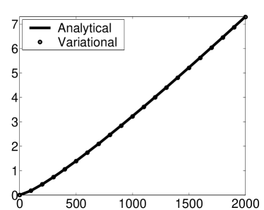
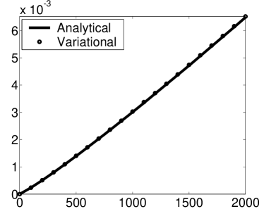
Figure 3: Comparing the WRMS analytical solutions to the variational solutions for the flow of Carreau fluids in straight rigid circular uniform tubes with (a) $n=0.65$, $\mu_{o}=0.1$ Pa.s, $\mu_{i}=0.005$ Pa.s, $\lambda=1.5$ s, $L=0.85$ m and $R=0.09$ m; and (b) $n=0.9$, $\mu_{o}=0.08$ Pa.s, $\mu_{i}=0.001$ Pa.s, $\lambda=2.0$ s, $L=0.5$ m and $R=0.02$ m. In both sub-figures, the vertical axis represents the volumetric flow rate, $Q$, in m³.s^-1 while the horizontal axis represents the pressure drop, $\Delta p$, in Pa. The average percentage relative difference between the analytical and variational solutions for these cases are about 0.37% and 0.60% respectively.

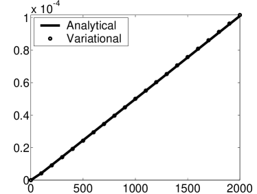
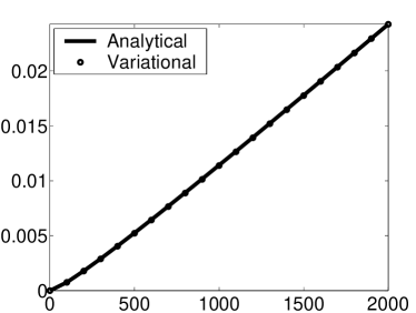
Figure 4: Comparing the WRMS analytical solutions to the variational solutions for the flow of Cross fluids in straight rigid circular uniform tubes with (a) $m=0.83$, $\mu_{o}=0.22$ Pa.s, $\mu_{i}=0.033$ Pa.s, $\lambda=6.65$ s, $L=0.95$ m and $R=0.008$ m; and (b) $m=0.5$, $\mu_{o}=0.15$ Pa.s, $\mu_{i}=0.009$ Pa.s, $\lambda=7.9$ s, $L=1.65$ m and $R=0.027$ m. In both sub-figures, the vertical axis represents the volumetric flow rate, $Q$, in m³.s^-1 while the horizontal axis represents the pressure drop, $\Delta p$, in Pa. The average percentage relative difference between the analytical and variational solutions for these cases are about 0.55% and 0.32% respectively.

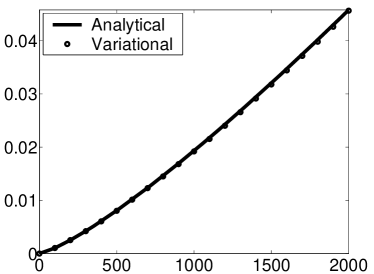
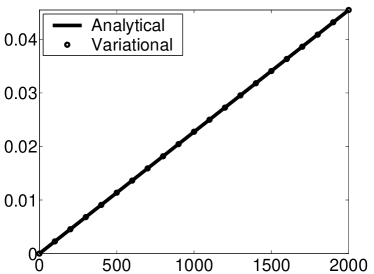
Figure 5: Comparing the WRMS analytical solutions to the variational solutions for the flow of Carreau fluids in straight rigid uniform long thin slits with (a) $n=0.75$, $\mu_{o}=0.17$ Pa.s, $\mu_{i}=0.009$ Pa.s, $\lambda=2.5$ s, $L=1.3$ m, $W=1.0$ m and $B=0.012$ m; and (b) $n=1.0$, $\mu_{o}=0.09$ Pa.s, $\mu_{i}=0.012$ Pa.s, $\lambda=3.0$ s, $L=1.1$ m, $W=1.0$ m and $B=0.015$ m. In both sub-figures, the vertical axis represents the volumetric flow rate, $Q$, in m³.s^-1 while the horizontal axis represents the pressure drop, $\Delta p$, in Pa. The average percentage relative difference between the analytical and variational solutions for these cases are about 0.70% and 0.06% respectively.

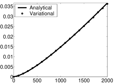
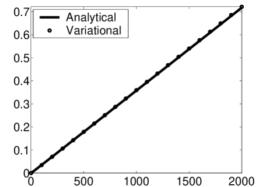
Figure 6: Comparing the WRMS analytical solutions to the variational solutions for the flow of Cross fluids in straight rigid uniform long thin slits with (a) $m=0.45$, $\mu_{o}=0.08$ Pa.s, $\mu_{i}=0.003$ Pa.s, $\lambda=0.75$ s, $L=0.75$ m, $W=1.0$ m and $B=0.005$ m; and (b) $m=0.75$, $\mu_{o}=0.03$ Pa.s, $\mu_{i}=0.005$ Pa.s, $\lambda=5.0$ s, $L=1.25$ m, $W=1.0$ m and $B=0.015$ m. In both sub-figures, the vertical axis represents the volumetric flow rate, $Q$, in m³.s^-1 while the horizontal axis represents the pressure drop, $\Delta p$, in Pa. The average percentage relative difference between the analytical and variational solutions for these cases are about 0.89% and 0.40% respectively.

6 Conclusions

In this paper, a method based on the application of the Weissenberg-Rabinowitsch-Mooney-Schofield (WRMS) equation for the flow of generalized Newtonian fluids in straight rigid circular uniform pipes and its extension to straight rigid long thin uniform slits has been developed and used to find analytical flow solutions for Carreau and Cross fluids which do not have known analytical solutions in those geometries. The main analytical expressions were verified by numerical integration to rule out potential errors in the formality of derivation. The analytical solutions were then thoroughly compared to the solutions of another method, namely the variational approach which is based on the application of the Euler-Lagrange principle and hence it is totally different and independent from the WRMS method. Excellent agreement was obtained in all the investigated cases.

The first thing that has been achieved in this investigation is obtaining fully analytical solutions for the flow of Carreau and Cross fluids in the above mentioned geometries. These solutions provide a better alternative to the use of numerical techniques, which are currently the only available means, since the analytical solutions are easier to obtain, less prone to error and highly accurate. The second is that these analytical solutions provide more support to the previously proposed variational method for obtaining solutions for the flow of generalized Newtonian fluids in confined geometries. In fact this agreement should serve as mutual validation since these methods are totally independent and are based on very different theoretical and mathematical infrastructures and hence they lend support to each other.

It should be remarked that the derivation of the pipe and slit analytical relations for the Carreau model can be easily extended to the more general Carreau-Yasuda model by replacing ‘2’ with ‘$a$’ in the exponents of the Carreau constitutive relation. The WRMS method may also be applied to other non-Newtonian fluid models which do not have analytical solutions. However, in some cases the definite integrals, $I$, may require numerical evaluation by using one of the numerical integration methods such as quadratures, Simpson, trapezium or midpoint integration rules if fully analytical solutions are very difficult or impossible to obtain. Such semi-analytical solutions will not only be much easier to obtain and less prone to errors than their numerical counterparts, but can also be as accurate as any potential analytical solutions for all practical purposes due to the availability of very reliable numerical integration schemes that can be employed. These schemes are easier to implement and more reliable than the alternative numerical techniques like those based on discretization schemes.

7 Nomenclature

$\gamma$	shear rate (s-1)
$\gamma_{w}$	shear rate at conduit wall (s-1)
$\delta$	$\mu_{o}-\mu_{i}$ (Pa.s)
$\lambda$	characteristic time constant (s)
$\mu$	dynamic shear viscosity of generalized Newtonian fluid (Pa.s)
$\mu_{i}$	high-shear viscosity (Pa.s)
$\mu_{o}$	low-shear viscosity (Pa.s)
$\tau$	shear stress (Pa)
$\tau_{B}$	shear stress at slit wall (Pa)
$\tau_{R}$	shear stress at tube wall (Pa)
$\tau_{w}$	shear stress at conduit wall (Pa)
$A_{\parallel}$	area of conduit internal surface (m2)
$B$	slit half height (m)
$f$	$\lambda^{m}\gamma_{w}^{m}$
$F_{\perp}$	force normal to conduit cross section (N)
${}_{2}F_{1}$	hypergeometric function
$g$	$1+f$
$I$	definite integral expression (Pa3.s-1 for pipe and Pa2.s-1 for slit)
$L$	length of conduit (m)
$m$	indicial parameter in Cross model
$n$	flow behavior index in Carreau model
$n^{\prime}$	$n-1$
$\Delta p$	pressure drop (Pa)
$Q$	volumetric flow rate (m3.s-1)
$r$	radius (m)
$R$	tube radius (m)
$v$	fluid velocity in the flow direction (m.s-1)
$W$	slit width (m)
$z$	coordinate of slit smallest dimension (m)

References

- [1] W.J. Cannella; C. Huh; R.S. Seright. Prediction of Xanthan Rheology in Porous Media. SPE Annual Technical Conference and Exhibition, 2-5 October, Houston, Texas, SPE 18089, 1988.
- [2] K.S. Sorbie; P.J. Clifford; E.R.W. Jones. The Rheology of Pseudoplastic Fluids in Porous Media Using Network Modeling. Journal of Colloid and Interface Science, 130(2):508–534, 1989.
- [3] F.J.H. Gijsen; F.N. van de Vosse; J.D. Janssen. Wall shear stress in backward-facing step flow of a red blood cell suspension. Biorheology, 35(4-5):263–279, 1998.
- [4] F.J.H. Gijsen; E. Allanic; F.N. van de Vosse; J.D. Janssen. The influence of the non-Newtonian properties of blood on the flow in large arteries: unsteady flow in a 90∘ curved tube. Journal of Biomechanics, 32(6):601–608, 1999.
- [5] G.C. Georgiou. The time-dependent, compressible Poiseuille and extrudate-swell flows of a Carreau fluid with slip at the wall. Journal of Non-Newtonian Fluid Mechanics, 109(2-3):93–114, 2003.
- [6] X. Lopez; P.H. Valvatne; M.J. Blunt. Predictive network modeling of single-phase non-Newtonian flow in porous media. Journal of Colloid and Interface Science, 264(1):256–265, 2003.
- [7] X. Lopez; M.J. Blunt. Predicting the Impact of Non-Newtonian Rheology on Relative Permeability Using Pore-Scale Modeling. SPE Annual Technical Conference and Exhibition, 26-29 September, Houston, Texas, SPE 89981, 2004.
- [8] F. Abraham; M. Behr; M. Heinkenschloss. Shape optimization in steady blood flow: A numerical study of non-Newtonian effects. Computer Methods in Biomechanics and Biomedical Engineering, 8(2):127–137, 2005.
- [9] F.M.A. Box; R.J. van der Geest; M.C.M. Rutten; J.H.C. Reiber. The Influence of Flow, Vessel Diameter, and Non-Newtonian Blood Viscosity on the Wall Shear Stress in a Carotid Bifurcation Model for Unsteady Flow. Investigative Radiology, 40(5):277–294, 2005.
- [10] J. Chen; X-Y. Lu; W. Wang. Non-Newtonian effects of blood flow on hemodynamics in distal vascular graft anastomoses. Journal of Biomechanics, 39:1983–1995, 2006.
- [11] C.L. Perrin; P.M.J. Tardy; S. Sorbie; J.C. Crawshaw. Experimental and modeling study of Newtonian and non-Newtonian fluid flow in pore network micromodels. Journal of Colloid and Interface Science, 295(2):542–550, 2006.
- [12] A. Jonášová; J. Vimmr. Numerical simulation of non-Newtonian blood flow in bypass models. Proceedings in Applied Mathematics and Mechanics, 79th Annual Meeting of the International Association of Applied Mathematics and Mechanics, Bremen 2008, 8(1):10179–10180, 2008.
- [13] Y.H. Kim; P.J. VandeVord; J.S. Lee. Multiphase non-Newtonian effects on pulsatile hemodynamics in a coronary artery. International Journal for Numerical Methods in Fluids, 58(7):803–825, 2008.
- [14] J. Vimmr; A. Jonás̆ová. On the Modelling of Steady Generalized Newtonian Flows in a 3D Coronary Bypass. Engineering Mechanics, 15(3):193–203, 2008.
- [15] M. Lukáčová-Medvid’ová; A. Zaušková. Numerical modelling of shear-thinning non-Newtonian flows in compliant vessels. International Journal for Numerical Methods in Fluids, 56(8):1409–1415, 2008.
- [16] C. Fisher; J.S. Rossmann. Effect of Non-Newtonian Behavior on Hemodynamics of Cerebral Aneurysms. Journal of Biomechanical Engineering, 131(9):091004(1–9), 2009.
- [17] D.S. Sankar; A.I.Md. Ismail. Two-Fluid Mathematical Models for Blood Flow in Stenosed Arteries: A Comparative Study. Boundary Value Problems, 2009:1–15, 2009.
- [18] A. Hundertmark-Zaušková; M. Lukáčová-Medvid’ová. Numerical study of shear-dependent non-Newtonian fluids in compliant vessels. Computers & Mathematics with Applications, 60(3):572–590, 2010.
- [19] B. Liu; D. Tang. Non-Newtonian Effects on the Wall Shear Stress of the Blood Flow in Stenotic Right Coronary Arteries. International Conference on Computational & Experimental Engineering and Sciences, 17(2):55–60, 2011.
- [20] M.M. Molla; M.C. Paul. LES of non-Newtonian physiological blood flow in a model of arterial stenosis. Medical Engineering & Physics, 34(8):1079–1087, 2012.
- [21] S. Desplanques; F. Renou; M. Grisel; C. Malhiac. Impact of chemical composition of xanthan and acacia gums on the emulsification and stability of oil-in-water emulsions. Food Hydrocolloids, 27(2):401–410, 2012.
- [22] T. Tosco; D.L. Marchisio; F. Lince; R. Sethi. Extension of the Darcy-Forchheimer Law for Shear-Thinning Fluids and Validation via Pore-Scale Flow Simulations. Transport in Porous Media, 96(1):1–20, 2013.
- [23] X. Lopez. Pore-scale modelling of non-Newtonian flow. PhD thesis, Imperial College London, 2004.
- [24] M. Balhoff; D. Sanchez-Rivera; A. Kwok; Y. Mehmani; M. Prodanović. Numerical Algorithms for Network Modeling of Yield Stress and other Non-Newtonian Fluids in Porous Media. Transport in Porous Media, 93(3):363–379, 2012.
- [25] A.R. de Castro; A. Omari; A. Ahmadi-Sénichault; D. Bruneau. Toward a New Method of Porosimetry: Principles and Experiments. Transport in Porous Media, 101(3):349–364, 2014.
- [26] A.H.P. Skelland. Non-Newtonian Flow and Heat Transfer. John Wiley and Sons Inc., 1967.
- [27] T. Sochi. Using the Euler-Lagrange variational principle to obtain flow relations for generalized Newtonian fluids. Rheologica Acta, 53(1):15–22, 2014.
- [28] T. Sochi. Further validation to the variational method to obtain flow relations for generalized Newtonian fluids. Submitted, 2014. arXiv:1407.1534.
- [29] T. Sochi. Variational approach for the flow of Ree-Eyring and Casson fluids in pipes. Submitted, 2014. arXiv:1412.6209.
- [30] T. Sochi. Slip at Fluid-Solid Interface. Polymer Reviews, 51(4):309–340, 2011.
- [31] K.S. Sorbie. Polymer-Improved Oil Recovery. Blackie and Son Ltd, 1991.
- [32] R.I. Tanner. Engineering Rheology. Oxford University Press, 2nd edition, 2000.
- [33] R.G. Owens; T.N. Phillips. Computational Rheology. Imperial College Press, 2002.