A sequential rejection testing method for
high-dimensional regression with correlated variables

Abstract

We propose a general, modular method for significance testing of groups (or clusters) of variables in a high-dimensional linear model. In presence of high correlations among the covariables, due to serious problems of identifiability, it is indispensable to focus on detecting groups of variables rather than singletons. We propose an inference method which allows to build in hierarchical structures. It relies on repeated sample splitting and sequential rejection, and we prove that it asymptotically controls the familywise error rate. It can be implemented on any collection of clusters and leads to improved power in comparison to more standard non-sequential rejection methods. We complete the theoretical analysis with empirical results for simulated and real data.

Keywords and phrases: Familywise error rate; Hierarchical clustering; High-dimensional variable selection; Inheritance procedure; Lasso; Linear model; Minimal true detection; Multiple testing; Sample splitting; Sequential rejection principle; Singleton true detection.

1 Introduction

Error control of false selection or false positive statements based on p-values is a primary goal of statistical inference and an established, broadly used tool in many areas of science. It relies on standard statistical hypothesis testing and procedures which give provable guarantees in presence of multiple, potentially very large scale multiple testing (Westfall,, 1993; Dudoit and van der Laan,, 2007; Efron,, 2010). While being standard in the classical low-dimensional setup, statistical significance testing in the more challenging high-dimensional setting where the number of variables $p$ might be much larger than the sample size $n$ has only received attention recently.

We consider here a linear regression model

$$\mathbf{Y}=\mathbf{X}\beta^{0}+\varepsilon,\ \varepsilon\sim{\cal N}_{n}(0,\sigma^{2}I),$$ (1)

with $n\times p$ design matrix $\mathbf{X}$, $p\times 1$ regression vector $\beta^{0}$ and $n\times 1$ response $\mathbf{Y}$. We allow for high-dimensional scenarios where $p\gg n$. We assume that the regression coefficient vector is sparse with many coefficients of $\beta^{0}$ being equal to zero, that is, the active set of variables

$$S_{0}=\{j;\beta^{0}_{j}\neq 0\}$$

is assumed to be a small subset of $\{1,\ldots,p\}$ corresponding to all variables.

A few methods for assigning $p$-values and constructing confidence intervals for individual parameters $\beta^{0}_{j}\ (j=1,\ldots,p)$ have been suggested (Wasserman and Roeder,, 2009; Meinshausen et al.,, 2009; Bühlmann,, 2013; Zhang and Zhang,, 2014; van de Geer et al.,, 2014; Lockhart et al.,, 2014; Javanmard and Montanari,, 2014), and some of them have been compared against each other in various settings (Bühlmann et al.,, 2014; Dezeure et al.,, 2014). The inferential statements can easily be adjusted for multiplicity, thanks to the methodology and theory in multiple testing (Dudoit and van der Laan,, 2007, cf.). However, and important for practical applications, some major issues in presence of highly correlated variables still need further attention: typically, when $p\gg n$, none or only a few of the individual $\beta^{0}_{j}$’s turn out to be significant which is a consequence of their near non-identifiability (even when some theoretical conditions on well-posedness on the design matrix $\mathbf{X}$ (Bühlmann and van de Geer,, 2011, cf.) hold). However, a group of (correlated) variables is often much better identifiable, but one can then not determine anymore the relevant variables within such a group (Bühlmann et al.,, 2013; Meinshausen,, 2014; Mandozzi and Bühlmann,, 2015).

Thus, our main goal is testing of significance of groups of parameters: for a group or cluster $C\subseteq\{1,\ldots,p\}$ we consider the following null- and alternative hypothesis, respectively:

$$H_{0,C}:\ \beta^{0}_{j}=0\ \mbox{for all}\ j\in C,\ \ \ H_{A,C}:\ \beta^{0}_{j}\neq 0\ \mbox{for at least one}\ j\in C.$$

Given a collection $\mathcal{C}$ of clusters, we propose a general method for obtaining a collection $\mathcal{R}\subset\mathcal{C}$ of rejected clusters such that familywise error rate (FWER) is strongly controlled. That is, for a given nominal level $\alpha\in(0,1)$:

$$\mathbb{P}[\mathcal{R}\subseteq\mathcal{F}]\geq 1-\alpha,$$

where $\mathcal{F}=\{C\in\mathcal{C}\mbox{ s.t. }H_{0,C}\mbox{ is false}\}$ i.e., ${\mathcal{F}}$ is the collection of false null hypotheses. Our new method has the following main features:

• It can be implemented on any collection of clusters $\mathcal{C}$.

• It is modular in the sense that it requires four basic building blocks that have to satisfy certain assumptions.

• Its modular conception allows for a better insight of the procedure’s power and improvements thereof.

We are particularly interested to use the procedure for hierarchically ordered clusters of (correlated) variables. Such a hierarchical structure can be obtained from the output of a hierarchical clustering algorithm: since it operates on the design matrix $\mathbf{X}$ only and does not involve the responses $\mathbf{Y}$, the inference for $\beta^{0}$ remains correct (for fixed design or by conditioning on $\mathbf{X}$). With such a hierarchical cluster tree, our inference method (Sections 2.5 and 4.2) first tests the cluster ${\cal C}=\{1,\ldots,p\}$ containing all the variables (the top node in the tree): if the corresponding null-hypothesis is rejected, we test some refined clusters, and we proceed down the cluster tree, in a sequential manner, until a cluster is not significant anymore. Figures 1 and 2 in Section 5 provide some graphical illustrations. This procedure has the remarkable property that the resolution level of the significant clusters is automatically controlled by the sequential testing method: if the signal is strong (e.g. large absolute values of components of $\beta^{0}$) and the variables are not too highly correlated, one can detect small clusters or even single variables and vice-versa, if the signal isn’t very strong or the variables are highly correlated, only larger groups can be detected as significant.

Relation to other work.

Our proposed method is based on the multi sample splitting method from Meinshausen et al., (2009) and the sequential rejection principle of Goeman and Solari, (2010). It is a generalization and power improvement over the multi sample splitting technique for inference of single variables (Meinshausen et al.,, 2009) and for hierarchically ordered clusters of variables (Mandozzi and Bühlmann,, 2015). The improvement in power is strict, and in analogy to the gain of power of Holm’s procedure (Holm,, 1979) over the Bonferroni adjustment. Thus, even if the increased power might be only small for some datasets, one cannot do worse with the new procedure. The only price to pay is a slightly more complicated algorithm: we provide an implementation in the R-package hdi.

Outline of the paper.

In Section 2 we describe the four basic building blocks of the method and the assumptions that are sufficient to establish in Section 3 its strong FWER control. In Sections 4.1 and 4.2, respectively, we focus on the inference of two specific kinds of cluster collections: singletons and hierarchically ordered clusters. In Section 4.3 we show how logical relationships can be used to improve the power. Finally, we provide in Section 5 a comparison based on empirical results for error control and power, with a focus on minimal true detections, and we apply the new method to a real dataset.

2 A construction based on four building blocks

Our method is based on four basic building blocks that satisfy certain assumptions.

One main ingredient is multi sample splitting. For $b=1,\ldots,B$ where $B$ is the number of repeated sample splitting, the original data of sample size $n$ is split into two disjoint groups, $N_{in}^{(b)}$ and $N_{out}^{(b)}$, i.e., a partition

$$\{1,\dots,n\}=N_{in}^{(b)}\cup N_{out}^{(b)}$$

is randomly chosen. The groups are chosen of equal size if $n$ is even or satisfy $|N_{out}^{(b)}|=|N_{in}^{(b)}|+1$ if $n$ is odd.

The idea is to use data from $N_{in}^{(b)}$ to select a few variables and the other data from $N_{out}^{(b)}$ to perform the statistical hypothesis testing in the low-dimensional submodel with the selected variables from $N_{in}^{(b)}$. The details are described next.

2.1 Screening of variables

We consider variable screening where an estimator $\hat{S}^{(b)}\subseteq\{1,\ldots,p\}$, based on data corresponding to $N_{in}^{(b)}$, is aiming at including all active variables $S_{0}$. A prime example is the Lasso (Tibshirani,, 1996), while a detailed empirical comparison of five popular screening procedures can be found in (Bühlmann and Mandozzi,, 2014). Assume that the screening procedure satisfies the following properties for any sample split $b$:

$$\mbox{(A1) \it{Sparsity property}:}\;|\hat{S}^{(b)}|<n/2.$$

$$\mbox{(A2) \it{$\delta$-Screening property}:}\;\mathbb{P}[\hat{S}^{(b)}\supseteq S_{0}]\geq 1-\delta,\ \mbox{where}\ 0<\delta<1.$$

The sparsity property in (A1) implies that for each sample split $b$ it holds that $|\hat{S}^{(b)}|<|N_{out}^{(b)}|$, a condition which is necessary for applying classical tests as described in Section 2.2 below. The $\delta$-screening property in (A2) ensures that all the relevant variables are retained with high probability (where $\delta>0$ is typically small).

We indicate in Section 3.1 that under some assumptions, the Lasso satisfies (A1) and (A2).

2.2 Testing and p-values

The idea is to perform a classical statistical test on the other half sample from $N_{out}^{(b)}$ in a low-dimensional problem with variables from $\hat{S}^{(b)}$ only.

For each sample split $b$, based on the second half of the sample corresponding to $N_{out}^{(b)}$, consider a testing procedure, e.g. the classical partial F-test (see also Section 3.1), that provides correct p-values $p^{C,(b)}$ for the null hypothesis $H_{0,C\cap\hat{S}^{(b)}}$ for each screened set $\hat{S}^{(b)}$, in the sense that for each nominal level $\alpha\in(0,1)$

$$\mbox{(A3) \it{Correct testing property}:}\mbox{ Under the null hypothesis }H_{0,C\cap\hat{S}^{(b)}}\,\mbox{it holds }\mathbb{P}[p^{C,(b)}\leq\alpha]\leq\alpha.$$

We note that the probability is with respect to the data generating random variables corresponding to the second half $N_{out}^{(b)}$, and the null-hypothesis is fixed with respect to $N_{out}^{(b)}$. Due to the screening property (A2), when $\delta\to 0$, the null-hypothesis $H_{0,C\cap\hat{S}^{(}b)}$ approximates the unconditional hypothesis $H_{0,C}$ which we aim to test for. If $C\cap\hat{S}^{(b)}=\emptyset$ define $p^{C,(b)}=1$. This provides a (correct) p-value $p^{C,(b)}$ for each cluster $C\in\mathcal{C}$ and each sample split $b\in\{1\dots B\}$.

2.3 Multiplicity adjustment

Consider for each sample split $b$ and each cluster $C\in\mathcal{C}$ a multiplicity adjustment procedure $m^{(b)}_{C}:2^{\mathcal{C}}\rightarrow[1,\infty]$ that for each collection $\mathcal{R}$ of rejected clusters provides a multiplicity adjustment $m^{(b)}_{C}(\mathcal{R})\geq 1$ and satisfies the following properties:

$$\mbox{(A4) \it{Monotonicity property}:}\;\mbox{If }\mathcal{R}\subseteq\mathcal{S}\mbox{ then }m^{(b)}_{C}(\mathcal{R})\geq m^{(b)}_{C}(\mathcal{S}).$$

$$\mbox{(A5) \it{Single-step property}:}\;\sum_{C\in\,\mathcal{C}\setminus\mathcal{R}}\frac{1\{C\cap\hat{S}^{(b)}\neq\emptyset\}}{m^{(b)}_{C}(\mathcal{R})}\leq 1,$$

where we define $1/\infty=0$. Such a family of multiplicity adjustments for $b=1,\ldots,B$ are often naturally induced from a global multiplicity adjustment procedure $m_{C}$.

2.4 Aggregation of p-values

Consider a collection of screened sets of variables $\hat{S}^{(b)}$, a cluster $C\in\mathcal{C}$, a collection of p-values $p^{C,(b)}$ for the null-hypothesis $H_{0,C\cap S^{(b)}}$ (which approximates $H_{0,C}$, see comment after (A3)) and a collection of multiplicity adjustments $m_{C}^{(b)}\geq 1$ (we drop here the dependence on ${\cal R}$).

The goal is to aggregate the p-values $p^{C,(1)},\ldots,p^{C,(B)}$ to a single p-value which is adjusted for multiplicity. An aggregation procedure is a monotone increasing function $\mbox{aggr}:[0,1]^{B}\rightarrow[0,1]$. Assume it satisfies the following property:

(A6) Aggregation property: $$\mbox{If }\mathbb{P}[p^{C,(b)}\leq\alpha]\leq\alpha,\ \forall\alpha\in[0,1],\mbox{ then}$$

$$\mathbb{P}[\mbox{aggr}(p^{C,(1)}m_{C}^{(1)},\dots,p^{C,(B)}m_{C}^{(B)})\leq\alpha]$$

$$\leq\frac{\alpha}{B}\sum_{b=1}^{B}\frac{1\{C\cap\hat{S}^{(b)}\neq\emptyset\}}{m_{C}^{(b)}},\ \forall\alpha\in[0,1].$$

2.5 The procedure

Our procedure is based on the four building blocks above. First, we proceed with screening of the variables based on the first half sample from $N_{in}^{(b)}$ (Section 2.1), e.g., in Section 5.1 we use the Lasso with regularization parameter chosen by 10-fold cross-validation (see also Section 3.1). Then, we construct the p-values based on the second half sample from $N_{out}^{(b)}$ by using the partial F-test (Section 2.2 and see also Section 3.1). This leads to a (correct) p-value $p^{C,(b)}$ for each cluster $C\in\mathcal{C}$ and each sample split $b\in\{1\dots B\}$.

The multiplicity adjustment is done sequentially (Section 2.3). Based on a chosen significance level $\alpha\in(0,1)$ and for a collection of currently rejected sets $\mathcal{R}$, define the successor of $\mathcal{R}$ as

$$\mathcal{N}(\mathcal{R})=\{C\in\mathcal{C}\setminus\mathcal{R}\mbox{ s.t. }\mbox{aggr}(p^{C,(1)}m^{(1)}_{C}(\mathcal{R}),\dots,p^{C,(B)}m^{(B)}_{C}(\mathcal{R}))\leq\alpha\}$$

Start from “no rejections” $\mathcal{R}_{0}=\emptyset$, define $\mathcal{R}_{i+1}=\mathcal{R}_{i}\cup\mathcal{N}(\mathcal{R}_{i})$ and $\mathcal{R}_{\infty}=\lim_{i\to\infty}\mathcal{R}_{i}$ (although ${\cal R}_{\infty}$ is never constructed due to finite-ness of all possible subset of the variables). Concrete choices of $m^{(1)}_{C}(\mathcal{R}),\ldots,m^{(B)}_{C}(\mathcal{R})$ are discussed in Section 4.

Finally, we aggregate the p-values as indicated in Section 2.4. Concrete aggregation methods are described in Proposition 1 in Section 3.1.

3 Familywise error control

We show here that the method from Section 2.5 (strongly) controls the FWER at each step $i=0,1,2,\ldots$

Theorem 1.

Assume that (A1)-(A6) hold. Then for any $i\in\mathbb{N}_{0}\cup\infty$

$$\mathbb{P}[\mathcal{R}_{i}\subseteq\mathcal{F}]\geq(1-\delta)^{B}-\alpha,$$

where $\mathcal{F}=\{C\in\mathcal{C}\mbox{ s.t. }C\cap S_{0}\neq\emptyset\}$ is the collection of false null hypotheses.

A proof is given in the Appendix.

3.1 Screening, testing and aggregation: their properties

We discuss here some choices for screening, testing and aggregation which we use in the implementation in the R-package hdi. The issue of sequential multiplicity adjustment is treated separately in Section 4.

For variable screening, we use the Lasso with regularization parameter chosen by 10-fold cross-validation. Theoretical justification of the sparsity and screening property (A1) and (A2) can be derived by assuming a compatibility or restricted eigenvalue condition on the fixed design matrix $\mathbf{X}$ and a beta-min assumption requiring that $\min_{j\in S_{0}}|\beta^{0}_{j}|\gg\sqrt{|S_{0}|\log(p)/n}$ is sufficiently large: we refer to Bühlmann and van de Geer, (2011, Ch. 2.7 and Ch. 6) for the details.

For construction of the p-values (in the low-dimensional setting, due to variable screening in the first half of the sample) we use the partial F-test. Then, assuming fixed design $\mathbf{X}$ and Gaussian errors, condition (A3) holds.

For aggregation of the p-values, ensuring that (A6) holds, we have the following result for two slightly different methods.

Proposition 1.

Denote by $q_{\gamma}(u)$ the empirical $\gamma$-quantile of the values occurring in the components of a vector $u$. The monotone increasing functions $[0,1]^{B}\rightarrow[0,1]$

$$\big{(}\tilde{p}^{(1)},\dots,\tilde{p}^{(B)}\big{)} \longmapsto Q(\gamma)=\min\big{\{}\,1~{},~{}q_{\gamma}\big{(}\tilde{p}^{(1)}/\gamma,\dots,\tilde{p}^{(B)}/\gamma\big{)}\big{\}}$$

$$\big{(}\tilde{p}^{(1)},\dots,\tilde{p}^{(B)}\big{)} \longmapsto \min\big{\{}\,1~{},~{}(1-\log\gamma_{\min})\inf_{\gamma\in(\gamma_{\min},1)}Q(\gamma)\big{\}}$$

satisfy the aggregation property (A6) for any $\gamma,\gamma_{min}\in(0,1)$.

A proof, which was basically given in Meinshausen et al., (2009), can be found in the Appendix.

4 Some concrete methods for multiplicity adjustment

We discuss here the issue of multiplicity adjustment, and justify assumption (A4) and (A5) for different inference procedures.

4.1 Inference of single variables

This first example is paradigmatic for the advantages of the modular approach: a simple improvement of the multiplicity adjustment procedure allows for a better power, basically in the same way as in a low-dimensional setting in (Goeman and Solari,, 2010).

Concretely, we consider the problem of inferring single variables, i.e., the collection of clusters $\mathcal{C}=\{\{i\};i=1,\dots,p\}$. The method proposed in Meinshausen et al., (2009) corresponds to the method of Theorem 1 with the aggregation procedures of Proposition 1 and the following Bonferroni-based (Bonferroni,, 1936; Dunn,, 1961) multiplicity adjustment procedure:

$$m^{(b)}_{\{i\}}(\mathcal{R})=|\hat{S}^{(b)}|.$$ (2)

As the multiplicity adjustments are independent from the (previously) rejected collection of sets, the monotonicity property (A4) is trivially satisfied, while the single-step property (A5) follows from

$$\sum_{C\in\,\mathcal{C}\setminus\mathcal{R}}\frac{1\{C\cap\hat{S}^{(b)}\neq\emptyset\}}{m^{(b)}_{C}(\mathcal{R})}=\sum_{\{i\}\in\,\mathcal{C}\setminus\mathcal{R}}\frac{1\{\{i\}\cap\hat{S}^{(b)}\neq\emptyset\}}{|\hat{S}^{(b)}|}\leq 1.$$

The power of the method can be improved taking instead of (2) the following Bonferroni-Holm-based (Holm,, 1979) multiplicity adjustment procedure:

$$m^{(b)}_{\{i\}}(\mathcal{R})=|\hat{S}^{(b)}\cap(\mathcal{C}\setminus\mathcal{R})|=|\{j\in\hat{S}^{(b)}\mbox{ s.t. }\{j\}\notin\mathcal{R}\}|.$$ (3)

The monotonicity property (A4) is still satisfied since $|\hat{S}^{(b)}\cap(\mathcal{C}\setminus\mathcal{R})|\geq|\hat{S}^{(b)}\cap(\mathcal{C}\setminus\mathcal{S})|$ for $\mathcal{R}\subseteq\mathcal{S}$, whereas

$$\sum_{C\in\,\mathcal{C}\setminus\mathcal{R}}\frac{1\{C\cap\hat{S}^{(b)}\neq\emptyset\}}{m^{(b)}_{C}(\mathcal{R})}=\sum_{\{i\}\in\,\mathcal{C}\setminus\mathcal{R}}\frac{1\{\{i\}\cap\hat{S}^{(b)}\neq\emptyset\}}{|\hat{S}^{(b)}\cap(\mathcal{C}\setminus\mathcal{R})|}=1$$

proves the single step property (A5).

4.2 Inference of hierarchically ordered clusters of variables

When dealing with the challenge of inferring hierarchically ordered clusters of variables, e.g. from the tree-structured output of a hierarchical clustering algorithm, one considers a collection of clusters $\mathcal{C}=\{C_{i}\}_{i}$ where for any two clusters $C_{i},C_{i^{\prime}}\in\mathcal{C}$, either one cluster is a subset of the other, or they have an empty intersection. The method proposed in Mandozzi and Bühlmann, (2015, Section 2), which is based on the procedure of Meinshausen, (2008), corresponds to the one as in Theorem 1 with the aggregation methods of Proposition 1 and the following multiplicity adjustment:

$$m^{(b)}_{C}(\mathcal{R})=\left\{\begin{array}[]{ll}\infty,&\mbox{if }\mbox{anc}(C)\not\subseteq\mathcal{R}\\ \frac{|\hat{S}^{(b)}|}{|\hat{S}^{(b)}\cap C|},&\mbox{if }\mbox{anc}(C)\subseteq\mathcal{R}\mbox{ and }\hat{S}^{(b)}\cap C\neq\emptyset\\ 1,&\mbox{otherwise.}\end{array}\right.$$ (4)

Here, $\mbox{anc}(C)$ denotes the ancestors in a hierarchically ordered cluster tree. To check the monotonicity property (A4), consider $\mathcal{R}\subseteq\mathcal{S}$. For $C\in\mathcal{C}$ with $\mbox{anc}(C)\subseteq\mathcal{R}$ it holds $\mbox{anc}(C)\subseteq\mathcal{S}$ and hence $m^{(b)}_{C}(\mathcal{R})=m^{(b)}_{C}(\mathcal{S})$, while for $C\in\mathcal{C}$ with $\mbox{anc}(C)\not\subseteq\mathcal{R}$ one has $m^{(b)}_{C}(\mathcal{R})=\infty\geq m^{(b)}_{C}(\mathcal{S})$. The single step property (A5) follows from

$$\sum_{C\in\,\mathcal{C}\setminus\mathcal{R}}\frac{1\{C\cap\hat{S}^{(b)}\neq\emptyset\}}{m^{(b)}_{C}(\mathcal{R})} = \frac{1}{|\hat{S}^{(b)}|}\sum_{C\in\,\mathcal{C}\setminus\mathcal{R}\mbox{ s.t. }\mbox{anc}(C)\,\subseteq\,\mathcal{R}}|\hat{S}^{(b)}\cap C|\leq 1,$$

where in the inequality we have used the fact that for two sets in the sum above, one cannot be a subset of the other and hence, by definition of the hierarchy $\mathcal{C}$, they are disjoint.

4.2.1 The inheritance procedure in the high-dimensional setting

In Goeman and Solari, (2010, Section 6.3) and Goeman and Finos, (2012), the authors propose various possibilities on how the sequential rejection principle can be used to improve the power of the hierarchical procedure in Meinshausen, (2008). We consider here the most powerful one, the inheritance procedure of Goeman and Finos, (2012) which we extend to the high-dimensional setting with hierarchical cluster trees. In order to do that, we apply the method of Theorem 1 with the aggregation procedures of Proposition 1 and the following multiplicity adjustment:

$$m^{(b)}_{C}(\mathcal{R})=\left\{\begin{array}[]{ll}\infty,&\mbox{if }\mbox{anc}(C)\not\subseteq\mathcal{R}\\ 1,&\mbox{if }\mbox{anc}(C)\subseteq\mathcal{R}\mbox{ and }\hat{S}^{(b)}\cap C=\emptyset\\ \frac{|\hat{S}^{(b)}|}{|\hat{S}^{(b)}\cap C|}\prod_{D\in\mbox{anc}(C)}n_{D}^{(b)}({\mathcal{R}}),&\mbox{otherwise,}\end{array}\right.$$ (5)

where

$$n_{D}^{(b)}(\mathcal{R})=\frac{1}{|\hat{S}^{(b)}\cap D|}\sum_{E\in\,\mbox{ch}(D)\setminus\mathcal{E}(\mathcal{R})}|\hat{S}^{(b)}\cap E|$$

and

$$\mathcal{E}(\mathcal{R})=\{C\in\mathcal{C}\mbox{ s.t. }\mbox{of}(C)\subseteq{R}\}$$

the set of extinct branches, i.e., the set of hypotheses which have been rejected together with all their offsprings denoted by $\mbox{of}(C)$ (as before, $\mbox{anc}(C)$ denotes the ancestors of cluster $C$). Note that since $n_{D}^{(b)}({\mathcal{R}})\leq 1$ this procedure leads to an uniform improvement over the method of the previous section.

The monotonicity property (A4) follows from the same considerations as above and

$$\mathcal{R}\subseteq\mathcal{S}\Longrightarrow\mathcal{E}(\mathcal{R})\subseteq\mathcal{E}(\mathcal{S})\Longrightarrow n_{D}^{(b)}({\mathcal{R}})\geq n_{D}^{(b)}({\mathcal{S}}).$$

To check that the single step property (A5) holds note that

$$\sum_{C\in\,\mathcal{C}\setminus\mathcal{R}}\frac{1\{C\cap\hat{S}^{(b)}\neq\emptyset\}}{m^{(b)}_{C}(\mathcal{R})}$$

$$= \sum_{C\in\,\mathcal{C}\setminus\mathcal{R}\mbox{ s.t. }\mbox{anc}(C)\,\subseteq\,\mathcal{R}}\frac{|\hat{S}^{(b)}\cap C|}{|\hat{S}^{(b)}|}\prod_{D\in\mbox{anc}(C)}\frac{|\hat{S}^{(b)}\cap D|}{\sum_{E\in\mbox{ch}(D)\setminus\mathcal{E}(\mathcal{R})}|\hat{S}^{(b)}\cap E|}$$

$$= \sum_{C\in\,\mathcal{C}\setminus\mathcal{R}}\frac{\alpha^{(b)}_{C}(\mathcal{R})}{\alpha}$$

where $\alpha^{(b)}_{C}$ is as in Goeman and Finos, (2012, equation (5)) with the weights $w^{(b)}_{C}=|\hat{S}^{(b)}\cap C|$; therefore the single step property follows directly from the considerations in Goeman and Finos, (2012).

4.3 Exploiting logical relationships: Shaffer improvements

Logical relationships between hypothesis can be exploited to improve the power of the sequential rejection procedure. A first example of such an improvement for hierarchically ordered clusters was given in Meinshausen, (2008), while in Goeman and Finos, (2012) the improvement is applied to the inheritance procedure. Since those improvements are based on the considerations of Shaffer, (1986) they are called “Shaffer improvements”. For the high-dimensional setting a possible Shaffer improvement consists of multiplying the multiplicity adjustment $m_{C}^{(b)}(\mathcal{R})$ with the Shaffer factor

$$s_{C}^{(b)}(\mathcal{R})=\max\{m_{C}^{(b)}(\mathcal{U})/m_{C}^{(b)}(\mathcal{R})\,\mbox{ s.t. }C\notin\mathcal{U}\supseteq\mathcal{R},\ \mathcal{U}\mbox{ congruent}\},$$ (6)

where a set $\mathcal{U}\subseteq\mathcal{C}$ is called congruent if, by the logical implications, it can be a complete set of false hypothesis (e.g. for a collection $\mathcal{C}$ of hierarchically ordered hypothesis $\mathcal{U}\subseteq\mathcal{C}$ is congruent if for each $C\in\mathcal{U}$ it holds $\mbox{anc}(C)\subseteq\mathcal{U}$ and at least one offspring leaf node of $C$ is in $\mathcal{U}$).

Note that multiplication with the Shaffer factor never decreases the power of the method since by the monotonicity property (A4), $s_{C}^{(b)}(\mathcal{R})\leq 1$. Moreover $s_{C}^{(b)}(\mathcal{R})=1$ if $\mathcal{R}$ is congruent and since the collection $\mathcal{F}$ of all false hypothesis is congruent, the Shaffer improvement doesn’t affect the validity of equation (8). Finally, for $\mathcal{R}\subseteq\mathcal{S}$,

$$m_{C}^{(b)}(\mathcal{R})s_{C}^{(b)}(\mathcal{R}) = \max\{m_{C}^{(b)}(\mathcal{U})\mbox{ s.t. }C\notin\mathcal{U}\supseteq\mathcal{R},\ \mathcal{U}\mbox{ congruent}\}$$

$$\geq \max\{m_{C}^{(b)}(\mathcal{U})\mbox{ s.t. }C\notin\mathcal{U}\supseteq\mathcal{S},\ \mathcal{U}\mbox{ congruent}\}$$

$$= m_{C}^{(b)}(\mathcal{S})s_{C}^{(b)}(\mathcal{S})$$

and hence the Shaffer improvement doesn’t affect the validity of equation (7) neither.

We want to apply this Shaffer improvement to the inheritance procedure described in Section 4.2.1. Following the same reasoning as in Goeman and Finos, (2012, Section 6), with the weights $w_{C}^{(b)}=|\hat{S}^{(b)}\cap C|$ we get the Shaffer factor

$$s_{C}^{(b)}(\mathcal{R})=\left\{\begin{array}[]{ll}\frac{w_{C}^{(b)}+u_{C}^{(b)}-v_{C}^{(b)}}{w_{C}^{(b)}+u_{C}^{(b)}},&\mbox{if }C\notin\mathcal{R},\mbox{si}(C)\subseteq\mathcal{L}\setminus\mathcal{R}\\ 1,&\mbox{otherwise,}\end{array}\right.$$

where $\mbox{si}(C)=\mbox{ch}\{\mbox{pa}(C)\}\setminus\{C\}$ denotes the siblings of $C$, $\mathcal{L}\subset\mathcal{C}$ denotes the collection of leaf nodes, $u_{C}^{(b)}=\sum_{D\in\mbox{si}(C)}w_{D}^{(b)}$ and $v_{C}^{(b)}=\min_{D\in\mbox{si}(C)}w_{D}^{(b)}$. If $\mathcal{C}$ is a binary tree the Shaffer factor becomes

$$s_{C}^{(b)}(\mathcal{R})=\left\{\begin{array}[]{ll}\frac{|\hat{S}^{(b)}\cap C|}{|\hat{S}^{(b)}\cap C|+|\hat{S}^{(b)}\cap\,\mbox{si}(C)|},&\mbox{if }C\notin\mathcal{R},\mbox{si}(C)\subseteq\mathcal{L}\setminus\mathcal{R}\\ 1,&\mbox{otherwise.}\end{array}\right.$$

Unlike as for the inheritance procedure in (5), the Shaffer factor (6) for the procedure in (4) is always 1. Nevertheless, a possibility how to exploit logical relationships to improve the power of the procedure (4) for binary trees, which provides a Shaffer improvement very similar to the one above, is illustrated in Mandozzi and Bühlmann, (2015).

5 Empirical results

5.1 Implementation of the methods and considered scenarios

In this section we compare the performance of the four methods illustrated in Sections 4.1 and 4.2 and refined in Section 4.3, i.e. single variable method with Bonferroni multiplicity adjustment (2), hierarchical method with Bonferroni-based adjustment (4) along with Shaffer improvement as in Mandozzi and Bühlmann, (2015), single variable method with Bonferroni-Holm multiplicity adjustment (3) and hierarchical method with inheritance procedure (5) along with Shaffer improvement (6). In the following we refer to the first two methods as the “non-sequential methods” (strictly seen, the hierarchical method with Bonferroni-based adjustment is actually sequential, but there previous rejections are not used to improve subsequent multiplicity corrections) and the latter two methods as the “sequential methods”.

We consider the same implementation of the methods and the same scenarios (with exactly the same sample splits) as in Mandozzi and Bühlmann, (2015), although here we use only standard hierarchical clustering for the hierarchical methods. Concretely, the following choices have been made for implementation:

• construction of the clusters with standard hierarchical clustering (using the R-function hclust) with distance between two covariables equal to 1 minus the absolute correlation between the covariables, and using complete linkage;

• screening with the Lasso (Tibshirani,, 1996) with regularization parameter chosen by 10-fold cross-validation;

• $B=50$ sample splits (for each scenario exactly the same splits as in Mandozzi and Bühlmann, (2015));

• for aggregation, the p-values $P_{h}^{C}$ in Proposition 1 are computed over a grid of $\gamma$-values between $\gamma_{min}=0.05$ and $1$ with grid-steps of size $0.025$;

• nominal significance level $\alpha=5\%$.

The following scenarios are considered (for the details we refer to Mandozzi and Bühlmann, (2015)):

• 42 scenarios based on 7 designs;

• for each design we consider 6 settings by varying the number of variables $p$ in the model and the signal to noise ratio defined by $\mbox{SNR}=\sqrt{(\beta^{0})^{T}\mathbf{X}^{T}\mathbf{X}\beta^{0}n^{-1}\sigma^{-2}}$, namely for $p=200$ we use $\mbox{SNR}=4$ and $\mbox{SNR}=8$, for $p=500$ we use $\mbox{SNR}=8$ and $\mbox{SNR}=16$ and for $p=1000$ we use $\mbox{SNR}=16$ and $\mbox{SNR}=32$;

• 3 designs based on synthetic data (“equi correlation”, “high correlation within small blocks” and “high correlation within large blocks”) and 4 designs based on semi-real data (“Riboflavin with normal correlation”, “Breast with normal correlation”, “Riboflavin with high correlation”, “Breast with high correlation”);

• sparsity $s_{0}=6$ for the two “Riboflavin”-designs and $s_{0}=10$ for the other five designs.

5.2 Familywise error rate control (FWER)

For each of the 42 scenarios described in Section 5.1 we consider exactly the same 100 independent simulation runs as in Mandozzi and Bühlmann, (2015, Section 4.2.2) by varying only the synthetic noise term $\varepsilon$ and count the number where at least one false selection is made. According to Theorem 1, we expect this number to be at most $100\alpha=5$ ($\alpha=0.05$). The results for the Bonferroni-based methods can be seen in Mandozzi and Bühlmann, (2015, Table 1): FWER control holds for 40 of the 42 scenarios and in 37 scenarios there is no false selection at all.

The results for the methods with sequential rejection are very similar, the only differences being that for the “high correlation within small blocks”-design with $p=500$ and $\mbox{SNR}=8$ the number of runs with at least a false selection increases (compared to Bonferroni-type methods) from 7 to 9 for the single variable method, and from 7 to 13 for the hierarchical method, respectively; for the same design with $p=1000$ and $\mbox{SNR}=16$ the number of runs with at least a false selection increases from 5 to 6 for both the single variable and hierarchical method. For all other scenarios, inclusively the “high correlation within large blocks”-design with $p=200$ and $\mbox{SNR}=4$, where the non-sequential hierarchical method slightly failed to control FWER (6 runs with at least a false detection), the sequential methods exhibit the same FWER control as their non-sequential counterparts.

Summarizing, FWER holds for all four methods in 39 out of 42 scenarios and the designs where it doesn’t fully hold are “high correlation within small blocks” and “high correlation within large blocks”, which is not surprising since each active predictor is highly correlated with a false variable from $S_{0}^{c}$ and hence it is rather difficult for our screening method (the Lasso) to guarantee that $\hat{S}\supseteq S_{0}$.

5.3 Power

For measuring the power we consider four different aspects: the one-dimensional statistics defined in Mandozzi and Bühlmann, (2015, Section 4.2.1) as “Performance 1” and “Performance 2” (see below), the number of minimal true detections (MTDs, i.e., smallest significant groups of variables of any cardinality, containing at least one active variable, see below) and singleton true detections (STDs, i.e., MTDs with cardinality 1). Concretely, a cluster is said to be a MTD if it satisfies all of the following:

• $C$ is a significant cluster, e.g., has p-value $<5\%$ (“Detection”);

• There is no significant sub-cluster $D\subset C$ (“Minimal”);

• $C\notin\mathcal{T}_{0}$, i.e., there is at least one active variable in $C$ (“True”);

and we define:

Performance 1 $$= \frac{1}{|S_{0}|}\sum_{\mbox{MTD C}}\frac{1}{|C|},$$

Performance 2 $$= \frac{1}{|S_{0}|}\sum_{\mbox{MTD C with }|C|\leq 20}\frac{1}{2}\Big{(}\frac{1}{|C|}+1\Big{)}.$$

For each of the 42 scenarios outlined in Section 5.1, we consider exactly the same 100 independent simulation runs obtained in Mandozzi and Bühlmann, (2015, Section 4.2.3-4) by varying the synthetic noise term $\varepsilon$ and the synthetic regression vector $\beta^{0}$. We then calculate the average Performance 1, Performance 2, number of MTDs and number STDs, over the 100 simulation runs. The results are shown in Table 1 for low SNR and Table 2 for high SNR (for the single variable methods each MTD is an STD and by definition Performance 2 is the same as Performance 1).

		low SNR
Design	$p$	# MTDs				# STDs		Perf 1				Perf 2
		SB	SH	HB	HSR	HB	HSR	SB	SH	HB	HSR	HB	HSR
	200	4.79	5.00	5.40	5.59	4.34	4.55	47.9	50.0	44.2	46.3	46.1	48.1
equi	500	3.97	4.13	4.74	4.84	3.73	3.84	39.7	41.3	37.7	38.7	38.3	39.3
corr	1000	1.77	1.79	2.54	2.54	1.73	1.73	17.7	17.9	17.4	17.4	17.6	17.6
	200	4.45	4.78	6.85	7.12	4.36	4.84	44.5	47.8	53.7	57.5	60.7	64.0
small	500	3.15	3.33	5.18	5.27	3.15	3.42	31.5	33.3	38.3	40.1	44.2	45.5
blocks	1000	1.31	1.35	2.53	2.57	1.31	1.37	13.1	13.5	15.1	15.6	17.2	17.7
	200	0.29	0.30	6.50	6.50	0.28	0.28	2.9	3.0	6.7	6.7	31.3	31.3
large	500	0.06	0.06	2.76	2.76	0.06	0.06	0.6	0.6	1.1	1.1	1.1	1.1
blocks	1000	0.00	0.00	0.60	0.60	0.00	0.00	0.0	0.0	0.1	0.1	0.1	0.1
Riboflavin	200	1.41	1.43	2.41	2.46	1.33	1.35	23.5	23.8	23.4	23.8	25.2	25.7
normal	500	0.90	0.90	1.84	1.85	0.77	0.79	15.0	15.0	13.5	13.8	14.2	14.5
corr	1000	0.72	0.73	1.60	1.63	0.63	0.66	12.0	12.2	10.8	11.2	11.0	11.4
Breast	200	4.05	4.16	5.00	5.11	3.84	3.94	40.5	41.6	39.5	40.6	41.6	42.9
normal	500	3.95	4.02	5.04	5.11	3.82	3.87	39.5	40.2	38.8	39.3	39.6	40.2
corr	1000	3.30	3.34	4.25	4.27	3.10	3.13	33.0	33.4	31.2	31.5	31.7	31.9
Riboflavin	200	1.44	1.49	2.96	2.96	1.41	1.44	24.0	24.8	26.0	26.4	31.8	32.1
high	500	1.72	1.79	2.95	2.98	1.69	1.72	28.7	29.8	29.9	30.4	32.8	33.3
corr	1000	1.51	1.51	2.54	2.56	1.49	1.52	25.2	25.2	25.3	25.8	25.7	26.1
Breast	200	3.98	4.10	5.91	5.95	3.87	3.91	39.8	41.0	41.2	41.6	46.1	46.6
high	500	5.13	5.22	6.51	6.56	4.87	4.93	51.3	52.2	49.9	50.4	51.7	52.3
corr	1000	4.73	4.77	5.95	5.98	4.64	4.67	47.3	47.7	47.0	47.3	48.3	48.6
Average		2.51	2.58	4.00	4.06	2.40	2.48	27.5	28.3	28.1	28.8	31.3	31.9

Table 1: Number of MTDs, number of STDs, Performance 1 in % and Performance 2 in %, averaged over 100 simulation runs, for single variable method with Bonferroni (SB), single variable method with Bonferroni-Holm (SH), hierarchical method with Bonferroni (HB) and hierarchical method with sequential rejection induced by the inheritance procedure (HSR). Scenarios with low SNR.

		high SNR
Design	$p$	# MTDs				# STDs		Perf 1				Perf 2
		SB	SH	HB	HSR	HB	HSR	SB	SH	HB	HSR	HB	HSR
	200	9.77	9.83	9.79	9.80	9.73	9.74	97.7	98.3	97.4	97.5	97.4	97.5
equi	500	7.28	7.38	7.63	7.67	7.18	7.24	72.8	73.8	72.0	72.5	72.1	72.6
corr	1000	2.81	2.84	3.50	3.50	2.78	2.78	28.1	28.4	27.9	27.9	28.1	28.1
	200	9.18	9.31	9.98	10.00	9.29	9.48	91.8	93.1	96.3	97.4	98.1	98.7
small	500	6.99	7.03	8.05	8.14	7.02	7.15	69.9	70.3	73.5	74.7	76.4	77.4
blocks	1000	2.26	2.27	3.40	3.41	2.26	2.28	22.6	22.7	24.3	24.5	26.3	26.5
	200	2.17	2.26	9.58	9.58	2.13	2.14	21.7	22.6	27.9	28.0	61.4	61.4
large	500	1.17	1.20	5.38	5.38	1.15	1.15	11.7	12.0	12.6	12.6	13.2	13.2
blocks	1000	0.43	0.45	1.11	1.11	0.43	0.43	4.3	4.5	4.4	4.4	4.4	4.4
Riboflavin	200	3.39	3.46	3.89	3.92	3.33	3.34	56.5	57.7	56.3	56.5	58.7	59.1
normal	500	2.24	2.25	2.90	2.90	2.15	2.15	37.3	37.5	36.4	36.4	36.9	36.9
corr	1000	0.98	1.00	1.83	1.83	0.96	0.96	16.3	16.7	16.2	16.2	16.3	16.3
Breast	200	8.65	8.70	8.89	8.93	8.60	8.65	86.5	87.0	86.4	86.8	87.2	87.7
normal	500	6.81	6.86	7.33	7.35	6.72	6.74	68.1	68.6	67.6	67.8	68.3	68.5
corr	1000	3.95	3.97	4.81	4.84	3.79	3.82	39.5	39.7	38.1	38.4	38.4	38.7
Riboflavin	200	3.86	3.97	4.79	4.83	3.82	3.86	64.3	66.2	66.0	66.7	69.4	70.1
high	500	3.69	3.72	4.40	4.43	3.65	3.68	61.5	62.0	61.8	62.3	63.7	64.2
corr	1000	2.48	2.51	3.24	3.27	2.43	2.45	41.3	41.8	40.7	41.0	41.1	41.4
Breast	200	9.09	9.15	9.59	9.61	9.09	9.14	90.9	91.5	91.9	92.3	93.8	94.1
high	500	7.75	7.82	8.38	8.40	7.71	7.72	77.5	78.2	77.8	78.0	78.9	79.1
corr	1000	5.85	5.89	6.73	6.76	5.72	5.75	58.5	58.9	57.5	57.9	58.1	58.5
Average		4.80	4.85	5.96	5.98	4.76	4.79	53.3	53.9	54.0	54.3	56.6	56.9

Table 2: Number of MTDs, number of STDs, Performance 1 in % and Performance 2 in %, averaged over 100 simulation runs, for single variable method with Bonferroni (SB), single variable method with Bonferroni-Holm (SH), hierarchical method with Bonferroni (HB) and hierarchical method with sequential rejection induced by the inheritance procedure (HSR). Scenarios with high SNR.

Considering both low and high SNR, the methods with sequential rejection improve the considered power measures in comparison to the analogous method without sequential rejection in 207 out of 252 cases, the absolute improvement being at least 0.05 for MTDs and STDs, and at least 0.5 percent for Performance 1 and Performance 2 in 133 cases out of 252 cases. For better interpretation of these results: an absolute improvement of 0.05 MTDs (resp. STDs) basically means that in one out of 20 runs one more MTD (resp. STD) could be detected. Averaging over all scenarios, the improvement given by the sequential rejection procedures lies between 0.04 and 0.06 for MTDs and STDs, and between 0.5 and 0.7 percent for Performance 1 and Performance 2. The biggest gain with sequential rejection can be found in the “high correlation within small blocks”-design with $p=200$ and low SNR: it consists of 0.48 more STDs, 0.33 more MTDs and an absolute increase of 3.8 percent of Performance 1 and 3.3 percent of Performance 2, respectively. This basically means that in half of the runs the method with sequential rejection could find one STD more and in one third of the runs it could find one MTD more. Other particularly favorable scenarios for an improvement with sequential rejection are the “equi correlation”-design and the “breast normal corr”-design, both with $p=200$ and low SNR and the “high correlation within small blocks”-design with high SNR and $p=200$, resp. $p=500$.

In general, the improvement given by the sequential rejection procedures decreases with increasing number $p$ of covariables and is substantial only when the power of the method without sequential rejection is intermediate. These empirical findings are not surprising, since looking at how the methods are defined and in particular at the equations (2), (3), (4) and (5), we conclude that an improvement with the sequential rejection methods is only possible if the related non-sequential method provides at least an STD (and gets more likely the more STDs are provided by the non-sequential method). Moreover, an improvement with sequential rejection is more likely to happen when the number $|\hat{S}|$ of screened variables is small.

For a better illustration of what kind of an improvement is possible using sequential rejection, we show in Figures 1 and 2 the dendrograms (in gray) for a paradigmatic simulation run of the “equi correlation”- and the “high correlation within small blocks”-design, respectively, both with $p=200$ and $\mbox{SNR}=4$.

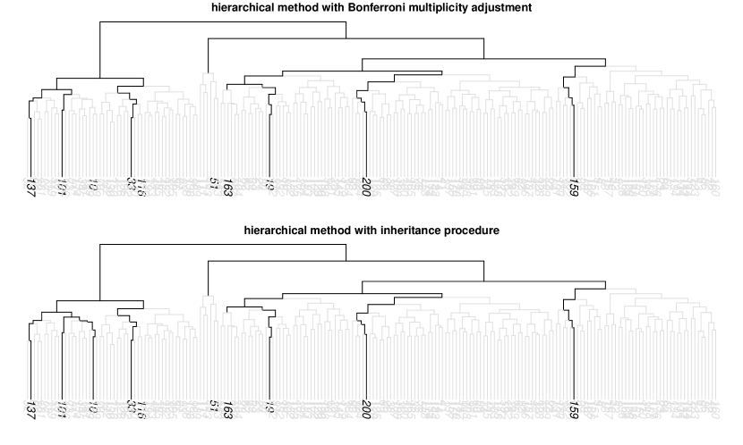
Figure 1: Dendrograms for a paradigmatic simulation run of the “equi correlation”-design with $p=200$ and $\mbox{SNR}=4$. The active variables are labeled in black and the truly detected non-zero variables along the hierarchy are depicted in black.

Figure 1 illustrates that sequential rejection allows the detection of a further singleton, increasing the number of STDs from 6 to 7 and the number of MTDs 8 to 9. In Figure 2 sequential rejection allows to detect a singleton that could previously only be detected together with another non-relevant variable in a cluster of cardinality 2, increasing the number of true STDs from 4 to 5 (while the number of MTDs remains to be 6).

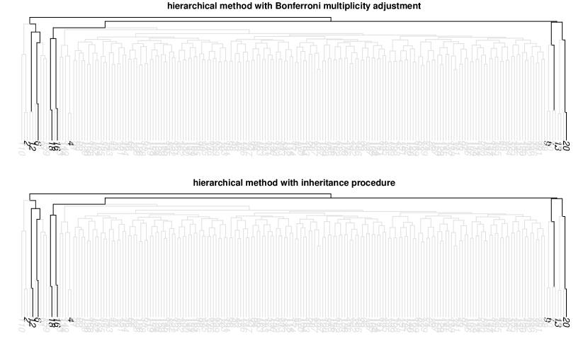
Figure 2: Dendrograms for a paradigmatic simulation run of the “high correlation within small blocks”-design with $p=200$ and $\mbox{SNR}=4$. The active variables are labeled in black and the truly detected non-zero variables along the hierarchy are depicted in black.

Finally, we have performed a simulation with the same scenarios (and the same sample splits) as in Mandozzi and Bühlmann, (2015, Section 4.3), i.e. “small blocks”-designs and “large blocks”-designs with 8 different correlations $\rho\in\{0,0.4,0.7,0.8,0.85,0.9,0.95,0.99\}$. The full results are shown in Tables 3 and 4 in the Appendix. While the methods with sequential rejection control the FWER in exactly the same scenarios where it is also controlled by the non-sequential methods, they increase the average number of MTDs from 5.51 to 5.62 for the single variable method, and from 8.11 to 8.18 for the hierarchical method, and the number of STDs for the hierarchical method from 5.44 to 5.55, with improvements for a single scenario up to 0.48 MTDs and 0.56 STDs (averaged over 100 runs).

The empirical results can be summarized as follows. The methods with sequential rejection essentially controls the FWER in the same way as the non-sequential methods. Regarding power, sequential rejection allows for improvements, to a similar extent for the single variable and the hierarchical procedures. As already noted in Mandozzi and Bühlmann, (2015), for the non-sequential methods, the hierarchical methods have similar STDs as the single variable methods but allow for substantially more MTDs. Thus, our proposed hierarchical method with the inheritance procedure can be seen as the best of the considered methods.

5.4 Real data application: Motif Regression

We consider here a problem of motif regression (Conlon et al.,, 2003) from computational biology. We apply the four methods described above, plus the two hierarchical methods (with and without sequential rejection) using the recently proposed canonical correlation clustering of of Bühlmann et al., (2013), to a real dataset with $n=287$ and $p=195$, used in Meinshausen, (2008, Section 4.3) and Mandozzi and Bühlmann, (2015, Section 4.4). The sequential rejection methods detects exactly the same significant structures as non-sequential methods, namely a single variable and a cluster containing 165 variables (the latter can be detected only with the hierarchical method with canonical correlation clustering). This can barely be considered as surprising, as with only one STD by the non-sequential methods, further improvements by the sequential methods are rather unlikely (see Section 5.3 for more explanation and empirical evidence).

6 Conclusions

We propose a general sequential rejection testing method for clusters and single variables in a high-dimensional linear model. In presence of high correlations among the covariables, due to serious problems of identifiability, it is essentially mandatory to focus on detecting significant groups of variables rather than single individual covariates. Our method asymptotically controls the familywise error rate (FWER), while, as a consequence of its modular structure, allowing for unburdened power optimization. We provide an implementation in the R-package hdi.

We use and study the procedure for inference of single variables but much more importantly, for hierarchically ordered clusters of variables. With the latter, we establish a powerful scheme for meaningful inference in a high-dimensional regression model, much beyond considering single variables only. Our presented mathematical analysis on control of the FWER and power improvement is complemented by empirical results based on semi-real and simulated data confirming the theoretical results.

7 Appendix

7.1 Proof of Theorem 1

Proof.

We show that the procedure satisfies monotonicity and single-step conditions as required by Goeman and Solari, (2010, Theorem 1), i.e.

$$\mathcal{R}\subseteq\mathcal{S}\Rightarrow\mathcal{N}(\mathcal{R})\subseteq\mathcal{N}(\mathcal{S})\cup\mathcal{S}$$ (7)

$$\mathbb{P}[\mathcal{N}(\mathcal{F})\subseteq\mathcal{F}]\geq(1-\delta)^{B}-\alpha.$$ (8)

Assume $\mathcal{R}\subseteq\mathcal{S}$ and $C\in\mathcal{N}(\mathcal{R})$. Then by definition $\mbox{aggr}(p^{C,(1)}m^{(1)}_{C}(\mathcal{R}),\dots,p^{C,(B)}m^{(B)}_{C}(\mathcal{R}))\leq\alpha$. The monotonicity property (A4) of the multiplicity adjustment and the fact that the aggregation procedure is monotone increasing imply

$$\mbox{aggr}(p^{C,(1)}m^{(1)}_{C}(\mathcal{S}),\dots,p^{C,(B)}m^{(B)}_{C}(\mathcal{S}))\leq\mbox{aggr}(p^{C,(1)}m^{(1)}_{C}(\mathcal{R}),\dots,p^{C,(B)}m^{(B)}_{C}(\mathcal{R}))$$

and hence either $C\in\mathcal{S}$ or $C\in\mathcal{N}(\mathcal{S})$ which proves (7). Consider the event

$$\mathcal{A}=\{\,\hat{S}^{(b)}\supseteq S_{0},\forall\,b=1\dots B\,\}$$

where all screenings are satisfied. Because of the $\delta$-screening assumption (A2) it holds $\\ P(\mathcal{A})\geq(1-\delta)^{B}$ and hence

$$\mathbb{P}[\mathcal{N}(\mathcal{F})\not\subseteq\mathcal{F}] = \mathbb{P}[\mathcal{N}(\mathcal{F})\not\subseteq\mathcal{F}\,|\,\mathcal{A}]\,\mathbb{P}(\mathcal{A})+\mathbb{P}[\mathcal{N}(\mathcal{F})\not\subseteq\mathcal{F}\,|\,\mathcal{A}^{c}]\,\mathbb{P}(\mathcal{A}^{c})$$

$$\leq \mathbb{P}[\mathcal{N}(\mathcal{F})\not\subseteq\mathcal{F}\,|\,\mathcal{A}]+(1-(1-\delta)^{B}).$$

Since

$$\mathbb{P}[\mathcal{N}(\mathcal{F})\not\subseteq\mathcal{F}\,|\,\mathcal{A}] \leq \mathbb{P}[\bigcup_{\mathcal{C}\setminus\mathcal{F}}\{\mbox{aggr}(p^{C,(1)}m^{(1)}_{C}(\mathcal{F}),\dots,p^{C,(B)}m^{(B)}_{C}(\mathcal{F}))\leq\alpha\}]$$

$$\leq \sum_{\mathcal{C}\setminus\mathcal{F}}\mathbb{P}[\mbox{aggr}(p^{C,(1)}m^{(1)}_{C}(\mathcal{F}),\dots,p^{C,(B)}m^{(B)}_{C}(\mathcal{F}))\leq\alpha\}]$$

$$\stackrel{{\scriptstyle(A3)(A6)}}{{\leq}} \sum_{\mathcal{C}\setminus\mathcal{F}}\frac{\alpha}{B}\sum_{b=1}^{B}\frac{1\{C\cap\hat{S}^{(b)}\neq 0\}}{m^{(b)}_{C}(\mathcal{F})}=\frac{\alpha}{B}\sum_{b=1}^{B}\sum_{\mathcal{C}\setminus\mathcal{F}}\frac{1\{C\cap\hat{S}^{(b)}\neq 0\}}{m^{(b)}_{C}(\mathcal{F})}$$

$$\stackrel{{\scriptstyle(A5)}}{{\leq}} \frac{\alpha}{B}\sum_{b=1}^{B}1\leq\alpha$$

we conclude $\mathbb{P}[\mathcal{N}(\mathcal{F})\subseteq\mathcal{F}]=1-\mathbb{P}[\mathcal{N}(\mathcal{F})\not\subseteq\mathcal{F}]\geq 1-(\alpha+(1-(1-\delta)^{B}))=(1-\delta)^{B}-\alpha$ which proves (8). ∎

7.2 Proof of Proposition 1

Proof.

The proof was basically given in the Appendix of Meinshausen et al., (2009).
In the following we omit the function $\min\{1,\cdot\}$ from the definition of $Q(\gamma)$ in order to simplify the notation (this is possible since the level $\alpha$ is smaller than 1). Define for $u\in(0,1)$ the function

$$\pi(u):=\frac{1}{B}\sum_{b=1}^{B}1\{\tilde{p}^{(b)}\leq u\}.$$

Then it holds

$$Q(\gamma)\leq\alpha \Longleftrightarrow q_{\gamma}(\tilde{p}^{(1)}/\gamma,\dots,\tilde{p}^{(B)}/\gamma)\leq\alpha\Longleftrightarrow q_{\gamma}(\tilde{p}^{(1)},\dots,\tilde{p}^{(B)})\leq\alpha\gamma$$

$$\Longleftrightarrow \sum_{b=1}^{B}1\{\tilde{p}^{(b)}\leq\alpha\gamma\}\geq B\gamma\Longleftrightarrow\pi(\alpha\gamma)\geq\gamma.$$

Thus,

$$\mathbb{P}(Q(\gamma)\leq\alpha) = \mathbb{E}(1\{Q(\gamma)\leq\alpha\})=\mathbb{E}(1\{\pi(\alpha\gamma)\geq\gamma\})\leq\frac{1}{\gamma}\mathbb{E}(\pi(\alpha\gamma))$$

$$= \frac{1}{\gamma}\mathbb{E}\Big{(}\frac{1}{B}\sum_{b=1}^{B}1\{\tilde{p}^{(b)}\leq\alpha\gamma\}\Big{)}=\frac{1}{\gamma}\frac{1}{B}\sum_{b=1}^{B}\mathbb{E}\Big{(}1\{\tilde{p}^{(b)}\leq\alpha\gamma\}\Big{)}$$

$$= \frac{1}{\gamma}\frac{1}{B}\sum_{b=1}^{B}\mathbb{P}(\tilde{p}^{(b)}\leq\alpha\gamma)\leq\frac{1}{\gamma}\frac{1}{B}\sum_{b=1}^{B}\frac{\alpha\gamma}{m^{(b)}}1\{C\cap\hat{S}^{(b)}\neq\emptyset\}$$

$$= \frac{\alpha}{B}\sum_{b=1}^{B}\frac{1\{C\cap\hat{S}^{(b)}\neq\emptyset\}}{m^{(b)}},$$

where the first inequality is a consequence of the Markov inequality and the last inequality is a consequence of the assumptions that $P(\tilde{p}^{(b)}\leq\alpha)=P(p^{(b)}m^{(b)}\leq\alpha)\leq\alpha/m^{(b)}$ and the definition $\tilde{p}^{(b)}=1$ for $C\cap\hat{S}^{(b)}=\emptyset$.
For a random variable $U$ taking values in $[0,1]$,

$$\sup_{\gamma\in(\gamma_{\min},1)}\frac{1\{U\leq\alpha\gamma\}}{\gamma}=\left\{\begin{array}[]{ll}0,&U\geq\alpha\\ \alpha/U,&\alpha\gamma_{\min}\leq U<\alpha\\ 1/\gamma_{\min},&U\leq\alpha\gamma_{\min}.\\ \end{array}\right.$$

and if $U$ has an uniform distribution on $[0,1]$

$$\mathbb{E}\Big{(}\sup_{\gamma\in(\gamma_{\min},1)}\frac{1\{U\leq\alpha\gamma\}}{\gamma}\Big{)} = \int_{0}^{\alpha\gamma_{\min}}\gamma_{\min}^{-1}dx+\int_{\alpha\gamma_{\min}}^{\alpha}\alpha x^{-1}dx$$

$$= \gamma_{\min}^{-1}x\big{|}_{x=0}^{x=\alpha\gamma_{\min}}+\alpha\log x\big{|}_{x=\alpha\gamma_{\min}}^{x=\alpha}$$

$$= \alpha+\alpha(\log\alpha-\log(\alpha\gamma_{\min}))$$

$$= \alpha\big{(}1-\log\frac{\alpha}{\alpha\gamma_{\min}}\big{)}=\alpha(1-\log\gamma_{\min}).$$

We apply this using as $U$ the uniform distributed $\tilde{p}^{(b)}/m^{(b)}=p^{(b)}$ for $C\cap S^{(b)}\neq\emptyset$ and obtain

$$\mathbb{E}\Big{(}\sup_{\gamma\in(\gamma_{\min},1)}\frac{1\{\tilde{p}^{(b)}/m^{(b)}\leq\alpha\gamma\}}{\gamma}\Big{)}\leq\alpha(1-\log\gamma_{\min}),$$

and similarly as above

$$\mathbb{P}\big{(}\inf_{\gamma\in(\gamma_{\min},1)}Q(\gamma)\leq\alpha\big{)} = \mathbb{E}\Big{(}\sup_{\gamma\in(\gamma_{\min},1)}1\{\pi(\alpha\gamma)\geq\gamma\}\Big{)}$$

$$\leq \mathbb{E}\Big{(}\sup_{\gamma\in(\gamma_{\min},1)}\frac{1}{B}\sum_{b=1}^{B}\frac{1\{\tilde{p}^{(b)}\leq\alpha\gamma\}}{\gamma}\Big{)}$$

$$= \mathbb{E}\Big{(}\sup_{\gamma\in(\gamma_{\min},1)}\frac{1}{B}\sum_{b=1}^{B}\frac{1\{\tilde{p}^{(b)}\leq\alpha\gamma\}1\{C\cap S^{(b)}\neq\emptyset\}}{\gamma}\Big{)}$$

$$\leq \frac{1}{B}\sum_{b=1}^{B}\mathbb{E}\Big{(}\sup_{\gamma\in(\gamma_{\min},1)}\frac{1\{\tilde{p}^{(b)}/m^{(b)}\leq\alpha\gamma/m^{(b)}\}1\{C\cap S^{(b)}\neq\emptyset\}}{\gamma}\big{)}\Big{)}$$

$$\leq (1-\log\gamma_{\min})\frac{\alpha}{B}\sum_{b=1}^{B}\frac{1\{C\cap S^{(b)}\neq\emptyset\}}{m^{(b)}}$$

∎

7.3 Additional empirical results

$\rho$	FWER				# MTDs				# STDs
	SB	SH	HB	HSR	SB	SH	HB	HSR	HB	HSR
“small blocks”-design with high SNR
0	0	0	0	0	9.87	9.89	9.90	9.90	9.86	9.86
0.4	0	0	0	0	10	10	10	10	10	10
0.7	0	0	0	0	10	10	10	10	10	10
0.8	0	0	0	0	9.85	9.89	9.98	9.98	9.90	9.91
0.85	0	0	0	0	9.26	9.38	9.89	9.92	9.39	9.53
0.9	0	0	0	0	9.59	9.65	10	10	9.67	9.79
0.95	0.21	0.23	0.21	0.28	8.36	8.46	9.82	9.78	8.36	8.61
0.99	0.92	0.93	0.92	0.95	6.72	6.85	8.06	8.04	6.73	6.99
“large blocks”-design with high SNR
0	0	0	0	0	10	10	10	10	10	10
0.4	0	0	0	0	9.98	9.98	10	10	9.99	9.99
0.7	0	0	0	0	5.12	5.35	9.60	9.60	5.10	5.12
0.8	0	0	0	0	9.23	9.43	10	10	9.14	9.15
0.85	0	0	0	0	3.86	4.03	9.98	9.98	3.84	3.85
0.9	0	0	0	0	0.06	0.06	7.17	7.17	0.06	0.06
0.95	0	0	0	0	1.26	1.29	9.99	9.99	1.27	1.28
0.99	0.33	0.33	0.99	0.99	3.26	3.26	7.92	7.92	3.26	3.26

Table 3: Results of the simulation with the “small blocks”- and “large blocks”-design with high SNR (SNR=8) for 8 different correlations $\rho$ in the design, for single variable method with Bonferroni (SB), single variable method with Bonferroni-Holm (SH), hierarchical method with Bonferroni (HB) and hierarchical method with sequential rejection induced by the inheritance procedure (HSR).

$\rho$	FWER				# MTDs				# STDs
	SB	SH	HB	HSR	SB	SH	HB	HSR	HB	HSR
“small blocks”-design with high SNR
0	0	0	0	0	9.57	9.69	9.53	9.63	9.42	9.53
0.4	0	0	0	0	8.84	9.06	8.65	8.81	8.36	8.51
0.7	0	0	0	0	5.87	6.26	7.28	7.60	5.65	6.13
0.8	0	0	0	0	5.53	5.76	6.79	7.22	5.33	5.89
0.85	0.03	0.04	0.03	0.04	2.97	3.08	5.21	5.56	2.82	3.14
0.9	0.01	0.01	0.01	0.01	3.35	3.55	5.49	5.86	3.22	3.60
0.95	0.46	0.47	0.46	0.48	1.02	1.11	4.04	4.07	0.9	0.99
0.99	0.55	0.56	0.54	0.58	3.62	3.78	6.01	6.27	3.42	3.71
“large blocks”-design with low SNR
0	0	0	0	0	8.42	8.68	8.38	8.50	7.98	8.11
0.4	0	0	0	0	7.61	8.09	8.98	8.98	7.44	7.48
0.7	0	0	0	0	0.67	0.71	5.90	5.91	0.59	0.59
0.8	0	0	0	0	0.27	0.27	6.02	6.02	0.24	0.24
0.85	0	0	0	0	0	0	3.38	3.38	0	0
0.9	0	0	0.06	0.06	0.38	0.39	7.59	7.60	0.38	0.38
0.95	0.03	0.03	0.16	0.16	0.45	0.45	8.67	8.68	0.44	0.44
0.99	0.97	0.97	1.00	1.00	1.47	1.48	5.28	5.27	1.47	1.48

Table 4: Results of the simulation with the “small blocks”- and “large blocks”-design with low SNR (SNR=4) for 8 different correlations $\rho$ in the design, for single variable method with Bonferroni (SB), single variable method with Bonferroni-Holm (SH), hierarchical method with Bonferroni (HB) and hierarchical method with sequential rejection induced by the inheritance procedure (HSR).

References

- Bonferroni, (1936) Bonferroni, C. E. (1936). Teoria statistica delle classi e calcolo delle probabilità. Pubblicazioni del Regio Istituto Superiore di Scienze Economiche e Commerciali di Firenze, 8:3–62.
- Bühlmann, (2013) Bühlmann, P. (2013). Statistical significance in high-dimensional linear models. Bernoulli, 19:1212–1242.
- Bühlmann et al., (2014) Bühlmann, P., Kalisch, M., and Meier, L. (2014). High-dimensional statistics with a view toward applications in biology. Annual Review of Statistics and Its Application, 1:255–278.
- Bühlmann and Mandozzi, (2014) Bühlmann, P. and Mandozzi, J. (2014). High-dimensional variable screening and bias in subsequent inference, with an empirical comparison. Computational Statistics, 29:407–430.
- Bühlmann et al., (2013) Bühlmann, P., Rütimann, P., van de Geer, S., and Zhang, C.-H. (2013). Correlated variables in regression: clustering and sparse estimation (with discussion). Journal of Statistical Planning and Inference, 143:1835–1871.
- Bühlmann and van de Geer, (2011) Bühlmann, P. and van de Geer, S. (2011). Statistics for High-Dimensional Data: Methods, Theory and Applications. Springer Verlag, New York, NY.
- Conlon et al., (2003) Conlon, E. M., Liu, X. S., Lieb, J. D., and Liu, J. S. (2003). Integrating regulatory motif discovery and genome-wide expression analysis. Proceedings of the National Academy of Sciences, 100:3339–3344.
- Dezeure et al., (2014) Dezeure, R., Bühlmann, P., Meier, L., and Meinshausen, N. (2014). High-dimensional Inference: Confidence intervals, p-values and R-software hdi. arXiv:1408.4026v1.
- Dudoit and van der Laan, (2007) Dudoit, S. and van der Laan, M. J. (2007). Multiple testing procedures with applications to genomics. Springer Science & Business Media.
- Dunn, (1961) Dunn, O. J. (1961). Multiple Comparisons among Means. Journal of the American Statistical Association, 56(293):52–64.
- Efron, (2010) Efron, B. (2010). Large-scale inference: empirical Bayes methods for estimation, testing, and prediction, volume 1. Cambridge University Press.
- Goeman and Finos, (2012) Goeman, J. J. and Finos, L. (2012). The inheritance procedure: Multiple testing of tree-structured hypotheses. Statistical Applications in Genetics and Molecular Biology, 11(1):1––18.
- Goeman and Solari, (2010) Goeman, J. J. and Solari, A. (2010). The sequential rejection principle of familywise error control. The Annals of Statistics, 38(6):3782–3810.
- Holm, (1979) Holm, S. (1979). A Simple Sequentially Rejective Multiple Test Procedure. Scandinavian Journal of Statistics, 6(2):65–70.
- Javanmard and Montanari, (2014) Javanmard, A. and Montanari, A. (2014). Confidence intervals and hypothesis testing for high-dimensional regression. Journal of Machine Learning Research, 15:2869–2909.
- Lockhart et al., (2014) Lockhart, R., Taylor, J., Tibshirani, R. J., and Tibshirani, R. (2014). Rejoinder: “A significance test for the lasso”. Annals of Statistics, 42(2):518–531.
- Mandozzi and Bühlmann, (2015) Mandozzi, J. and Bühlmann, P. (2015). Hierarchical testing in the high-dimensional setting with correlated variables. Journal of the American Statistical Association. To appear.
- Meinshausen, (2008) Meinshausen, N. (2008). Hierarchical testing of variable importance. Biometrika, 95:265–278.
- Meinshausen, (2014) Meinshausen, N. (2014). Group bound: confidence intervals for groups of variables in sparse high dimensional regression without assumptions on the design. arXiv:1309.3489v2, To appear in Journal of the Royal Statistical Society: Series B (Statistical Methodology).
- Meinshausen et al., (2009) Meinshausen, N., Meier, L., and Bühlmann, P. (2009). P-values for high-dimensional regression. Journal of the American Statistical Association, 104:1671–1681.
- Shaffer, (1986) Shaffer, J. P. (1986). Modified sequentially rejective multiple test procedures. Journal of the American Statistical Association, 81:826–831.
- Tibshirani, (1996) Tibshirani, R. (1996). Regression shrinkage and selection via the Lasso. Journal of the Royal Statistical Society, Series B, 58:267–288.
- van de Geer et al., (2014) van de Geer, S., Bühlmann, P., Ritov, Y., and Dezeure, R. (2014). On asymptotically optimal confidence regions and tests for high-dimensional models. Annals of Statistics, 42:1166–1202.
- Wasserman and Roeder, (2009) Wasserman, L. and Roeder, K. (2009). High dimensional variable selection. Annals of Statistics, 37:2178–2201.
- Westfall, (1993) Westfall, P. H. (1993). Resampling-based multiple testing: Examples and methods for p-value adjustment, volume 279. John Wiley & Sons.
- Zhang and Zhang, (2014) Zhang, C.-H. and Zhang, S. S. (2014). Confidence intervals for low dimensional parameters in high dimensional linear models. Journal of the Royal Statistical Society, Series B, 76:217–242.