Power law statistics in the velocity fluctuations of Brownian particle in inhomogeneous media and driven by colored noise

Abstract

In this paper we consider the motion of a Brownian particle in an inhomogeneous environment such that the motion can be described by the equation yielding $1/f$ spectrum in a broad range of frequencies. The inhomogeneous environment can be a result, for example, of a linear potential affecting the Brownian particle together with the medium where steady state heat transfer is present due to the difference of temperatures at the ends of the medium. The correlation of collisions between the Brownian particle and the surrounding molecules can lead to the situation where the finite correlation time becomes important, thus we have investigated the effect of colored noise in our model. Existence of colored noise leads to the additional restriction of the diffusion and exponential cut-off of the distribution of particle positions. Narrower power law part in the distribution of the particle positions results in the narrower range of frequencies where the spectrum has power law behavior.

Keywords: stochastic processes (theory), brownian motion, memory effects (theory)

1 Introduction

One of the characteristics of the noise is the power spectral density (PSD). The white noise has a frequency-independent PSD, whereas the PSD of a colored noise depends on the frequency, the characteristic behavior of the PSD is referred to as a “color” of the noise. There are various applications where the noise in the physical system under investigation has a non-trivial spatio-temporal structure and where it is not realistic to model it is as a white noise process. For example, for a Brownian particle the driving noise is actually colored, i.e. it has a characteristic non-zero correlation time $\tau$ on a short time-scale of the order of tens of nanoseconds [1]. Noise color arises due entrainment of fluid around diffusing particle. The particle accelerates the entrained fluid and this acceleration depends on the past motion of the particle and introduce an inertial memory effect [2].

Theoretical models suggests that variety of systems affected by a colored noise instead of a white noise exhibit new interesting properties. For example: The correlations in colored noise are found to be able to enhance or suppress the growth rate of amplification above or below a critical detuning in the collective scattering of light from a laser with a colored noise in ultracold and collisionless atomic gas [3]. Investigation of the colored-noise effect on nonequilibrium phase transitions shows reentrant transitions from ordered into the disordered phase as the correlation time and the coupling strength increase [4]. The color and coupling induced disorders are pure colored-noise effects because of the absence of the white-noise limit. Some of the population growth models subjected to a white environmental noise changes the population-size dependence of the mean time to extinction (MTE) from an exponential to a power-law with a large exponent [5]. The introduction of the colored Gaussian noise changes this exponent, reducing it at a fixed noise magnitude. For a long correlation time of the environmental noise the MTE becomes independent of the population size for a strong enough noise [6].

Investigation of the effects caused by the presence of a colored noise in physical systems has some practical implications. Study of colored-noise-induced synchronization in chaotic systems indicates that the critical amplitude required for synchronization is generally smaller for the white noise as compared with the colored noise [7]. A practical implication is that, in situations where synchronization is undesirable, a simple control strategy is to place filters in the system so as to make the noise source as colored as possible. In the systems exhibiting the phenomenon of stochastic resonance an exponentially correlated noise (“red” noise) leads to a reduction of signal amplification and the peak of stochastic resonance moves to a larger noise intensity when the correlation time increases [8]. “Pink noise” or $1/f$ noise, as opposed to white noise also leads to a reduction of signal amplification, but resonance peak arises for lower noise intensity, if special conditions are satisfied [9]. This is important for understanding weak signal transmission trough noisy environments.

Signals having the PSD at low frequencies $f$ of the form $S(f)\sim 1/f^{\beta}$ with $\beta$ close to $1$ are commonly referred to as “pink noise” or “$1/f$ noise”. Such signals are often found in physics and in many other fields [10, 11, 12, 13, 14, 15, 16]. Since the discovery of $1/f$ noise numerous models and theories have been proposed, for a recent review see [17]. Mostly $1/f$ noise is considered as a Gaussian process [18, 19], but sometimes the $1/f$ fluctuations are non-Gaussian [20, 21]. The Brownian motion as a source of $1/f$ noise was first proposed in the seminal paper by Marinari et al. [22], where it was suggested that $1/f$ noise can result from a random walk in a random environment. Starting from the model of $1/f$ noise as a Brownian motion of inter-pulse durations [23, 24, 25], nonlinear SDEs generating signals with $1/f$ spectrum have been derived in [26, 27]. A special case of this nonlinear SDE has been obtained using Kirman’s agent model [28]. Such nonlinear SDEs have been used to describe signals in socio-economical systems [29, 30]. In this paper we consider the motion of a Brownian particle in an inhomogeneous environment and described by the nonlinear SDE yielding $1/f$ spectrum.

The influence of the colored noise on the dynamics of a Brownian particle immersed in a fluid where a temperature gradient is present can lead to interesting phenomena. The particle can exhibit a directed motion in response to the temperature gradient. Furthermore, study of stationary particle distribution shows that particles can accumulate towards the colder (positive thermophoresis) or the hotter (negative thermophoresis) regions depending on their physical parameters and, in particular, on the dependence of their mobility on the temperature [31]. The velocity of this motion can vary both in magnitude and sign, as observed in experiments [32]. However, in this case, no external force is actually acting on the particles [33]. Theoretical models suggest [31] the presence of a colored noise, as opposed to a white noise, is crucial for the emergence of such thermophoretic effects. Analysis of the steady-state dynamics of an overdamped classical particle in asymmetric multidimensional potential driven by the noise with an arbitrary correlation function has shown that the correlated noise breaks detailed balance, thereby exploiting the spatial asymmetries in potential to produce local drifts and rotations [34]. These interesting findings motivated us to investigate the motion of a Brownian particle in an inhomogeneous environment and subjected to a colored noise, as opposed to a white noise.

The paper is organized as follows: In section 2 we review nonlinear SDEs driven by a white noise and yielding power-law steady state probability density function (PDF) of the generated signal. We estimate when the signal generated by such an SDE has $1/f$ PSD in a wide region of frequencies. In section 3 we show that nonlinear SDEs generating power-law distributed precesses with $1/f^{\beta}$ spectrum can result from diffusive particle motion in inhomogeneous medium. In section 4 we present methods that we use to study the influence of colored noise and in section 5 we investigate the effect of colored noise in our model: numerically solve obtained equations and compare the PDF and PSD of the signal with analytical estimations. Section 6 summarizes our findings.

2 Nonlinear stochastic differential equations generating signals with $1/f$ spectrum

The nonlinear SDEs generating power-law distributed precesses with $1/f^{\beta}$ noise have been derived in papers [26, 27, 35] starting from the point process model [23, 24, 25]. The general expression for the proposed class of Itô SDEs is

$$\rmd x=\sigma^{2}\left(\eta-\frac{1}{2}\lambda\right)x^{2\eta-1}\rmd t+\sigma x^{\eta}\rmd W_{t}\,.$$ (1)

Here $x$ is the signal, $\eta\neq 1$ is the exponent of the power-law multiplicative noise, $\lambda$ defines the exponent of the power-law steady-state PDF of the signal, $W_{t}$ is a standard Wiener process (the Brownian motion) and $\sigma$ is a scaling constant determining the intensity of the noise. The Fokker-Planck equation corresponding to SDE (1) gives the power-law probability density function (PDF) of the signal intensity $P_{0}(x)\sim x^{-\lambda}$ with the exponent $\lambda$. The non-linear SDE (1) has the simplest form of the multiplicative noise term, $\sigma x^{\eta}\rmd W_{t}$. In papers [28, 36] the nonlinear SDE of type (1) has been obtained starting from a simple agent-based model describing the herding behavior.

Itô SDEs are typically used in economics [37] and biology [38]. On the other hand, Stratonovich SDEs are more suitable for real systems with correlated, non-white noise, for example, for noise-driven electrical circuits [39]. The Stratonovich SDE corresponding to Itô SDE (1) is [40]

$$\rmd x=\frac{1}{2}\sigma^{2}(\eta-\lambda)x^{2\eta-1}\rmd t+\sigma x^{\eta}\circ\rmd W_{t}\,.$$ (2)

Note, that the choice of Stratonovich or Itô convention depends not only on the correlation time of the noise but also on the delay in the feedback [41].

For $\lambda>1$ the distribution $P_{0}(x)$ diverges as $x\rightarrow 0$, therefore the diffusion of the stochastic variable $x$ should be restricted at least from the side of small values, or equation (1) should be modified. The simplest choice of the restriction is the reflective boundary conditions at $x=x_{\mathrm{min}}$ and $x=x_{\mathrm{max}}$. Another choice would be modification of equation (1) to get rapidly decreasing steady state PDF when the stochastic variable $x$ acquires values outside of the interval $[x_{\mathrm{min}},x_{\mathrm{max}}]$. For example, the steady state PDF

$$P_{0}(x)\sim\frac{1}{x^{\lambda}}\exp\left(-\frac{x_{\mathrm{min}}^{m}}{x^{m}}-\frac{x^{m}}{x_{\mathrm{max}}^{m}}\right)$$ (3)

with $m>0$ has a power-law form when $x_{\mathrm{min}}\ll x\ll x_{\mathrm{max}}$ and exponential cut-offs when $x$ is outside of the interval $[x_{\mathrm{min}},x_{\mathrm{max}}]$. Such exponentially restricted diffusion is generated by the SDE

$$\rmd x=\sigma^{2}\left[\eta-\frac{1}{2}\lambda+\frac{m}{2}\left(\frac{x_{\mathrm{min}}^{m}}{x^{m}}-\frac{x^{m}}{x_{\mathrm{max}}^{m}}\right)\right]x^{2\eta-1}\rmd t+\sigma x^{\eta}\rmd W_{t}$$ (4)

obtained from equation (1) by introducing the additional terms in the drift.

The PSD of the signals generated by the SDE (1) can be estimated using the (approximate) scaling properties of the signals, as it is done in [42]. Since the Wiener process has the scaling property $dW_{at}=a^{1/2}dW_{t}$, changing the variable $x$ in equation (1) to the scaled variable $x_{s}=ax$ or introducing the scaled time $t_{s}=a^{2(\eta-1)}t$ one gets the same resulting equation. Thus change of the scale of the variable $x$ and change of time scale are equivalent, leading to the following scaling property of the transition probability (the conditional probability that at time $t$ the signal has value $x^{\prime}$ with the condition that at time $t=0$ the signal had the value $x$):

$$aP(ax^{\prime},t|ax,0)=P(x^{\prime},a^{\mu}t|x,0)\,,$$ (5)

with the exponent $\mu$ being $\mu=2(\eta-1)$. As has been shown in [42], the power-law steady state PDF $P_{0}(x)\sim x^{-\lambda}$ and the scaling property of the transition probability (5) lead to the power-law behavior of the PSD

$$S(f)\sim\frac{1}{f^{\beta}}\,,\qquad\beta=1+\frac{\lambda-3}{2(\eta-1)}$$ (6)

in a wide range of frequencies.

The presence of the restrictions of diffusion at $x=x_{\mathrm{min}}$ and $x=x_{\mathrm{max}}$ makes the scaling (5) not exact and this limits the power-law part of the PSD to a finite range of frequencies $f_{\mathrm{min}}\ll f\ll f_{\mathrm{max}}$. The frequency range where the PSD has $1/f^{\beta}$ behavior is estimated in [42] as

$$\sigma^{2}x_{\mathrm{min}}^{2(\eta-1)}\ll 2\pi f\ll\sigma^{2}x_{\mathrm{max}}^{2(\eta-1)}\,,\qquad\eta>1\,,$$ (7)

$$\sigma^{2}x_{\mathrm{max}}^{-2(1-\eta)}\ll 2\pi f\ll\sigma^{2}x_{\mathrm{min}}^{-2(1-\eta)}\,,\qquad\eta<1\,.$$

This equation shows that the frequency range grows with increasing of the exponent $\eta$, the frequency range becomes zero when $\eta=1$. By increasing the ratio $x_{\mathrm{max}}/x_{\mathrm{min}}$ one can get arbitrarily wide range of the frequencies where the PSD has $1/f^{\beta}$ behavior. Note, that pure $1/f^{\beta}$ PSD is physically impossible because the total power would be infinite. Therefore, we consider signals with PSD having $1/f^{\beta}$ behavior only in some wide intermediate region of frequencies, $f_{\mathrm{min}}\ll f\ll f_{\mathrm{max}}$, whereas for small frequencies $f\ll f_{\mathrm{min}}$ the PSD is bounded.

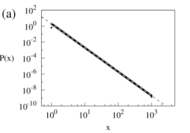
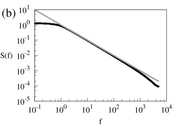
Figure 1: (a) The steady-state PDF of the signal generated by equation (1) with reflective boundaries at $x_{\mathrm{min}}$ and $x_{\mathrm{max}}$. The dashed line shows the power-law with the exponent $-3$. (b) The PSD of such a signal. The gray line shows the slope $f^{-1}$. Used parameters are $\eta=2$, $\lambda=3$, $x_{\mathrm{min}}=1$, $x_{\mathrm{max}}=1000$, and $\sigma=1$.

For $\lambda=3$ we get that $\beta=1$ and SDE (1) gives signal exhibiting $1/f$ noise. Comparison of the numerically obtained steady state PDF and the PSD with analytical expressions for SDE (1) with $\eta=2$ and $\lambda=3$ is presented in figure 1. For the numerical solution we use the Euler-Maruyama approximation, transforming the differential equations to difference equations. We use a variable time step, decreasing with the increase of $x$. As in [26, 27] we choose the time step in such a way that the coefficient before noise becomes proportional to the first power of $x$. Very similar numerical results one gets also by using the Milstein approximation [35]. We see a good agreement of the numerical results with analytical expressions. A numerical solution of the equations confirms the presence of the frequency region for which the power spectral density has $1/f^{\beta}$ dependence. The $1/f$ interval in the PSD in figure 1 is approximately between $f_{\mathrm{min}}\approx 10^{0}$ and $f_{\mathrm{max}}\approx 10^{3}$ and is much narrower than the width of the region $1\ll f\ll 10^{6}$ predicted by equation (7). The width of this region can be increased by increasing the ratio between the minimum and the maximum values of the stochastic variable $x$. In addition, the region in the power spectral density with the power-law behavior depends on the exponent $\eta$: if $\eta=1$ then this width is zero; the width increases with increasing the difference $|\eta-1|$ [43].

3 Nonlinear SDE resulting from motion in inhomogeneous medium

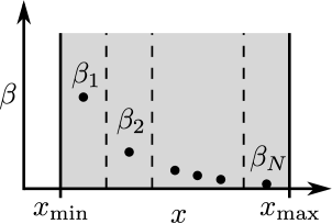
Figure 2: The schematic representation of an inhomogeneous medium. The non-equilibrium system is described as a large number $N$ of regions at local equilibrium, each region having different inverse temperature $\beta_{i}$. When the number of regions is sufficient large we can use approximation (28).

The nonlinear SDE (1) generating signals with $1/f$ spectrum in a wide range of frequencies has been used so far to describe socio-economical systems [29, 30]. The derivation of the equations has been quite abstract and physical interpretation of assumptions made in the derivation is not very clear. In this Section we present a physical model where such equation can be relevant. We expect that this derivation leads to a better understanding which systems can be described using equation (1) or equation (2).

We will consider the Brownian motion of a small macroscopic particle in an inhomogeneous medium. We assume that this medium has reached local thermodynamical equilibrium but not the global one and the temperature can be considered as a function of coordinate. Schematically such a medium is shown in figure 2. Brownian motion of small macroscopic particles in a liquid or a gas results from unbalanced bombardments due to surrounding molecules. Usually the Brownian motion is described by a Langevin equation that includes the influence of the “bath” of surrounding molecules as a time-dependent stochastic force that is commonly assumed to be a white Gaussian noise. This assumption is is valid when the correlation time of fluctuations is short, much shorter than the time scale of the macroscopic motion, and the interactions with the bath are weak. The effect of large correlation time of fluctuations will be considered in next Section. In the case of strong collisions between the particle and the surrounding environment the noise is non-Gaussian and we have so called Lévy flights [44]. Nonlinear SDEs Lévy noise and generating signals with $1/f$ spectrum are proposed in [45].

Langevin equations for one-dimensional motion of a Brownian particle are [46]

$$\frac{\rmd}{\rmd t}v(t)=-\gamma v(t)+\frac{1}{m}F(x)+\sqrt{\frac{2\gamma}{m}\frac{1}{\beta(x)}}\xi(t)\,,$$ (8)

$$\frac{\rmd}{\rmd t}x(t)=v(t)$$ (9)

Here $x$ is the coordinate and $v$ is the velocity of the Brownian particle, $m$ is the mass of the particle, $\gamma$ is the relaxation rate and $\xi(t)$ is the $\delta$-correlated white noise. In general, equations similar to (8), (9) can be used to describe a variety of systems: noisy electronic circuits, laser light intensity fluctuations [46] and others. We assume that there is temperature gradient in the medium, therefore the inverse temperature $\beta(x)$ depends on coordinate $x$. In the case when $\beta(x)\equiv\beta=\mathrm{const}$, equations (8) and (9) describe Brownian motion in the medium with constant temperature $T=k_{\mathrm{B}}^{-1}/\beta$, where $k_{\mathrm{B}}$ is Boltzmann constant.

In high friction (also called overdamped) limit [40] the relaxation rate is large, $\gamma\gg|dv/dt|$. Performing adiabatic elimination of the velocity as in [47], we obtain the equation

$$\frac{\rmd}{\rmd t}x(t)=\frac{1}{\gamma m}F(x)+\frac{1}{2\gamma m}\frac{\beta^{\prime}(x)}{\beta(x)^{2}}+\sqrt{\frac{2}{\gamma m}\frac{1}{\beta(x)}}\xi(t)\,.$$ (10)

Here $\beta^{\prime}(x)\equiv\rmd\beta(x)/\rmd x$. This SDE should be interpreted according to the Stratonovich convention. Note, that the second term in the right hand side of equation (10) arises due to position dependence of the stochastic force in equation (8) [47]. The Itô SDE corresponding to (10) is

$$\rmd x=\frac{1}{\gamma m}F(x)\rmd t+\sqrt{\frac{2}{\gamma m}\frac{1}{\beta(x)}}\rmd W_{t}\,.$$ (11)

For calculating stationary distribution of position $x$ in high friction limit we will use a Fokker-Planck equation instead of SDE (10). The Fokker-Planck equation corresponding to (10) can be written as

$$\frac{\partial}{\partial t}P(x,t)=-\frac{1}{\gamma m}\frac{\partial}{\partial x}F(x)P(x,t)+\frac{1}{\gamma m}\frac{\partial^{2}}{\partial x^{2}}\frac{P(x,t)}{\beta(x)}\,.$$ (12)

By setting the time derivative to zero we obtain an analytical expression for steady state distribution $P_{0}(x)$:

$$P_{0}(x)=C\beta(x)\exp\left(\int^{x}F(x^{\prime})\beta(x^{\prime})\rmd x^{\prime}\right)\,.$$ (13)

Let us consider the situation when the dependence of the inverse temperature on the coordinate is described by a power law,

$$\beta(x)=bx^{-\theta}\,.$$ (14)

Here $\theta$ is a power law exponent and $b$ is a constant. This is quite reasonable assumption; for example, if $\theta=1$ equation (14) represents a case where we have steady state heat transfer due to temperature difference $T_{2}-T_{1}$ between the beginning and the end of the system. We assume that there are reflective boundaries at $x_{\mathrm{min}}$ and $x_{\mathrm{max}}$ and the motion is limited to values of $x$ between $x_{\mathrm{min}}$ and $x_{\mathrm{max}}$. When $\theta=1$ then the temperatures should obey the relation $T_{2}/T_{1}=x_{\mathrm{max}}/x_{\mathrm{min}}$ and the coefficient $b$ is $b=(x_{\mathrm{max}}-x_{\mathrm{min}})/k_{\mathrm{B}}(T_{2}-T_{1})$. This case is presented in figure 2.

The external force affecting the particle $F(x)$ we express via the gradient of the potential $V(x)$:

$$F(x)=-\frac{\rmd}{\rmd x}V(x)\,.$$ (15)

We choose the subharmonic potential proportional to the temperature:

$$V(x)=\left(\frac{\nu}{\theta}-1\right)\frac{1}{\beta(x)}\,.$$ (16)

For convenience we write the coefficient of proportionality as $\nu/\theta-1$. As we will see in equation (19), the parameter $\nu$ gives the power law exponent in the steady state distribution of $x$. Taking into account equation (14) we see that the potential has the power law form with the same exponent $\theta$. The expression for the external force then is

$$F(x)=\frac{\theta}{b}x^{\theta-1}\left(1-\frac{\nu}{\theta}\right)\,.$$ (17)

Using inverse temperature (14) and force (17) the equation (10) for the particle coordinate becomes

$$\frac{\rmd}{\rmd t}x(t)=\frac{\theta}{\gamma mb}\left(\frac{1}{2}-\frac{\nu}{\theta}\right)x^{\theta-1}+x^{\frac{\theta}{2}}\sqrt{\frac{2}{\gamma m\mathrm{b}}}\xi(t)\,.$$ (18)

By using equations (13), (14) and (17) we obtain distribution of particles in high friction limit

$$P_{0}(x)=\frac{\nu-1}{x_{\mathrm{min}}^{1-\nu}-x_{\mathrm{max}}^{1-\nu}}x^{-\nu}\,.$$ (19)

Calculating distribution of particles we assumed that there are reflective boundaries at $x_{\mathrm{min}}$ and $x_{\mathrm{max}}$ and the motion is limited to values of $x$ between $x_{\mathrm{min}}$ and $x_{\mathrm{max}}$. Equation (18) has the same form as Stratonovich SDE (2).

3.1 Numerical solution

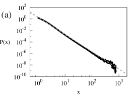
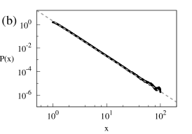
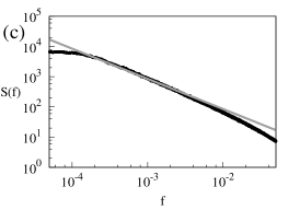
Figure 3: The steady-state PDF of the signal generated by the Langevin equations (22), (23) with reflective boundaries at $\tilde{x}_{\mathrm{min}}$ and $\tilde{x}_{\mathrm{max}}$ and the parameters: (a) $\theta=1$, $\nu=3$, $\tilde{x}_{\mathrm{min}}=1$, $\tilde{x}_{\mathrm{max}}=1000$, (b) $\theta=0$, $\nu=3$, $\tilde{x}_{\mathrm{min}}=1$, $\tilde{x}_{\mathrm{max}}=100$. The dashed line shows the power-law with the exponent $-3$. (c) The PSD of the signal corresponding to the parameters in (b) case. The gray line shows the slope $f^{-1}$.

To check the validity of the adiabatic elimination of the velocity, we solve the Langevin equations (8), (9) numerically. For numerical solution it is convenient to introduce dimensionless time $\tilde{t}$, position $\tilde{x}$ and velocity $\tilde{v}$. When the inverse temperature $\beta(x)$ and the force $F(x)$ are given by equations (14) and (17), we can use $\tilde{t}=\gamma t$ and

$$\tilde{x}=(\gamma^{2}mb)^{\frac{1}{2-\theta}}x\,,$$ (20)

$$\tilde{v}=\gamma^{-1}(\gamma^{2}mb)^{\frac{1}{2-\theta}}v\,.$$ (21)

The equations (8), (9) in the dimensionless variables have the form

$$\frac{\rmd}{\rmd\tilde{t}}\tilde{v}=-\tilde{v}+(\theta-\nu)\tilde{x}^{\theta-1}+\sqrt{2\tilde{x}^{\theta}}\xi(\tilde{t})\,,$$ (22)

$$\frac{\rmd}{\rmd\tilde{t}}\tilde{x}=\tilde{v}\,.$$ (23)

The reflective boundaries at $x_{\mathrm{min}}$ and $x_{\mathrm{max}}$ become

$$\tilde{x}_{\mathrm{min}}=(\gamma^{2}mb)^{\frac{1}{2-\theta}}x_{\mathrm{min}}\,,$$ (24)

$$\tilde{x}_{\mathrm{max}}=(\gamma^{2}mb)^{\frac{1}{2-\theta}}x_{\mathrm{max}}\,.$$ (25)

The requirement of large friction $\gamma$, necessary for the adiabatic elimination of the velocity, leads to the requirement $\tilde{x}_{\mathrm{min}},\tilde{x}_{\mathrm{max}}\gg 1$ when $\theta<2$.

Applying the Euler scheme with the step $h$ to (22), (23) yields the following equations:

$$\tilde{v}_{k+1}=\tilde{v_{k}}-\tilde{v_{k}}h+(\theta-\nu)\tilde{x}_{k}^{\theta-1}h+\sqrt{2\tilde{x}_{k}^{\theta}h}\xi_{k}\,,$$ (26)

$$\tilde{x}_{k+1}=\tilde{x}_{k}+\tilde{v}_{k}h\,.$$ (27)

Here $\xi_{k}$ are independent Gaussian random variables with zero mean and unit variance.

As an example we solve the Langevin equations (22), (23) with reflective boundaries at $\tilde{x}_{\mathrm{min}}$, $\tilde{x}_{\mathrm{max}}$ and the parameters $\nu=3$, $\theta=1$ or $\theta=0$. The value of the parameter $\theta=0$ means that the temperature is constant. The steady state PDF of the particle position $P_{0}(\tilde{x})$ and the power spectral density $S(\tilde{f})$ are presented in figure 3. In figure 3a we see a good agreement with the distribution of particles in high friction limit (19). This confirms the validity of the adiabatic elimination of the velocity. Figure 3c confirms the presence of the frequency region with $1/f$ behavior of the power spectral density, the $1/f$ interval in the PSD is approximately between $\tilde{f}_{\mathrm{min}}\approx 10^{-4}$ and $\tilde{f}_{\mathrm{max}}\approx 10^{-2}$. The width of this interval can be increased by increasing the ratio $\tilde{x}_{\mathrm{max}}/\tilde{x}_{\mathrm{min}}$. The width of $1/f^{\beta}$ region in the PSD also increases with increasing of $|\theta/2-1|$.

Not only coordinate fluctuations yield power law PSD. The Langevin equation with postion dependent temperature (14) and external force (17) can also lead to the power law PSD of the absolute velocity fluctuations.

3.2 Superstatistics and velocity fluctuations

In the motion of the particle there are two time scales: the scale in which the particle is able to reach a local equilibrium and the scale at which the fluctuating temperature changes. We assume that temperature fluctuations are slow, that is, the time scale at which observable change of temperature happens is much larger that relaxation time of the particle $1/\gamma$. This assumption empowers us to derive simpler equations for particle velocity and apply the superstaticlical approach [48, 49, 50, 51, 52] to obtain statistical properties of particle velocity fluctuations. The superstatistical framework has been successfully applied to a wide range of problems, such as interactions between hadrons from cosmic rays [53], fluid turbulence [54, 55, 56, 57], granular material [58] and electronics [59]. In the long-term the nonequilibrium system is described by the superposition of different local dynamics at different time intervals. Superstatistics is a description of the complex system under consideration by a superposition of two statistics, one corresponding to ordinary statistical mechanics (Langevin equation) and the other one corresponding to a slowly varying parameter, in this case the inverse temperature $\beta(x)$. In the superstatistical approach the distribution of the velocity of the particle is

$$P(v)=\sum_{i=1}^{N}f(\beta_{i})P(v|\beta_{i})\approx\int_{\beta_{\mathrm{min}}}^{\beta_{\mathrm{max}}}f(\beta)P(v|\beta)\rmd\beta\,,$$ (28)

where $P(v|\beta)$ is a local velocity distribution for the particle near the position $x$ when the temperature can be assumed to be constant and equal to $\beta(x)=\beta$. For the Langevin equation in the form of equation (8) the local velocity distribution is

$$P(v|\beta)=\mathrm{\sqrt{\frac{m\beta}{2\pi}}}\exp\left(-\frac{1}{2}m\beta v^{2}\right)\,.$$ (29)

The function $f(\beta)$ is the distribution of the inverse temperature. The distribution of the inverse temperature $f(\beta)$ can be found from the stationary distribution $P_{0}(x)$ of coordinate $x$ by using the relation [60]

$$f(\beta)=\left(\frac{\rmd\beta}{\rmd x}\right)^{-1}P_{0}(x(\beta)).$$ (30)

The parameters

$$\beta_{\mathrm{max}}=bx_{\mathrm{min}}^{-\theta}\,,\qquad\beta_{\mathrm{min}}=\mathrm{b}x_{\mathrm{max}}^{-\theta}$$ (31)

are maximal and minimal inverse temperatures. From equations (30), (19) and (14) we obtain the distribution of inverse temperature

$$f(\beta)=\frac{\nu-1}{\theta\left(\beta_{\mathrm{max}}^{\frac{\nu-1}{\theta}}-\beta_{\mathrm{min}}^{\frac{\nu-1}{\theta}}\right)}\beta^{\frac{\nu-1}{\theta}-1}\,.$$ (32)

Now we will describe fluctuations of particle velocity. For this purpose we introduce the local average of absolute value of the velocity

$$\bar{v}\equiv\int\limits_{-\infty}^{\infty}|v|P(v|\beta)\rmd v\,.$$ (33)

Keeping the assumption that local distribution of the velocity remains Gaussian (29), we have

$$\bar{v}=\sqrt{\frac{2}{\pi m\beta(x)}}=x^{\frac{\theta}{2}}\sqrt{\frac{2}{\pi m\mathrm{b}}}\,.$$ (34)

By using equation (34) and changing the variable from $x$ to $\bar{v}$ in Stratonovich SDE (18) [40], we obtain an SDE for the average velocity

$$\frac{\rmd}{\rmd t}\bar{v}=\frac{1}{2}\sigma^{2}(\eta-\lambda)\bar{v}^{2\eta-1}+\sigma\bar{v}^{\eta}\xi(t)\,.$$ (35)

Here we introduced the new parameters

$$\eta=2\left(1-\frac{1}{\theta}\right)\,,\qquad\lambda=\frac{2}{\theta}(\nu-1)+1$$ (36)

and noise intensity

$$\sigma=\theta\sqrt{\frac{\pi}{4\gamma}}\left(\frac{2}{\pi mb}\right)^{\frac{1}{\theta}}\,.$$ (37)

The equation (35) for the average absolute velocity is identical to SDE (2) generating power-law distributed signals with $1/f^{\alpha}$ spectrum. The multiplicity of noise $\eta$ in equation (35) depends only on power-law exponent $\theta$, whereas the exponent $\lambda$ of the power law part of distribution of $\bar{v}$ depends on both parameters $\theta$ and $\nu$. According to equation (6) we have $1/f$ noise when $\lambda=3$ or $\nu=\theta+1$. One can expect that fast velocity fluctuations do not influence the spectrum at small frequencies and $1/f$ noise is visible not only in the spectrum of the local average $\bar{v}$ but also in the spectrum of the absolute value of the velocity $|v|$. Numerical calculation confirms this expectation.

From equations (28) and (32) we get

$$P(v)=\frac{\lambda-1}{2\sqrt{\pi}\left(\beta_{\mathrm{max}}^{\frac{\lambda-1}{2}}-\beta_{\mathrm{min}}^{\frac{\lambda-1}{2}}\right)}\left(\frac{2}{m}\right)^{\frac{\lambda-1}{2}}|v|^{-\lambda}\left[\Gamma\left(\frac{\lambda}{2},\frac{1}{2}mv^{2}\beta_{\mathrm{min}}\right)-\Gamma\left(\frac{\lambda}{2},\frac{1}{2}mv^{2}\beta_{\mathrm{max}}\right)\right]$$ (38)

Here $\Gamma(a,z)=\int_{z}^{\infty}t^{a-1}\rme^{-t}\rmd t$ is the incomplete gamma function. When $\frac{1}{2}mv^{2}\beta_{\mathrm{min}}\ll 1$ and $\frac{1}{2}mv^{2}\beta_{\mathrm{max}}\gg 1$ then from equation (38) it follows that the distribution of velocities has a power law form $P(v)\sim|v|^{-\lambda}$.

Thus we obtain $1/f$ noise in the fluctuations of the absolute value of the velocity when the velocity distribution has a power-law part $P(v)\sim v^{-3}$ and temperature distribution is flat, $f(\beta)=\mathrm{const}$. When $\theta=1$ we have a simple system exhibiting $1/f$ fluctuations: the system consists of a Brownian particle affected by a linear potential $V(x)$ and moving in the medium where steady state heat transfer is present due to the difference of temperatures at the ends of the medium.

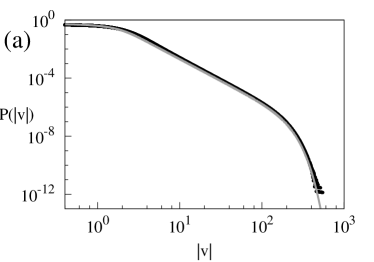
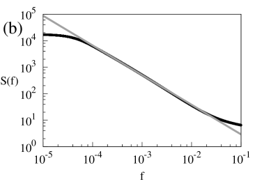
Figure 4: (a) The steady-state PDF of the absolute velocity obtained by numerically solving the Langevin equations (22), (23) with reflective boundaries at $\tilde{x}_{\mathrm{min}}$ and $\tilde{x}_{\mathrm{max}}$. The gray line shows the PDF from equation (38) multiplied by 2. (b) The PSD of the absolute velocity fluctuations. The gray line shows the slope $f^{-1.1}$. The parameters used are: $\theta=1$, $\nu=2$, $\tilde{x}_{\mathrm{min}}=1$, $\tilde{x}_{\mathrm{max}}=10^{4}$.

As an example we solve the Langevin equations (22), (23) with reflective boundaries at $\tilde{x}_{\mathrm{min}}$, $\tilde{x}_{\mathrm{max}}$ and the parameters $\nu=2$, $\theta=1$. The steady state PDF of the absolute velocity $P(|\tilde{v}|)$ and the power spectral density $S(\tilde{f})$ of the absolute velocity fluctuations are presented in figure 4. The steady state PDF $P(|v|)$ is twice as large as the PDF given by equation (38) because both positive and negative velocities with the same absolute value occur with equal probabilities. The PDF of the dimensionless velocity $\tilde{v}$ can be obtained by setting $m=1$, $b=1$. In figure 4a we see a good agreement with the analytical expression for the steady state PDF. Figure 4b confirms the presence of the frequency region with the power law behavior of the PSD. The power law region in the PSD is approximately between $\tilde{f}_{\mathrm{min}}\approx 10^{-4}$ and $\tilde{f}_{\mathrm{max}}\approx 10^{-2}$. However, there is a slight difference between the power law exponent equal to $1$ predicted by analytical expressions and the numerically obtained power law exponent $1.1$. This disagreement arises because the analytical prediction of the power law exponent in the spectrum is only approximate.

4 Stochastic differential equations with colored noise

A system subjected to the colored noise is described by the Langevin equation with a time-dependent stochastic force that includes the influence of the “bath” of surrounding molecules:

$$\frac{\rmd x}{\rmd t}=f(x)+g(x)\varepsilon(t)\,.$$ (39)

It is a well known result that if we approximate white noise by a smooth, colored process, then at the limit as the correlation time of the approximation tends to zero, the smoothed stochastic integral converges to the Stratonovich stochastic integral [61]. We assume that the stochastic force in equation (39) is a Gaussian noise having correlation time comparable with time scale of the macroscopic motion and that $\varepsilon(t)$ is Markovian process. In such a case the noise $\varepsilon$ satisfies Ornstein-Uhlenbeck process with exponential correlation function [62]. Thus we describe the system perturbed by a colored noise as two-dimensional Markovian flow:

$$\frac{\rmd x}{\rmd t}=f(x)+g(x)\varepsilon\,,$$ (40)

$$\frac{\rmd\varepsilon}{\rmd t}=-\frac{1}{\tau}\varepsilon+\frac{\sqrt{2D}}{\tau}\xi(t)\,.$$ (41)

Here $\xi(t)$ is the white noise, $\langle\xi(t)\xi(s)\rangle=\delta(t-s)$, the parameter $\tau$ is the correlation time of the colored noise and $D$ is the noise intensity. The autocorrelation function of the colored noise is

$$\langle\varepsilon(t)\varepsilon(s)\rangle=\frac{D}{\tau}\exp\left(-\frac{|t-s|}{\tau}\right)\,.$$ (42)

It is possible to write two dimensional Fokker-Planck equation for equations (40), (41) and obtain two dimensional $P(x,\varepsilon)$ density as its solution. However, usually it is enough to know the distribution $P(x)$ of the signal $x$, which can be formally obtained by averaging $P(x,\varepsilon)$ over the noise $\varepsilon$. It is problematic even get approximate analytical solutions for $P(x,\epsilon)$ [63]. More convenient way is to get $P(x)$ from an approximate Fokker-Planck equation just for one variable. Such equation can be obtained by using the unified colored noise approximation [64], which is a form of adiabatic approximation. To make this approximation we eliminate the variable $\varepsilon$ and get the equation

$$\frac{\rmd^{2}x}{\rmd t^{2}}=\frac{g^{\prime}(x)}{g(x)}\left(\frac{\rmd x}{\rmd t}\right)^{2}-\left(\frac{1}{\tau}-f^{\prime}(x)+f(x)\frac{g^{\prime}(x)}{g(x)}\right)\frac{\rmd x}{\rmd t}+\frac{1}{\tau}f(x)+\frac{\sqrt{2D}}{\tau}g(x)\xi(t)\,.$$ (43)

We assume that the variable $x$ changes slowly and drop small terms containing $\rmd^{2}x/\rmd t^{2}$ and $(\rmd x/\rmd t)^{2}$, obtaining the approximate equation

$$\frac{\rmd x}{\rmd t}=\frac{f(x)}{1-\tau\left(f^{\prime}(x)-f(x)\frac{g^{\prime}(x)}{g(x)}\right)}+\frac{\sqrt{2D}g(x)}{1-\tau\left(f^{\prime}(x)-f(x)\frac{g^{\prime}(x)}{g(x)}\right)}\xi(t)\,.$$ (44)

This equation should be interpreted in the Stratonovich sense. In more general case, when we cannot neglect inertia and drop the second derivative $d^{2}x/dt^{2}$, the question whether the equation obtained using adiabatic approximation should be interpreted in Itô or Stratonovich sense still remains an open question, so called Itô-Stratonovich problem [65]. However, at least for specific systems in white noise limit, it can be determined which interpretation is correct. For example, it has been shown for a simplified model of the preferential concentration of inertial particles in a turbulent velocity field [66], that the equation obtained using adiabatic elimination in white noise limit became the Stratonovich equation [67]. The Stratonovich interpretation should be used if the correlation time of the noise is much larger than the relaxation rate of the system. In an opposite case the equation should be interpreted in Itô sense. If relaxation rates are of the similar magnitude as the correlation time, we get an equation with noise induced drift that is different from Stratonovich drift.

The Fokker-Planck equation corresponding to the Stratonovich equation $\rmd x/\rmd t=f_{\mathrm{c}}(x)+g_{\mathrm{c}}(x)\xi(t)$ is [40]

$$\frac{\partial}{\partial t}P(x,t)=-\frac{\partial}{\partial x}f_{c}(x)P(x,t)+\frac{1}{2}\frac{\partial}{\partial x}g_{c}(x)\frac{\partial}{\partial x}g_{c}(x)P(x,t)\,.$$ (45)

The applicability of equations (44) and (45) has limitation due to neglect of higher order derivatives in equation (43). These equations describe the dynamics correctly [64] for times $t$ obeying

$$t\gg\frac{\tau}{1-\tau\left(f^{\prime}(x)-f(x)\frac{g^{\prime}(x)}{g(x)}\right)}$$ (46)

and in the space regions obeying

$$\frac{\sqrt{2D\tau}g(x)}{1-\tau\left(f^{\prime}(x)-f(x)\frac{g^{\prime}(x)}{g(x)}\right)}\left|\frac{f^{\prime}(x)}{f(x)}\right|\ll 1\,.$$ (47)

5 Influence of colored noise on the stochastic differential equation generating signals with $1/f$ spectrum

If the nonlinear SDE generating signals with $1/f$ spectrum is a result of a Brownian motion in an inhomogeneous medium then the finite correlation time of the “bath” can become important. In this section we use the results presented in section 4 to investigate the influence of the colored noise. Instead of white noise we add colored noise $\varepsilon(t)$ to the Stratonovich equation (2) obtaining the equations

$$\frac{\rmd x}{\rmd t}=\frac{1}{2}\sigma^{2}(\eta-\lambda)x^{2\eta-1}+\sigma x^{\eta}\varepsilon(t)\,,$$ (48)

$$\frac{\rmd\varepsilon}{\rmd t}=-\frac{1}{\tau}\varepsilon+\frac{1}{\tau}\xi(t)\,.$$ (49)

After unified colored noise approximation (44) we get

$$\frac{\rmd x}{\rmd t}=\frac{\frac{1}{2}\sigma^{2}(\eta-\lambda)x^{2\eta-1}}{1-\frac{1}{2}\tau\sigma^{2}(\eta-1)(\eta-\lambda)x^{2(\eta-1)}}+\frac{\sigma x^{\eta}}{1-\frac{1}{2}\tau\sigma^{2}(\eta-1)(\eta-\lambda)x^{2(\eta-1)}}\xi(t)\,.$$ (50)

If $\tau$ is large then equation (50) has a simpler form

$$\frac{\rmd x}{\rmd t}=-\frac{x}{\tau(\eta-1)}+\frac{2x^{2-\eta}}{\tau\sigma(\eta-1)(\lambda-\eta)}\xi(t)\,.$$ (51)

Equation (50) should be interpreted in the Stratonovich sense. Converting to Itô interpretation [40] we have

$$\rmd x=\frac{1}{2}\frac{\sigma^{2}x^{2\eta-1}}{\gamma(x)}\left[\eta-\lambda+\frac{2-\eta}{\gamma(x)}+\frac{2(\eta-1)}{\gamma(x)^{2}}\right]\rmd t+\frac{\sigma x^{\eta}}{\gamma(x)}\rmd W_{t}\,,$$ (52)

where

$$\gamma(x)\equiv 1-\frac{1}{2}\tau\sigma^{2}(\eta-1)(\eta-\lambda)x^{2(\eta-1)}$$ (53)

According to equation (47), approximation (50) is valid when

$$\frac{\sqrt{\tau}\sigma|2\eta-1|x^{\eta-1}}{1-\frac{1}{2}\tau\sigma^{2}(\eta-1)(\eta-\lambda)x^{2(\eta-1)}}\ll 1$$ (54)

Steady state PDF corresponding to equation (50) is

$$P_{0}(x)\sim x^{-\lambda}\left(1-\frac{1}{2}\tau\sigma^{2}(\eta-1)(\eta-\lambda)x^{2(\eta-1)}\right)\exp\left[-\frac{1}{4}\tau\sigma^{2}(\eta-\lambda)^{2}x^{2(\eta-1)}\right]$$ (55)

We see that the colored noise introduces an exponential cut-off in the steady state PDF $P_{0}(x)$ and naturally limits the range of diffusion of the stochastic variable $x$. The exponential cut-off is at large values of $x$ when $\eta>1$ and at small values of $x$ when $\eta<1$.

Comparing equation (50) with (2) we see that the influence of the finite correlation time $\tau$ of the noise can be neglected when

$$\frac{1}{2}\tau\sigma^{2}|\eta-1||\eta-\lambda|x^{2(\eta-1)}\ll 1\,.$$ (56)

Let us consider the case $\eta>1$. Then according to equation (56), the influence of the finite correlation time $\tau$ of the noise can be neglected when $x\ll x_{\tau}$, where

$$x_{\tau}\equiv\left[\frac{2}{\tau\sigma^{2}(\eta-1)|\eta-\lambda|}\right]^{\frac{1}{2(\eta-1)}}$$ (57)

If the diffusion is restricted to the region $x_{\mathrm{min}}<x<x_{\mathrm{max}}$ then the spectrum has a power-law part in the frequency range given by (7). If $x_{\tau}>x_{\mathrm{max}}$ we expect no change in the power-law part of the spectrum. If $x_{\tau}<x_{\mathrm{max}}$ then, replacing the maximum value of $x$ by $x_{\tau}$ we get that the replacement of the white noise by the colored noise leaves the power-law part of the spectrum in the frequency range

$$\sigma^{2}x_{\mathrm{min}}^{2(\eta-1)}\ll 2\pi f\ll\frac{2}{\tau(\eta-1)|\eta-\lambda|}\,.$$ (58)

If $\eta<1$ then the influence of the finite correlation time $\tau$ of the noise can be neglected when $x\gg x_{\tau}$, where $x_{\tau}$ is given by (57). When the diffusion is restricted to the region $x_{\mathrm{min}}<x<x_{\mathrm{max}}$, we expect no change in the power-law part of the spectrum when $x_{\tau}<x_{\mathrm{min}}$. If $x_{\tau}>x_{\mathrm{min}}$ then replacing the minimum value of $x$ by $x_{\tau}$ in equation (7) we can estimate that the power-law part of the spectrum should be in the frequency range

$$\sigma^{2}x_{\mathrm{max}}^{-2(1-\eta)}\ll 2\pi f\ll\frac{2}{\tau(1-\eta)|\eta-\lambda|}\,.$$ (59)

Thus the introduction of the colored noise into equation (2) can narrow the range of frequencies where the PSD behaves as $1/f^{\beta}$ by decreasing the upper limiting frequency.

5.1 Numerical solution

Figure 5: (a) Typical signal generated by equations (48), (49) with $\tau=0.01$. (b) Typical signal generated by equation (2) corresponding to $\tau=0$ (white noise). We used reflective boundaries at $x_{\mathrm{min}}=1$ and $x_{\mathrm{max}}=1000$. Other parameters of equations are $\eta=2$, $\lambda=3$, and $\sigma=1$.

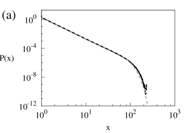
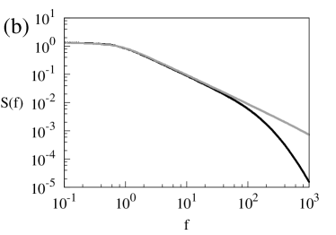
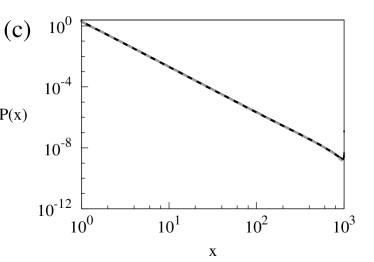
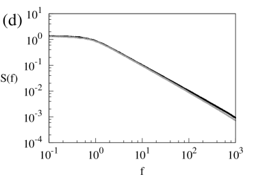
Figure 6: (a,c) The steady-state PDF of the signal generated by equations (65))–(67) with reflective boundaries at $x_{\mathrm{min}}$ and $x_{\mathrm{max}}$. The dashed line shows analytical approximation (55). (b,d) The PSD of such a signal. The gray line shows the PSD of the signal generated by equation (2). The correlation time is (a,b) $\tau=10^{-3}$, (c,d) $\tau=10^{-5}$. Other parameters are $\eta=2$, $\lambda=3$, $x_{\mathrm{min}}=1$, $x_{\mathrm{max}}=1000$, and $\sigma=1$.

To check the validity of the approximations we performed numerical solution of equations (48), (49). For numerical solution we used the Euler scheme [68, 69]. Applying the Euler scheme with the step $h$ to (48), (49) yields the following equations:

$$x_{k+1}=x_{k}+\left(\frac{1}{2}\sigma^{2}(\eta-\lambda)x_{k}^{2\eta-1}+\sigma x_{k}^{\eta}z_{k}\right)h\,,$$ (60)

$$z_{k+1}=z_{k}-\frac{1}{\tau}z_{k}h+\frac{1}{\tau}\sqrt{h}\xi_{k}\,.$$ (61)

Here $\xi_{k}$ are independent Gaussian random variables with zero mean and unit variance. For $\eta<1$ and for negative $\eta$ it is convenient to use the Euler scheme with a constant time step $h$. However, in the case of $\eta>1$ at large values of $x$ the coefficient in equation (60) becomes large and thus requires a very small time step. A more effective solution is to use a variable time step, decreasing with the increase of $x$, as has been done in Refs. [26, 27]. Variable time step $h_{k}=\kappa\tau/(\sigma x_{k}^{\eta})$ leads to the equations

$$x_{k+1}=x_{k}+\kappa\tau\left(\frac{1}{2}\sigma(\eta-\lambda)x_{k}^{\eta-1}+z_{k}\right)\,,$$ (62)

$$z_{k+1}=z_{k}-\frac{\kappa}{\sigma x_{k}^{\eta}}z_{k}+\sqrt{\frac{\kappa}{\sigma\tau x_{k}^{\eta}}}\xi_{k}\,,$$ (63)

$$t_{k+1}=t_{k}+\frac{\kappa\tau}{\sigma x_{k}^{\eta}}\,.$$ (64)

Here $\kappa\ll 1$ is a small parameter.

As an example, we solve equations (48), (49) with the parameters $\eta=2$, $\lambda=3$, $\sigma=1$ and reflective boundaries at $x_{\mathrm{min}}=1$, $x_{\mathrm{max}}=1000$. From equations (62)–(64) we get

$$x_{k+1}=x_{k}+\kappa\tau\left(z_{k}-\frac{1}{2}x_{k}\right)\,,$$ (65)

$$z_{k+1}=z_{k}-\frac{\kappa}{x_{k}^{2}}z_{k}+\frac{1}{x_{k}}\sqrt{\frac{\kappa}{\tau}}\xi_{k}\,,$$ (66)

$$t_{k+1}=t_{k}+\frac{\kappa\tau}{x_{k}^{2}}\,.$$ (67)

The generated signal is shown in figure 5. We see that the finite correlation time $\tau$ of the noise leads to a smoother signal compared to the equation with $\tau=0$. The steady state PDF $P_{0}(x)$ and the power spectral density $S(f)$ for two different values of $\tau$ are presented in figure 6. From figure 6a we see that the unified colored noise approximation correctly predicts the exponential cut-off in the steady state PDF at large values of $x$, although the actual position of the cut-off slightly differs from the cut-off predicted by equation (55). As figure 6b shows, the presence of the finite correlation time $\tau$ makes the power-law part in the spectrum narrower. The upper limiting frequency of the power-law region grows with decreasing of $\tau$, as is qualitatively predicted by equation (58). The steady state PDF and the PSD of the generated signal corresponding to much smaller value of the correlation time $\tau$ are shown in figure 6b,d. For this value of $\tau$ the exponential cut-off due to finite correlation time is larger than the upper boundary $x_{\mathrm{max}}$, thus we see almost no differences from the case of uncorrelated noise, $\tau=0$.

6 Discussion

The nonlinear SDE (1) generating signals with $1/f$ spectrum in a wide range of frequencies has been used so far to describe socio-economical systems [29, 30]. The derivation of the equations has been quite abstract and physical interpretation of assumptions made in the derivation is not very clear. In this paper we propose a physical model where such equations can be relevant. This model is described by Stratonovich (2) instead of Itô (1) SDE and provides insights which physical systems can be described by such nonlinear SDEs.

We have shown that nonlinear SDEs generating power-law distributed precesses with $1/f^{\beta}$ spectrum can result from diffusive particle motion in inhomogeneous medium. The SDE (35) for velocity fluctuations or SDE (18) for particle coordinate are simplified versions of Langevin equations (8), (9) for one-dimensional motion of a Brownian particle. We neglected viscosity dependence on temperature and inertia of particle. In general, equations similar to these can be used to describe a variety of systems: noisy electronic circuits, laser light intensity fluctuations [46] and others. We assumed that the inverse temperature $\beta(x)$ depends on coordinate $x$ and this dependence is of a power law form. Such a description is valid for a medium that has reached local thermodynamical equilibrium but not the global one, and the temperature can be considered as a function of coordinate. The power law dependence of the inverse temperature $\beta(x)$ on the stochastic variable $x$ can be caused by non-homogeneity of a bath. This non-homogeneity can arise from a complex scale free structure of the bath as is in the case of porous media [70] or from the bath not being in an equilibrium.

In high friction limit, if the particle is affected by a subharmonic potential proportional to the local temperature, the motion of the particle can be described by the equation similar to equation (2). For example, we can consider a Brownian particle affected by a linear potential $V(x)$ and moving in the medium where steady state heat transfer is present due to the difference of temperatures at the ends of the medium. From the properties of equation (2), presented in section 2, it follows that the spectrum of the fluctuations of the particle position $x(t)$ in such a system can have a frequency region where the spectrum has a power-law behavior. The width of this frequency region increases with the increase of the length of the medium in which the particle moves. Equation (2) can also describe the fluctuations of the local average of the absolute value of the velocity, if temperature fluctuations are slow and the superstatistical approach can be used. We obtain $1/f$ noise in the fluctuations of the absolute value of the velocity when the velocity distribution has a power-law part $P(v)\sim v^{-3}$ and temperature distribution is flat, $f(\beta)=\mathrm{const}$.

The correlation of collisions between the Brownian particle and the surrounding molecules can lead to the situation where the finite correlation time becomes important, thus we have investigated the effect of colored noise in our model. Using the unified colored noise approximation we get that the finite correlation time leads to the additional restriction of the diffusion. Existence of colored noise leads to an exponential cut-off of the PDF of particle positions either from large values when $\eta>1$, or from small values when $\eta<1$. Such a restriction of the diffusion is a result of the multiplicative colored noise in equation (48). Narrower power law part in the PDF of the particle positions results in the narrower range of frequencies where the spectrum has $1/f^{\beta}$ behavior. When $\eta>1$ , the end of the power-law part of the spectrum at large frequencies is inversely proportional to the correlation time $\tau$ of the noise. However, for sufficiently small correlation time, when the restriction of the diffusion due to colored noise is larger than the upper boundary $x_{\mathrm{max}}$ of the medium, the effects of the colored noise are negligible (see figure 6) and the properties of the signal do not differ significantly from the white noise case.

References

References

- [1] Franosch T, Grimm M, Belushkin M, Mor F M, Foffi G, Forró L and Jeney S 2011 Nature 478 85
- [2] Landau L and Lifshits E 1987 Fluid Mechanics, Course of Theoretical Physics Vol 6 (Butterworth-Heinemann)
- [3] Zhou X 2009 Phys. Rev. A 80 023818
- [4] Kim S, Park S H and Ryu C S 1998 Phys. Rev. E 58 7994
- [5] Lande R 1993 Am. Nat. 142 911
- [6] Kamenev A, Meerson B and Shklovskii B 2008 Phys. Rev. Lett. 101 268103
- [7] Wang Y, Lai Y, and Zheng Z 2009 Phys. Rev. E 79 056210
- [8] Gammaitoni L, Hänggi and Marchesoni F 1998 Rev. Mod. Phys. 70 223
- [9] Nozaki D, Mar D J, Grigg P and Collins J J 1999 Phys. Rev. Lett. 82 2402
- [10] Ward L M and Greenwood P E 2007 Scholarpedia 2 1537
- [11] Weissman M B 1988 Rev. Mod. Phys. 60 537
- [12] Barabasi A L and Albert R 1999 Science 286 509
- [13] Gisiger T 2001 Biol. Rev. 76 161
- [14] Wagenmakers E J, Farrell S and Ratcliff R 2004 Psychonomic Bull. Rev. 11 579
- [15] Szabo G and Fath G 2007 Phys. Rep. 446 97
- [16] Castellano C, Fortunato S and Loreto V 2009 Rev. Mod. Phys. 81 591
- [17] Balandin A A 2013 Nature Nanotechnology 8 549
- [18] Kogan S 2008 Electronic Noise and Fluctuations in Solids (Cambrige Univ. Press)
- [19] Li M and Zhao W 2012 Math. Probl. Egin. 2012 23
- [20] Orlyanchik V, Weissman M B, Torija M A, Sharma M and Leighton C 2008 Phys. Rev. B 78 094430
- [21] Melkonyan S V 2010 Physica B 405 379
- [22] Marinari E, Parisi G, Ruelle D and Windey P 1983 Phys. Rev. Lett. 50 1223
- [23] Kaulakys B and Meškauskas T 1998 Phys. Rev. E 58 7013
- [24] Kaulakys B 1999 Phys. Lett. A 257 37
- [25] Kaulakys B, Gontis V and Alaburda M 2005 Phys. Rev. E 71 051105
- [26] Kaulakys B and Ruseckas J 2004 Phys. Rev. E 70 020101(R)
- [27] Kaulakys B, Ruseckas J, Gontis V and Alaburda M 2006 Physica A 365 217
- [28] Ruseckas J, Kaulakys B and Gontis V 2011 EPL 96 60007
- [29] Gontis V, Ruseckas J and Kononovicius A 2010 Physica A 389 100–106
- [30] Mathiesen J, Angheluta L, Ahlgren P T H and Jensen M H 2013 PNAS 110 17259
- [31] Hottovy S, Volpe G and Wehr J 2012 EPL 99 60002
- [32] Piazza R and Parola A 2008 J. Phys.: Condens. Matter 20 153102
- [33] Piazza R 2008 Soft Matter 4 1740
- [34] Ghosh A W and Khare S V 2000 Phys. Rev. Lett. 84 5243
- [35] Kaulakys B and Alaburda M 2009 J. Stat. Mech. 2009 P02051
- [36] Kononovicius A and Gontis V 2012 Physica A 391 1309
- [37] Jeanblanc M, Yor M and Chesney M 2009 Mathematical Methods for Financial Markets (London: Springer)
- [38] Turelli M 1977 Theor. Pop. Biol. 12 140–178
- [39] Smythe J, Moss F and McClintock P V E 1983 Phys. Rev. Lett. 51 1062
- [40] Gardiner C W 2004 Handbook of Stochastic Methods for Physics, Chemistry and the Natural Sciences (Berlin: Springer-Verlag)
- [41] Pesce G, McDaniel A, Hottovy S, Wehr J and Volpe G 2013 Nat. Commun. 4 2733
- [42] Ruseckas J and Kaulakys B 2014 J. Stat. Mech. 2014 P06005
- [43] Ruseckas J and Kaulakys B 2010 Phys. Rev. E 81 031105
- [44] Weron A, Burnecki K, Mercik S and Weron K 2005 Phys. Rev. E 71 016113
- [45] Kazakevičius R and Ruseckas J 2014 Physica A 411 95
- [46] Risken H 1989 The Fokker-Planck equation, Methods of Solution and Applications (Springer-Verlag)
- [47] Sancho J M, San Miguel M and Dürr D 1982 J. Stat. Phys. 291
- [48] Beck C and Cohen E G D 2003 Physica A 322 267–275
- [49] Tsallis C and Souza A M C 2003 Phys. Rev. E 67 026106
- [50] Abe S, Beck C and Cohen E G D 2007 Phys. Rev. E 76 031102
- [51] Hahn M G, Jiang X and Umarov S 2010 J. Phys. A: Math. Theor. 43 165208
- [52] Beck C 2011 Philos. Trans. R. Soc. A 369 453
- [53] Wilk G and Włodarczyk Z 2000 Phys. Rev. Lett. 84 2770
- [54] Beck C 2001 Phys. Rev. Lett. 87 180601
- [55] Beck C, Cohen E G D and Swinney H L 2005 Phys. Rev. E 72 056133
- [56] Beck C, Cohen E G D and Rizzo S 2005 Europhys. News 36 189
- [57] Beck C 2007 Phys. Rev. Lett. 98 064502
- [58] Beck C 2006 Physica A 365 96
- [59] Sattin F and Salasnich L 2002 Phys. Rev. E 65 035106(R)
- [60] Van der Straeten E and Beck C 2011 Chinese. Sci. Bull. 56 3633
- [61] Wong E and Zakai M 1965 Ann. Math. Stat. 36 1560
- [62] Doob J L 1944 Ann. Math. Stat. 15 229
- [63] Hänggi P and Jung P 1995 Adv. Chem. Phys. 89 239
- [64] Jung P and Hänggi P 1987 Phys. Rev. A 35 4464
- [65] Graham R and Schenzle A 1982 Phys. Rev. A 26 1676
- [66] Sigurgeirsson H and Stuart A M 2002 Phys. Fluids 14 4352
- [67] Kupferman R, Pavliotis G A and Stuart A M 2004 Phys. Rev. E 70 036120
- [68] Fox R F, Gatland I R, Roy R and Vemuri G 1988 Phys. Rev. A 38 5938
- [69] Milshtein G N and Tret’yakov M V 1994 J. Stat. Phys. 77 691
- [70] Kulasiri D 2002 Stochastic Dynamics. Modeling Solute Transport in Porous Media (North-Holland)