Chemical Abundances and Dust in the Halo Planetary Nebula K648 in M15:
Its Origin and Evolution based on an Analysis of Multiwavelength Data

Abstract

We report an investigation of the extremely metal-poor and C-rich planetary nebula (PN) K648 in the globular cluster M15 using the UV to far-IR data obtained using the Subaru, HST, FUSE, Spitzer, and Herschel. We determined the nebular abundances of ten elements. The enhancement of F ([F/H]=+0.96) is comparable to that of the halo PN BoBn1. The central stellar abundances of seven elements are determined. The stellar C/O ratio is similar to the nebular C/O ratios from recombination line and from collisionally excited line (CEL) within error, and the stellar Ne/O ratio is also close to the nebular CEL Ne/O ratio. We found evidence of carbonaceous dust grains and molecules including Class B 6-9 $\mu$m and 11.3 $\mu$m polycyclic aromatic hydrocarbons and the broad 11 $\mu$m feature. The profiles of these bands are similar to those of the C-rich halo PNe H4-1 and BoBn1. Based on the theoretical model, we determined the physical conditions of the gas and dust and their masses, i.e., 0.048 $M_{\odot}$ and 4.95$\times$10^-7 $M_{\odot}$, respectively. The observed chemical abundances and gas mass are in good agreement with an asymptotic giant branch nucleosynthesis model prediction for stars with an initial 1.25 $M_{\odot}$ plus a 2.0$\times$10^-3 $M_{\odot}$ partial mixing zone (PMZ) and stars with an initial mass of 1.5 $M_{\odot}$ without a PMZ. The core-mass of the central star is approximately 0.61-0.63 $M_{\odot}$. K648 is therefore likely to have evolved from a progenitor that experienced coalescence or tidal disruption during the early stages of evolution, and became a $\sim$1.25-1.5 $M_{\odot}$ blue straggler.

1. Introduction

Planetary nebulae (PNe) represent a stage in the evolution of initial $\sim$1-8 $M_{\odot}$ stars. At the end of their evolution, such stars evolve into asymptotic giant branch (AGB) stars, then PNe, and finally white dwarves (WD). During this process of evolution, these stars eject a large fraction of their mass into the interstellar medium. The history of the progenitors is imprinted in the central star of the PN (CSPN) and the ejected gas. An investigation of the CSPN and the ejected material provides useful information to increase our understanding of stellar evolution, as well as the chemical evolution of galaxies, i.e., how much of the mass of the star becomes a PN, which and how much of the elements are synthesized in the inner core of the progenitor, and how galaxies become chemically rich. The ejected gas in the PNe consists of both processed and unprocessed matter: primordial sources of proto-star cluster clouds or intracluster medium, pollution sources from highly evolved stars AGB and supernovae (SNe), and the result of stellar evolution processes (nucleosynthesized elements, molecules, and dust). Our understanding of the evolution of low-mass stars formed in the early Galaxy, as well as the chemical evolution of the Galaxy, can be enhanced by studying metal-poor PNe located in the Galactic halo.

Fourteen Galactic halo PNe have been identified since the discovery of K648 in M15 (e.g., Howard et al., 1997; Jacoby et al., 1997; Péquignot & Tsamis, 2005; Pereira & Miranda, 2007). Recently, the number of detections has steadily increased due to the Sloan Digital Sky Survey (SDSS) (Yuan & Liu, 2013). Five PNe are located in the globular clusters (GCs) M15 (K648), M22 (GJJC1 and M2-29), Pal6 (JaFu1), and NGC6441 (JaFu2), and others are located in the Galactic halo field. The classification of PNe based on chemical abundances was originally proposed by Peimbert (1978), and has recently been revised and updated, e.g., Quireza et al. (2007). Halo PNe are classified as Type IV; specifically, Costa et al. (1996) indicated that halo PNe exhibit a large vertical distance from the Galactic plane ($\langle z\rangle$ = 7.2 kpc) and large peculiar velocity relative to the rotation of the Galaxy ($\langle{\Delta}V\rangle$ = 173 km s^-1, see their Table 6). Among halo PNe, H4-1 (Tajitsu & Otsuka, 2014; Otsuka & Tajitsu, 2013), BoBn1 (Otsuka et al., 2010), and K648 (Kwitter et al., 2003) are extremely metal-poor and C-rich ($\langle$[Ar/H]$\rangle$ = –2.03, $\langle$C/O$\rangle$ = 14.49; this work); furthermore, there is an unresolved issue in terms of the chemical abundances: how did these progenitors evolve into C-rich PNe? The scientific backgrounds of these PNe were explained by Otsuka et al. (2010) and by Otsuka & Tajitsu (2013). The progenitors of these three halo PNe were probably $\sim$0.8 $M_{\odot}$ stars, corresponding to the typical mass of turn-off stars in M15, because the [Ar/H] abundances as a metallicity indicator are similar to the typical [Fe/H] abundance in M15; according to Kobayashi et al. (2011), [Ar/H]$\sim$–2.03 corresponds to [Fe/H]$\sim$–2.3. At least some of the stars of the Milky Way’s stellar halo were accreted along with their parent dwarf galaxies. BoBn1, a member of the oldest population in the Sagittarius dwarf spheroidal galaxy (Zijlstra et al., 2006) and H4-1 in the halo field, might be younger than the classical Milky Way stellar halo population.

For low-mass stars to evolve into C-rich PNe, a third dredge-up (TDU) is essential during the thermal pulse (TP) AGB phase. TDU conveys the He-shell reaction products, including C, O, Ne, and neutron ($n$) capture elements, to the stellar surface. It is widely believed that $\gtrsim$1-1.5 $M_{\odot}$ stars experience TDU (e.g. Lattanzio, 1987; Karakas, 2010). Recently Lugaro et al. (2012) reported the occurrence of TDU in initial 0.9 $M_{\odot}$ stars with a metallicity of $Z$ = 10^-4, although the minimum mass required for TDU depends on the model used. Even if TDU took place in the $\sim$0.9 $M_{\odot}$ progenitors, the post-AGB evolution of such low-mass stars toward the hot WDs is very slow. In addition, the ejected mass itself is very small, so it is difficult to observe them as visible PNe. Hence, the most likely explanation is that these progenitors gained mass via binary interactions to create new conditions for evolving into C-rich PNe.

In view of the internal kinematics and nebular morphology, the progenitor of K648 appears to be a high-mass star. K648 has bipolar and equatorial outflows (Tajitsu & Otsuka, 2006) and asymmetric nebulae (Alves et al., 2000). In Fig. 1, we show an H$\alpha$ image of K648 obtained using the HST/WFPC2. This image was processed using Lucy-Richardson deconvolution. K648 is composed of three parts: a very bright inner elliptical shell, an outer elliptical shell, and a bright arc on the northwestern limit of the major axis of the nebula, located just inside the edge of the outer bright elliptical shell. The arc is especially prominent in this object. A corresponding feature at the other end of the major axis does not appear to be present, although two fairly bright red giant branch (RGB) stars are unfortunately superposed at this location, making it difficult to resolve this feature. The locations of these RGB stars are indicated by the white arrows in the figure. The faint halo surrounding the outer elliptical shell extends to a radius of $\sim$2.1″ (not shown here, see Fig. 2 of Alves et al., 2000). The major axis of the inner and outer shells is along the position angle of –27^∘. García-Segura et al. (1999) theoretically predicted that bipolar nebulae can be created in initial $\geq$1.3 $M_{\odot}$ single stars. We will explore the possibility of a binary system related mass-transfer activity suggested by Alves et al. (2000), to solve the C abundance problem and the apparent contradiction in the evolutionary timescale.

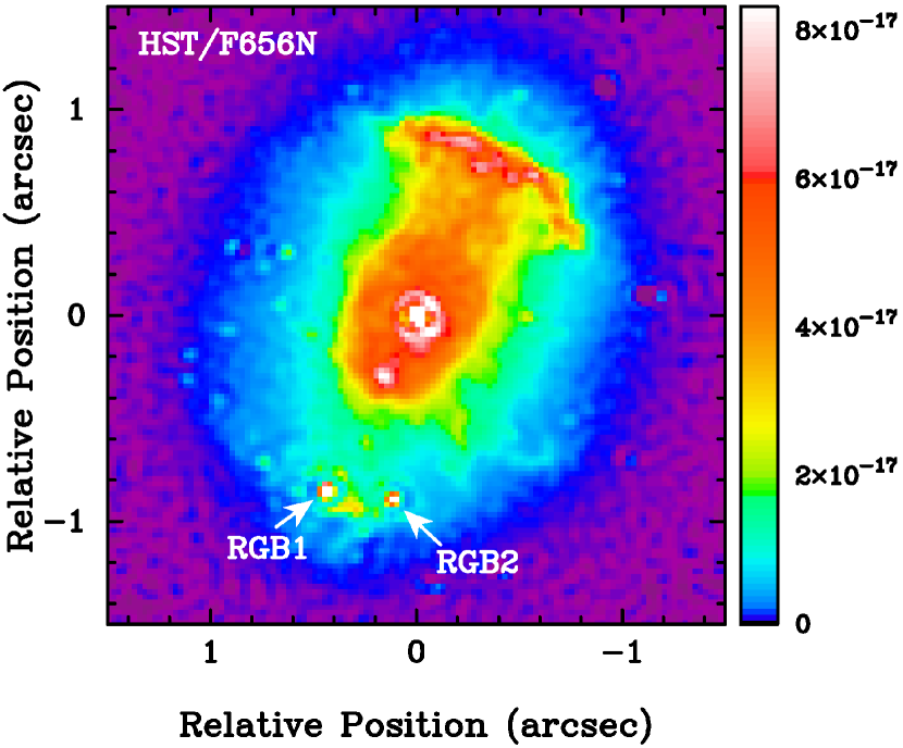
Figure 1.— The H$\alpha$ image of K648 taken by the HST/WFPC2 with the F656N filter. North is up and east is to the left. The intensity is in erg s^-1 cm^-2 Å^-1. Bright stars close to K648 are subtracted out. See Section 2.4 for details of the methods employed. The locations of two RGB stars are indicated by the arrows. The reddening corrected magnitudes are 17.35 ($B$) and 16.78 ($V$) in RGB1 and 17.54 ($B$) and 17.11 ($V$) in RGB2, respectively.

It would be interesting to study whether an increased mass star would evolve into a C-rich PN through such an evolutionary route. In AGB nucleosynthesis models, the predicted abundances, in particular $n$-capture elements, depend on the TDU efficiency, the number of thermal pulses, and the ¹³C pocket mass. Any $n$-capture elements have not yet been detected in K648. The Ne abundance is also sensitive to the amount of ¹³C pocket mass (Shingles & Karakas, 2013). The Ne abundances can be easily determined using atomic gas phase emissions from the PNe rather than stellar absorption. To obtain a detailed view of the origin and evolution of K648 through comparison with AGB nucleosynthesis models, we must accurately determine the abundances of C, O, Ne, and $n$-capture elements, and estimate the ejected mass. K648 is an ideal laboratory in which to investigate the evolution of low-mass metal-poor stars, as well as their nucleosynthesis. The reasons for this are first that the upper mass limit of stars in M15 is known ($\lesssim$1.6 $M_{\odot}$), and second that, because the distances are known with relatively little uncertainty, it is possible to determine the core-mass of the PN as well as of the ejected mass. Study of K648 benefits not only understanding of the evolution of low-mass metal-poor stars, but also dust production in these stars.

In this paper, we describe detailed spectroscopic analyses of K648 to investigate the origin and evolution of this PN based on an extensive set of spectroscopic/photometric data from the far-UV to far-infrared (FIR) regions of the electromagnetic spectrum. The remainder of the paper is organised as follows. In Section 2, we describe these observations using the Subaru/HDS, HST/WFPC2/FOS/COS, Spitzer/IRS/IRAC/MIPS, and Herschel/PACS. In Section 3, we provide the elemental abundances of the nebula and the CSPN, as well as the physical properties of the CSPN. We determined the abundances of the 10 elements of the nebula of K648, including the first measurements of the $n$-capture element fluorine (F) in this PN. Using the spectrum synthesis code TLUSTY (Lanz & Hubeny, 2003), we determined the abundances of 7 elements of the CSPN and the core-mass of the CSPN. We also report the C-rich dust features found in the Spitzer/IRS spectrum. We constructed a self-consistent model, whereby the predicted spectral energy distribution (SED) fits the observations and accordingly estimated the mass of ejected gas and dust using the radiative transfer code CLOUDY (Ferland et al., 1998). In Section 4, we compare the elemental abundances of K648 with those of H4-1 and BoBn1. We discuss the origin and evolution of K648 by comparing the predicted elemental abundances, the final core-mass, and the ejected mass reported by Lugaro et al. (2012) with our determined values. A summary is presented in Section 5.

2. Observations & data reduction

2.1. HDS observations

Figure 2.— The de-reddened HDS spectrum of K648. The wavelength is corrected to the rest wavelength in air.

Optical high-dispersion spectra were obtained using a High-Dispersion Spectrograph (HDS; Noguchi et al., 2002) attached to the Nasmyth focus of the 8.2-m Subaru telescope on 2012 June 28 (Program ID: S12A-078, PI: M. Otsuka).

The weather conditions were stable and clear throughout the night, and the seeing was $\sim$0.5″ measured using the guider CCD. An atmospheric dispersion corrector (ADC) was used to minimize the differential atmospheric dispersion throughout the broad wavelength region. The slit width was set to 1.2″ and the slit length was set to 6″; these settings allowed us to reduce contamination from nearby stars. We selected 2$\times$2 on-chip binning. The resolving power ($R$) was 33 500, determined from the average full-width at half-maximum (FWHM) of over 600 Th-Ar comparison lines. Blue-cross and the red-cross dispersers were employed to obtain the 3620-5400 Å spectrum (blue spectrum) and the 4320-7140 Å spectrum (red spectrum), respectively. We set the position angle to –27^∘ using an image de-rotator. The total exposure times were 7200 s for the blue spectrum and 9000 s for the red spectrum, respectively. Flux calibration, blaze function correction and airmass correction were carried out by observing the standard star BD+28^∘ 4211 twice at different airmasses for each blue and red spectrum.

Data reduction was carried out using the Echelle Spectra Reduction Package ECHELLE in IRAF. We generated a single 3620-7140 Å spectrum by combining the blue and the red spectra after scaling the flux density of the blue spectrum by a factor of 1.06 to match that of the red spectrum. The resulting signal-to-noise (S/N) ratio was $>$50-130 for the continuum of this single 3620-7140 Å spectrum.

Figure 2 shows the resulting spectrum, which is corrected for interstellar extinction (see the following section). The observed wavelength was corrected to the averaged line-of-sight heliocentric radial velocity of –116.89$\pm$0.41 km s^-1 (the root mean square (RMS) of the residuals was 4.15 km s^-1) among all lines detected in the HDS spectrum (122 lines).

2.2. Interstellar reddening correction of the HDS spectrum

The line-fluxes were de-reddened using the follow expression:

$$I(\lambda)=F(\lambda)\times 10^{c({\rm H}\beta)(1+f(\lambda))},$$ (1)

where $I$($\lambda$) is the de-reddened line flux, $F$($\lambda$) is the observed line flux, $f$($\lambda$) is the interstellar extinction function at $\lambda$ computed by the reddening law reported by Cardelli et al. (1989) with $R_{V}$ = 3.1, and $c$(H$\beta$) is the reddening coefficient at H$\beta$. Our measured $F$(H$\beta$) was 1.70$\times$10^-12$\pm$3.14$\times$10^-14 erg s^-1 cm^-2 in the HDS spectrum. Hereafter, X(–Y) corresponds to X$\times$10^-Y. We computed $c$(H$\beta$) by comparing the observed Balmer line ratios of H$\gamma$ and H$\alpha$ to H$\beta$ with the theoretical ratios reported by Storey & Hummer (1995) with an electron temperature of $T_{\epsilon}$ = 10⁴ K and an electron density of $n_{\epsilon}$ = 10⁴ cm^-3 with the assumptions of Case B. The values of $c$(H$\beta$) were 0.121$\pm$0.027 from the $F$(H$\gamma$)/$F$(H$\beta$) and 0.148$\pm$0.008 from the $F$(H$\alpha$)/$F$(H$\beta$) ratios. We used an average value of $c$(H$\beta$) = 0.135$\pm$0.017 for the interstellar reddening correction.

2.3. Emission-line flux measurements with the HDS spectrum

The detected emission-lines are given in the Appendix (see Table A). For the flux measurements, we applied multiple Gaussian component fitting. We list the observed wavelength and de-reddened relative fluxes for each Gaussian component (indicated by Comp.ID number in the fourth and the eleventh columns of Table A in the Appendix), with respect to the de-reddened H$\beta$ flux of 100. $f$($\lambda$) for each wavelength is also listed. Most of the line-profiles of the detected lines can be fitted using a single Gaussian component. For the lines composed of multiple components, e.g., [O ii] $\lambda$ 3726.03 Å, we list the de-reddened relative fluxes of each component, as well as the sum of these components (indicated by Tot.).

We supplemented our HDS data with the data given by Tajitsu & Otsuka (2006) to calculate the Ar²⁺ abundance using [Ar iii] $\lambda$ 7135 Å, $T_{\epsilon}$([O ii]) and $n_{\epsilon}$([O ii]) by combining [O ii] $\lambda\lambda$ 7320/30 Å with [O ii] $\lambda\lambda$ 3726/29 Å, and $T_{\epsilon}$(He i) using He i $\lambda$ 7281 Å.

2.4. HST/WFPC2 photometry and the H$\alpha$/H$\beta$ fluxes

Table 1HST/WFPC2 photometry data for K648.

			CSPN+Nebula		CSPN
Filter	$\lambda_{\rm cen.}$	$\Delta$$\lambda$	$F_{\lambda}$	$I_{\lambda}$	$F_{\lambda}$	$I_{\lambda}$	Prop.ID
	(Å)	(Å)	(erg s-1 cm-1 Å-1)	(erg s-1 cm-1 Å-1)	(erg s-1 cm-1 Å-1)	(erg s-1 cm-1 Å-1)
F160BW	1515.16	188.43	1.05(–13)$\pm$2.54(–15)	2.09(–13)$\pm$5.09(–15)	$\cdots$	$\cdots$	11975
F170W	1820.78	285.52	9.72(–14)$\pm$9.01(–16)	1.89(–13)$\pm$1.75(–15)	9.54(–14)$\pm$7.67(–15)	1.85(–13)$\pm$1.49(–14)	11975
F255W	2598.57	171.21	3.01(–14)$\pm$3.95(–16)	5.29(–14)$\pm$6.95(–16)	$\cdots$	$\cdots$	10524
F300W	2989.04	324.60	2.19(–14)$\pm$2.16(–15)	3.54(–14)$\pm$3.48(–15)	1.43(–14)$\pm$1.28(–15)	2.30(–14)$\pm$2.06(–15)	11975
F336W	3359.48	204.49	2.32(–14)$\pm$3.30(–15)	3.56(–14)$\pm$5.06(–15)	1.76(–14)$\pm$4.94(–16)	2.71(–14)$\pm$7.58(–16)	6751
F439W	4312.09	202.32	1.11(–14)$\pm$4.19(–15)	1.58(–14)$\pm$5.98(–15)	9.97(–15)$\pm$3.46(–16)	1.42(–14)$\pm$4.93(–16)	6751
F547M	5483.88	205.52	4.62(–15)$\pm$9.57(–16)	6.01(–15)$\pm$1.24(–15)	3.84(–15)$\pm$1.04(–16)	4.99(–15)$\pm$1.35(–16)	6751
F814W	7995.94	646.13	1.57(–15)$\pm$2.97(–16)	1.84(–15)$\pm$3.47(–16)	1.24(–15)$\pm$5.01(–17)	1.45(–15)$\pm$5.86(–17)	6751
F656N	6563.76	53.78	1.04(–13)$\pm$4.33(–16)	1.28(–13)$\pm$5.37(–16)	$\cdots$	$\cdots$	6751

Note. — $F_{\lambda}$ and $I_{\lambda}$ are the reddened and de-reddened flux densities, respectively. We used the reddening law reported by Cardelli et al. (1989) for interstellar reddening correction with $R_{\rm V}$ = 3.1 and $E(B-V)$ = 0.092.

In the FOS UV-spectrum (see the following section), no H i or He ii nebular lines are required to normalize the C iii] and [C ii] fluxes to the H$\beta$ flux. Therefore, we measured the H$\beta$ flux of the entire nebula and scaled the FOS flux density to tune the UV flux densities at bands including the C iii] $\lambda\lambda$ 1906/09 Å and the [C ii] $\lambda$ 2323 Å lines. The H$\beta$ flux of the entire nebula is also necessary to normalize the fluxes of the lines detected in the Spitzer/IRS spectrum (see the following section). Broadband fluxes are required to estimate the core-mass of the CSPN and to constrain the incident SED of the CSPN and the emergent spectra predicted by the nebular model. For this purpose, we used HST/Wide Field and Planetary Camera 2 (WFPC2) photometry using eight broadband and F656N filters, which are available in the Mikulski Archive for Space Telescopes (MAST).

We reduced the WFPC2 data (IDs:10524 and 11975, PI:F. R. Francesco; ID:6751, PI: H. E. Bond) using the standard HST pipeline and MultiDrizzle on PYRAF to remove cosmic-rays and improve the angular resolution. First, we removed nearby stars using empirical point-spread functions (PSFs) generated from IRAF/DAOPHOT. We then measured the count rates (cts) within an aperture radius of 2.1″. We defined the background sky as being represented by an annulus centered on the CSPN with inner radius of 3.2″ and outer radius of 4.2″. Finally, we converted the cts into the flux densities using the PHOTFLAM values in erg s^-1 cm^-2 Å^-1 cts^-1. The resulting flux densities $F_{\lambda}$ and the corresponding de-reddened data $I_{\lambda}$ are listed in the fourth and fifth columns of Table 1.

To measure the H$\alpha$ flux of the entire nebula using the F656N flux density, it is necessary to remove the contributions of both the local continuum and the [N ii] $\lambda$ 6548 Å line. However, this procedure entails a number of problems (see e.g., Luridiana et al. (2003) for a thorough discussion of the pitfalls and uncertainties in determining line-fluxes from HST/WFPC2 images for the PN NGC6543). An alternative is to use an intermediate step of computing an equivalent H$\alpha$ flux, that is, using the Spitzer H i Pf$\alpha$ and Hu$\alpha$ recombination lines. This method also has problems of contamination due to the 7.7 $\mu$m PAH feature, as well as the broad 11 $\mu$m feature, and the [Ne ii] $\lambda$ 12.80 $\mu$m line in the Spitzer spectra. Rather than employing the above HST H$\alpha$ flux extraction method, or the intermediate step of using Spitzer H i lines, we used the HST/WFPC2 F656N band flux density itself, i.e., $F_{\lambda}$(HST,F656N), which includes the H$\alpha$ flux, the local continuum, and the [N ii] $\lambda$6548 Å line within the F656N filter band, together with our Subaru/HDS spectrum. The advantage of this approach is that it is possible to extract the H$\alpha$ flux without contamination from nebular and stellar continuum and [N ii] $\lambda$6548 Å. This method was applied in our previous work on the PN M1-11 (Otsuka et al., 2013). Taking into account the F656N filter transmission characteristics, we compared the $F_{\lambda}$(HST,F656N) with the counterpart Subaru/HDS scan spectrum, i.e., $F_{\lambda}$(HDS,F656N). The scaling factor $F_{\lambda}$(HST,F656N)/$F_{\lambda}$(HDS,F656N) = 1.428 was determined, and was applied to the Subaru/HDS spectral line fluxes to analyze both the spectra on an equal footing. After applying the scaling factor, the HDS fluxes should be $F$(H$\alpha$) = 2.42(–12)$\pm$4.44(–14) erg s^-1 cm^-2 and $F$(H$\beta$) = 7.83(–13)$\pm$1.05(–15) erg s^-1 cm^-2. A simple comparison of these scaled HDS data with the measured HST data shows very small deviations, i.e., 0.18%, & 0.13%, corresponding to the H$\alpha$ and H$\beta$ fluxes measured from non-scaled HDS spectrum. The uncertainties of our measurements are much smaller than the estimated uncertainty of $\sim$10% reported by Luridiana et al. (2003). These reduced errors may be coincidental and the actual errors could be larger than our estimation; however, the errors in our analysis appear to be smaller than the estimates reported by Luridiana et al. (2003). The scaling factors also give ratios of Pf$\alpha$ and Hu$\alpha$ with the above H$\beta$ fluxes that are consistent with the theoretical values (see Section 2.7). Note that the Spitzer/IRS spectra were obtained using a wider slit width, which was sufficient to cover the entire K648 nebula.

2.5. HST/FOS UV-spectrum

Table 2The detected lines in the HST/FOS spectra.

$\lambda_{\rm obs}$	Ion	$\lambda_{\rm lab}$	Comp.	$f$($\lambda$)	$I$($\lambda$)a
(Å)		(Å)			[$I$(H$\beta$) = 100]
1906.83	C iii]	1906/09	1	1.256	334.984$\pm$17.038
2326.45	[C ii]	2323	1	1.392	17.091$\pm$1.634

To calculate the C²⁺ and C⁺ abundances using the C iii] $\lambda\lambda$ 1906/09 Å and the [C ii] $\lambda$ 2323 Å lines, we analyzed the archival HST/FOS spectrum (The Faint Object Spectrograph), which was obtained on 1993 Nov 18 (Prop.ID: 3196, PI: H. Ford), and was downloaded from MAST. We used the data sets Y1C40103P, Y1C40104T, Y1C40105T, and Y1C40106T.

We scaled the flux density to fit the F160BW, F170W, and F255W bands listed in the fourth column of Table 1 using the relevant transmission curves (scaling factor = 0.837). Using the $F$(H$\beta$) = 7.83(–13)$\pm$1.05(–15) erg s^-1 cm^-2, we normalized the C iii] $\lambda\lambda$ 1906/09 Å and the [C ii] $\lambda$ 2323 Å fluxes.

2.6. FUSE and HST/COS UV-spectra

We analyzed archival UV spectra of K648 from MAST to calculate the elemental abundances in the photosphere of the CSPN and determine the parameters required to calculate the stellar radius, surface gravity $\log$ $g$, effective temperature $T_{\rm eff}$, and the current core-mass of the CSPN. The 920-1180 Å and the 1170-1780 Å spectra were obtained using the Far Ultraviolet Spectroscopic Explorer (FUSE) on 2004 Nov 1 (data set: D1570101000, PI: Dixon) for and the HST/Cosmic Origins Spectrograph (COS) on 2013 Nov 13 (data set: LB2402010/20; Prop-ID:11527, PI: J. Green). We generated the FUSE, HST/COS, and HDS spectra normalized to the flux density at a continuum of 1.0 using IRAF/SPLOT.

2.7. Spitzer/IRS mid-infrared spectra

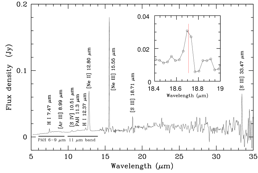
Figure 3.— The Spitzer/IRS spectrum of K648. The detected gas emission lines listed in Table 3 are also indicated here. The 6-9 ${\mu}$m PAH band, the 11.3 ${\mu}$m PAH emission, and the broad 11 ${\mu}$m band are also indicated. The line-profile of the [S iii] $\lambda$ 18.71 $\mu$m is zoomed in the inner box. The position of this line in the laboratory is indicated by the vertical red line.

Table 3The detected atomic lines in the Spitzer spectra.

$\lambda_{\rm lab}$	Ion	$f$($\lambda$)	$F$($\lambda$)	$I$($\lambda$)
($\mu$m)			(erg s-1 cm-2)	[$I$(H$\beta$) = 100]
7.47	H i	–0.990	3.23(–14)$\pm$1.56(–16)	3.15$\pm$0.15
8.99	[Ar iii]	–0.959	3.29(–15)$\pm$4.84(–16)	0.32$\pm$0.05
10.51	[S iv]	–0.959	1.08(–14)$\pm$4.46(–16)	1.06$\pm$0.07
12.37	H i	–0.980	1.04(–14)$\pm$5.17(–16)	1.02$\pm$0.07
12.80	[Ne ii]	–0.983	1.53(–13)$\pm$1.08(–14)	14.98$\pm$1.28
15.55	[Ne iii]	–0.985	1.18(–13)$\pm$1.42(–14)	11.54$\pm$1.49
18.71	[S iii]	–0.981	1.36(–14)$\pm$1.98(–15)	1.33$\pm$0.20
33.47	[S iii]	–0.993	6.27(–15)$\pm$1.12(–15)	0.61$\pm$0.11

We reduced the archive data obtained using the Infrared Spectrograph (IRS; Houck et al., 2004) with the SL (5.2-14.5 $\mu$m and a slit dimension of 3.6″$\times$57″), SH (9.9-19.6 $\mu$m, 4.7″$\times$11.3″), and LH (18.7-37.2 $\mu$m, 11.1″$\times$22.3″) modules (AOR Keys: 15733760 for the SL and 18627840 for the SH and LH spectra; PIs: R. Gehrz and J. Bernard-Salas, respectively). We used the data reduction packages SMART v.8.2.5 (Higdon et al., 2004) and IRSCLEAN provided by the Spitzer Science Center. For the SH and the LH spectra, we subtracted the background sky using the offset spectra. We scaled the flux density of the SL data to that of the SH & LH data in the overlapping wavelength region. The remaining spikes in the spectra were removed manually.

The resulting spectrum is shown in Fig. 3. Boyer et al. (2006) reported the SL spectrum for K648 only. Therefore, the spectrum at longer wavelengths (i.e., beyond $\sim$14.5 $\mu$m) is shown here for the first time. The line-profile of the [S iii] $\lambda$ 18.71 ${\mu}$m, which is faint in K648 and also a important diagnostic line, is also shown in the inner box.

The line fluxes of the detected atomic lines are listed in Table 3. We corrected for the interstellar reddening using Equation (1) and the interstellar extinction function given by Fluks et al. (1994). We computed $c$(H$\beta$) = 0.12$\pm$0.02 by comparing the theoretical $I$(H i 7.47 $\mu$m)/$I$(H$\beta$) ratio of 3.15(–2) given by Storey & Hummer (1995) for $T_{\epsilon}$ = 10⁴ K and $n_{\epsilon}$ = 10⁴ cm^-3 under the assumptions of Case B. Here, we used $F$(H$\beta$) = 7.83(–13) erg s^-1 cm^-2 (see Section 2.4). This result appears appropriate as the measured $I$(H i 12.37 $\mu$m)/$I$(H$\beta$) = 1.02(–2) is in good agreement with the theoretical data (1.05(–2), Storey & Hummer, 1995).

K648 exhibits the 6-9 $\mu$m polycyclic amorphous carbon (PAH) band and the broad 11 $\mu$m feature. These two features are frequently seen in C-rich PNe. We will discuss the details on these features in Section 3.3.

2.8. Spitzer/IRAC/MIPS photometry

Table 4Spitzer/IRAC/MIPS and Herschel/PACS photometry of K648.

Band	$\lambda_{\rm cen.}$	$\Delta$$\lambda$	$F_{\lambda}$	AORKEY(Spitzer)/
	($\mu$m)	($\mu$m)	(erg s-1 cm-1 $\mu$m-1)	OBSID(Herschel)
IRAC-ch1	3.51	0.68	1.24(–12)$\pm$1.53(–13)	12030208
IRAC-ch2	4.50	0.86	6.16(–13)$\pm$4.80(–14)	12030208
IRAC-ch3	5.63	1.26	4.78(–13)$\pm$4.51(–14)	12030208
IRAC-ch4	7.59	2.53	4.43(–13)$\pm$2.82(–14)	12030208
MIPS-ch1	23.21	5.30	5.95(–14)$\pm$1.44(–15)	12030464
PACS-B	68.92	21.41	1.86(–15)$\pm$3.82(–17)	1342246710/11/12
PACS-R	153.94	69.76	3.40(–16)$\pm$4.00(–17)	1342246710/11/12

To provide a constraint in the SED fitting at mid-infrared (MIR) wavelengths, we reduced archival Spitzer MIR images obtained using the Infrared Array Camera (IRAC; Fazio et al., 2004) and the Multiband Imaging Spectrometer (MIPS; Rieke et al., 2004). We downloaded the basic calibrated data and reduced it using MOPEX, which is provided by the Spitzer Science Center, to obtain single mosaic images for each band.

We carried out PSF fitting photometry of the IRAC images using IRAF/DAOPHOT. We adopted the position of K648 measured in the HST/F656N image and corrected the flux densities measured using PSF photometry by aperture photometry of the PSF stars. For the MIPS 24 $\mu$m image, we measured the total count within a 7″ radius region, and subtracted the background represented by the annulus centered on the PN with 20″ inner and 38″ outer radii, respectively. We used an aperture correction factor of 1.61, as listed in the MIPS instrument hand book. The measured fluxes are listed in Table 4.

2.9. Herschel/PACS photometry

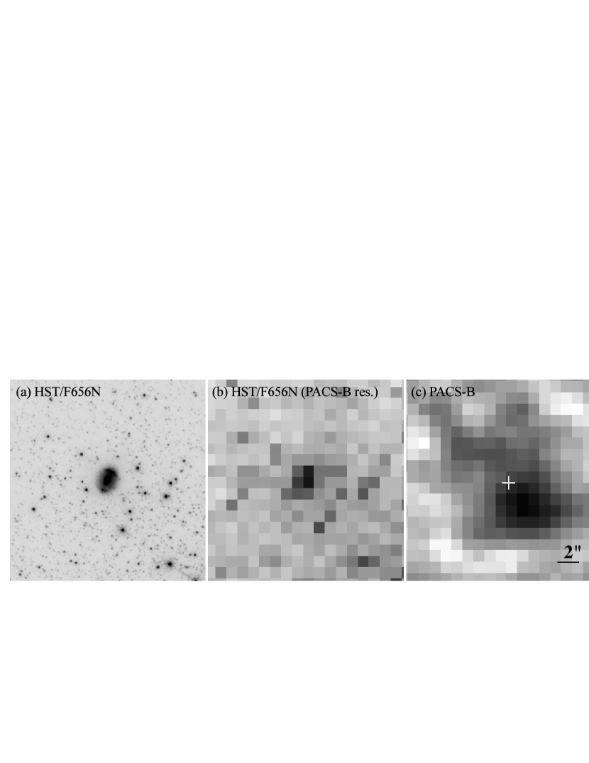
Figure 4.— The HST/F656 and the Herschel/PACS images. The size of each panel is 17${\arcsec}$$\times$17${\arcsec}$. North is up and east is to the left. The plate scale of the image in (a) is 0.025${\arcsec}$ pixel^-1. The plate scale of the HST/F656N image in (b) corresponds to that of PACS-B (1${\arcsec}$ pixel^-1). K648 is located in the center of each image. In the PACS-B and PACS-R images, the location of K648 is indicated by the crosses.

By combining the MIR data from the Spitzer and the FIR data from the Herschel, we attempted to trace the ejected mass of K648 during the last TP as accurately as possible. For this purpose, we analyzed archived 70 $\mu$m (PACS-B) and 160 $\mu$m images (PACS-R) obtained using the Herschel/Photodetecting Array Camera and Spectrometer (PACS; Poglitsch et al., 2010).

We downloaded the reduced PACS data of K648 (OBSID: 1342246710/11/12, PI: M. Boyer) from the Herschel Science Archive (HSA). The PACS images are shown in Fig. 4. For comparison, we also show the HST/F656N images. The plate scale of the image shown in Fig. 4(a) is 0.025${\arcsec}$ pixel^-1 and that of the HST/F656N image shown in Fig. 4(b) corresponds to that of PACS-B. Fig. 4(c) shows PACS-B data at 1${\arcsec}$ pixel^-1, and Fig. 4(d) shows the plate scale of PACS-R at 2${\arcsec}$ pixel^-1. The most likely position of K648 was determined using the HST/F656N image, and is indicated by the white crosses. The light from K648 is partially contaminated by nearby stars.

We used IRAF/DAOPHOT to measure the flux densities within a radius of 2 pixels in both the PACS-B and PACS-R bands. We regarded the median count within the annulus centered on the PN with an inner radius of four pixels and an outer radius of five pixels as the background. We corrected the measured flux densities of K648 using aperture photometry with correction factors of 4.29 for PACS-B and 3.83 for PACS-R. The measured flux densities are summarized in Table 4.

3. Results

3.1. Emission-line analysis

3.1.1 CEL diagnostics

Figure 5.— An $n_{\epsilon}$-$T_{\epsilon}$ diagram. Each curve is labeled with an ID number given in Table 5. The solid lines indicate diagnostic lines of $T_{\epsilon}$, whereas the broken lines indicate diagnostic lines of $n_{\epsilon}$.

Table 5Plasma diagnostics.

ID	Diagnostic	Value	$n_{\epsilon}$ (cm-3)
(1)	$[$S ii$]$($\lambda$6716)/($\lambda$6731)	0.658$\pm$0.023	2530$\pm$330
(2)	$[$O ii$]$($\lambda$3726)/($\lambda$3729)	1.852$\pm$0.076	3430$\pm$470
(3)	$[$S iii$]$($\lambda$18.7 $\mu$m)/($\lambda$33.5 $\mu$m)	2.178$\pm$0.523	5110$\pm$2100
(4)	$[$O ii$]$($\lambda$3726/29)/($\lambda$7320/30)	8.576$\pm$0.108a	7890$\pm$130
(5)	$[$Cl iii$]$($\lambda$5517)/($\lambda$5537)	0.749$\pm$0.120	7130$\pm$3170
	Balmer decrement		7500-10 000
ID	Diagnostic	Value	$T_{\epsilon}$ (K)
(6)	$[$O iii$]$($\lambda$4959+$\lambda$5007)/($\lambda$4363)	108.649$\pm$4.425	12 350$\pm$190
(7)	$[$Ne iii$]$($\lambda$15.5 $\mu$m)/($\lambda$3869+$\lambda$3967)	0.882$\pm$0.115	11 090$\pm$450
(8)	$[$N ii$]$($\lambda$6548+$\lambda$6583)/($\lambda$5755)	79.200$\pm$9.333	10 380$\pm$530
(9)	$[$Ar iii$]$($\lambda$8.99 $\mu$m)/($\lambda$7135)	0.844$\pm$0.125	10 270$\pm$900
	He i($\lambda$5876)/($\lambda$4471)	3.019$\pm$0.033	4270$\pm$300
	He i($\lambda$6678)/($\lambda$4471)	0.837$\pm$0.012	7100$\pm$760
	He i($\lambda$7281)/($\lambda$5876)	0.040$\pm$0.001	6360$\pm$150
	He i($\lambda$7281)/($\lambda$6678)	0.145$\pm$0.003	6680$\pm$130
	(Balmer Jump)/(H11)	0.102$\pm$0.006	11 650$\pm$950

In the following analysis using CELs and RLs, we used the transition probabilities, collisional impacts, and recombination coefficients listed in Tables 7 and 11 of Otsuka et al. (2010).

The electron temperatures and densities were determined using a variety of line diagnostic ratios by calculating the state populations using a multilevel atomic model. The observed diagnostic line ratios are listed in Table 5, where the numbers in the first column indicate the ID of each curve in the $n_{\epsilon}$-$T_{\epsilon}$ diagram shown in Fig. 5. The second, third, and final columns in Table 5 show the diagnostic lines, line ratios, and the resulting $n_{\epsilon}$ and $T_{\epsilon}$, respectively. We obtained nine diagnostic line ratios with different ionization potentials (IPs) in the range 10.4 eV ([S ii]) to 41 eV ([Ne iii]), and determined a suitable $T_{\epsilon}$ and $n_{\epsilon}$ combination for each ion.

For the [O ii] $\lambda\lambda$ 7320/30 Å lines, we eliminated the recombination contamination due to O²⁺ using the following expression, which is given by Liu et al. (2000):

$$\frac{I_{R}(\rm[O\,{\sc II}]\lambda\lambda 7320/30)}{I(\rm H\beta)}=9.36\left(\frac{T_{\epsilon}}{10^{4}}\right)^{0.44}\times\frac{\rm O^{2+}}{\rm H^{+}}.$$ (2)

Using the O²⁺ ionic abundances derived from the recombination O ii $\lambda$ 4641.8 Å line and with $T_{\epsilon}$ = 11 650 K, based on the Balmer jump discontinuity (see the following section), we found that $I_{R}$([O ii] $\lambda\lambda$ 7320/30) = 0.12$\pm$0.02. As we could not detect the N ii and the pure O iii recombination lines, we were unable to estimate the contribution of N²⁺ to the [N ii] $\lambda$ 5755 Å line nor that of O³⁺ to the [O iii] $\lambda$ 4363 Å line.

First, we computed $n_{\epsilon}$ with $T_{\epsilon}$ = 10 000 K for all density diagnostic lines. $T_{\epsilon}$([Ne iii]), $T_{\epsilon}$([O iii]), and $T_{\epsilon}$([Ar iii]) were calculated using $n_{\epsilon}$ = 6100 cm^-3, which is the averaged $n_{\epsilon}$ between $n_{\epsilon}$([Cl iii]) and $n_{\epsilon}$([S iii]). We calculated $T_{\epsilon}$([N ii]) using the $n_{\epsilon}$([O ii]) determined from the [O ii] $I$($\lambda$3726)/$I$($\lambda$3729) ratio. We used [O ii] $I$($\lambda\lambda$3726/29)/$I$($\lambda\lambda$7320/30) as a density indicator for the $\sim$4500 cm^-3 region, which is larger than the critical density of [O ii] $\lambda$ 3726 Å.

Our values of $T_{\epsilon}$ and $n_{\epsilon}$ are comparable to those reported by Kwitter et al. (2003), i.e., $T_{\epsilon}$([O iii]) = 11 800 K, $T_{\epsilon}$([N ii]) = 9200 K, and $n_{\epsilon}$([S ii]) = 1000 cm^-3.

3.1.2 RL diagnostics

Figure 6.— The intensity ratio of the higher-order Balmer lines to H$\beta$ (Case B assumption). The theoretical intensity ratios (dotted curve and triangles) are given for $T_{\epsilon}$ = 11 650 K (determined from the Balmer Jump) and $n_{\epsilon}$ = 10⁴ cm^-3.

We calculated $T_{\epsilon}$ using the ratio of the Balmer discontinuity to $I$(H11). We employed the method reported by Liu et al. (2001) to calculate the electron temperature $T_{\epsilon}$(BJ).

We calculated the He i electron temperatures using the four different $T_{\epsilon}$(He i) line ratios and the emissivities of these He i lines from Benjamin et al. (1999), in the case of $n_{\epsilon}$ = 10⁴ cm^-3.

The intensity ratio of a high-order Balmer line H$n$ (where $n$ is the principal quantum number of the upper level) to a lower-order Balmer line is also sensitive to the electron density. The ratios of higher-order Balmer lines to H$\beta$ are plotted in Fig. 6 along with theoretical values from Storey & Hummer (1995) for $T_{\epsilon}$(BJ) and $n_{\epsilon}$ = 10 000 cm^-3. We ran small-grid calculations to determine $n_{\epsilon}$ in the range 5000-12 500 cm^-3, and found that the models in the range of $n_{\epsilon}$ = 7500-10 000 cm^-3 provided the best fit to the observed data. $T_{\epsilon}$ and $n_{\epsilon}$ determined using the RL diagnostics are summarized in Table 5.

3.1.3 CEL ionic abundances

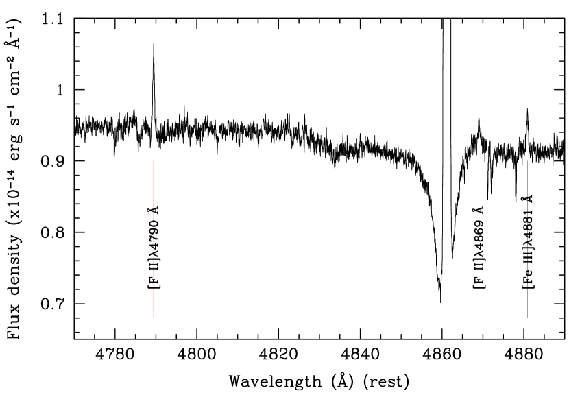
Figure 7.— The 4770-4890 Å Subaru/HDS spectrum of K648. The wavelength is corrected to the rest wavelength in air. The locations of the [F ii] $\lambda\lambda$ 4790/4869 Å lines in are indicated by the vertical red lines. The position of the [Fe iii] $\lambda$4881 Å is indicated by the vertical black line. The narrow absorptions are from cool stars, possibly two nearby RGB stars (see Fig. 1).

Table 6The adopted electron temperatures and densities.

$T_{\epsilon}$ (K)	$n_{\epsilon}$ (cm-3)	Ions
10 380	2530	S+
10 380	3430	C+,N+,O+(3726,29 Å),F+,Fe2+
10 380	7840	O+(7320,30 Å)
10 270	6100	C2+,Ne+,S2+,Cl2+,Ar2+
11 090	6100	Ne2+
12 350	6100	O2+,S3+

Table 7Ionic Abundances from CELs.

Xm+	$\lambda_{\rm lab}$	$I$($\lambda_{\rm lab}$)	Xm+/H+
C+	2323 Å	1.64(+1)$\pm$1.63(0)	2.55(–5)$\pm$7.28(–6)
C2+	1906/09 Å	3.35(+2)$\pm$1.70(+1)	6.91(–4)$\pm$3.23(–4)
N+	5754.64 Å	4.31(–2)$\pm$2.44(–3)	4.67(–7)$\pm$1.02(–7)
	6548.04 Å	9.01(–1)$\pm$1.23(–2)	4.93(–7)$\pm$5.89(–8)
	6583.46 Å	3.18(0)$\pm$4.10(–2)	5.89(–7)$\pm$7.02(–8)
			5.68(–7)$\pm$6.77(–8)
O+	3726.03 Å	1.74(+1)$\pm$2.99(–1)	1.34(–5)$\pm$2.50(–6)
	3728.81 Å	9.39(0)$\pm$3.50(–1)	1.34(–5)$\pm$2.60(–6)
	7320/30 Å	3.12(0)$\pm$3.91(–2)a	1.79(–5)$\pm$4.40(–6)
			1.34(–5)$\pm$2.54(–6)
O2+	4363.21 Å	2.78(0)$\pm$2.56(–2)	4.03(–5)$\pm$3.29(–6)
	4931.23 Å	3.84(–2)$\pm$4.83(–3)	5.12(–5)$\pm$6.80(–6)
	4958.91 Å	7.50(+1)$\pm$7.37(0)	3.90(–5)$\pm$4.18(–6)
	5006.84 Å	2.27(+2)$\pm$9.46(0)	4.09(–5)$\pm$2.45(–6)
			4.05(–5)$\pm$2.89(–6)
F+	4789.45 Å	1.10(–1)$\pm$3.67(–3)	6.67(–8)$\pm$1.02(–8)
	4868.99 Å	2.96(–2)$\pm$3.36(–3)	5.75(–8)$\pm$1.08(–8)
			6.47(–8)$\pm$1.03(–8)
Ne+	12.80 $\mu$m	1.50(+1)$\pm$1.28(0)	2.01(–5)$\pm$1.95(–6)
Ne2+	3869.06 Å	9.94(0)$\pm$1.24(–1)	7.28(–6)$\pm$1.00(–6)
	3967.79 Å	3.15(0)$\pm$4.35(–2)	7.65(–6)$\pm$1.06(–6)
	15.55 $\mu$m	1.13(+1)$\pm$1.36(0)	7.48(–6)$\pm$9.79(–7)
			7.42(–6)$\pm$9.98(–7)
S+	6716.44 Å	8.73(–2)$\pm$2.23(–3)	6.72(–9)$\pm$7.79(–10)
	6730.81 Å	1.33(–1)$\pm$3.21(–3)	6.73(–9)$\pm$7.48(–10)
			6.72(–9)$\pm$7.60(–10)
S2+	6313.1 Å	1.19(–1)$\pm$5.12(–3)	2.52(–7)$\pm$7.30(–8)
	18.71 $\mu$m	1.33(0)$\pm$2.04(–1)	2.10(–7)$\pm$3.52(–8)
	33.47 $\mu$m	6.12(–1)$\pm$1.13(–1)	2.10(–7)$\pm$4.16(–8)
			2.12(–7)$\pm$3.93(–8)
S3+	10.51 $\mu$m	1.06(0)$\pm$6.66(–2)	3.35(–8)$\pm$2.11(–9)
Cl2+	5517.72 Å	2.12(–2)$\pm$2.71(–3)	3.15(–9)$\pm$7.86(–10)
	5537.89 Å	2.83(–2)$\pm$2.73(–3)	3.17(–9)$\pm$7.38(–10)
			3.16(–9)$\pm$7.59(–10)
Ar2+	7135.79 Å	3.84(–1)$\pm$6.20(–3)	3.32(–8)$\pm$5.73(–9)
	8.99 $\mu$m	3.24(–1)$\pm$4.77(–2)	3.41(–8)$\pm$5.32(–9)
			3.36(–8)$\pm$5.54(–9)
Fe2+	4701.53 Å	2.22(–2)$\pm$3.11(–3)	2.37(–8)$\pm$4.80(–9)
	4881.11 Å	5.09(–2)$\pm$3.55(–3)	2.75(–8)$\pm$4.59(–9)
			2.63(–8)$\pm$4.65(–9)

We obtained the following 14 ionic abundances: C^+,2+, N⁺, O^+,2+, F⁺, Ne^+,2+, S^+,2+,3+, Cl²⁺, Ar²⁺ and Fe²⁺. The abundances of F⁺, Cl²⁺, and Fe²⁺ abundances for K648 are reported here for the first time. The ionic abundances were calculated by solving the statistical equilibrium equations for more than five levels with the relevant $T_{\epsilon}$ and $n_{\epsilon}$, except for Ne⁺, where we calculated the abundance using a two-energy level model. The Fe²⁺ abundances were solved using a 33-level model (from ${}^{5}D_{3}$ to ${}^{3}P_{2}$). For each ion, we used the electron temperatures and densities determined using CEL plasma diagnostics. The adopted $T_{\epsilon}$ and $n_{\epsilon}$ for each ion are listed in Table 6.

The ionic abundances are listed in Table 7. The final column shows the resulting ionic abundances, X^m+/H⁺, together with the relevant errors, including errors from line-intensities, electron temperature, and electron density. The ionic abundance and the error are listed in the final row for each ion. These data were calculated based on the weighted mean of the relevant line-intensity.

In calculation of the C⁺ abundance, we subtracted contamination from [O iii] $\lambda$ 2321 Å to [C ii] $\lambda$ 2323 Å based on the theoretical intensity ratio [O iii] $I$($\lambda$ 2326)/$I$($\lambda$ 4363) = 0.236. As described above, we did not remove the respective contributions from N²⁺ and O³⁺ to the [N ii] $\lambda$ 5755 Å and the [O iii] $\lambda$ 4363 Å line intensities. To determine the final O⁺ abundance, we excluded data determined using the [O ii] $\lambda\lambda$ 7320/30 Å lines.

We determined the Ne⁺ abundance of 2.01(–5) using the [Ne ii] $\lambda$ 12.80 $\mu$m line, which is slightly larger than Boyer et al. (2006, 1.53(–5)). This small disagreement is expected to be mainly due to the adopted H$\beta$ flux. Boyer et al. (2006) calculated the H$\beta$ flux using the measured H i lines at 7.47 $\mu$m and 12.37 $\mu$m, using the theoretical ratios of H i $I$($\lambda$ 7.47 $\mu$m,12.37 $\mu$m)/$I$(H$\beta$) with Case B. Their resulting $I$(H$\beta$) was 1.52$\times$10^-12 erg s^-1 cm^-2. While, we used the HST/F656N band-pass flux intensity and corresponding HDS spectral scan to scale the intensities, and find $I$(H$\beta$) = 1.07$\times$10^-12 erg s^-1 cm^-2. Boyer et al. (2006) used $T_{\epsilon}$ = 10 000 K and $n_{\epsilon}$ = 1700 cm^-3 for the Ne⁺ and S^2+,3+ calculations. Our plasma diagnostics showed that 10 000 K is low for S³⁺, where we used 12 350 K.

The S²⁺ abundance of 2.17(–7) determined using the two MIR [S iii] lines is approximately the same as that calculated from [S iii] $\lambda$ 6312 Å, and is in good agreement with Kwitter et al. (2003), who calculated 1.99(–7) using $I$([S iii] $\lambda$ 9532 Å) = 3.8. However, there was poor agreement in the S²⁺ abundance between the most recent measurements by Boyer et al. (2006, 2.55(–8)) and our data. Boyer et al. (2006) calculated the S²⁺ abundance using $I$([S iii] $\lambda$ 9532 Å) = 0.76 measured by Barker (1983), because they used the Spitzer SL module spectra only, where no MIR [S iii] lines appear. We can exclude the possibility that the discrepancy in the S²⁺ abundance is due to the flux measurements of our MIR [S iii] and the choice of $T_{\epsilon}$. If our flux measurements of the MIR [S iii], [S iii] $\lambda$ 6312 Å and the H$\beta$ lines and the $T_{\epsilon}$ selection were incorrect, the S²⁺ abundances from two MIR [S iii] lines would not match that from [S iii] $\lambda$ 6312 Å. The fine-structure lines are much less sensitive to the electron temperature compared with the other transition lines. The auroral lines, such as [S iii] $\lambda$ 6312 Å, were dependent on the electron temperature (i.e., the S²⁺ abundance determined from [S iii] $\lambda$ 6312 Å is largely dependent on $T_{\epsilon}$). Our calculated S²⁺ abundances from these three were consistent with each other, indicating that our flux measurements of the MIR [S iii] and H$\beta$ lines and the choice of $T_{\epsilon}$ for the S²⁺ (and possibly also Ne⁺ and S³⁺) were appropriate. Therefore, the large discrepancy in S²⁺ between Boyer et al. (2006) and our data may have been due to the [S iii] $\lambda$ 9532 Å flux that was used.

It is interesting to note the detection of single isotope ¹⁹F line candidates [F ii] $\lambda\lambda$ 4789.45/4868.99 Å, as shown in Fig. 7. Together with ¹²C and ²²Ne, ¹⁹F is synthesized in the He-rich intershell during the TP-AGB phase, and is an $n$-capture element. The observed [F ii] $I$($\lambda$ 4789.45)/$I$($\lambda$ 4868.99) of 3.72$\pm$0.44 is in agreement with the theoretical value of 3.20 calculated using $T_{\epsilon}$ = 10 380 K and $n_{\epsilon}$ = 3430 cm^-3. We excluded the other candidate C iv $\lambda$ 4789.65 Å because no C iv lines were detected (e.g., C iv $\lambda$ 5801.35 Å). Therefore, we conclude that the lines at 4790 and 4869 Å are the [F ii] $\lambda\lambda$ 4789.45/4868.99 Å, respectively. The detection of F lines is very rare in Galactic PNe (e.g., Otsuka et al., 2008; Zhang & Liu, 2005; Liu, 1998). Among halo PNe, K648 is the third case of such F line detection reported to date; NGC4361 (Liu, 1998), BoBn1 (Otsuka et al., 2008), and K648 (this work). We discuss whether these lines are $[$F ii$]$ $\lambda\lambda$ 4789.45/4868.99 Å using a theoretical model later in the paper. If the two lines do not originate from the F⁺ ion, the prediction cannot fit the fluxes of the two lines simultaneously.

3.1.4 RL ionic abundances

Table 8Ionic abundances from RLs.

Xm+	$\lambda_{\rm lab}$	Multi.	$I$($\lambda_{\rm lab}$)	Xm+/H+
He+	5875.62 Å	V11	1.48(+1)$\pm$1.38(–1)	1.02(–1)$\pm$6.69(–3)
	4471.47 Å	V14	4.91(0)$\pm$2.78(–2)	9.86(–2)$\pm$6.05(–3)
	6678.15 Å	V46	4.11(0)$\pm$5.48(–2)	9.90(–2)$\pm$6.48(–3)
	4921.93 Å	V48	1.29(0)$\pm$5.28(–3)	9.54(–2)$\pm$5.92(–3)
	4387.93 Å	V51	5.17(–1)$\pm$1.04(–2)	8.34(–2)$\pm$6.66(–3)
				1.00(–1)$\pm$6.49(–3)
C2+	6578.05 Å	V2	6.92(–1)$\pm$1.08(–2)	8.42(–4)$\pm$1.33(–4)
	4267.18 Å	V6	7.26(–1)$\pm$1.33(–2)	7.32(–4)$\pm$9.10(–5)
	6151.27 Å	V16.04	4.50(–2)$\pm$2.89(–3)	1.04(–3)$\pm$1.31(–4)
	6462.04 Å	V17.04	9.81(–2)$\pm$8.62(–3)	9.67(–4)$\pm$1.63(–4)
				8.04(–4)$\pm$1.15(–4)
C3+	6727.48 Å	V3	3.71(–2)$\pm$2.74(–3)	2.05(–4)$\pm$1.48(–5)
	6742.15 Å	V3	4.14(–2)$\pm$3.78(–3)	2.75(–4)$\pm$2.52(–5)
	6744.39 Å	V3	6.05(–2)$\pm$2.80(–3)	2.87(–4)$\pm$1.37(–5)
				2.62(–4)$\pm$1.74(–5)
O2+	4641.81 Å	V1	3.34(–2)$\pm$3.45(–3)	1.21(–4)$\pm$1.64(–5)

The RL ionic abundances are listed in Table 8. As we detected C ii,iii and O ii RLs, we can compare the elemental C and O abundances determined using RLs with those from CELs in K648.

In the abundance calculations, we used the Case B assumption for lines with levels that have the same spin as the ground state, and the Case A assumption for lines of other multiplicities. In the final line of each ion series, we give the ionic abundance and the error estimated using the line intensity weighted mean. As the RL ionic abundances were not sensitive to the electron density with $\lesssim$10⁸ cm^-3, we used the atomic data in the case of $n_{\epsilon}$ = 10⁴ cm^-3 for all lines. To calculate the He⁺ abundances, we used $T_{\epsilon}$(He i) = 6710$\pm$350 K, and the average of all $T_{\epsilon}$(He i) data listed in Table 5, except for $T_{\epsilon}$(He i), where we used the He i $I$($\lambda$ 5876)/$I$($\lambda$ 4471) ratio, which was smaller than the other data. We used the $T_{\epsilon}$(BJ) to calculate the C^2+,3+ and O²⁺ abundances.

We used the multiplet V1 O ii $\lambda$ 4641.81 Å line only, because the observed HDS spectra were partially contaminated by the absorption lines of the CSPN. According to Peimbert et al. (2005), the upper levels of the transitions in the V1 O ii line are not in local thermal equilibrium (LTE) for $n_{\epsilon}$ $<$10 000 cm^-3. As the value of $n_{\epsilon}$ calculated using the Balmer decrement method was 7500-10 000 cm^-3, we applied the non-LTE corrections using Equations (8)-(10) in Peimbert et al. (2005) with $n_{\epsilon}$ = 7500 cm^-3.

3.1.5 Nebular ICF abundances

Table 9The ionization correction factors (ICFs).

X	Line	ICF(X)	X/H
He	RL	$\rm\frac{S^{+}+S^{2+}}{S^{2+}}$	ICF(He)$\rm He^{+}$
C	CEL	$\rm\left(\frac{C}{C^{2+}}\right)_{RL}$	C++ICF(C)C2+
	RL	$\rm\left(\frac{C^{+}+C^{2+}}{C^{2+}}\right)_{CEL}$	ICF(C)C2++C3+
N	CEL	$\rm\left(\frac{O}{O^{+}}\right)_{CEL}$	ICF(N)N+
O	CEL	1	O++O2+
	RL	$\rm\left(\frac{O}{O^{2+}}\right)_{CEL}$	ICF(O)O2+
F	CEL	$\rm\left(\frac{O}{O^{+}}\right)_{CEL}$	ICF(F)F+
Ne	CEL	1	Ne++Ne2+
S	CEL	1	$\rm S^{+}+S^{2+}+S^{3+}$
Cl	CEL	$\rm{\left(\frac{Ar}{Ar^{2+}}\right)}$	ICF(Cl)Cl2+
Ar	CEL	$\rm\frac{S}{S^{2+}}$	ICF(Ar)$\rm Ar^{2+}$
Fe	CEL	$\rm\left(\frac{O}{O^{+}}\right)_{CEL}$	ICF(Fe)$\rm Fe^{2+}$

Table 10The elemental abundances from CEL and RLs.

X	Types of	X/H	log(X/H)+12	[X/H]	log(X⊙/H)+12	ICF(X)
	Emissions
He	RL	1.04(–1)$\pm$6.82(–3)	11.02$\pm$0.03	+0.09$\pm$0.03	10.93$\pm$0.01	1.04$\pm$0.01
C	CEL	9.41(–4)$\pm$3.75(–4)	8.97$\pm$0.17	+0.58$\pm$0.18	8.39$\pm$0.04	1.33$\pm$0.24
C	RL	1.10(–3)$\pm$5.54(–4)	9.04$\pm$0.22	+0.65$\pm$0.22	8.39$\pm$0.04	1.04$\pm$0.67
N	CEL	2.28(–6)$\pm$5.35(–7)	6.36$\pm$0.10	–1.47$\pm$0.11	7.83$\pm$0.05	4.02$\pm$0.81
O	CEL	5.39(–5)$\pm$3.84(–6)	7.73$\pm$0.03	–0.96$\pm$0.06	8.69$\pm$0.05	1.00
O	RL	1.61(–4)$\pm$2.72(–5)	8.21$\pm$0.07	–0.48$\pm$0.09	8.69$\pm$0.05	1.33$\pm$0.13
F	CEL	2.60(–7)$\pm$6.70(–8)	5.42$\pm$0.11	+0.96$\pm$0.13	4.46$\pm$0.06	4.02$\pm$0.81
Ne	CEL	2.75(–5)$\pm$2.19(–6)	7.44$\pm$0.03	–0.43$\pm$0.11	7.87$\pm$0.10	1.00
S	CEL	2.53(–7)$\pm$3.93(–8)	5.40$\pm$0.07	–1.79$\pm$0.08	7.19$\pm$0.04	1.00
Cl	CEL	3.76(–9)$\pm$1.28(–9)	3.58$\pm$0.15	–1.92$\pm$0.33	5.50$\pm$0.30	1.19$\pm$0.29
Ar	CEL	4.00(–8)$\pm$1.17(–8)	4.60$\pm$0.13	–1.95$\pm$0.15	6.55$\pm$0.08	1.19$\pm$0.29
Fe	CEL	1.06(–7)$\pm$2.84(–8)	5.02$\pm$0.12	–2.45$\pm$0.12	7.47$\pm$0.03	4.02$\pm$0.81

Note. — The types of emission line used to calculate the abundances are shown in the second column, the number densities of each element relative to hydrogen are listed in the third column, the fourth column lists the number densities, where $\log_{10}$ $n$(H) = 12, the fifth column lists the logarithmic number densities relative to the solar value, and the final two columns list the solar abundances and the ICF values that were used.

Table 11Comparison of nebular elemental abundances.

References	He	C	N	O	F	Ne	S	Cl	Ar	Fe
This work (RL)	11.02	9.04	$\cdots$	8.21	$\cdots$	$\cdots$	$\cdots$	$\cdots$	$\cdots$	$\cdots$
This work (CEL)	$\cdots$	8.97	6.36	7.73	5.42	7.44	5.40	3.58	4.60	5.02
Boyer et al. (2006)	$\cdots$	$\cdots$	$\cdots$	$\cdots$	$\cdots$	7.38	4.63	$\cdots$	$\cdots$	$\cdots$
Kwitter et al. (2003)	11.00	$\cdots$	6.48	7.85	$\cdots$	7.00	5.30	$\cdots$	4.60	$\cdots$
Howard et al. (1997)a	10.98	8.50	6.72	7.61	$\cdots$	6.57	6.11	$\cdots$	3.72	$\cdots$
Henry et al. (1996)b	10.92	8.29	6.66	7.62	$\cdots$	6.47	$\cdots$	$\cdots$	$\cdots$	$\cdots$
Adams et al. (1984)b	11.02	8.73	6.50	7.67	$\cdots$	6.70	$\cdots$	$\cdots$	$\cdots$	$\cdots$
Aldrovandi (1980)a	10.90	8.45	6.37	7.53	$\cdots$	6.40	5.60	$\cdots$	$\cdots$	$\cdots$
Torres-Peimbert & Peimbert (1979)	10.99	$\cdots$	$<$6.39	7.82	$\cdots$	6.79	$<$6.22	$\cdots$	$<$5.52	$\cdots$
Hawley & Miller (1978)	11.00	$\cdots$	7.11	7.65	$\cdots$	6.40	$\cdots$	$\cdots$	$\cdots$	$\cdots$

To estimate the elemental abundances in the nebula, it is necessary to correct the ionic abundances that are unseen because of their faintness or because they lie outside the data coverage. We used an ionization correction factor, ICF(X), which was based on the IP. The ICF(X) for each element is listed in Table 9. The ICF(X)s based on IP are known to be inaccurate, particularly in some cases such as N.

The elemental abundances of the nebula are listed in Table 10. We referred to Asplund et al. (2009) for N and Cl, and Lodders (2003) for the other elements.

The RL C abundance was almost identical to that of the CEL C, that is, the C abundance discrepancy factor (ADF) $n$(C)_RL/$n$(C)_CEL = 1.17$\pm$0.75, whereas the O ADF was large, $n$(O)_RL/$n$(O)_CEL = 2.99$\pm$0.55. The RL C abundance is greater than the RL O abundance. The RL C/O ratio of 17.46$\pm$7.07 agrees with the CEL C/O ratio of 6.83$\pm$3.63 within error. The (C/O)_RL/(C/O)_CEL ratio is 2.56$\pm$1.71. It follows that these C/O ratios indicate that K648 is a C-rich PN.

The aforementioned O ADF value in K648 is approximately the same as the O²⁺ ADF = 2.99$\pm$0.46. The O²⁺ ADF has been reported for other C-rich halo PNe, i.e., H4-1 (1.75$\pm$0.36, Otsuka & Tajitsu, 2013) and BoBn1 (3.05$\pm$0.54, Otsuka et al., 2010). The smaller ADF of the O²⁺ found in H4-1 may be due to temperature fluctuations proposed by Peimbert (1967); however, the relatively large ADF of O²⁺ found in K648 is too large to be explained by temperature fluctuations. Therefore, as with BoBn1, we should seek other plausible solutions to explain the O²⁺ abundance discrepancy in K648. For BoBn1, Otsuka et al. (2010) suggested that the bi-abundance pattern may solve the O²⁺ and Ne²⁺ abundance discrepancy. The RL abundances in the nebula may correspond to abundances in the stellar wind, as seen in the C-rich PN IC418 (Morisset & Georgiev, 2009). It should be noted that the stellar C and O abundances for K648 examined by Rauch et al. (2002) are closer to our RL C and O abundances (C = 9.00 and O = 9.00). In the following section, we determine the stellar abundances of K648 using the FUSE, HST/COS, and HDS spectra, and check for correlations with the stellar abundances of the nebular RL C and O values in K648.

Table 11 lists the nebular elemental abundances of K648. These data were determined using the semi-empirical ICF method, except for Howard et al. (1997) and Aldrovandi (1980), who obtained the abundances using photo-ionization (P-I) models. We determined the abundances of Ne, S, and Ar, as well as that of CEL C, and added those of RL O, and the CEL F, Cl, and Fe using the HDS and Spitzer/IRS spectra for many ionization stages. Our measurements show good agreement with those reported previously, with the exception of those for C and N. Scatter in the CEL C abundance may be due to the use of $T_{\epsilon}$ for the C²⁺ abundance and/or the H$\beta$ flux measurements, because the emissivity of the C iii$]$ lines is very sensitive to $T_{\epsilon}$. Note that the observation window of the international ultraviolet explore (IUE) is very large for K648 (window dimension: 10.3$\times$23 arcsec² elliptical shape). The scatter of N abundance may be due to the use of ICF(N). We will check the CEL C and N abundances in the P-I model in Section 3.4. The F abundance is comparable to that in BoBn1 (F/H = 5.98, Otsuka et al., 2010). The Ne abundance reported by Boyer et al. (2006) was performed by adding the Ne⁺ abundance determined from the Spitzer/IRS spectrum, whereas others did not calculate the Ne⁺ abundance. For this reason, our Ne abundance is larger than has been reported previously, except for Boyer et al. (2006).

3.2. Absorption line analysis

We employed a spectral synthesis fitting method to investigate the elemental abundances in the photosphere of the CSPN of K648 using O-type star grid models (OStar2002 grid) based on TLUSTY (Lanz & Hubeny, 2003), which considers 690 metal line-blanketed, non-LTE, plane-parallel, and hydrostatic model atmospheres. We considered the 8 elements He, C, N, O, Ne, S, P, S, Fe, and Ni, together with approximately 100 000 individual atomic levels from 45 ions (see Table 2 of Bouret et al., 2003).

3.2.1 Modeling process

We found [Ar,Fe/H] abundances of –1.96 and –2.45 from the nebular line analysis, respectively, and sorted models with a metallicity of $Z$ = 0.01 and 0.001 $Z_{\odot}$ from the OStar2002 grid models. All of the initial abundances in these models (except He) were set to [X/H] = –2 (0.01 $Z_{\odot}$) models and –3 (0.001 $Z_{\odot}$). The initial ratio of He/H abundances was set to 0.1 in both models.

Following Bouret et al. (2003) and Rauch et al. (2002), we determined $\log$ $g$, $T_{\rm eff}$, and the He/H abundance ratio, which are the basic parameters used for characterizing the photosphere. First, we generated models with [X/H] = –2.3, corresponding to 0.005 $Z_{\odot}$, by interpolating between the 0.01 and 0.001 $Z_{\odot}$ grid models using the IDL programs INTRPMOD and INTRPMET. We set the microturbulent velocity to 5 km s^-1 and the rotational velocity to 20 km s^-1, because models with these values were found to fit the absorption line profiles in the FUSE and the HST/COS spectra, as well as the HDS spectrum. Before attempting to determine $T_{\rm eff}$ and $\log$ $g$ using the stellar absorption lines, we ran the SED models using CLOUDY (Ferland et al., 1998) to find the ranges of $T_{\rm eff}$ and $\log$ $g$ in the TLUSTY models. These CLOUDY and SED models maintain the initial photosphere abundances (i.e., He/H = 0.1 and 0.005 $Z_{\odot}$). We found that the models can reproduce the observed HST/WFPC2 F547M flux density and the emission line fluxes if we use the incident SED generated using the TLUSTY model with 0.005 $Z_{\odot}$, $T_{\rm eff}$$\sim$34 000-40 000 K, and $\log$ $g$$\sim$3.5-4.1 cm s^-2.

Using the 0.005-$Z_{\odot}$ grid models, we determined $\log$ $g$ and He/H by monitoring the chi-squared value of the HDS He ii $\lambda$ 4541 Å and the synthesized line profiles of this line. We ran grid models with $T_{\rm eff}$ = 35 000-41 000 K (in 100-K steps), $\log$ $g$ = 3.5-4.1 cm s^-2 (in 0.01-cm s^-2 steps), and He/H = 10.98-11.06 (in steps of 0.01). We used SYNSPEC to generate synthesized spectra. We set the spectral resolution to $R$ = 33 500 and used a heliocentric radial velocity of –125.30 km s^-1 determined using the He ii $\lambda$ 4541 Å absorption line before running SYNSPEC. We monitored the spectrum in the range 4535-4547 Å. The best fit was given by $\log$ $g$ = 3.96$\pm$0.02 cm s^-2 and He/H = 11.05$\pm$0.02. In this process, we estimated $T_{\rm eff}$ = 37 000 K. Our data are in good agreement with those of Rauch et al. (2002), who reported $\log$ $g$ = 3.9$\pm$0.3 cm s^-2, $T_{\rm eff}$ = 39 000$\pm$2000 K and He/H = 10.9$\pm$0.3 obtained using their non-LTE model.

We determined $T_{\rm eff}$ and the abundance of C assuming that $\log$ $g$ = 3.96 cm s^-2 and He/H = 11.05. Here, we used the C iii and C iv lines in the FUSE and the HST/COS spectra, including C iii $\lambda$ 1246/47 Å, C iv $\lambda$ 1107/08 Å and C iv $\lambda$ 1230/31 Å. At approximately $T_{\rm eff}$ = 35 000-41 000 K, the strengths of the C iii lines were sensitive to $T_{\rm eff}$, whereas those of the C iv lines were not. Therefore, we can determine $T_{\rm eff}$ accurately and the abundance of C simultaneously using a plot of the C abundance as a function of $T_{\rm eff}$. We find $T_{\rm eff}$ = 36 360$\pm$700 K and C = 9.38$\pm$0.10.

Using $\log$ $g$ = 3.96 cm s^-2 and $T_{\rm eff}$ = 36 360 K, we determined the N, O, Ne, P, and Fe abundances to match the observed line profiles. We used SPTOOL for line identification. The N abundance was obtained using N iii $\lambda$ 1243 Å and N iv $\lambda$ 1719 Å. The O abundance was found from the many O iii lines around 3774 Å in the HDS spectrum and at $\lambda\lambda$ 1149/51 Å, O iv $\lambda\lambda$ 1342/44, and O v $\lambda\lambda$ 1371 Å. The Ne abundance was found from Ne iii $\lambda$ 1257 Å only. The P abundance was determined from the P v $\lambda\lambda$ 1118/28 Å, and the Fe abundance from Fe v $\lambda\lambda$ 1448/56 Å.

3.2.2 Comparisons between stellar and nebular abundances

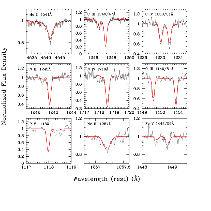
Figure 8.— The line-profiles of the selected lines observed in the FUSE and COS spectra (black lines) and the synthesized spectrum calculated using the TLUSTY model (red lines). The wavelength is shifted to the wavelength in vacuum.

Table 12The central star properties determined using the TLUSTY model.

Parameters	Values
Basic Parameters
$T_{\rm eff}$	36 360$\pm$700 K
$\log$ $g$	3.96$\pm$0.02 cm s-2
Photosphere Abundances ($\log$(H) = 12)
He/H ([He/H])	11.05$\pm$0.02 (+0.12$\pm$0.02)
C/H ([C/H])	9.38$\pm$0.02 (+0.99$\pm$0.04)
N/H ([N/H])	6.53$\pm$0.10 (–1.30$\pm$0.11)
O/H ([O/H])	8.36$\pm$0.10 (–0.33$\pm$0.11)
Ne/H ([Ne/H])	8.21$\pm$0.10 (+0.34$\pm$0.14)
P/H ([P/H])	3.64$\pm$0.10 (–1.82$\pm$0.11)
Fe/H ([Fe/H])	5.23$\pm$0.10 (–2.24$\pm$0.10)

The resulting spectrum synthesized using the TLUSTY and the observed FUSE and HST/COS spectra are shown in Fig. 8. The parameters, including the elemental abundances, are listed in Table 12. The derived stellar abundances are also listed in Table 11 for comparison. We were unable to detect any F absorption lines, e.g., F v $\lambda$ 1082/87/88 Å due to the low S/N ratio. The detection of the single isotope ³¹P is interesting because phosphorus (along with fluorine) is an $n$-capture element that is synthesized in the He-rich intershell during the TP-AGB phase.

We found that the stellar C and O abundances were close to the nebular RL abundances; however, the stellar He and Ne abundances were larger than the nebular abundances. The stellar N and Fe abundances were comparable to the nebular abundances. We may expect slightly higher stellar C, O, and Ne abundances than the nebular abundances, as the former are indicative of more recent products of AGB nucleosynthesis. These three elements are synthesized in the He-rich intershell during the AGB phase, and are then brought up to the stellar surface via the TDU. Note that the stellar C/O and the Ne/O ratios (10.75$\pm$2.43 and 0.75$\pm$0.23, respectively) are in good agreement with nebular ratios C/O (17.46$\pm$7.07 in RL and 6.83$\pm$3.63 in CEL) and Ne/O (0.51$\pm$0.06) in CEL. Although it is difficult to determine whether the RL or CEL abundance represents the nebular C and O chemical abundances in K648, the similarity of the C/O ratios determined from the RLs and CELs indicates a positive correlation with the stellar abundance.

K648 shows large stellar and nebular CEL [O/Fe] abundances (1.91$\pm$0.15 dex versus 1.49$\pm$0.13 dex). The [Ne/Fe] abundances were also large (2.01$\pm$0.16 dex in the CEL and 2.58$\pm$0.18 dex in the stellar region). It has been reported that metal-poor stars in the Milky Way exhibit large [$\alpha$/Fe] abundances, where the $\alpha$-elements include O, Ne, Mg, Si, and Ca. The effect is greatest for the most metal-poor populations, such as members of the stellar halo and, in particular, in the [O/Fe] (see, for example, McWilliam, 1997; Feltzing & Chiba, 2013). This is interpreted as a consequence of time delay in Fe production from Type Ia SNe relative to the $\alpha$-elements from core-collapse SNe. The $\alpha$-elements are mainly produced by Type II SNe. Both types of SNe should produce Fe in the proportions of $\sim$1/3 for Type II and $\sim$2/3 for Type Ia SNe. For M15, Sobeck et al. (2011) reported that three red giant branch (RGB) stars ($\langle$[Fe/H]$\rangle$ = –2.55), exhibited O abundance of 6.75-7.03 and the [O/Fe] of +0.62 to +0.85 ($\langle$[O/Fe]$\rangle$ = +0.75). If we observe an RGB star with [Fe/H] = –2.3, [O/Fe] should be +0.50, which corresponds to an O abundance of 6.89.

The difference between the [O/Fe] of M15 RGB stars reported by Sobeck et al. (2011) and that of K648 suggests that, in K648, O synthesis was $\gtrsim$0.9 dex during the TP-AGB phase. The TP-AGB phase nucleosynthesis process can contribute to enhancement of O and Ne abundances in the helium convective zone with ¹³C formed from mixed protons as an $n$-source using a nuclear network from H through S. The abundance of ¹⁶O may increase in proportion to the square root of the amount of mixed ¹³C until it reaches a significant fraction of ¹²C, whereas the abundance of ²²Ne may increase in proportion to the amount of mixed ¹³C, and attains half of the mixed ¹³C (Nishimura et al., 2009). Indeed, Lugaro et al. (2012) demonstrated that [Fe/H] = –2.19 AGB stars can synthesize significant quantities of O and Ne (see Section 4.1).

3.2.3 The core-mass of the CSPN

The core-mass of the CSPN can impose a significant constraint on the initial mass of the progenitor. Through construction of a TLUSTY model atmosphere, we obtained the $H_{\lambda}$ spectrum of the stellar photosphere. Using the $H_{\lambda}$ and the observed HST/WFPC2 F547M flux density $I_{\lambda}$ listed in Table 1, we determined the core-mass of the CSPN $M_{c}$ using Equation (1) of Shipman (1979), i.e.,

$$I_{\lambda} = 4\,\pi\,H_{\lambda}\,R^{2}\,D^{-2},$$ (3)

$$g = G\,M_{c}\,R^{-2},$$ (4)

where $R$ is the radius of the CSPN, $D$ is the distance to K648 from us, $g$ is the surface gravity of the CSPN, and $G$ is the gravitational constant.

Using the synthesized spectrum from TLUSTY model atmosphere fitting, we found that $H_{\lambda}$ = 4.53(+7) erg s^-1 cm^-2 Å^-1 at $\lambda$ 5483.88 Å by taking the transmission curve of the HST WFPC2/F547M band into account. Recent measurements of the distance to M15 have been reported by Reid (1996, 12.3$\pm$0.6 kpc), McNamara et al. (2004, 9.98$\pm$0.47 kpc), and van den Bosch et al. (2006, 10.3$\pm$0.4 kpc). We find $\log$ $g$ = 3.96$\pm$0.02 cm s^-2, as determined in Section 3.2.1.

If we use the average distance amongst these distance measurements, i.e., 10.9$\pm$0.5 kpc. we obtain $M_{c}$ = 0.68$\pm$0.07 $M_{\odot}$ and $R$ = 1.43$\pm$0.08 $R_{\odot}$ using Equations (3) and (4). Using the most recent data, i.e., $D$ = 10.3$\pm$0.4 kpc, the values of $M_{c}$ and $R$ are $M_{c}$ = 0.61$\pm$0.06 $M_{\odot}$ and 1.35$\pm$0.08 $R_{\odot}$, which are in agreement with Bianchi et al. (2001) and Rauch et al. (2002). We found that $R$ = 1.3 $R_{\odot}$ and $M_{c}$ of 0.62$\pm$0.10 $M_{\odot}$ with $D$ = 10.3 kpc and $\log$ $g$ = 4.0 cm s^-2. Rauch et al. (2002) calculated $M_{c}$ = 0.57 $M_{\odot}$ from the theoretical $T_{\rm eff}$-$\log$ $g$ diagram. The exact value of the $M_{c}$ is still dependent on the choice of distance. We will discuss the initial mass of K648 in section 4.1.

3.3. Dust features in the Spitzer/IRS spectrum

As discussed in Section 2.7, K648 exhibits the 6-9 $\mu$m PAH band, the 11.3 $\mu$m PAH band, and the broad 11 $\mu$m feature. These PAH bands are sometimes seen in C-rich PNe, such as BD+30^∘ 3639 (C/O = 1.59, Bernard-Salas et al., 2003; Waters et al., 1998), as well as O-rich PNe such as NGC6302 (C/O = 0.43, Wright et al., 2011; Molster et al., 2001). Both BD+30^∘ 3639 and NGC6302 exhibit strong crystalline silicate features at 23.5, 27.5, and 33.8 $\mu$m, which have never been observed in K648. In addition, the 9 and 18 $\mu$m features attributed to the amorphous silicate were also not seen in K648. Therefore, we concluded that K648 is a C-rich gas-and-dust PN.

Figure 9 shows the 5-15 $\mu$m spectrum, where the local dust continuum was subtracted by fourth-order spline fitting, using the same technique as applied for C-rich PNe by Otsuka et al. (2014). The flux density was then normalized to the intensity of the 8.6 $\mu$m PAH band. For comparison, we also show the Spitzer/IRS spectra of the C-rich halo PNe H4-1 (Tajitsu & Otsuka, 2014), as well as that of BoBn1 (Otsuka et al., 2010). We discuss the dust features in more detail below.

3.3.1 The 6-9 $\mu$m and 11.3 $\mu$m PAH bands

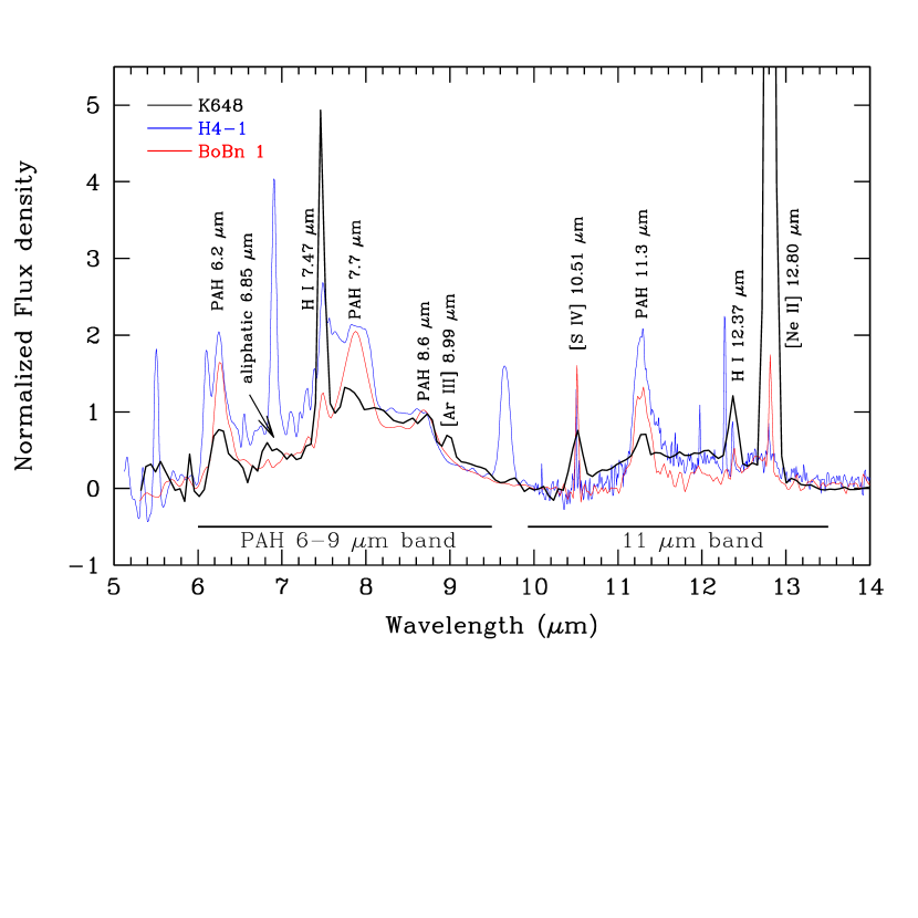
Figure 9.— The 5-15 $\mu$m spectra of C-rich halo PNe K648 (black), H4-1 (blue, from Tajitsu & Otsuka 2014), and BoBn1 (red, from Otsuka et al. 2010). The local continuum was subtracted from the observed flux, which was then normalized to that at 8.6 $\mu$m. The data for K648 are obtained from from the SL module. The 5-10 $\mu$m spectra of H4-1 and BoBn1 were obtained from the SL module and the remaining data from the SH module.

Table 13The results of Gaussian fittings to the PAH bands, the possible 6.85 $\mu$m aliphatic feature, and the broad 11 $\mu$m band.

$\lambda_{c}$	FWHM	$F$($\lambda$)	$I$($\lambda$)
($\mu$m)	($\mu$m)	(erg s-1 cm-2)	[$I$(H$\beta$) = 100]
6.25$\pm$0.01	0.22$\pm$0.02	2.25(–14)$\pm$1.88(–15)	2.20$\pm$0.21
6.47$\pm$0.01a	0.13$\pm$0.03	4.24(–15)$\pm$9.82(–16)	0.41$\pm$0.10
6.85$\pm$0.02b	0.21$\pm$0.04	6.01(–15)$\pm$1.65(–15)	0.59$\pm$0.16
7.83$\pm$0.01	0.25$\pm$0.03	1.34(–14)$\pm$2.12(–15)	1.31$\pm$0.22
			2.17$\pm$0.13d
8.73$\pm$0.01	0.16$\pm$0.04	5.37(–15)$\pm$1.55(–15)	0.53$\pm$0.15
11.31$\pm$0.01	0.25$\pm$0.01	1.00(–14)$\pm$6.46(–16)	0.98$\pm$0.08
11.81$\pm$0.03c	1.97$\pm$0.14	1.23(–13)$\pm$1.09(–14)	12.10$\pm$1.21

The 6-9 $\mu$m and 11.3 $\mu$m PAH band profiles are remarkably similar to those of H4-1 and BoBn1, although the intensity peak of the 7.7 $\mu$m PAH in K648 is smaller than those of BoBn1 and H4-1, which is attributed to noise around 7.7 $\mu$m.

We measured the central wavelength $\lambda_{c}$, FWHM, flux $F(\lambda)$, and relative intensity $I(\lambda)$ of each PAH band by single Gaussian fitting, and the results are shown in Table 13. For the 6.2 $\mu$m band, we employed a double Gaussian component fit, where one component corresponds to the 6.25 $\mu$m PAH band and the other to the He i $\lambda$ 6.47 $\mu$m.

Peeters et al. (2002) examined the profiles of the 6.2, 7.7, and 8.6 $\mu$m PAH bands using ISO/SWS spectra, and classified the spectra into Classes A, B, and C according to the peak positions of each PAH feature. Class B PAHs are frequently seen in C-rich PNe, including BoBn1 and H4-1, and have a peak in the range 6.235-6.28 $\mu$m, a stronger component at $\sim$7.8 $\mu$m than at 7.6 $\mu$m, and a peak at $>$8.62 $\mu$m. The 6.2, 7.7, and 8.6 $\mu$m features in K648 satisfy the definition of a Class B PAH spectrum.

According to the classification of the 11.3 $\mu$m PAH profiles by van Diedenhoven et al. (2004), the 11.3 $\mu$m PAH in K648 falls under Class B_11.2, with a peak at $\sim$11.25 $\mu$m. Many C-rich PNe in the Magellanic Clouds also have this class of PAH (Bernard-Salas et al., 2009).

3.3.2 The 6.85 $\mu$m aliphatic feature?

K648 exhibits a weak broad feature at 6.85 $\mu$m, which might be a combination of the 6.85 $\mu$m aliphatic feature (CH_2,3 asymmetric deformation) and [Ar ii] $\lambda$ 6.99 $\mu$m. Otsuka et al. (2014) established a relationship between $T_{\rm eff}$ and the $I$([Ar iii] $\lambda$ 8.99 $\mu$m)/$I$([Ar ii] $\lambda$ 6.99 $\mu$m) ratio in C-rich PNe based on P-I models with Cloudy code. Using their Equation (A1) and $T_{\rm eff}$ = 37 100 K (see Section 3.2), we found that the 6.85 $\mu$m aliphatic feature and the [Ar ii] $\lambda$ 6.99 $\mu$m intensities are 0.37$\pm$0.09 and 0.21$\pm$0.13, respectively, where the H$\beta$ intensity is 100.

Following Li & Draine (2012), we estimated the number ratio of C-atoms in aliphatic form relative to those in aromatic form using the 6-9 $\mu$m PAH band, i.e., $N_{\rm C,aliph}$/$N_{\rm C,arom}$. As we underestimated the 7.7 $\mu$m PAH flux in K648, we extrapolated a 7.7 $\mu$m PAH intensity of 2.17$\pm$0.13 using the PAH $I$(7.7 $\mu$m)/$I$(8.6 $\mu$m) ratio of 4.11$\pm$0.13 measured in BoBn1. Our derivation is $N_{\rm C,aliph}$/$N_{\rm C,arom}$ of $\sim$0.1-0.4, indicating that $<$29% of the C-atoms exists in aliphatic form in K648.

For a more accurate estimate of the number of C-atoms in the aliphatic form, $L$-band spectroscopy is useful to check for the existence of the 3.4 $\mu$m aliphatic feature, as well as $I$(3.3 $\mu$m PAH)/$I$(3.4 $\mu$m aliphatic).

3.3.3 The broad 11 $\mu$m band

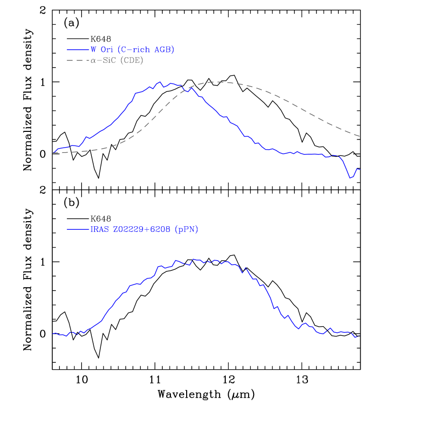
Figure 10.— The broad 11 $\mu$m band profiles. The 11.3 $\mu$m PAH and the atomic lines were subtracted out via Gaussian fitting in both (a) and (b). The flux density is shown normalized to the intensity peak. The spectral resolution of the C-rich AGB star W Ori and the proto PN IRAS Z02229+6208 was adjusted to match that of K648.

K648 exhibits the broad 11 $\mu$m feature, which is frequently seen in Galactic and Magellanic C-rich PNe (e.g., Otsuka et al., 2014; Bernard-Salas et al., 2009; Stanghellini et al., 2012). The band profile appears to show an almost flat portion in the range 11.4-12.2 $\mu$m. However, as shown in Fig. 10(a), the resulting band profile did not exhibit a flat top after removal of the 11.3 $\mu$m PAH band and the atomic lines.

The results of Gaussian fitting are also listed in Table 13. The FWHM of the 11 $\mu$m band is comparable to those for H4-1 (2.08$\pm$0.05 $\mu$m) and BoBn1 (1.85$\pm$0.39 $\mu$m); however, $\lambda_{c}$ was slightly blue-shifted (12.28$\pm$0.06 $\mu$m in H4-1 and 12.30$\pm$0.08 $\mu$m in BoBn1). Our results corroborate those of Bernard-Salas et al. (2009), who reported that the profile and the central wavelength of the 11 $\mu$m band in MC PNe differ from source to source.

There is some debate regarding the origin of the broad 11 $\mu$m feature. Silicon carbide (SiC) is one possible explanation for the feature at 11 $\mu$m in C-rich MC PNe (Bernard-Salas et al., 2009). In Fig. 10(a), as a SiC template, we show a comparison with the 11 $\mu$m band profile of the Galactic solar metallicity C-rich AGB star W Ori, extracted from the archive ISO/SWS spectrum. These data were downloaded from Sloan et al. (2003). Abia et al. (2002) reported a C/O ratio of 1.005, and a metallicity of [M/H] = +0.05. The $\lambda_{c}$ (11.2 $\mu$m) and FWHM (1.51 $\mu$m) in the 11 $\mu$m band of W Ori differ significantly from those measured for K648. The 11 $\mu$m band profile in W Ori may be fitted to an absorption efficiency $Q_{\lambda}$ of a spherical $\alpha$-SiC grain (or 6-H SiC, hexagonal unit cell) calculated from Pegourie (1988), which peaks sharply at $\sim$11.2 $\mu$m and has an FWHM of $\sim$1.2 $\mu$m. However, we must be careful with $\lambda_{c}$ in W Ori. Leisenring et al. (2008) demonstrated how the C₂H₂ absorption band around 13.7 $\mu$m, as well as the SiC self-absorption band around 10 $\mu$m affect the central wavelength of SiC in AGB stars such as W Ori. They argued that the C₂H₂ absorption band suppressed the long-wavelength part of the feature at 11 $\mu$m, and caused the central wavelength to be blue-shifted. This may be the case for W Ori. We could fit neither $\lambda_{c}$ nor the FWHM of the 11 $\mu$m band, even with a continuous distribution of ellipsoids (CDE, e.g., Bohren & Huffman, 1983; Min et al., 2003) of $\alpha$-SiC; we find $\lambda_{c}\sim 11.8\mu$m and a FWHM of $\sim$2 $\mu$m using the $Q_{\lambda}$ for the CDE $\alpha$-SiC, as shown by the by the gray line in Fig. 10(a).

Kwok et al. (2001) argued that a collection of out-of-plane bending modes of aliphatic side groups attached to an aromatic ring could result in to the broad 11 $\mu$m feature. Indeed, we found the feature at 6.85 $\mu$m in K648, corresponding to possibly aliphatic C. Figure 10(b) shows a comparison of the 11 $\mu$m band profiles of K648 and the proto-PN IRAS Z02229+6208. The [C/H] and [M/H] abundances of this proto-PN are +0.29 and –0.50, respectively, (Reddy et al., 1999). The measured values of $\lambda_{c}$ and the FWHM of IRAS Z02229+6208 are 11.68$\pm$0.02 $\mu$m and 1.81$\pm$0.05 $\mu$m, respectively. The 11 $\mu$m band profile in IRAS Z02229+6208 exhibits a good fit to that of K648, except for the $\lesssim$11 $\mu$m part of the 11 $\mu$m band. According to Kwok et al. (2001), K648 may have a few cyclic alkanes, which contribute to the 9.5-11.5 $\mu$m part of this band (see Fig. 4 of Kwok et al., 2001).

The low metallicity of K648 implies a very low abundance of Si. Indeed, we did not detect any lines corresponding to Si in either the nebula or the central star. Therefore, we expect that the broad 11 $\mu$m band profile in K648 is attributable to a wide variety of alkane and alkene groups attached to hydrogenated aromatic rings, rather than to SiC.

3.4. Radiative transfer modeling and SED fitting

We constructed an SED model to investigate the physical conditions of the gas and dust grains and derive their masses using Cloudy c10.00. The quantity of dust mass formed in extremely metal-poor objects such as K648 is of interest. The gas mass as well as the core-mass of the CSPN are required to unveil the origin and evolution of K648 via a comparison of these parameter values with the results of AGB nucleosynthesis models.

3.4.1 Modeling approach

Figure 11.— The SED of the CSPN of K648 synthesized using TLUSTY. This SED was adopted in the dust+gas SED model using Cloudy code as the incident SED.

Figure 12.— The hydrogen density radial profile used in the Cloudy P-I SED modeling.

We attempted to fit the observed SED in the range 0.1-160 $\mu$m, assuming that the dust in K648 is composed of PAH molecules and amorphous carbon (AC) grains. No SiC grains were considered to fit the broad 11 $\mu$m feature.

The distance to K648 is required to compare our model values with the observed fluxes; here we assumed a distance of 10.9 kpc. For the incident SED from the central star, we used the synthesized spectrum of the central star of K648 using the TLUSTY model, as discussed in Section 3.2. The input SED is shown in Fig. 11. We adjusted the input SED to match the de-reddened absolute $V$-band magnitude of –0.528 measured from HST/F547M photometry of the CSPN. The number of Lyman continuum photons $N_{\rm Lyc}$ with $>$13.5 eV was 6.92(+45) s^-1, as determined from the synthesized spectrum of the CSPN.

The P-I model construction with the Cloudy and other codes involves an ad hoc nebular geometry and central stellar property modification. Until it gives a right prediction to the line intensities and continuum, one must adjust not only the chemical abundances but also the model nebular geometry with a new value close to the observation indication. In order to tune the other diagnostically indicated physical properties, e.g., electron temperature, one even needs to consider other chemical elements which were not observed at all. We employed the observed values of the gas-phase elemental abundances listed in Table 10 as initial estimates, and refined these to match the observed line intensities of each element. We considered the RL and CEL C line fluxes and the observed CEL O line fluxes to determine the nebular C and O abundances, respectively. We revised the transition probabilities and collisional impacts of C iii], [N ii], [O ii, iii], [F ii,iv], [Ne ii,iii,iv], [S ii,iii], [Cl ii,iii] and [Ar ii,iii,iv], which were the same as those used in our semi-empirical ICF abundance calculations (i.e., using IP coincidence method). The abundances of other elements were fixed to be constant, with [X/H] = –2.3.

We determined the radial hydrogen density profile of the nebula based on the radial intensity profile of the HST/WFPC2 F656N image using Abel transformation, and assuming spherical symmetry. We fixed the outer radius to $R_{\rm out}=2.1^{\prime\prime}$ (0.11 pc) and the inner radius to $R_{\rm in}=0.14^{\prime\prime}$ (0.0072 pc). We used a constant filling factor of $\epsilon=0.5$. The hydrogen density radial profile is shown in Fig. 12. The $R_{\rm out}$ that was used corresponds to the Strömgren radius (0.11 pc), assuming $T_{\epsilon}$ = 10⁴ K, $n({\rm H^{+}})$ = $n_{\epsilon}$ = 3000 cm^-3, and the same values of $\epsilon$ and $N_{\rm Lyc}$

We assume that both PAH molecules and AC grains exist in the nebula, and that the observed IR-excess from MIR to FIR wavelengths is due to the thermal emission from these species. We assumed spherical AC grains and PAH molecules. The optical constants were taken from Draine & Li (2007) for PAHs and from Rouleau & Martin (1991) for the AC grains. For the PAHs, we assumed that the radius was in the range of 0.0004-0.0011 $\mu$m (i.e., 30-500 C atoms) with an $a^{-3.5}$ size distribution. For the AC grains, we used the standard interstellar dust grain size distribution reported by Mathis et al. (1977), i.e., an $a^{-3.5}$ size distribution, but with a smaller radius of 0.0005-0.010 $\mu$m, which was determined by running several test models.

To evaluate the degree of accuracy of the model fitting, we calculated the chi-square ($\chi^{2}$) value from the 39 gas emission fluxes, 10 gas-phase abundances, and the five broad band fluxes, as well as the 15 flux densities of the features of interest from UV to FIR wavelengths.

3.4.2 Modeling results and SED fitting

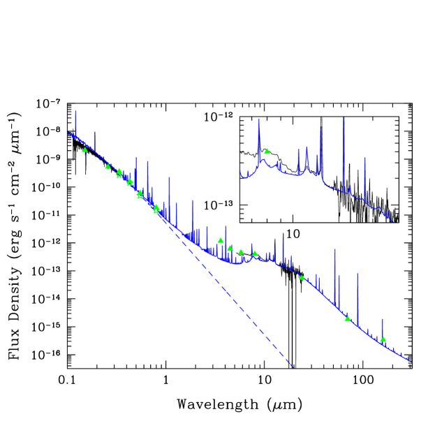
Figure 13.— The SED of K648. The blue solid and broken lines are the predicted SED of the sum of the CSPN and the nebula and the incident SED of the CSPN, respectively. The black lines are the observed spectra obtained from the HST/FOS and Spitzer/IRS. The Subaru/HDS spectrum is not shown because its appeared to be partially contaminated by foreground stars. Instead, we plotted the HST/WFPC2 photometry, indicated by the green asterisks (CSPN) and triangles (CSPN+PN). The green triangles in the MIR and FIR (3.6/4.5/5.8/8.0/24/70/100/160 $\mu$m) are Spitzer/IRCS/MIPS and Herschel/PACS photometry.

Table 14The properties from the Cloudy P-I model.

Parameters	Values
	Central Star
$M_{\rm V}$	–0.528, measured from HST/F547M obs
$L_{\ast}$	3076 $L_{\odot}$
$T_{\rm eff}$	36 360 K
$\log\,g$	3.96 cm s-2
Distance	10.9 kpc
	Nebula
Abundancesa	He:11.00, C:8.71, N:6.96, O:7.82,
($\log$$n$(X)/$n$(H)+12)	F:5.41, Ne:7.02, S:5.48, Cl:3.44
	Ar:4.44, Fe:5.48, Others:[X/H] = –2.3
Geometry	Spherical
Shell size	$R_{\rm in}$ = 0.14 ″ (0.0072 pc), $R_{\rm out}$ = 2.1 ″ (0.125 pc)
$n_{\rm H}$	See Fig. 12
filling factor	0.50
$\log I$(H$\beta$)	–11.972 erg s-1 cm-2 (de-redden)
$m_{\rm g}$	4.81(–2) $M_{\odot}$
	Dust in Nebula
Composition	PAHs, amorphous carbon (AC)
Grain size	0.0005-0.010 $\mu$m for AC
	0.0004-0.011 $\mu$m for PAH
$T_{d}$(PAHs)	140-472 K
$T_{d}$(AC)	99-290 K
$m_{d}$(Tot.)b	4.95(–7) $M_{\odot}$
$m_{d}$(Tot.)/$m_{\rm g}$	1.029(–5)

Table 15Comparison between the results of the P-I model and the observations.

Ion	$\lambda$	$I$(P-I)	$I$(Obs)	$\Delta$$I$/$I$(Obs)
	(Å/$\mu$m)	[$I$(H$\beta$) = 100]	[$I$(H$\beta$) = 100]	($\%$)
C iii$]$	1906/09	468.701	334.984	39.92
$[$C ii$]$	2323	25.134	17.091	47.06
[O ii]	3726	17.646	17.383	1.51
[O ii]	3729	9.385	9.387	0.02
[Ne iii]	3869	10.255	9.939	3.18
[Ne iii]	3968	3.091	3.147	1.78
C ii	4267	0.492	0.726	32.23
H$\gamma$	4340	46.974	46.674	0.64
[O iii]	4363	2.273	2.782	18.31
He i	4388	0.640	0.517	23.84
He i	4471	5.218	4.914	6.18
[F ii]	4791	0.105	0.110	4.94
[F ii]	4870	0.033	0.030	8.83
[Fe iii]	4881	0.054	0.051	4.92
He i	4922	1.383	1.290	7.23
[O iii]	4931	0.032	0.038	14.87
[O iii]	4959	79.089	74.974	5.49
[O iii]	5007	238.058	227.263	4.75
[Cl iii]	5518	0.022	0.021	3.14
[Cl iii]	5538	0.027	0.028	3.50
[N ii]	5755	0.064	0.052	22.17
He i	5876	15.676	14.834	5.67
[S iii]	6312	0.147	0.119	23.55
[N ii]	6548	0.979	0.901	8.70
H$\alpha$	6563	282.047	282.399	0.12
[N ii]	6584	2.890	3.180	9.12
He i	6678	4.182	4.114	1.65
[S ii]	6716	0.069	0.087	20.98
[S ii]	6731	0.110	0.133	17.23
[Ar iii]	7135	0.389	0.384	1.21
[O ii]	7323	1.573	1.792	12.20
[O ii]	7332	1.256	1.450	13.39
H i	7.47	3.192	3.150	1.35
[Ar iii]	9.00	0.296	0.324	8.64
[S iv]	10.51	1.095	1.064	2.95
[Ne iii]	15.55	8.736	11.545	24.33
[Ne ii]	12.80	3.645	14.980	75.67
[S iii]	18.71	2.343	1.332	75.93
[S iii]	33.47	0.893	0.612	45.89
IRS-1	8.55	13.365	15.859	15.73
IRS-2	9.825	4.809	4.560	5.46
IRS-3	12.03	4.973	4.531	9.75
IRS-4	14.00	2.672	2.322	15.08
IRS-5	25.50	9.044	9.136	1.01
Band	$\lambda$	$F_{\nu}$(P-I)	$F_{\nu}$(Obs)	$\Delta$$F_{\nu}$/$F_{\nu}$(Obs)
	(Å/$\mu$m)	(mJy)	(mJy)	($\%$)
F160BW	1515	26.647	15.993	66.61
F170W	1820	25.808	20.886	23.57
F255W	2599	15.952	11.907	33.97
F300W	2989	13.823	10.543	31.11
F336W	3360	12.211	13.393	8.82
F439W	4312	9.554	9.793	2.43
F547M	5484	5.810	6.025	3.56
F814W	7996	3.701	3.921	5.62
IRAC-1	3.51	1.273	5.096	75.01
IRAC-2	4.50	1.499	4.158	63.95
IRAC-3	5.63	2.035	5.046	59.67
IRAC-4	7.59	4.734	8.510	44.37
MIPS-1	23.21	11.300	10.684	5.77
PACS-B	68.93	3.207	2.950	8.71
PACS-R	153.9	1.804	2.680	32.69
${\chi}^{2}$				88.12

Note. — The data in the IRS-1, 2, 3, 4, and 5 bands are the integrated fluxes between the following wavelengths: 8.26-8.84 $\mu$m, 9.7-9.95 $\mu$m, 11.9-12.16 $\mu$m, 13.9-14.1 $\mu$m and 24.5-26.5 $\mu$m, respectively. Data are shown with two or three decimal places to avoid rounding errors.

Table 16Comparison of the observed elemental abundances and those predicted using the P-I model.

X	Obsa	P-Ib	$\triangle^{\rm c}$	ICF(XObs)d	ICF(XP-I)e
	log(X/H)+12	log(X/H)+12	log(XObs/XP-I)
He	11.02$\pm$0.03	10.99$\pm$0.20	+0.03$\pm$0.20	1.04$\pm$0.01	1.00
C	8.97$\pm$0.17	8.71$\pm$0.20	+0.26$\pm$0.26	1.33$\pm$0.24	1.00
N	6.36$\pm$0.10	6.96$\pm$0.20	–0.60$\pm$0.22	4.02$\pm$0.81	20.56
O	7.73$\pm$0.03	7.82$\pm$0.20	–0.09$\pm$0.20	1.00	1.00
F	5.42$\pm$0.11	5.41$\pm$0.20	+0.01$\pm$0.23	4.02$\pm$0.81	5.22
Ne	7.44$\pm$0.03	7.02$\pm$0.20	+0.42$\pm$0.20	1.00	1.00
S	5.40$\pm$0.07	5.48$\pm$0.20	–0.08$\pm$0.21	1.00	1.00
Cl	3.58$\pm$0.15	3.44$\pm$0.20	+0.14$\pm$0.25	1.19$\pm$0.29	1.05
Ar	4.60$\pm$0.13	4.44$\pm$0.20	+0.16$\pm$0.24	1.19$\pm$0.29	1.04
Fe	5.02$\pm$0.12	5.48$\pm$0.20	–0.46$\pm$0.23	4.02$\pm$0.81	5.15

Figure 13 shows the predicted SED, the observed spectra, and the band flux densities. The predictions were taken at the matter-bounded radius near the Strömgren edge (or at the radius close to the ionization-bounded radius of the P-I model nebula). This provides an appropriate level of nebular excitation, e.g., for O²⁺/(O⁺+O²⁺). Note that the observed and predicted nebular ratios O²⁺/(O⁺ + O²⁺)$\sim$0.75 (0.92 in BoBn1 and 0.67 in H4-1, Otsuka et al., 2010; Otsuka & Tajitsu, 2013) were large despite the cool CSPN of K648. Such a high ratio indicates that K648 could be a matter-bounded nebula, where the edge of the mass distribution falls inside the Strömgren edge, rather than an ionization-bounded nebula, and also it might be related to the small nebula mass.

The fitted elemental abundances, gas mass $m_{g}$, dust mass $m_{d}$, and dust temperatures $T_{d}$ are listed in Table 14. The third and fourth columns of Table 15 show a comparison of the predicted fluxes and flux densities with the observed data. The discrepancies of each flux and each flux density between the observation and model are listed in the final column. In the SED fitting for the MIR wavelengths, we place emphasis on the band fluxes (IRS-1,2,3,4,5) and flux densities (IRAC-4 and MIPS-1) rather than the atomic line fluxes, because our interest in SED modeling is in calculating the gas and dust masses. Therefore, there are some discrepancies in the MIR atomic lines between the observed and calculated data. The $\chi^{2}$ values are listed in the bottom line of Table 14. The chi-square analysis implies that, within 1-$\sigma$, there was no difference between the predicted and the observed flux densities/band fluxes, but rather a slight (negligible) disagreement between the calculated and observed fluxes, owing to the C iii$]$ $\lambda\lambda$ 1906/09 Å flux. Without the C iii$]$ $\lambda\lambda$ 1906/09 Å flux, $\chi^{2}$ = 34.75 indicates that the modeled flux densities and band fluxes are in excellent agreement with the observations.

The discrepancy between the observed calculated C iii$]$ $\lambda\lambda$ 1906/09 Å line fluxes appears to result from fluctuations in the structure of $T_{\epsilon}$. The C iii$]$ lines are the most sensitive to the $T_{\epsilon}$ among those considered in the model; the excitation energy difference between the upper and the lower levels ($\chi$) is 6.5 eV and the excitation temperature is 75 380 K (=$\chi$/$k$, where $k$ is the Boltzmann constant). We used $T_{\epsilon}$ = 10 270 K in the calculations of C²⁺, whereas the volume-averaged $T_{\epsilon}$(C²⁺) in the model was 11 090 K. With a constant $n_{\epsilon}$, but a difference of only 820 K, the volume emissivity of this complex line at 11 090 K became $\sim$1.65 times larger than that with 10 270 K. Accordingly, we obtained C iii$]$ $\lambda\lambda$ 1906/09 Å fluxes that were greater than those of the observations by a factor of $\sim$1.65. The H$\beta$ emissivity at $T_{\epsilon}$ = 10 270 K was 1.07 times greater than that at $T_{\epsilon}$ = 11 090 K. Therefore, the modeled C²⁺ abundance was smaller than the observation by $\sim$–0.10 dex. Taking the differences in the structure of $n_{\epsilon}$ and $T_{\epsilon}$ between the model and the observed data into account, we estimate that the accuracy of the elemental abundances calculated using the was within $\sim$0.2 dex.

As the model provides decent predictions for the [S iii] $\lambda\lambda$ 18.7/33.5 $\mu$m, [S iii] $\lambda$9532 Å ($I$(P-I)) of [S iii] $\lambda$9532 Å = 5.760, which are not listed in Table 15), and [S iii] $\lambda$ 6312 Å simultaneously, we may assume that the two MIR [S iii] lines are not spurious, but rather genuine features of the spectra.

Our P-I model with the Cloudy code was not able to fit [Ne ii] $\lambda$ 12.80 $\mu$m, whereas the prediction of the other atomic lines of similar IPs, i.e., ions such as [F ii] (see below), [S iii], [Ar iii], and [Cl iii], is in good agreement with the observations. Many P-I models using Cloudy have been used to fit the [Ne ii] $\lambda$ 12.80 $\mu$m in PNe; however, to our knowledge, there has been little success (e.g., Pottasch et al., 2011, 2009). In our model, we monitored the chi-square values to obtain the best fitting parameters. With an almost constant radial density profile, the [Ne ii] $\lambda$ 12.80 $\mu$m could be modeled; however, the other line-fluxes and band fluxes/flux densities exceeded the observed values, i.e., chi-square increased. The recombination rates for some heavy element ions (e.g., S⁺) are uncertain, so that photo-ionization models may give line fluxes that are in poor agreement with measured data. Therefore, the lack of agreement may be due to the uncertainties in the atomic data for Ne⁺. Improvements in these data, however, are beyond the scope of this paper.

Our P-I model predictions provide good fits to two of the [F ii] line intensities. If both lines are not [F ii] lines but other elemental lines, the P-I model cannot fit these two lines simultaneously. Therefore, we conclude that the detected [F ii] lines are likely to be real. The two observed [F ii] line fluxes and the calculated elemental abundance of F using the ICF(F) are in good agreement with the predictions of the model.

The second and third columns of Table 16 list a comparison of the nebular elemental abundances determine using the semi-empirical ICF method and the P-I model. As we mentioned above, the accuracy of the elemental abundances determined using the P-I model was within $\sim$0.2 dex. Careful treatment for the Ne abundance is necessary for the reasons discussed above. Therefore, we excluded the Ne abundance from the following discussion. The difference between the two data sets, ($\triangle$), is listed in the fourth column of Table 16. The agreement between the He, C, O, F, S, Cl, and Ar abundances between the ICF method and the P-I model is generally good.

However, poor agreement is found for N and Fe ($|\triangle|$$\geq$0.2 dex). The final two columns of Table 16 list the ICF values used in Section 3.1.5 and those predicted by the P-I model. The ICF values from the P-I model were generally in agreement with those of the semi-empirical methods, except for N. This is because most fractional ionizations occurred in other ionic stages: the P-I prediction suggests 5$\%$ for N⁺ and 95 $\%$ for N²⁺. Poor agreement for N between the ICF and P-I models is often found for PNe and in the O-rich halo PN DdDm1 (see e.g., Otsuka et al., 2009; Delgado-Inglada et al., 2014). In many cases, including DdDm1, N⁺ abundances determined from optical spectra alone have been used to determine the elemental N abundance, because it is difficult to detect the N²⁺ forbidden lines, which appear in the UV or FIR spectra. Based on grid models using Cloudy, Delgado-Inglada et al. (2014) proposed that the N/O ratio for PNe showing no-He ii lines can be estimated by the following equations,

$${\rm\frac{N}{O}} = {\rm ICF(N)_{GI14}\cdot\frac{N^{+}}{O^{+}}},$$ (5)

$${\rm ICF(N)_{GI14}} = {\rm 10^{0.64\cdot\frac{O^{2+}}{O^{+}+O^{2+}}}.}$$ (6)

In the case of K648, the ICF(N)_GI14 and the N/H abundance using the observed O^+,2+, N⁺ abundances (Table 7) and the elemental O abundance (Table 10) were estimated to be 3.40$\pm$2.42 and 7.77(–6)$\pm$5.82(–6). The $\log_{10}$(N/H)+12 of 6.89$\pm$0.33 is very close to the model predicted value (6.96$\pm$0.20), although we should note that the ionic and elemental abundances would depend on the density structure, incident ionization source, ionization boundary condition, gas metallicity, dust grains/molecules, and so on. We should keep in our mind that we were unable to detect N iii$]$ $\lambda$1750 Å in K648. The predicted line-intensity around 1750 Å FOS spectrum with S/N = 1 was $\sim$5.3 (i.e., a detection limit), which is approximately three times larger than the prediction of the P-I model (i.e., 1.7). The N iii$]$ $\lambda$ 1750 Å line was too faint to detect using FOS. As the P-I model provided a value of ICF(N) that was too large, in this paper we prefer to use the semi-empirically determined N abundance, i.e., the ICF abundance (not ICF(N)_GI14). The P-I model indicates that Fe ions are also concentrated in other ionic stages, rather than the observed ionic stage, i.e., 20% Fe²⁺ and 80% Fe³⁺. The availability of the N²⁺ and Fe³⁺ lines would be expected to improve the accuracy of the abundance calculation. FIR observations using SPICA/SAFARI would be helpful to detect [N ii] $\lambda$ 121.3 $\mu$m and $[$N iii$]$ $\lambda$57.3 $\mu$m lines and verify ICF(N) in PNe.

Note that we used the ICF abundances rather than the P-I results. Analysis with the P-I results, however, is not expected to alter the conclusions. The P-I results should be carefully examined in a more sophisticated future study.

The nebula is fully ionized, so that the ionized gas mass is consistent with $m_{g}$. Bianchi et al. (1995) determined an ionized gas mass of 0.05-0.09 $M_{\odot}$, and Kingsburgh & Barlow (1992) determined it to be 0.042 $M_{\odot}$. Both authors assumed a constant density profile. Although $m_{g}$ (and $m_{d}$) depends on the distance used, $m_{g}$ in this work is consistent with these estimates.

Here, we estimate $m_{d}$ and the dust-to-gas mass ratio $m_{d}$/$m_{g}$. If we assume that the AC dust grains have a radius of 0.0005-0.25 $\mu$m and a size distribution that follows $a^{-3.5}$, we obtain $m_{d}$ = 9.74(–7) $M_{\odot}$ and $m_{d}$/$m_{g}$ = 2.07(–5). However, this model does not fit the flux density at the above-mentioned wavelengths. To our knowledge, the value of $m_{d}$ = 4.95(–7) $M_{\odot}$ for K648 is the smallest mass among known PNe, and is approximately one order of magnitude smaller than that of BoBn1, where the $m_{d}$ = 5.78(–6) $M_{\odot}$. For BoBn1, Otsuka et al. (2010) used grains with a radius of 0.001-0.25 $\mu$m with an $a^{-3.5}$ size distribution in the SED model, whereas for K648 we used much smaller grains to match the observed SED at wavelengths in the range 10-15 $\mu$m. We found the ratio $m_{d}$/$m_{g}$ = 1.03(–5), which was much lower than that for BoBn1 (5.84$\times$10^-5). For H4-1, Tajitsu & Otsuka (2014) reported that $m_{g}$ = 0.3 $M_{\odot}$, $m_{d}$ = 7.34(–4) $M_{\odot}$, and $m_{d}$/$m_{g}$ = 2.48(–3); however, H4-1 contains abundant cold dust and hydrogen-rich molecules. Among these C-rich halo PNe, where the metallicity is similar to that of K648, we could not find dependence of the metallicity on the dust mass.

3.5. Expansion velocities and the time since the AGB phase

Table 17Expansion velocities of K648.

Ion	Type of	I.P.	Num. of	$\langle{V_{\rm exp}}\rangle$
	lines	(eV)	sample lines	(km s-1)
[O i]	CEL	0.00	2	10.12$\pm$0.27
[S ii]	CEL	10.36	2	14.70$\pm$0.28
H i	RL	13.59	26	15.07$\pm$0.58
[O ii]	CEL	13.62	2	15.99$\pm$0.18
[N ii]	CEL	14.53	3	13.81$\pm$0.43
[Fe iii]	CEL	16.18	2	12.70$\pm$1.05
[F ii]	CEL	17.42	2	13.85$\pm$0.90
[S iii]	CEL	23.33	1	15.96$\pm$0.57
[Cl iii]	CEL	23.81	2	16.12$\pm$1.55
C ii	RL	24.38	6	19.37$\pm$0.99
He i	RL	24.59	17	15.71$\pm$0.56
[Ar iii]	CEL	27.63	1	14.25$\pm$0.16
N ii	RL	29.60	2	15.72$\pm$1.49
[O iii]	CEL	35.12	4	15.75$\pm$0.52
O ii	RL	35.12	1	12.65$\pm$0.99
[Ne iii]	CEL	40.96	2	13.75$\pm$0.09
C iii	RL	47.89	3	15.54$\pm$0.63

Note. — The third and fourth columns list the IP and the number of sample lines used in the calculation of the average $V_{\rm exp}$ of each ion, respectively.

We employed a multiple Gaussian fitting method for the flux measurements, except for the strong lines [O ii] $\lambda\lambda$ 3726/29 Å, [O iii] $\lambda\lambda$ 4959/5007 Å, [O i] $\lambda$ 6300 Å, H$\alpha$, and [N ii] $\lambda$ 6583 Å, because these lines have a weak broad tail component or a small offset velocity component. Here, we focus on the nebula expansion velocity $V_{\rm exp}$ determined from the main Gaussian component of each line.

We measured $V_{\rm exp}$ using the following relation:

$$V_{\rm exp}=1/2~{}(V_{\rm FWHM}^{2}-V_{\rm therm}^{2}-V_{\rm instr}^{2})^{1/2},$$ (7)

where $V_{\rm FWHM}$ is the FWHM of the velocity, $V_{\rm therm}$ is the thermal broadening velocity, and $V_{\rm instr}$ is the instrumental velocity (e.g., Otsuka et al., 2010, 2009; Bianchi et al., 2001). Here, $V_{\rm therm}$ is represented by 21.4$(T_{\epsilon}{\times}10^{-4}/A_{r})^{1/2}$, where $A_{r}$ is the relative atomic mass of the target ion. For CELs, we used the $T_{\epsilon}$ listed in Table 6. For RLs, we used $T_{\epsilon}$(BJ) for H i, C ii,iii, [N ii], and O ii and the $T_{\epsilon}$(He i) = 6710 K for the He i lines. We measured $V_{\rm instr}$ for all the identified lines listed in Table A in the Appendix using the nearby Th-Ar lines, i.e., 4.3 km s^-1 for [Ar iii] $\lambda$ 7135 Å, He i $\lambda$ 7281 Å, and [O ii] $\lambda\lambda$ 7320/7330 Å (the resolving power of these lines was $\sim$69 000), and 8.8-9.0 km s^-1 for the others . We did not include the turbulent velocity, because these velocities have been measured in $\sim$100 Galactic PNe by e.g., Acker et al. (2002) and Gesicki et al. (2003), who found no turbulent velocities in PNe with non-WC type central stars, such as K648.

The resulting $V_{\rm exp}$ are summarized in Table 17. We measured the $V_{\rm exp}$ of over 100 lines selected from the lines listed in Appendix Table A. For each ion, we excluded the measurements far from the average using 1-$\sigma$ clipping. We then calculated the average expansion velocity, $\langle{V_{\rm exp}}\rangle$ of, the 18 ions listed in the final column of Table 17.

Our measurements showed good agreement with those of Bianchi et al. (2001), who measured the $\langle{V_{\rm exp}}\rangle$(H i) of 16.7 km s^-1 using H$\alpha$ and $\langle{V_{\rm exp}}\rangle$([N ii]) of 11.9 km s^-1, using both [N ii] $\lambda$ 6548 Å and [N ii] $\lambda$ 6583 Å lines, and with a constant electron temperature of $T_{\epsilon}$ = 10 000 K for the thermal broadening velocities. We used 26 H i lines for the $\langle{V_{\rm exp}}\rangle$(H i) and 3 lines for the $\langle{V_{\rm exp}}\rangle$([N ii]) calculations with $T_{\epsilon}$(BJ) and $T_{\epsilon}$([N ii]), respectively. The slight differences between our data and those reported by Bianchi et al. (2001) can be attributed to the value of $T_{\epsilon}$ used and the number of sample lines.

The correlation between the $\langle{V_{\rm exp}}\rangle$ and IPs is given by

$$\langle{V_{\rm exp}}\rangle=(5.23~{}\pm~{}4.03)\cdot 10^{-3}~{}{\rm IP}+13.54~{}\pm~{}1.01.$$ (8)

The correlation factor was 0.32. Assuming that K648 has a standard ionized structure, i.e., high-intensity IP lines are emitted from regions close to the central star and low-intensity IP lines are emitted from regions far from the central star, the expansion velocity of the nebula may be slowing with an almost constant value of $r$. In general, the PN shell is known to follow a Hubble type expansion, i.e., acceleration of the expanding gas shell. Perhaps it did not gain its impulsion from the CSPN yet.

As we found for BoBn1 (Otsuka et al., 2010), $V_{\rm exp}$ for [O ii] was at least 1.5 km s^-1 smaller than that for [O iii].

The apparent outer radius of K648 is 2.1^′′, which corresponds to 0.125 pc at 10.9 kpc. The wind velocity of K648 during the AGB mass-loss phase is unknown. We used an expansion velocity of $\langle{V_{\rm exp}}\rangle$(H i) = 15.07 km s^-1, and estimated the dynamical age of the K648 nebula to be 8110$\pm$490 years since the AGB phase. Rauch et al. (2002) estimated the post-AGB age of 6800${}^{+3500}_{-2000}$ yrs by plotting their derived luminosity and surface gravity on theoretical evolutional tracks. However, the evolutionary age after the AGB phase with more precision is unknown at this moment. McCarthy et al. (1990) investigated the disagreement between evolutionary and dynamical time scales for the evolution of the CSPNe using the results of high resolution spectra of about 23 CSPNe. According to them, the AGB-CSPN evolutionary transition times could have been increased by small additional amounts of residual envelope material remaining after the superwind mass-loss phase.

4. Discussion

4.1. Comparison with the AGB nucleosynthesis model

Table 18 Comparison of the observed nebular abundances with the predictions of the [Fe/H] = –2.19 AGB model.

	Models						Obs
	Initial mass ($M_{\odot}$)	0.9	0.9	1.25	1.25	1.5
Elements	PMZ mass ($M_{\odot}$)	0	2(–3)	0	2(–3)	0
He		11.00	11.00	11.00	11.00	11.01	11.02$\pm$0.03
C		9.07	9.04	8.94	8.90	9.26	8.97$\pm$0.17
N		7.55	7.53	6.67	6.68	6.76	6.36$\pm$0.10
O		7.48	7.63	7.31	7.47	7.56	7.73$\pm$0.03
F		4.74	5.03	4.35	4.78	5.08	5.42$\pm$0.11
Ne		7.33	7.87	6.95	7.65	7.68	7.44$\pm$0.03
Pa		3.48	3.64	3.36	3.54	3.49	3.64$\pm$0.10
ejected mass during		2.0(–3)	2.0(–3)	8.0(–3)	8.0(–3)	5.99(–1)	4.8(–2)b
last TP ($M_{\odot}$)
core-mass ($M_{\odot}$)		0.77	0.77	0.66	0.66	0.66	0.61-0.63
envelope mass ($M_{\odot}$)		0.04	0.04	0.02	0.03	0.18	$\cdots$

Note. — The initial He, C, N, O, F, Ne and P abundances in all models are 10.92, 6.29, 5.69, 6.55, 2.24, 5.79 and 3.23, respectively.

In Section 3.2.3, we determined the core-mass of the central star as 0.61-0.68 $M_{\odot}$, depending on the choice of the distance to M15. The initial-final mass relation has been studied using solar metallicity for young ($\sim$1-2 Gyr) open clusters (e.g., Kalirai et al., 2008); however, it has been not studied using metal-poor old clusters. Semi-empirical initial-final mass relations are only available for the chemical composition of the solar neighborhood and for Magellanic Clouds (see, Prada Moroni & Straniero, 2007). The mass-loss and the dredge-up efficiency (depending on the core-mass, metallicity, and total mass of the star) during the AGB phase determine the fate of stars. From these reasons, we utilized the theoretical initial-final masses for $Z$ = 10^-4 stars reported by Prada Moroni & Straniero (2007) to estimate the initial mass of K648. From polynomial fitting to the initial-final masses listed in Table 1 of Prada Moroni & Straniero (2007), we found that core-masses of 0.61, 0.63, 0.66 and 0.68 $M_{\odot}$ correspond to the initial masses of 1.15, 1.60, 1.76, and 1.87 $M_{\odot}$, respectively. As the upper limit of the mass of stars in M15 is $\sim$1.6 $M_{\odot}$, the current core-mass and initial mass of K648 would be $\sim$0.61-0.63 $M_{\odot}$ and $\sim$1.15-1.6 $M_{\odot}$, based on Prada Moroni & Straniero (2007).

For comparison, we discuss the results of Lugaro et al. (2012) for 0.9, 1.25, and 1.5 $M_{\odot}$ stars with an initial [Fe/H] = –2.19. Lugaro et al. (2012) used scaled solar abundances as the initial composition for all elements from Li to Pb [X/Fe]$\simeq$0 and [He/Fe] = +2.18. The initial conditions and the mass loss formulae used in Lugaro et al. (2012) were discussed by Karakas (2010). Table 18 lists the predicted abundances after the final TP. Here, we used the nebular abundances, except for P, where we used the stellar abundance. The C and O abundances used for K648 were the values from the CELs. The 0.9, 1.25, and 1.5 $M_{\odot}$ stars would, theoretically, experience 38, 15 and 18 TPs, respectively. The final three lines of Table 18 lists the ejected mass during the final TP, the final core-mass, and the envelope mass.

Our estimated core-mass agrees with the predictions for 1.25 and 1.5 $M_{\odot}$ reported by Lugaro et al. (2012). As the 0.9 $M_{\odot}$ models experienced many TPs, the final core-mass was larger than that predicted by the 1.25 and 1.5 $M_{\odot}$ models. Lugaro et al. (2012) included a partial mixing zone (PMZ), which is formed in a mixing zone from the H-rich envelope down to the layer at the top of the He-rich intershell (Shingles & Karakas, 2013). The PMZ produces a ¹³C (as well as a ¹⁴N) pocket during the interpulse period. The ¹³C releases additional free neutrons ($n$) via ¹³C($\alpha$,n)¹⁶O, resulting in further $n$-process elements, such as ¹⁹F and ³¹P. The available mass of ¹³C mainly affects the final compositions of K648, in particular, C, N, O, Ne, and F, which are synthesized in the He-rich intershell. Shingles & Karakas (2013) showed that the Ne abundance increases as the mass of the PMZ increases. They argued that the Ne enhancement is due to ²²Ne production via double $\alpha$-particle capture by ¹⁴N.

For the reason given above, we checked the abundances of N and Ne. First, the 0.9 $M_{\odot}$ and 1.25 $M_{\odot}$ model with no PMZ were excluded. The former could explain the Ne abundance, but not the N abundance. In addition, the final core-mass appeared larger than the predictions of these models. The latter model could not explain the Ne abundance either. The remaining two, i.e., the 1.25 $M_{\odot}$+2(–3) $M_{\odot}$ PMZ and 1.5 $M_{\odot}$ models, provided reasonable agreement with not only the N and Ne abundances, but also the He, C, O, and F abundances. The P abundance of the CSPN was comparable to the predicted value of 3.49 using this model.

Our estimate of the core-mass of the CSPN is in good agreement with both the 1.25 $M_{\odot}$ and 1.5 $M_{\odot}$ models; however, the resulting gas masses could not be explained using either model. Therefore, we expect that models for stars with initial masses in the range of 1.25-1.5 $M_{\odot}$ can explain the ejected mass, as well as elemental abundances and the core-mass of the CSPN.

4.2. Was the progenitor a blue straggler?

We found that even the lower core-mass of 0.61 $M_{\odot}$, which corresponds to an initial mass of 1.15 $M_{\odot}$, exceeds the mass of turn-off stars in M15; however, the uncertainty of $\sim$0.03 $M_{\odot}$ should be noted. The 1.25 $M_{\odot}$+2(–3) $M_{\odot}$ PMZ model can also explain observed nebular abundances. Hence, it is possible that the progenitor of K648 is a binary system. Indeed, K648 has long been suspected to have undergone binary evolution (Jacoby et al., 1997).

During the evolution of the progenitor of K648, if it efficiently gained mass and nucleosynthesized products via mass-transfer from an evolved massive primary, it could evolve into a C-rich PN. Although it initially appears difficult to accept that binarity may be responsible for many cases of anomalous composition, there is now evidence of radial velocity variations or bright equatorial disk structures, signaling a binary orbit, and binary interactions are regarded as the explanation of a wide range of C-rich stellar classes, barium stars, CH stars, and CEMP stars (Carbon-Enhanced Metal-Poor stars, see, e.g., Beers & Christlieb, 2005; Masseron et al., 2010; Bisterzo et al., 2012).

In the case of the C-rich halo PNe H4-1, Otsuka & Tajitsu (2013) proposed that the H4-1 chemistry may be the evolutionary result of a $\sim$0.8-0.9 $M_{\odot}$ star that had been affected by mass-transfer from a more massive AGB companion in a binary system; however, Otsuka & Tajitsu (2013) did not evaluate the core-mass of the central star due to the lack of observation data of the central star. The traditional evolution theory that the progenitors of PNe are the remnants of single stars at the end of the AGB phase does not provide a natural explanation for the non-spherical morphologies observed for the great majority of PNe. Although the binary interaction model explains some of the anomalies associated with the observed PN population, the number of PN central stars with known binary companions is very small and carrying out programs to detect such objects are extremely difficult (see Jacoby et al. 2013 and references therein).

H4-1 and K648 both appeared to exhibit evidence of binary evolution structures, such as bright equatorial disk structures and a bipolar nebula (Tajitsu & Otsuka, 2004). Alves et al. (2000) did not detect any time variation in the magnitude of the central star using HST/WFPC2. They argued that the failure to detect a current binary companion lends support to the picture of a complete merger, as opposed to more modest mass transfer, because in the latter case there would still be a remnant companion (possibly a helium-rich white dwarf). We neither detected any variation in the radial velocity in our HDS spectra. Although the failure to detect a companion is not conclusive proof, it is worthwhile to re-examine whether the central star of K648 is a binary or a merger.

K648 might be not a “typical” PN. For example, the ionized gas mass is unusually small, which may indicate that it formed via a non-standard mechanism. Based on a comparison with AGB yields of a single star, as discussed above, we propose that the merging of two stellar bodies occurred, or a large mass fraction was transferred from a companion. In a close binary system, the gravity of one component can induce a significant tidal force in the other. The dissipation of this tidal force may synchronize the rotation and circularize the orbit, leading to coalescence (or consumption the outer envelope of its companion) in extreme cases. Although there have been many theoretical analyses and simulations of binary coalescence of neutron stars or black holes, there have been no reports of closely related work in binary systems in PNe such as K648 (e.g., Zhang & Jeffery 2013 and references therein).

The notion that K648 and other globular clusters may arise from coalescence of binary systems was proposed by Alves et al. (2000) and Jacoby et al. (1997). Alves et al. (2000) argued that the progenitor of K648 experienced mass augmentation in a close binary merger, and evolved as a higher mass star to become a PN. Such a high-mass star would be a blue straggler (BS). A number of possible BS candidates (20-69 objects) have been found in M15 (Dieball et al., 2007; Díaz-Sánchez et al., 2012).

There are several ways in which stars may evolve into BSs, i.e., MS-MS collisions, WD-MS collisions, and close binary transfer or mergers (e.g., Umbreit et al., 2008; Ferraro et al., 2009). The progenitor of K648 may have been formed via a close orbital activity of a binary with a large mass inflow from its companion during the MS stage. one possibility is a close binary system that consists of two stars of $\sim 0.9M_{\odot}$ with slightly different masses, or with significantly different masses as proposed by Otsuka et al. (2010), and that one star consumed a large mass fraction of its companion so that the mass of this star would approach $\sim$1.6 $M_{\odot}$, relegating its companion to the position of an accessory.

To date, 20-69 BSs (including candidates) have been identified in M15 (Dieball et al., 2007; Díaz-Sánchez et al., 2012). The typical PNe lifetime is $\sim$25 000 years (e.g., Moe & De Marco, 2006; Feldmeier, 2003). When we use a BS lifetime of $\sim$1.2 Gyrs (Sills et al., 1997), the expected number of PNe in M15 is 0.0004-0.0014 PNe per a BS (=25 000 years / 1.2 Gyrs $\times$ 20-69). If we assume a birth rate of 2.5-5.0(–8) BSs yr^-1 via this process (Umbreit et al., 2008), and given that the age of M15 is 13.5 Gyrs, the estimated number of PNe formed in M15 is 0.135-0.675 PNe. Therefore, K648 would be a rare PN evolved from a BS. The central star of K648 may be a BS of higher mass determined by us (i.e., 1.5 $M_{\odot}$) or close to the limit in M15 ($\sim$1.6 $M_{\odot}$). Other BSs found in M15 may well evolve into PNe, similar to K648. If new evidence of much lower stellar mass is reported, the milder binary interaction scenario must be explored accordingly, i.e., mass-transfer from a more massive AGB companion in a binary system. However, this scenario may be not appropriate to explain the relatively large mass of K648.

4.3. Comparison of K648 with BoBn1 and H4-1

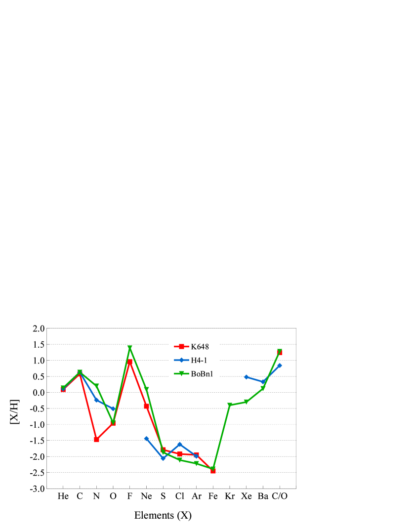
Figure 14.— The relative elemental abundances of K648, H4-1 and BoBn1 compared with those of the Sun. The solar Kr, Xe, and Ba abundances are from Lodders (2003). See Table 19 for the elemental abundances of each PN.

Table 19 Comparison of the abundances for K648, H4-1, and BoBn1.

Elements	K648	H4-1	BoBn1	Average
He	11.02$\pm$0.03	11.03$\pm$0.15	11.07$\pm$0.01	11.04$\pm$0.06
C	8.97$\pm$0.17	9.02$\pm$0.18	9.02$\pm$0.08	9.00$\pm$0.14
N	6.36$\pm$0.10	7.59$\pm$0.04	8.03$\pm$0.10	7.69$\pm$0.09
O	7.73$\pm$0.03	8.18$\pm$0.02	7.74$\pm$0.03	7.94$\pm$0.02
F	5.42$\pm$0.03	$\cdots$	5.85$\pm$0.09	5.68$\pm$0.09
Ne	7.44$\pm$0.03	6.43$\pm$0.10	7.96$\pm$0.02	7.60$\pm$0.03
S	5.40$\pm$0.07	5.13$\pm$0.03	5.32$\pm$0.16	5.30$\pm$0.09
Cl	3.58$\pm$0.15	3.88$\pm$0.13	3.39$\pm$0.07	3.66$\pm$0.12
Ar	4.60$\pm$0.13	4.56$\pm$0.12	4.33$\pm$0.04	4.51$\pm$0.10
Fe	5.02$\pm$0.12	$\cdots$	5.08$\pm$0.13	5.05$\pm$0.13
Kr	$\cdots$	$\cdots$	2.88	2.88
Xe	$\cdots$	$>$2.70	$<$2.97	2.86
Ba	$\cdots$	$\cdots$ $<$2.51	1.97	2.32
C/O	17.47$\pm$7.07	6.93$\pm$2.96	19.06$\pm$3.75	14.49$\pm$4.59

Note. — The abundances of all elements except He were determined from the CEL lines; that of He was determined from RL lines. The elemental abundances are in the form of $\log_{10}$(X/H)+12, where H is 12. The C/O number density ratio is linear value. The values of H4-1 and BoBn1 were taken from Otsuka & Tajitsu (2013) and Otsuka et al. (2010).

Otsuka et al. (2010) reported a similar comparative study of their data for BoBn1 with earlier analyses of K648. Based on incomplete observations, e.g., no detection of [F ii] lines in K648, Otsuka et al. (2010) argued that BoBn1 might have undergone binary evolution with a 0.75 $M_{\odot}$+1.5 $M_{\odot}$ system, whereas K648 might be an object that went through either a binary evolution with 0.75 $M_{\odot}$+1.5 $M_{\odot}$ or a single 1.8 $M_{\odot}$ stellar evolution, ignoring the upper limit of mass for stars in M15. Here, we refined the earlier guessing based on the abundances of 10 elements. In contrast to BoBn1, no evidence of Ba and Xe was observed in K648; however, there are similarities between BoBn1 and K648 which are not shared with H4-1. Here, we discuss similarities between K648, BoBn1 and H4-1.

Figure 14 shows the elemental abundance patterns of K648, as well as those of H4-1 and BoBn1. The abundances of all elements except He were determined based on CEL lines; the abundance of He was determined from the RL lines. Data for H4-1 and BoBn1 are from Otsuka & Tajitsu (2013) and Otsuka et al. (2010), respectively. Discrepancies in the C and O abundances in H4-1 and BoBn1 are discussed in these reports. A comparison of the RL C and O abundances among K648, H4-1 and BoBn1 is beyond the scope of this paper. The elemental abundances for each PN and the average abundance of each element are listed in Table 19.

The He and C abundances were the same for the three systems to within error. The $\alpha$-elements Ar and S, and Cl were not synthesized in significant quantities in the PN progenitors. For example, with the 1.25 $M_{\odot}$ +2.0(–3) PMZ model of Lugaro et al. (2012), an increase of only $\sim$0.02-0.03 dex was found compared with the initial abundances. Therefore, we can regard these three elements as mostly SN products. Some fractions of O and Ne are synthesized in the He-rich intershell during the TP-AGB phase. Indeed, the above 1.25 $M_{\odot}$ model Lugaro et al. (2012) predicted that such stars can increase +0.94 and +1.88 dex from the initial O and Ne abundances, respectively.

We determined gas-phase abundance of [Fe/H]=–2.45$\pm$0.12 using the ICF(Fe) in K648, which is comparable to the typical [Fe/H] abundance in a M15 star (Sobeck et al. 2011, [Fe/H]$\sim$–2.3). There are a number of other possible forms of Fe in the solid phase in laboratory experiments. According to the Jena Database of Optical Constants, for example, FeO, FeS, magnesium-iron oxides, magnesium-iron silicates, and olivine. Delgado-Inglada & Rodríguez (2014) employed a more sophisticated ionization correction factor scheme than that used here. They reported that the highest depletion factors are found in C-rich objects, exhibiting SiC around 11 $\mu$m or a broad 30 $\mu$m feature in the infrared spectra. Note that the carriers of these features are under debates. The central positions of the SiC features in the sample of Delgado-Inglada & Rodríguez (2014) were not reported, however, and K648, H4-1, and BoBn1 were not included in their sample. According to Delgado-Inglada & Rodríguez (2014), the Fe abundance ratio depletion detected in most PNe might be due to situation that less than 10 % of the Fe is in the gas phase with more than 90 % in the solid phase. Instead of using the semi-empirical ICF scheme, we have an alternative method of estimating the [Fe/H] abundance, i.e., using the Cloudy P-I model. The [Fe/H] abundance predicted using our P-I model was [Fe/H]=–1.99$\pm$0.2, which is close to that determined using the ICF method. The agreement was significantly better than that reported by Delgado-Inglada & Rodríguez (2014). The resulting ICF [Fe/H] value for K648 is likely to represent the abundance of Fe, because this value was consistent with that for typical M15 metallicity, and we did not find features corresponding to amorphous silicate, crystalline silicates, or SiC (see section 3.3.3).

There have been no reports of the detection of these features in H4-1, BoBn1, or K648. The presence of MgS and FeS is known to result in broad features around 30 $\mu$m (although the carrier of this feature remains the subject of some debate). We did not detect any other refractory element lines, such as Si and Mg, to estimate their ionized abundances in these PNe. The 1.25 $M_{\odot}$+PMZ 2(–3) $M_{\odot}$ model of Lugaro et al. (2012) predicted that the [Si/H] and [Mg/H] abundances are –2.15 and –1.67, respectively. If some of the Si and Mg-atoms might exist as dust grains, the gas-phase abundances of these two elements would become smaller, so it would be difficult to detect ionized emission-lines of these elements. The large fraction of Fe and S cannot be due to dust grains such as MgS and FeS. Therefore, the S and Fe abundances represent S and Fe in these halo PNe, and these elements are expected to exist mostly in the gas phase. However, we cannot completely exclude the possibility that some fraction of Fe resides in other solid forms.

The abundances of S, Ar, Cl, and Fe for K648 are approximately the same as those for H4-1 and BoBn1. At first, it nay be expected that all three progenitors were born in the same chemical environment during the same epoch. However, there appear to be subtle differences in the birth environments as well as the evolutionary histories.

The enhanced abundances of O, Ne, and the $n$-capture elements provide clues regarding the chemical environment where the progenitors originated and the nucleosynthesis in the inner core of the progenitors. Intrinsically larger [O/Fe] appears in metal-poor stars, which is known to be the result of the time delay effects. However, note that the observed O abundance in our sample is the sum of SN and AGB nucleosynthesized values. The O abundances in K648 and BoBn1 are approximately equal. For H4-1, however, after a detail discussion, Otsuka & Tajitsu (2013) argued that 0.2-0.3 dex of the observed $\alpha$-elements are SN products. The C/O ratio of K648 (the C-richness indicator) is very similar to that of BoBn1. The similarities of these two elements in both PNe may be explained as binary evolution and chemical enrichment during the AGB phase. Due to the O-richness, the C/O ratio of H4-1 is lower than that for the other two PNe.

The Ne abundances vary significantly amongst these halo PNe. The very small Ne abundance for H4-1 indicates that the progenitor of this PN has no PMZ. A PMZ may have been formed in the He-rich intershells of K648 and BoBn1. For BoBn1, the Ne enhancement would be due to ¹⁴N in the large PMZ and in H-burning ashes, and the ²²Ne enhancement via double $\alpha$-capturing by ¹⁴N. The enhancements of Ne and N in BoBn1 are similar ([N/H] = +0.20$\pm$0.11 and [Ne/H] = +0.09$\pm$0.10), although AGB models do not yet reproduce the N and F overabundances in BoBn1. Nonetheless, the models successfully explain both the N and F abundances in K648. K648 therefore is expected to have been born in an similar chemical environment as BoBn1, but the progenitors experienced different nucleosynthesis.

Otsuka & Tajitsu (2013) argued that the abundance of Xe in H4-1 appears heavily polluted due to the $r$-process in Type II SNe, whereas the Xe abundance in BoBn1 is close to the theoretically predicted amount via $s$-processes in AGB nucleosynthesis; therefore, Otsuka et al. (2010) concluded that the Xe in BoBn1 is a product of $s$-processes. Therefore, the chemical environments where H4-1 and BoBn1 were formed were very different.

5. Summary

We have described observations of the PN K648 in M15 and investigated chemical abundances in the nebula, the CSPN, and dust-based regions, using multiwavelength data. We determined 10 elemental abundances for the nebula, including those for F, Cl, and Fe, which are reported here for K648 for the first time. The F enhancement in K648 is comparable to that for the C-rich halo PN BoBn1. We determined the C and O abundances from both CELs and RLs. The RL C abundance was consistent with the CEL value, whereas the RL O abundance was approximately three times larger than that of the O CELs. We attempted to obtain Ne abundance more accurately by adding the Ne⁺ abundance determined using the Spitzer data. We determined the abundances of He, C, N, O, Ne, P and Fe, as well as the physical parameters of the CSPN, by employing a spectral synthesis fitting method. We found that the C/O and Ne/O ratios of the CSPN are roughly consistent with those of the nebula determined from the CELs and RLs within the error. The similar C/O ratios might indicate that the nebular abundances are reflective of the most recent stellar wind ejection from the central stellar surface. Spitzer/IRS shows the Class B 6-9 $\mu$m and 11.3 $\mu$m PAHs, as well as the broad 11 $\mu$m feature in K648.

We constructed a Cloudy radiative transfer P-I model to investigate physical conditions of the gas and dust in a self-consistent manner, and estimated the respective masses. The observed chemical abundances and core-mass of K648 are in agreement with AGB nucleosynthesis models for initial 1.25 $M_{\odot}$+PMZ = 2$\times$10^-3 $M_{\odot}$ stars, as well as initial 1.5 $M_{\odot}$ stars without PMZ. Our simulation result confirms a possibility that K648 had evolved from a star with a mass in the range of 1.25-1.5 $M_{\odot}$. Perhaps the progenitor of K648 experienced coalescence (or a large mass-transfer from its companion) during the early stages of evolution, and became a $\sim$1.25-1.5 $M_{\odot}$ blue straggler (BS). If K648 is a PN that evolved from such a BS in M15, it would be a very rare or the first such case identified among BS stars in M15, given that the expected number of PNe that evolved from BSs to date is only 0.135-0.675.

We performed the analysis of all observational data available, across a wide range of instruments and telescopes from the UV to the infrared for K648 with the help of P-I model construction. Based on our analysis, we proposed that K648 could be evolved from a BS. The BS evolution scenario into a C-rich PN is still at the speculative stage. A detailed hydrodynamic simulation may help to visualize the population-based chemical evolution, or assist in understanding the evolution of the progenitor. The most appealing scenario for K648 is that the progenitor was a close binary system that experienced coalescence or tidal disruption while both stars were in the MS stages and one emerged as a new star with a mass of $\leq$1.6 $M_{\odot}$, which then started a new life as the progenitor of K648. This progenitor passed through the AGB phase stage, and finally became the presently observable C-rich PN K648.

Appendix A Appendix

A.1. HDS optical spectra

Table ADetected nebular lines and identification of the HDS spectra.

$\lambda_{\rm obs}$	Ion	$\lambda_{\rm lab}$	Comp.	$f$($\lambda$)	$I$($\lambda$)	$\delta$$I$($\lambda$)	$\lambda_{\rm obs}$	Ion	$\lambda_{\rm lab}$	Comp.	$f$($\lambda$)	$I$($\lambda$)	$\delta$$I$($\lambda$)
(Å)		(Å)					(Å)		(Å)
3655.29	H37	3656.66	1	0.336	0.043	0.010	4879.13	[Fe iii]	4881.11	1	–0.005	0.051	0.004
3655.88	H36	3657.27	1	0.336	0.074	0.013	4920.01	He i	4921.93	1	–0.016	1.290	0.005
3656.55	H35	3657.92	1	0.336	0.031	0.011	4929.28	[O iii]	4931.23	1	–0.019	0.038	0.005
3657.20	H34	3658.64	1	0.336	0.114	0.015	4956.85	[O iii]	4958.91	1	–0.026	26.803	4.845
3657.98	H33	3659.42	1	0.336	0.130	0.016	4957.06	[O iii]	4958.91	2	–0.026	48.170	5.549
3658.89	H32	3660.28	1	0.335	0.202	0.018				Tot.		74.974	7.367
3659.77	H31	3661.22	1	0.335	0.190	0.012	4970.02	[O iii]	4958.91	1	–0.029	0.011	0.003
3660.84	H30	3662.26	1	0.335	0.275	0.023	4975.43	O v?	4977.25	1	–0.030	0.055	0.003
3661.97	H29	3663.40	1	0.335	0.379	0.021	5004.78	[O iii]	5006.84	1	–0.038	74.252	5.601
3663.26	H28	3664.68	1	0.334	0.337	0.025	5004.96	[O iii]	5006.84	2	–0.038	153.010	7.626
3664.66	H27	3666.10	1	0.334	0.437	0.023				Tot.		227.263	9.462
3666.27	H26	3667.68	1	0.334	0.366	0.023	5029.97	C ii	5032.13	1	–0.044	0.071	0.005
3668.03	H25	3669.46	1	0.334	0.421	0.026	5033.87	C ii	5035.94	1	–0.045	0.035	0.004
3670.04	H24	3671.48	1	0.333	0.486	0.027	5045.78	He i	5047.74	1	–0.048	0.187	0.003
3672.31	H23	3673.76	1	0.333	0.535	0.019	5059.64	N iv?	5061.62	1	–0.051	0.039	0.003
3674.93	H22	3676.36	1	0.332	0.619	0.019	5119.81	C ii	5121.83	1	–0.065	0.033	0.004
3677.91	H21	3679.35	1	0.332	0.697	0.020	5515.51	[Cl iii]	5517.72	1	–0.145	0.021	0.003
3681.36	H20	3682.81	1	0.331	0.713	0.020	5535.63	[Cl iii]	5537.89	1	–0.149	0.028	0.003
3685.38	H19	3686.83	1	0.330	0.840	0.029	5752.41	[N ii]	5754.64	1	–0.185	0.043	0.002
3690.11	H18	3691.55	1	0.329	1.001	0.028	5873.37	He i	5875.62	1	–0.203	14.834	0.138
3695.70	H17	3697.15	1	0.328	1.216	0.026	5907.09	Si i	5909.37	1	–0.208	0.013	0.002
3702.42	H16	3703.85	1	0.327	1.407	0.031	5977.50	S ii	5979.76	1	–0.218	0.016	0.001
3703.59	He i	3705.14	1	0.327	0.722	0.026	6148.93	C ii	6151.27	1	–0.242	0.045	0.003
3710.52	H15	3711.97	1	0.325	1.534	0.027	6234.73	C i	6237.23	1	–0.254	0.022	0.001
3720.48	H14	3721.94	1	0.323	1.937	0.033	6236.13	Fe ii	6238.39	1	–0.254	0.014	0.001
3724.63	[O ii]	3726.03	1	0.322	7.729	0.156	6236.39	Ne ii	6238.92	1	–0.254	0.023	0.001
3724.61	[O ii]	3726.03	2	0.322	9.654	0.255	6257.02	C ii	6259.56	1	–0.257	0.009	0.003
			Tot.		17.383	0.299	6257.37	C ii	6259.56	1	–0.257	0.013	0.001
3727.40	[O ii]	3728.81	1	0.322	3.047	0.166	6297.90	[O i]	6300.30	1	–0.263	0.225	0.008
3727.36	[O ii]	3728.81	2	0.322	6.340	0.309	6298.44	[O i]	6300.30	2	–0.263	0.041	0.007
			Tot.		9.387	0.350				Tot.		0.266	0.011
3732.90	H13	3734.37	1	0.321	2.428	0.040	6309.60	[S iii]	6313.10	1	–0.264	0.119	0.005
3748.69	H12	3750.15	1	0.317	2.968	0.043	6361.31	[O i]	6363.78	1	–0.271	0.068	0.003
3769.16	H11	3770.63	1	0.313	3.934	0.052	6459.20	C ii	6462.04	1	–0.284	0.076	0.007
3796.41	H10	3797.90	1	0.307	5.291	0.067	6459.61	C ii	6462.04	2	–0.284	0.022	0.005
3818.13	He i	3819.60	1	0.302	0.911	0.015				Tot.		0.098	0.009
3833.89	H9	3835.38	1	0.299	7.105	0.089	6522.88	Ne ii	6525.59	1	–0.293	0.014	0.001
3867.22	[Ne iii]	3869.06	1	0.291	9.939	0.124	6545.56	[N ii]	6548.04	1	–0.296	0.901	0.012
3887.32	H8	3889.05	1	0.286	22.451	0.456	6559.94	H3	6562.82	1	–0.298	119.758	3.906
3917.39	C ii	3918.97	1	0.279	0.078	0.011	6560.45	H3	6562.82	2	–0.298	162.641	4.167
3919.12	C ii	3920.68	1	0.279	0.167	0.012				Tot.		282.399	5.712
3925.02	He i	3926.54	1	0.277	0.137	0.013	6575.48	C ii	6578.05	1	–0.300	0.692	0.011
3963.20	He i	3964.73	1	0.267	0.780	0.015	6580.77	[N ii]	6583.46	1	–0.300	1.488	0.032
3965.89	[Ne iii]	3967.79	1	0.267	3.147	0.043	6580.93	[N ii]	6583.46	2	–0.300	1.692	0.025
3968.60	H7	3970.07	1	0.266	10.703	0.167				Tot.		3.180	0.041
3971.08	C ii	3972.45	1	0.265	0.144	0.015	6604.63	Ne ii	6607.40	1	–0.303	0.023	0.003
3997.69	C iii	3999.64	1	0.258	0.035	0.008	6628.07	O iv	6630.70	1	–0.307	0.010	0.001
4007.72	He i	4009.26	1	0.256	0.191	0.014	6675.56	He i	6678.15	1	–0.313	4.114	0.055
4024.64	He i	4026.18	1	0.251	1.958	0.024	6712.28	N ii	6714.99	1	–0.318	0.032	0.003
4074.57	[S ii]	4076.35	1	0.237	0.111	0.031	6713.90	[S ii]	6716.44	1	–0.318	0.087	0.002
4079.83	O iii	4081.00	1	0.235	0.034	0.008	6724.89	C iii	6727.48	1	–0.319	0.037	0.003
4100.13	H6	4101.73	1	0.230	26.339	0.248	6728.30	[S ii]	6730.81	1	–0.320	0.133	0.003
4119.23	He i	4120.81	1	0.224	0.202	0.013	6731.54	He i	6734.08	1	–0.320	0.022	0.003
4142.10	He i	4143.76	1	0.217	0.156	0.006	6739.57	C iii	6742.15	1	–0.321	0.041	0.004
4265.50	C ii	4267.18	1	0.180	0.660	0.016	6741.76	C iii	6744.39	1	–0.322	0.061	0.003
4265.51	C ii	4267.18	1	0.180	0.726	0.013	6777.39	C ii	6780.60	1	–0.326	0.059	0.003
4338.77	H5	4340.46	1	0.157	46.674	0.307	6798.18	C ii	6800.68	1	–0.329	0.052	0.006
4361.49	[O iii]	4363.21	1	0.149	2.782	0.026	6931.26	He i	6933.89	1	–0.347	0.053	0.003
4386.21	He i	4387.93	1	0.142	0.517	0.010	7034.62	C iii	7037.25	1	–0.361	0.075	0.003
4435.82	He i	4437.55	1	0.126	0.088	0.013	7059.60	He i	7062.28	1	–0.364	0.026	0.003
4469.76	He i	4471.47	1	0.115	4.914	0.028	7062.49	He i	7065.18	1	–0.364	5.909	0.100
4636.98	O ii	4638.86	1	0.064	0.055	0.006	7092.65	Si i	7095.49	1	–0.368	0.015	0.005
4640.01	O ii	4641.81	1	0.063	0.033	0.003	7096.05	N iv?	7098.60	1	–0.369	0.020	0.002
4701.53	[Fe iii]	4701.53	1	0.045	0.022	0.003	7132.99	[Ar iii]	7135.70	1	–0.374	0.384	0.006
4706.34	N ii	4708.28	1	0.043	0.030	0.003	7278.53	He i	7281.39	1	–0.393	0.598	0.008
4711.34	He i	4713.14	1	0.042	0.672	0.005	7316.27	[O ii]	7319.14	1	–0.398	0.452	0.020
4787.73	[F ii]	4789.45	1	0.020	0.110	0.004	7317.32	[O ii]	7320.19	1	–0.398	1.340	0.015
4859.43	H4	4861.33	1	0.000	100.000	0.188	7326.89	[O ii]	7329.76	1	–0.400	0.745	0.015
4867.28	[F ii]	4868.99	1	–0.002	0.030	0.003	7327.95	[O ii]	7330.82	1	–0.400	0.705	0.015

References

- Abia et al. (2002) Abia, C., Domínguez, I., Gallino, R., et al. 2002, ApJ, 579, 817
- Acker et al. (2002) Acker, A., Gesicki, K., Grosdidier, Y., & Durand, S. 2002, A&A, 384, 620
- Adams et al. (1984) Adams, S., Seaton, M. J., Howarth, I. D., Auriere, M., & Walsh, J. R. 1984, MNRAS, 207, 471
- Aldrovandi (1980) Aldrovandi, S. M. V. 1980, Ap&SS, 71, 393
- Alves et al. (2000) Alves, D. R., Bond, H. E., & Livio, M. 2000, AJ, 120, 2044
- Asplund et al. (2009) Asplund, M., Grevesse, N., Sauval, A. J., & Scott, P. 2009, ARA&A, 47, 481
- Barker (1983) Barker, T. 1983, ApJ, 270, 641
- Beers & Christlieb (2005) Beers, T. C., & Christlieb, N. 2005, ARA&A, 43, 531
- Benjamin et al. (1999) Benjamin, R. A., Skillman, E. D., & Smits, D. P. 1999, ApJ, 514, 307
- Bernard-Salas et al. (2009) Bernard-Salas, J., Peeters, E., Sloan, G. C., et al. 2009, ApJ, 699, 1541
- Bernard-Salas et al. (2003) Bernard-Salas, J., Pottasch, S. R., Wesselius, P. R., & Feibelman, W. A. 2003, A&A, 406, 165
- Bianchi et al. (2001) Bianchi, L., Bohlin, R., Catanzaro, G., Ford, H., & Manchado, A. 2001, AJ, 122, 1538
- Bianchi et al. (1995) Bianchi, L., Ford, H., Bohlin, R., Paresce, F., & de Marchi, G. 1995, A&A, 301, 537
- Bisterzo et al. (2012) Bisterzo, S., Gallino, R., Straniero, O., Cristallo, S., & Käppeler, F. 2012, MNRAS, 422, 849
- Bohren & Huffman (1983) Bohren, C. F., & Huffman, D. R. 1983, Absorption and scattering of light by small particles (New York: Wiley)
- Bouret et al. (2003) Bouret, J.-C., Lanz, T., Hillier, D. J., et al. 2003, ApJ, 595, 1182
- Boyer et al. (2006) Boyer, M. L., Woodward, C. E., van Loon, J. T., et al. 2006, AJ, 132, 1415
- Cardelli et al. (1989) Cardelli, J. A., Clayton, G. C., & Mathis, J. S. 1989, ApJ, 345, 245
- Costa et al. (1996) Costa, R. D. D., Chiappini, C., Maciel, W. J., & de Freitas Pacheco, J. A. 1996, A&AS, 116, 249
- Delgado-Inglada et al. (2014) Delgado-Inglada, G., Morisset, C., & Stasińska, G. 2014, MNRAS, 440, 536
- Delgado-Inglada & Rodríguez (2014) Delgado-Inglada, G., & Rodríguez, M. 2014, ApJ, 784, 173
- Díaz-Sánchez et al. (2012) Díaz-Sánchez, A., Pérez-Garrido, A., Villó, I., et al. 2012, MNRAS, 423, 2260
- Dieball et al. (2007) Dieball, A., Knigge, C., Zurek, D. R., et al. 2007, ApJ, 670, 379
- Draine & Li (2007) Draine, B. T., & Li, A. 2007, ApJ, 657, 810
- Fazio et al. (2004) Fazio, G. G., Hora, J. L., Allen, L. E., et al. 2004, ApJS, 154, 10
- Feldmeier (2003) Feldmeier, J. J. 2003, in IAU Symposium, Vol. 209, Planetary Nebulae: Their Evolution and Role in the Universe, ed. S. Kwok, M. Dopita, & R. Sutherland, 597
- Feltzing & Chiba (2013) Feltzing, S., & Chiba, M. 2013, New A Rev., 57, 80
- Ferland et al. (1998) Ferland, G. J., Korista, K. T., Verner, D. A., et al. 1998, PASP, 110, 761
- Ferraro et al. (2009) Ferraro, F. R., Beccari, G., Dalessandro, E., et al. 2009, Nature, 462, 1028
- Fluks et al. (1994) Fluks, M. A., Plez, B., The, P. S., et al. 1994, A&AS, 105, 311
- García-Segura et al. (1999) García-Segura, G., Langer, N., Różyczka, M., & Franco, J. 1999, ApJ, 517, 767
- Gesicki et al. (2003) Gesicki, K., Acker, A., & Zijlstra, A. A. 2003, A&A, 400, 957
- Hawley & Miller (1978) Hawley, S. A., & Miller, J. S. 1978, ApJ, 220, 609
- Henry et al. (1996) Henry, R. B. C., Kwitter, K. B., & Howard, J. W. 1996, ApJ, 458, 215
- Higdon et al. (2004) Higdon, S. J. U., Devost, D., Higdon, J. L., et al. 2004, PASP, 116, 975
- Houck et al. (2004) Houck, J. R., Roellig, T. L., van Cleve, J., et al. 2004, ApJS, 154, 18
- Howard et al. (1997) Howard, J. W., Henry, R. B. C., & McCartney, S. 1997, MNRAS, 284, 465
- Jacoby et al. (2013) Jacoby, G. H., Ciardullo, R., De Marco, O., et al. 2013, ApJ, 769, 10
- Jacoby et al. (1997) Jacoby, G. H., Morse, J. A., Fullton, L. K., Kwitter, K. B., & Henry, R. B. C. 1997, AJ, 114, 2611
- Kalirai et al. (2008) Kalirai, J. S., Hansen, B. M. S., Kelson, D. D., et al. 2008, ApJ, 676, 594
- Karakas (2010) Karakas, A. I. 2010, MNRAS, 403, 1413
- Kingsburgh & Barlow (1992) Kingsburgh, R. L., & Barlow, M. J. 1992, MNRAS, 257, 317
- Kobayashi et al. (2011) Kobayashi, C., Karakas, A. I., & Umeda, H. 2011, MNRAS, 414, 3231
- Kwitter et al. (2003) Kwitter, K. B., Henry, R. B. C., & Milingo, J. B. 2003, PASP, 115, 80
- Kwok et al. (2001) Kwok, S., Volk, K., & Bernath, P. 2001, ApJ, 554, L87
- Lanz & Hubeny (2003) Lanz, T., & Hubeny, I. 2003, ApJS, 146, 417
- Lattanzio (1987) Lattanzio, J. C. 1987, ApJ, 313, L15
- Leisenring et al. (2008) Leisenring, J. M., Kemper, F., & Sloan, G. C. 2008, ApJ, 681, 1557
- Li & Draine (2012) Li, A., & Draine, B. T. 2012, ApJ, 760, L35
- Liu (1998) Liu, X.-W. 1998, MNRAS, 295, 699
- Liu et al. (2001) Liu, X.-W., Luo, S.-G., Barlow, M. J., Danziger, I. J., & Storey, P. J. 2001, MNRAS, 327, 141
- Liu et al. (2000) Liu, X.-W., Storey, P. J., Barlow, M. J., et al. 2000, MNRAS, 312, 585
- Lodders (2003) Lodders, K. 2003, ApJ, 591, 1220
- Lugaro et al. (2012) Lugaro, M., Karakas, A. I., Stancliffe, R. J., & Rijs, C. 2012, ApJ, 747, 2
- Luridiana et al. (2003) Luridiana, V., Pérez, E., & Cerviño, M. 2003, AJ, 125, 3196
- Masseron et al. (2010) Masseron, T., Johnson, J. A., Plez, B., et al. 2010, A&A, 509, A93
- Mathis et al. (1977) Mathis, J. S., Rumpl, W., & Nordsieck, K. H. 1977, ApJ, 217, 425
- McCarthy et al. (1990) McCarthy, J. K., Mould, J. R., Mendez, R. H., et al. 1990, ApJ, 351, 230
- McNamara et al. (2004) McNamara, B. J., Harrison, T. E., & Baumgardt, H. 2004, ApJ, 602, 264
- McWilliam (1997) McWilliam, A. 1997, ARA&A, 35, 503
- Min et al. (2003) Min, M., Hovenier, J. W., & de Koter, A. 2003, A&A, 404, 35
- Moe & De Marco (2006) Moe, M., & De Marco, O. 2006, ApJ, 650, 916
- Molster et al. (2001) Molster, F. J., Lim, T. L., Sylvester, R. J., et al. 2001, A&A, 372, 165
- Morisset & Georgiev (2009) Morisset, C., & Georgiev, L. 2009, A&A, 507, 1517
- Nishimura et al. (2009) Nishimura, T., Aikawa, M., Suda, T., & Fujimoto, M. Y. 2009, PASJ, 61, 909
- Noguchi et al. (2002) Noguchi, K., Aoki, W., Kawanomoto, S., et al. 2002, PASJ, 54, 855
- Otsuka et al. (2009) Otsuka, M., Hyung, S., Lee, S.-J., Izumiura, H., & Tajitsu, A. 2009, ApJ, 705, 509
- Otsuka et al. (2008) Otsuka, M., Izumiura, H., Tajitsu, A., & Hyung, S. 2008, ApJ, 682, L105
- Otsuka et al. (2014) Otsuka, M., Kemper, F., Cami, J., Peeters, E., & Bernard-Salas, J. 2014, MNRAS, 437, 2577
- Otsuka et al. (2013) Otsuka, M., Kemper, F., Hyung, S., et al. 2013, ApJ, 764, 77
- Otsuka & Tajitsu (2013) Otsuka, M., & Tajitsu, A. 2013, ApJ, 778, 146
- Otsuka et al. (2010) Otsuka, M., Tajitsu, A., Hyung, S., & Izumiura, H. 2010, ApJ, 723, 658
- Peeters et al. (2002) Peeters, E., Hony, S., Van Kerckhoven, C., et al. 2002, A&A, 390, 1089
- Pegourie (1988) Pegourie, B. 1988, A&A, 194, 335
- Peimbert et al. (2005) Peimbert, A., Peimbert, M., & Ruiz, M. T. 2005, ApJ, 634, 1056
- Peimbert (1967) Peimbert, M. 1967, ApJ, 150, 825
- Peimbert (1978) Peimbert, M. 1978, in IAU Symposium, Vol. 76, Planetary Nebulae, ed. Y. Terzian, 215–223
- Péquignot & Tsamis (2005) Péquignot, D., & Tsamis, Y. G. 2005, A&A, 430, 187
- Pereira & Miranda (2007) Pereira, C.-B., & Miranda, L.-F. 2007, A&A, 467, 1249
- Poglitsch et al. (2010) Poglitsch, A., Waelkens, C., Geis, N., et al. 2010, A&A, 518, L2
- Pottasch et al. (2011) Pottasch, S. R., Surendiranath, R., & Bernard-Salas, J. 2011, A&A, 531, A23
- Pottasch et al. (2009) Pottasch, S. R., Surendiranath, R., Bernard-Salas, J., & Roellig, T. L. 2009, A&A, 502, 189
- Prada Moroni & Straniero (2007) Prada Moroni, P. G., & Straniero, O. 2007, A&A, 466, 1043
- Quireza et al. (2007) Quireza, C., Rocha-Pinto, H. J., & Maciel, W. J. 2007, A&A, 475, 217
- Rauch et al. (2002) Rauch, T., Heber, U., & Werner, K. 2002, A&A, 381, 1007
- Reddy et al. (1999) Reddy, B. E., Bakker, E. J., & Hrivnak, B. J. 1999, ApJ, 524, 831
- Reid (1996) Reid, I. N. 1996, AJ, 111, 2000
- Rieke et al. (2004) Rieke, G. H., Young, E. T., Engelbracht, C. W., et al. 2004, ApJS, 154, 25
- Rouleau & Martin (1991) Rouleau, F., & Martin, P. G. 1991, ApJ, 377, 526
- Shingles & Karakas (2013) Shingles, L. J., & Karakas, A. I. 2013, MNRAS, 431, 2861
- Shipman (1979) Shipman, H. L. 1979, ApJ, 228, 240
- Sills et al. (1997) Sills, A., Lombardi, Jr., J. C., Bailyn, C. D., et al. 1997, ApJ, 487, 290
- Sloan et al. (2003) Sloan, G. C., Kraemer, K. E., Price, S. D., & Shipman, R. F. 2003, ApJS, 147, 379
- Sobeck et al. (2011) Sobeck, J. S., Kraft, R. P., Sneden, C., et al. 2011, AJ, 141, 175
- Stanghellini et al. (2012) Stanghellini, L., García-Hernández, D. A., García-Lario, P., et al. 2012, ApJ, 753, 172
- Storey & Hummer (1995) Storey, P. J., & Hummer, D. G. 1995, MNRAS, 272, 41
- Tajitsu & Otsuka (2004) Tajitsu, A., & Otsuka, M. 2004, in Astronomical Society of the Pacific Conference Series, Vol. 313, Asymmetrical Planetary Nebulae III: Winds, Structure and the Thunderbird, ed. M. Meixner, J. H. Kastner, B. Balick, & N. Soker, 202
- Tajitsu & Otsuka (2006) Tajitsu, A., & Otsuka, M. 2006, in IAU Symposium, Vol. 234, Planetary Nebulae in our Galaxy and Beyond, ed. M. J. Barlow & R. H. Méndez, 523–524
- Tajitsu & Otsuka (2014) Tajitsu, A., & Otsuka, M. 2014, ApJ, submitted