Perfect wave-packet splitting and reconstruction in a one-dimensional lattice

Abstract

Particle delocalization is a common feature of quantum random walks in arbitrary lattices. However, in the typical scenario a particle spreads over multiple sites and its evolution is not directly useful for controlled quantum interferometry, as may be required for technological applications. In this paper we devise a strategy to perfectly split the wave-packet of an incoming particle into two components, each propagating in opposite directions, which reconstruct the shape of the initial wavefunction after a particular time $t^{*}$. Therefore, a particle in a delta-like initial state becomes exactly delocalized between two distant sites after $t^{*}$. We find the mathematical conditions to achieve the perfect splitting which are satisfied by viable example Hamiltonians with static site-dependent interaction strengths. Our results pave the way for the generation of peculiar many-body interference patterns in a many-site atomic chain (like the Hanbury Brown and Twiss and quantum Talbot effects) as well as for the distribution of entanglement between remote sites. Thus, as for the case of perfect state transfer, the perfect wave-packet splitting can be a new tool for varied applications.

I Introduction

The quest for a quantum computer is boosting the development and engineering of new sophisticated quantum devices that allow us to observe the space-time evolution of its constituents. Indeed, in recent years several experimental groups successfully measured the quantum dynamical evolution of particles and/or quasi-particle hopping in a lattice Preiss et al. (2014); Fukuhara et al. (2013a, b); Sansoni et al. (2012); Ramanathan et al. (2011); Schreiber et al. (2015); Richerme et al. (2014); Schachenmayer et al. (2013); Trompeter et al. (2006). Due to the inherent nature of quantum mechanics, the evolution of an isolated quantum system is represented by a wavefunction $\psi(x,t)$ which describes the probability amplitude of finding a particle in position $x$ at time $t$. Quantum interference can give rise to particular structures and patterns in the space-time evolution $|\psi(x,t)|^{2}$ which are known as “quantum carpets” Kaplan et al. (2000), quantum revivals Robinett (2004), or quantum Talbot effect Berry et al. (2001), quantum walks Kempe (2003); Childs (2009); Childs et al. (2003), and quantum self-imaging Longhi (2010).

An interesting case is when the wavefunction undergoes a revival, namely when after a particular time the shape of the initial wave packet is almost perfectly reconstructed. Aside from its fundamental implication, revivals occurring into a different position, far from the initial one, are particularly important for connecting and linking distant quantum registers Cirac et al. (1997); Ritter et al. (2012). On the other hand, a lattice of static localized particles represents an alternative paradigm for quantum communication where information carriers are not physically moving particles but rather collective excitations whose space extent is reconstructed at a different position after a certain time. In this respect, spin chains represent one of the most viable solution and there are various protocols to exploit their dynamics for transferring states and entanglement between remote sites Bose (2007); Nikolopoulos and Jex (2013). The coherent excitation transfer, or in general the wavefunction reconstruction at a certain time, corresponds to the phase alignment of the eigenstates entering into the wave packet and, as such, can happen only when the energy eigenvalues satisfy certain conditions Aronstein and Stroud (1997); Kay (2010). Some models admitting a perfect Albanese et al. (2004); Aronstein and Stroud (1997); Yung and Bose (2005) or almost perfect Godsil et al. (2012); Banchi (2013); Banchi et al. (2011); Yao et al. (2011) reconstruction have been explicitly constructed. On the other hand, if the phase alignment is only between particular subsets of the energy eigenstates, then the wavefunction is split into a superposition of copies of the initial wave-packet, each separated by a certain distance. This effect is known as fractional revival Aronstein and Stroud (1997); Chen et al. (2007); Robinett (2004), or fractional Talbot effect Berry et al. (2001).

In this paper we engineer a chain with nearest neighbor interactions to obtain a perfect wave-packet splitting and reconstruction during a ballistic evolution. In other terms, if $\psi(x,t{=}0){=}f(x)$ is the shape of the initial wave-packet, at the revival time $t^{*}$ the wavefunction is $\psi(x,t){=}\frac{f(x{-}vt^{*}){+}f(x{+}vt^{*})}{\sqrt{2}}$, where $v$ is the group velocity defined by the energy eigenvalues. While in general the revival time is connected to specific algebraic properties of the spectrum and might be very long, in our case the splitting happens on a time which is dictated by the group velocity of excitations and, as such, scales only linearly with the distance. Our method is therefore specifically targeted for applications where a smaller operational time is particularly important for neglecting the interaction with the surrounding environment. Recently, it has been shown that the wavefunction of a one-dimensional excitation can be split into a transmitted and reflected components by introducing localized impurities Compagno et al. (2014); Fogarty et al. (2013); Gertjerenken (2013), or via suitably designed time-dependent control fields Makin et al. (2012). Here we focus on a different strategy aiming at obtaining a perfect fractional revival.

The generalization of the fractional revival to a many-particle setting has many important applications. As far as identical particles (bosons/fermions) are concerned, it allows one to define a perfect effective beam splitter operation between distant sites and then to observe multi-particle Hanbury Brown and Twiss interference effects Brown and Twiss (1956), such as perfect bunching or anti-bunching. As for spin systems, that the perfect fractional revival can be used to generate dynamically long-distance entanglement, a topical application which may be tested experimentally with current technology Mitra (2015); Sahling et al. (2015). Indeed, the use of particle delocalization to generate entanglement is particularly evident in a single excitation setup, namely when there is a single spin in the state $|{\uparrow}\rangle$ while all the other spins are in the state $|{\downarrow}\rangle$. If the wave-packet of this excitation is perfectly split and reconstructed in two distant sites $n$ and $m$, then the final state of the spins pair $(n,m)$ is $(|{\uparrow\downarrow}\rangle_{nm}+|{\downarrow\uparrow}\rangle_{nm})/\sqrt{2}$, namely a maximally entangled Bell state. We show that this reasoning can also be used in a multiple excitation scenario to dynamically generate a maximal set of Bell pairs in a spin chain setup, and to provide a more general version of previous proposals Alkurtass et al. (2014); Di Franco et al. (2008).

This paper is organized as follows. In section II, we define the mathematical conditions which allows a particular fractional revival, namely the perfect splitting and reconstruction of an incoming wave packet, and we propose a numerical algorithm to find suitable Hamiltonians which fulfill these conditions. Interesting applications are then analyzed in section III in a many-particle setting. In particular, we discuss bunching/anti-bunching effects in atoms trapped in an optical lattice and the dynamical generation of entanglement in spin chains interacting with nearest-neighbor XY couplings. Conclusions are drawn in section IV.

II Perfect splitting with engineered couplings

We study a one-dimensional quantum walk in a lattice with nearest-neighbor engineered interactions described by the Hamiltonian

$$H_{p}=-\left(\sum_{n=1}^{L-1}J_{n}|{n}\rangle\langle{n{+}1}|+{\rm h.c.}\right)-\sum_{n=1}^{L}B_{n}|{n}\rangle\langle{n}|~{},$$ (1)

where $|{n}\rangle$ represents the state where a particle is in the $n$-th site, and $L$ is the length of the chain. To find the mathematical conditions for a perfect splitting and reconstruction, we first focus on the requirements to achieve perfect state transfer. To perfectly transfer an excitation from site 1 to site $L$ the coefficients $J_{n}$ and $B_{n}$ have to satisfy some conditions (see e.g. Ref.Kay (2010)). Firstly, the Hamiltonian has to be mirror symmetric, i.e. $J_{L-n}{=}J_{n}$ and $B_{L+1-n}{=}B_{n}$ for any $1{\leq}n{\leq}L$. The mirror symmetry imposes some relations between the eigenvectors of the Hamiltonian Yung and Bose (2005): if the eigenvalues $E_{k}$ of $H_{p}$ are ordered such that $E_{k}{<}E_{k+1}$, then

$$O_{Lk}=(-1)^{k}O_{1k}~{},$$ (2)

where $H_{p}=OEO^{T}$ is the eigenvalue decomposition of $H_{p}$. The second requirement is that the energy eigenvalues $E_{k}$ satisfy the relation

$$e^{-iE_{k}t^{*}}=(-1)^{k}e^{i\alpha}~{},$$ (3)

where $t^{*}$ is the transmission time and $\alpha$ is an arbitrary phase. Here we consider $\alpha{=}0$, namely ${\rm Tr}H{=}0$. Among the analytic solutions of (3), the simplest one is given by the coupling pattern Christandl et al. (2004); Albanese et al. (2004)

$$J_{n}^{\rm PST} =\frac{\pi J}{2L}\sqrt{n(L-n)}~{}, B_{n} =0~{},$$ (4)

which implements perfect state transfer (PST) at $t^{*}{=}L{/}J$. Other solutions can be obtained numerically using inverse eigenvalue algorithms Kay (2006, 2010); Bruderer et al. (2012). If the eigenvalues and eigenvectors of $H_{p}$ satisfy Eqs.(2) and (3), then

$$\langle{n}|e^{-iH_{p}t^{*}}|{m}\rangle =\sum_{k}O_{n,k}O_{m,k}e^{-iE_{k}t^{*}}=\sum_{k}O_{n,k}O_{m,k}(-1)^{k}$$

$$=\sum_{k}O_{n,k}O_{L+1-m,k}=\delta_{n,L+1-m}~{},$$ (5)

namely an excitation initially located in site $m$ is perfectly transferred to site $L{-}m{+}1$ after a time $t^{*}$.

In a similar fashion, a perfect wave-packet splitting and reconstruction can be obtained when the eigenvalues of $H_{p}$ satisfy

$$e^{-iE_{k}t^{*}}=\cos\theta+i(-1)^{k}\sin\theta~{},$$ (6)

for some angle $\theta$. Indeed, by repeating the calculation (5) one finds $\langle{n}|e^{-iH_{p}t^{*}}|{m}\rangle{=}\cos\theta\;\delta_{nm}{+}i\sin\theta\;\delta_{n,L+1-m}~{},$ namely

$$|{m}\rangle\xrightarrow{t^{*}}\cos\theta|{m}\rangle+i\sin\theta|{L{-}m{+}1}\rangle~{}.$$ (7)

The eigenvalue relations (6) are one of the main result of this paper. By properly choosing $\theta$ it is possible to balance the reconstruction on distant sites, as show in Eq.(7), and for $\pi{=}\pi{/}4$ one obtains the perfect delocalization between distant sites of an initially localized wave packet. The coupling pattern to satisfy Eq.(6) can be obtained using inverse eigenvalue techniques. From the conceptual point of view an inverse eigenvalue problem deals with finding the zeros of the highly non-linear function $f(\lambda){=}E(\lambda){-}\tilde{E}$, where the vector $E(\lambda)$ contains the ordered eigenvalues of the Hamiltonian $H_{p}(\lambda)$ with parameters $\lambda$, and the vector $\tilde{E}$ contains the target spectrum. Among the algorithms to find the optimal parameters Parlett (1998); Chu (1998), the most used one relies on the application of the Newton method to find the zeros of $f(\lambda)$. The Newton method starts with an initial guess $\lambda^{(0)}$ and updates it according to the rule Friedland et al. (1987)

$$\mathcal{J}(\lambda_{n})[\lambda^{(n+1)}-\lambda^{(n)}]=f(\lambda^{(n)})~{},$$ (8)

where the matrix, with elements

$$\mathcal{J}_{mk}(\lambda^{(n)})=\frac{\partial f_{m}(\lambda^{(n)})}{\partial\lambda^{(n)}_{k}}=\langle{m}|O(\lambda^{(n)})^{T}\frac{\partial H_{p}(\lambda^{(n)})}{\partial\lambda^{(n)}_{k}}O(\lambda^{(n)})|{k}\rangle~{},$$ (9)

is the Jacobian matrix and $H_{p}(\lambda){=}O(\lambda)E(\lambda)O(\lambda)^{T}$ is the eigenvalue decomposition of $H_{p}(\lambda)$. The linear system (8) has a unique solution provided that $\mathcal{J}$ is an invertible matrix. This in turn implies that the number of parameters have to match the number of eigenvalues, i.e. the dimension of the matrix.

The mirror symmetric Hamiltonian (1) has $L$ independent parameters, being $L$ the number of sites. Indeed, because of the mirror symmetry, when $L{=}2N$ (being $N$ an integer) there are $N$ independent values of $J_{n}$ and $N$ independent values of $B_{n}$. On the other hand, when $L{=}2N{+}1$, there are $N$ independent values of $J_{n}$ and $N{+}1$ independent values of $B_{n}$. We apply inverse eigenvalue techniques to find the coupling pattern which allows a perfect balanced splitting of the wave-packet. The latter is obtained by imposing the condition (6) with $\theta{=}\pi{/}4$, so the target eigenvalues are

$$\frac{L\tilde{E}}{J}=\left(\dots,-\frac{\pi}{4},\frac{\pi}{4},-\frac{\pi}{4}+2\pi,\frac{\pi}{4}+2\pi,-\frac{\pi}{4}+4\pi,\dots\right)^{T}$$ (10)

where, without loss of generality, we have imposed $t^{*}=L/J$. Because $f(\lambda)$ is in general a non-convex function, possibly with many local minima, inverse eigenvalue problems are known to converge only if the initial guess $\lambda^{(0)}$ is not too far from the ideal set of parameters $\tilde{\lambda}$ for which $E(\tilde{\lambda}){=}\tilde{E}$ Friedland et al. (1987). We guess that the optimal parameters for a perfect wave packet splitting are given by a local perturbation of the fully engineered chain which guarantees perfect state transfer, so we use the coupling pattern (4) as an initial condition.

The algorithm quickly converges to an optimal parameter set and hereinafter we called $J_{n}^{\rm split}$ and $B_{n}^{\rm split}$ the obtained optimal couplings and local fields. Surprisingly, we find that for even $L$ the algorithm always converges to a solution where $B_{n}^{\rm split}{=}0$, while for odd $L$ the local fields $B_{n}^{\rm split}$ are different from zeros especially near the center of the chain. For example, the Hamiltonians for $L{=}5{,}6$ are shown in Appendix A.

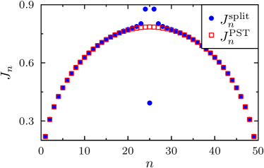
(a)  Even length chain

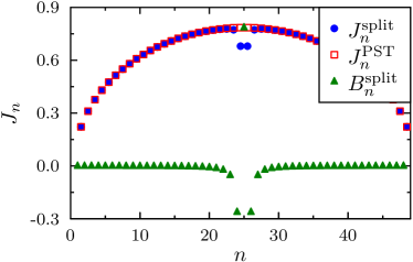
(b)  Odd length chain

Figure 1: Comparison between the perfect wave-packet splitting couplings $J_{n}^{\rm split}$ and the perfect state transfer couplings $J_{n}^{PST}$ in Eq.(4) for (a) an even chain and for an (b) odd chain. Only in the latter case the perfect splitting requires also the engineering of a field profile $B_{n}^{split}$.

The output of the algorithm is shown in Fig.1(a) for $L{=}50$, and in Fig.1(b) for $L{=}49$. As it is clear, both for $L$ even and odd the coupling patterns $J_{n}^{\rm split}$ for perfect wave-packet splitting are similar to the coupling pattern $J_{n}^{PST}$, in formula (4), for perfect state transfer: the only difference being the presence of few impurities at the center of the chain. Moreover, for odd $L$ one requires also the engineering of the local fields $B_{n}^{\rm split}$ according to some particular profile. The resulting field pattern is constant far from the center of the chain and has a particular oscillatory profile near the central sites.

III Applications

III.1 Perfect bunching/anti-bunching in a bosonic lattice

As a concrete application of the results of the last section we consider a model of hopping particle in a one-dimensional lattice, described by a Bose-Hubbard Hamiltonian with site dependent parameters

$$\mathcal{H}=-\sum\limits_{n=1}^{L}J_{n}\left(a_{n}^{\dagger}a_{n+1}+\text{h.c.}\right)+\sum\limits_{n=1}^{L}U_{n}n_{n}\left(n_{n}-1\right)-\sum_{n=1}^{L}B_{n}n_{n}.$$ (11)

Here $J_{n}{=}J_{n}^{\rm split}$ are the tunneling matrix elements, $U_{n}$ is the onsite interaction and $B_{n}{=}B_{n}^{\rm split}$ is the chemical potential, $a_{n}$ is the boson annihilation operator and $n_{j}{=}a_{j}^{\dagger}a_{j}$. The Hamiltonian (11) accurately describes cold bosonic atoms in optical lattices Jaksch et al. (1998); Greiner et al. (2002), and it also models fermions Jördens et al. (2008); Modugno et al. (2003) and hard-core bosons Rigol and Muramatsu (2004) dependently on the onsite interaction values. The tuning of the site dependent coupling constants in (11) is achieved via addressable optical lattices Wang et al. (2013), created projecting an electric field profile via holographic masks Bakr et al. (2009); Boyer et al. (2006) or via micro-mirror devices Preiss et al. (2014). Initialization and read-out of single atoms are achieved exploiting single-particle addressing techniques Preiss et al. (2014); Weitenberg et al. (2011); Endres et al. (2013); Gross and Bloch (2014); Schreiber et al. (2015) while magnetically induced Feshbach resonances allow a global control of the onsite interaction acting on the collisional coupling constants values Sanders et al. (2011). For instance the non-interacting regime $U_{n}{=}0$ has been recently achieved with this technique using $\rm Cs$ atoms loaded in a one-dimensional optical lattice Meinert et al. (2014).

Thanks to the techniques developed in this paper, the coupling profile produces a splitting of a single particle wavefunction, which is reconstructed at the transfer time $t^{*}$ as two copies of the initial wavepacket with probability $1{/}2$ each. More precisely when the coupling pattern $J_{n}^{\rm split}$ is implemented, the wavefunction of a bosonic atom initially onsite $n$ is split by the impurity pattern at the center of the lattice and, at the transfer time $t^{*}$, that particle is perfectly delocalized between two mirror symmetric sites, $n$ and $L{-}n{+}1$. If an another particle was in the lattice in position $m$, after $t^{*}$ it would be delocalized between the sites $m$ and $L{-}m{+}1$. When two particles are initially in two mirror symmetric sites, i.e. $m{=}L{-}n{+}1$ the dynamics generates multi-particle Hanbury Brown and Twiss correlations Brown and Twiss (1956) at $t^{*}$. Indeed, in the free boson case, namely when $U_{n}{=}0$, because of the symmetries of the bosonic wave-function, after a time $t^{*}$ the state becomes

$$|{\psi(t^{*})}\rangle=\frac{|{2}\rangle_{n}|{0}\rangle_{m}+|{0}\rangle_{n}|{2}\rangle_{m}}{\sqrt{2}}\equiv|{\psi_{b}}\rangle~{},$$ (12)

i.e. the output state consists of a superposition of two bosons being in site $n$ and two bosons being in site $m{=}L{-}n{+}1$. This “bunching” effect is the celebrated Hong-Ou-Mandel effect (HOM) Hong et al. (1987) which has been observed recently exploiting the coherent evolution of two particles in a single double-well tunneling model Kaufman et al. (2014). With the results presented in this paper, because of the perfect reconstruction of wave-packets at the transfer time, it is possible to achieve a perfect bunching between arbitrary distant sites of an optical lattice. On the other hand, in the strong interacting case, namely in the hard-core boson limit $U_{n}{=}\infty$, the final state is $|{\psi(t^{*})}\rangle{=}|{1}\rangle_{m}|{1}\rangle_{n}$, i.e. there is one particle in position $n$ and one particle in position $m$.

III.1.1 Effect of imperfections in tuning the parameters

In real systems random noise effect, due to environmental variables, and engineering imperfections in the coupling configurations produce deviations from the ideal coupling values Wang et al. (2013). The effect of the coupling randomness, even for non-interacting systems, is to produce a localization of the eigenstates of the system and consequently to inhibit the state transfer Keating et al. (2007). We also mention that recently it has been shown Stasińska et al. (2014); Ospelkaus et al. (2006) that the interaction of bosonic atoms with static fermionic impurities, randomly distributed in the lattice, may yield a Bose-Hubbard model where the parameters $J_{n}$ and $B_{n}$ are subject to noise. Given the above, we investigate what degree of imperfections is tolerable in our scheme or, in other terms, what is the precision required in tuning the coupling strengths according to the desired pattern.

We firstly include an off-diagonal disorder term (hopping disorder) in the Hamiltonian (11) as $J_{n}{=}J(J_{n}^{split}{+}x_{n})$, where $x_{n}{\in}\left[-\epsilon,\epsilon\right]$ is a uniform random distribution and $\epsilon$ is the perturbation strength Zwick et al. (2011). In Fig. 2(a) the relative variation $|\Delta P_{11}|{/}P_{11}(\epsilon{=}0)$ is shown as function of the degree of disorder $\epsilon$. Here $P_{11}{=}|\langle{\psi_{b}}|{\psi(t^{*})}\rangle|^{2}$, where $|{\psi_{b}}\rangle$ is defined in (12), and $\Delta P{\equiv}|P_{11}(\epsilon){-}P_{11}(\epsilon{=}0)|$ represents the deviation of the bunching probability respect to the ideal case.

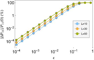
(a) Off-Diagonal Noise

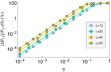
(b) Diagonal Noise

Figure 2: Relative variation of the bunching probability $P_{11}(t{=}t^{*})$ in the non-interacting regime $U_{n}{=}0$, in presence of (a) random hopping coupling strength $\epsilon$ and (b) random diagonal coupling strength $\eta$. Several chain lengths $L$ are considered.

We also consider the effect of diagonal noise $B_{j}{=}B{+}Jx_{j}$ with $x_{n}{\in}\left[-\eta,\eta\right]$ in an even site chain. The effect of signal noise is shown in figure Fig. 2(b) as function of the noise coupling strength $\epsilon$. As clear from Fig. 2(a) and 2(b) a power law behavior, under a certain threshold value of $\epsilon$ and $\eta$, characterizes both the deviations due to hopping disorder and due to the diagonal disorder. Clearly, an high degree of disorder produces state localization, which completely destroys the effect.

III.2 Quantum many-particle carpets

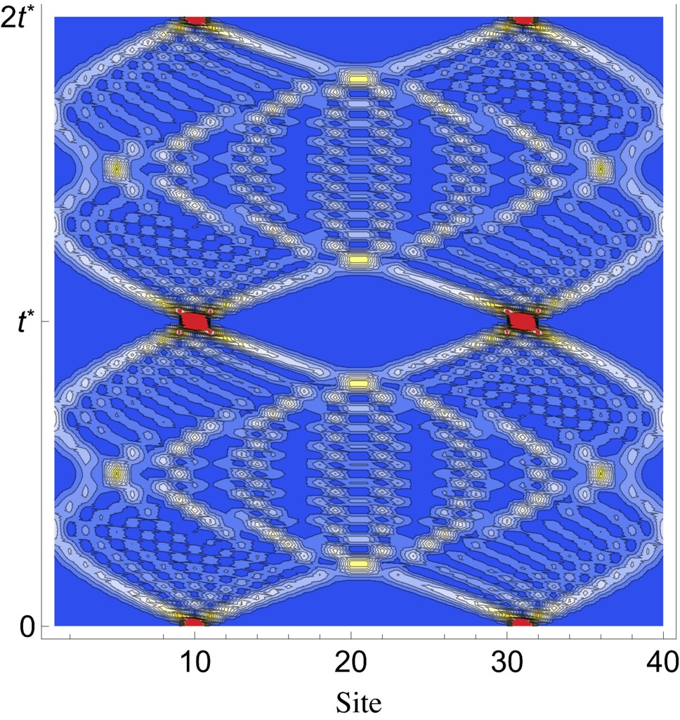
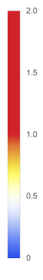
Figure 3: Quantum Carpet: space-time evolution of $\langle n_{j}^{2}(t)\rangle$ for a $L{=}40$ one-dimensional chain initialized in $|{\psi_{0}}\rangle{=}a^{\dagger}_{10}a^{\dagger}_{31}|{0}\rangle$. We consider the free-boson regime $U_{n}{=}0$. The white zones are out of the range $[0,0.4]$ which has been chosen for convenience.

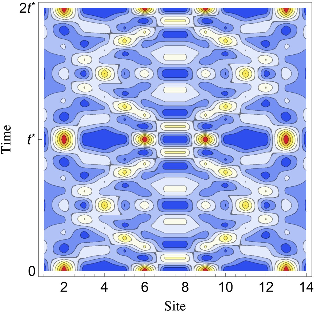
(a) $U{=}0$

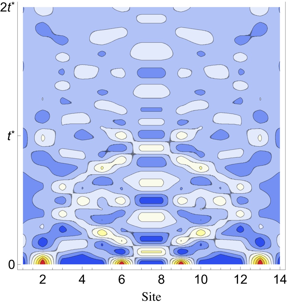
(b) $U{=}1$

(c) $U{=}30$

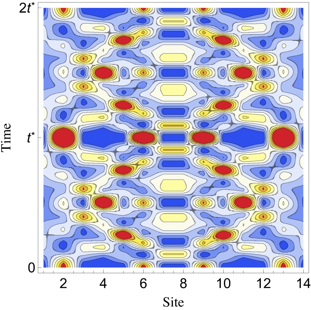
(d) $U{=}0$

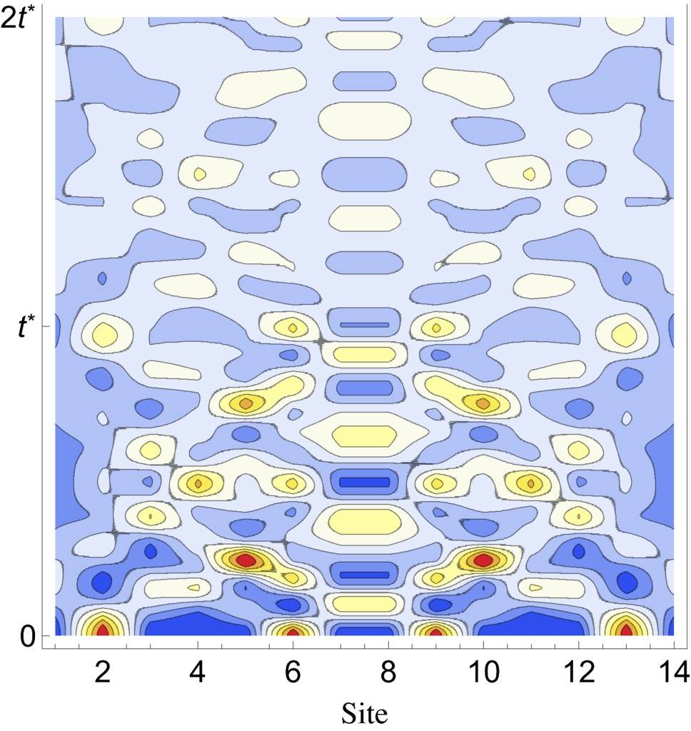
(e) $U{=}1$

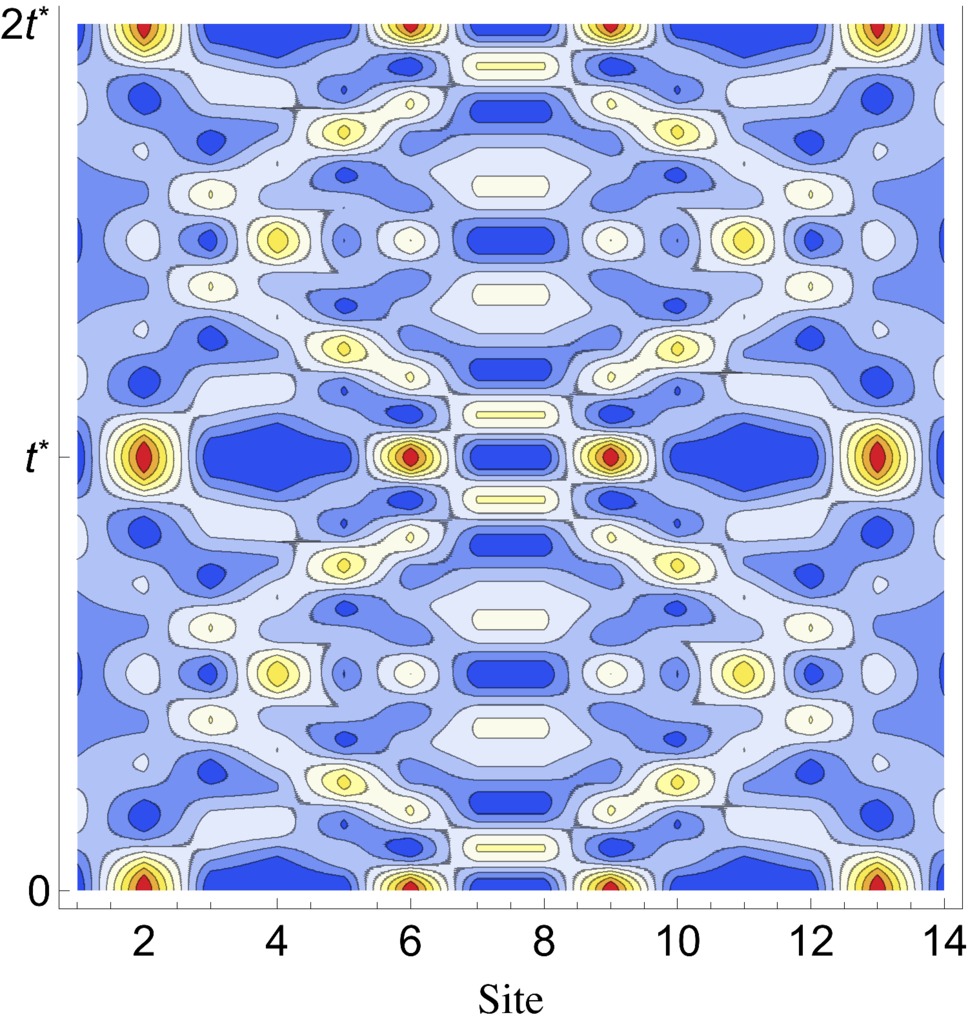
(f) $U{=}30$

Figure 4: Quantum Carpet due to four particle interference. The initial state $|{\psi_{0}}\rangle{=}a_{2}^{\dagger}a_{6}^{\dagger}a_{9}^{\dagger}a_{13}^{\dagger}|{0}\rangle$ contains four bosonic particles. We consider the space-time evolution of $\langle n_{j}(t)\rangle$ in figure (a,b,c), and the space-time evolution of $\langle n_{j}^{2}(t)\rangle$ in figures (d,e,f). The chain length is $L{=}14$ and several value of the onsite interaction $U_{n}{=}U$ are considered. Here $t^{*}$ is the fractional revival time, while $2t^{*}$ is the full revival time. The difference between the first and second row is due to bunching/anti-bunching effects. Note the transition from bosonic ($U{=}0$) to fermionic and hard-core boson ($U{=}\infty$) behavior as a function of $U$.

The perfect reconstruction scheme developed in the previous sections allows generating periodic space-time quantum interference patterns of multi-particles systems known as “quantum carpet”. By using the engineered chain with $J_{n}^{\rm split}$ and $B_{n}^{\rm split}$ one in fact expects a regular temporal pattern in the evolution: the wave-packets composing the initial state are split into two copies, reconstructed into different positions after the time $t^{*}$, and then they go back to the initial position after a time $2t^{*}$. On the other hand, during intermediate times, quantum interference leads to different behaviors which are expected to be susceptible to the particle statistics. To show this effect, we study the quantum carpet generated by the space-time evolution of the mean occupation number $\langle{n_{j}(t)}\rangle$, or by the square occupation mean $\langle{n_{j}^{2}(t)}\rangle$. The regular interference pattern of a two particle system is depicted in Fig. 3 where we show the expectation value $\langle n_{j}^{2}(t)\rangle$ for two non interacting bosons initially in $|{\psi_{0}}\rangle{=}a_{10}^{\dagger}a_{31}^{\dagger}|{0}\rangle$ in a one-dimensional chain with $L{=}40$.

To highlight more in detail the multi-particle statistical interference effect we consider a system of four particles, initially in $|{\psi_{0}}\rangle{=}a^{\dagger}_{2}a^{\dagger}_{6}a^{\dagger}_{9}a^{\dagger}_{13}|{0}\rangle$, where $L{=}14$. We show in Fig. 4(a) and 4(d) respectively the mean occupation number and the quadratic mean occupation number for the non interacting case and for the strong interacting case in Fig. 4(c) and 4(f). In the boson case bunching effects are observable at $t^{*}$ while in both cases a perfect reconstruction of the initial wavepacket happens at $2t^{*}$. This is evident more clearly in Fig. 5 where we represent the mean occupation number and the quadratic mean occupation number of site $2$ as function of time. We also take into consideration the role of the onsite interaction which affects the perfect reconstruction of a two particle wavepacket. It turns out that from the space-time dynamics of $\langle{n_{j}(t)}\rangle$ it is not possible to discriminate free evolution ($U{=}0$) from the hard-core limit ($U{=}\infty$), while particle statistics give rise to different dynamics for $\langle{n_{j}^{2}(t)}\rangle$. On the other hand, for intermediate values of the onsite interaction the dynamics does not lead to a perfect reconstruction of a wavepacket, due to scattering effects. This effect is clearly shown in Fig. 4(b), 4(e) and in Fig. 5 for $U_{n}{=}1$ where $\langle n_{2}^{2}(t{=}2t^{*})\rangle{<}\langle n_{2}^{2}(t{=}0)\rangle$ and $\langle n_{2}(t{=}2t^{*})\rangle{<}\langle n_{2}(t{=}0)\rangle$.

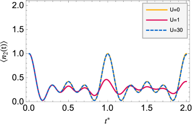
(a) Mean occupation number

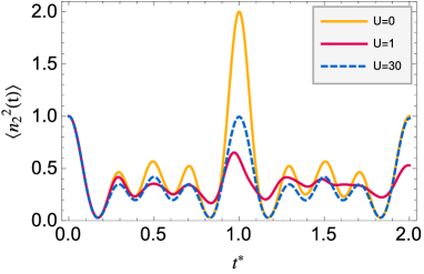
(b) Quadratic mean occupation number

Figure 5: Plot of the (a) mean occupation number and of the (b) quadratic mean occupation number of site $2$ as function of time for several values of the onsite interaction. Here $L{=}14$ and the initial state is $|{\psi(0)}\rangle{=}a_{2}^{\dagger}a_{6}^{\dagger}a_{9}^{\dagger}a_{13}^{\dagger}|{0}\rangle$. Note the transition from bosonic ($U{=}0$) to fermionic and hard-core boson ($U{=}\infty$) behavior as a function of $U$.

III.3 Perfect generation of entanglement in an XY spin chain

We now consider a chain of spin-$\frac{1}{2}$ magnets described by the XY Hamiltonian

$$\mathcal{H}=-\sum_{n}\left({J_{n}}\sigma_{n}^{+}\sigma_{n+1}^{-}+{\rm h.c.}\right)-\sum_{n}\frac{B_{n}}{2}\sigma_{n}^{z}~{},$$ (13)

where $\sigma^{\alpha}_{n}$, $\alpha{=}x,y,z$ are the Pauli spin operators acting on the spin localized in the $n$-th site of the chain, and $\sigma^{\pm}_{n}{=}(\sigma^{x}_{n}{\pm}i\sigma^{y}_{n}){/}2$. Effective spin-$\frac{1}{2}$ systems coupled by the Hamiltonian (13) with site dependent coupling strengths can be obtained in different physical realizations; e.g. in NRM using global rotations and suitable field gradients Ajoy and Cappellaro (2013), with atomic ions confined in segmented microtraps Wunderlich et al. (2009), with neutral atoms trapped into an optical lattice by polarized laser beams Duan et al. (2003); Fukuhara et al. (2013b), or with superconducting qubits coupled either by site dependent capacitors Neeley et al. (2010) or inductors Chen et al. (2014).

The system Hamiltonian (13) can be mapped to a fermionic hopping model via the Jordan-Wigner transformation: the operators $c_{n}{=}\prod_{j<n}(-\sigma^{z}_{j})\sigma_{n}^{-}$ satisfy canonical anticommutation relations and $\mathcal{H}{=}\sum_{nm}\langle{n}|H|{m}\rangle\;c_{n}^{\dagger}c_{m}$  , where $H$ is the hopping matrix (1). Every many-body spin state can be obtained by applying the annihilation operators $c_{n}$ to the fully polarized state $|{\Omega}\rangle{=}|{\uparrow\uparrow\cdots}\rangle$. Therefore, the time evolution of a generic initial state can be obtained by expressing the operator $c_{n}$ in the Heisenberg picture Banchi (2013) as

$$c_{n}(t)=\sum_{m}\langle{n}|e^{-iHt}|{m}\rangle\;c_{m}.$$ (14)

We now show how one can create entanglement between two remote mirror symmetric sites by exploiting the perfect wave-packet splitting (7). Suppose that, starting from the fully polarized state $|{\Omega}\rangle$ a particle is flipped in position $n$; the initial state of the system is then $c_{n}|{\Omega}\rangle$. When the single-particle Hamiltonian implements the transformation (7), then, thanks to Eq.(14) one has $c_{n}|{\Omega}\rangle\xrightarrow{t^{*}}(c_{n}|{\Omega}\rangle{+}ic_{L-n+1}|{\Omega}\rangle)/\sqrt{2}$. Therefore, going back to the spin picture, after the time $t^{*}$ an entangled state $\frac{|{\uparrow\downarrow}\rangle+i|{\downarrow\uparrow}\rangle}{\sqrt{2}}$ between sites $n$ and $L{-}n{+}1$ is generated.

The above arguments can be generalized in a many-particle setting to generate the maximal amount of entangled pairs starting from a separable state. Two suitable choices of the initial state are

$$|{\psi^{\rm DM}}\rangle =|{\uparrow\uparrow\cdots\uparrow\downarrow\cdots\downarrow\downarrow}\rangle~{},$$ (15)

$$|{\psi^{\rm AFM}}\rangle =|{\uparrow\downarrow\uparrow\cdots\uparrow\downarrow}\rangle~{},$$ (16)

namely the domain-wall state $|{\psi^{\rm DM}}\rangle$ or the anti-ferromagnetic state $|{\psi^{\rm AFM}}\rangle$. If the system is initialized in either $|{\psi^{\rm DM}}\rangle$ or $|{\psi^{\rm AFM}}\rangle$ and is let to evolve under the perfect splitting Hamiltonian, then the resulting state after a time $t^{*}$ is $(c_{1}+e^{i\alpha_{1}}c_{L})(c_{2}+e^{i\alpha_{2}}c_{L-1})(c_{3}+e^{i\alpha_{2}}c_{L-2})\cdots|{\Omega}\rangle$, where $\alpha_{i}$ depends on the initial state. By carefully dealing with the Jordan-Wigner phase entering into the definition of the operators $c_{n}$ one can easily find that the resulting state corresponds to a state in which every pair of qubits sitting in positions $n$ and $L{-}n{+}1$ is maximally entangled. The perfect splitting dynamics thus represents an alternative to other methods existing in the literature to generate nested Bell pairs Di Franco et al. (2008); Alkurtass et al. (2014) starting from a separable state. However, compared to previous proposals it is more general because it allows tuning the number of generated Bell pairs by simply choosing the number of flipped spins in the initial state.

IV Conclusions

In this paper we study the wavefunction dynamics of hopping particles and/or quasi-particles in a quantum chain. We design the Hamiltonian so that a localized wave packet evolves coherently along the chain without dispersion, and at particular point is perfectly split into transmitted and reflected components which propagate in opposite directions without dispersion. When the reflected component reaches the initial site, its wave packet becomes localized while, at the same time, the wave packet of the transmitted component becomes localized in a different site of the chain. We devise the exact conditions that the Hamiltonian spectrum has to satisfy to allow for the perfect splitting and reconstruction. Then we focus on some viable Hamiltonians with nearest-neighbor interactions and site-dependent couplings, and we find the coupling pattern which satisfies the perfect splitting condition using inverse eigenvalue techniques.

Besides shedding new light into quantum interference phenomena in one dimension, our results are particularly useful for applications. In this respect, we study atomic lattices and obtain perfect Hanbury Brown and Twiss correlations and peculiar quantum interference patterns which result in regular structure in the space-time evolution of the many-particle wave function. Moreover, we show that in a spin chain setting, the particle splitting can be used to generate maximally entangled states between distant parts.

We expect that the perfect wavepacket splitting will become a general tool for varied applications in controlled quantum interference and quantum information processing.

V Acknowledgments

The authors acknowledge the financial support by the ERC under Starting Grant 308253 PACOMANEDIA.

Appendix A Perfect splitting Hamiltonian for $L=5,6$

The Hamiltonian matrices $\langle{n}|H|{m}\rangle$ for perfect balanced splitting when $L{=}5$ and $6$ are respectively (in unit of $J$):

$$\left(\begin{array}[]{ccccc}-0.08378&0.6195&0&0&0\\ 0.6195&-0.2932&0.6664&0&0\\ 0&0.6664&0.7540&0.6664&0\\ 0&0&0.6664&-0.2932&0.6195\\ 0&0&0&0.6195&-0.08378\\ \end{array}\right)$$

$$\left(\begin{array}[]{cccccc}0&0.5999&0&0&0&0\\ 0.5999&0&0.8279&0&0&0\\ 0&0.8279&0&0.3927&0&0\\ 0&0&0.3927&0&0.8279&0\\ 0&0&0&0.8279&0&0.5999\\ 0&0&0&0&0.5999&0\\ \end{array}\right)~{}.$$

As shown in Section III, small imperfections parameter tuning result in negligible deviations from the ideal dynamics.

References

- Preiss et al. (2014) P. M. Preiss, R. Ma, M. E. Tai, A. Lukin, M. Rispoli, P. Zupancic, Y. Lahini, R. Islam, and M. Greiner, arXiv:1409.3100 [cond-mat] (2014).
- Fukuhara et al. (2013a) T. Fukuhara, A. Kantian, M. Endres, M. Cheneau, P. Schauß, S. Hild, D. Bellem, U. Schollwöck, T. Giamarchi, C. Gross, I. Bloch, and S. Kuhr, Nat Phys 9, 235 (2013a).
- Fukuhara et al. (2013b) T. Fukuhara, P. Schauß, M. Endres, S. Hild, M. Cheneau, I. Bloch, and C. Gross, Nature 502, 76 (2013b).
- Sansoni et al. (2012) L. Sansoni, F. Sciarrino, G. Vallone, P. Mataloni, A. Crespi, R. Ramponi, and R. Osellame, Phys. Rev. Lett. 108, 010502 (2012).
- Ramanathan et al. (2011) C. Ramanathan, P. Cappellaro, L. Viola, and D. G. Cory, New J. Phys. 13, 103015 (2011).
- Schreiber et al. (2015) M. Schreiber, S. S. Hodgman, P. Bordia, H. P. Lüschen, M. H. Fischer, R. Vosk, E. Altman, U. Schneider, and I. Bloch, arXiv:1501.05661 [cond-mat, physics:quant-ph] (2015).
- Richerme et al. (2014) P. Richerme, Z.-X. Gong, A. Lee, C. Senko, J. Smith, M. Foss-Feig, S. Michalakis, A. V. Gorshkov, and C. Monroe, Nature 511, 198 (2014).
- Schachenmayer et al. (2013) J. Schachenmayer, B. Lanyon, C. Roos, and A. Daley, Physical Review X 3, 031015 (2013).
- Trompeter et al. (2006) H. Trompeter, T. Pertsch, F. Lederer, D. Michaelis, U. Streppel, A. Bräuer, and U. Peschel, Phys. Rev. Lett. 96, 023901 (2006).
- Kaplan et al. (2000) A. E. Kaplan, I. Marzoli, W. E. Lamb, and W. P. Schleich, Phys. Rev. A 61, 032101 (2000).
- Robinett (2004) R. W. Robinett, Physics Reports 392, 1 (2004).
- Berry et al. (2001) M. Berry, I. Marzoli, and W. Schleich, Phys. World 14, 39 (2001).
- Kempe (2003) J. Kempe, Contemporary Physics 44, 307 (2003).
- Childs (2009) A. M. Childs, Phys. Rev. Lett. 102, 180501 (2009).
- Childs et al. (2003) A. M. Childs, R. Cleve, E. Deotto, E. Farhi, S. Gutmann, and D. A. Spielman, in Proceedings of the Thirty-fifth Annual ACM Symposium on Theory of Computing, STOC ’03 (ACM, New York, NY, USA, 2003) pp. 59–68.
- Longhi (2010) S. Longhi, Phys. Rev. B 82, 041106 (2010).
- Cirac et al. (1997) J. I. Cirac, P. Zoller, H. J. Kimble, and H. Mabuchi, Phys. Rev. Lett. 78, 3221 (1997).
- Ritter et al. (2012) S. Ritter, C. Nölleke, C. Hahn, A. Reiserer, A. Neuzner, M. Uphoff, M. Mücke, E. Figueroa, J. Bochmann, and G. Rempe, Nature 484, 195 (2012).
- Bose (2007) S. Bose, Contemporary Physics 48, 13 (2007).
- Nikolopoulos and Jex (2013) G. M. Nikolopoulos and I. Jex, eds., Quantum State Transfer and Network Engineering, 2014th ed. (Springer, New York, 2013).
- Aronstein and Stroud (1997) D. L. Aronstein and C. R. Stroud, Phys. Rev. A 55, 4526 (1997).
- Kay (2010) A. Kay, Int. J. Quantum Inform. 08, 641 (2010).
- Albanese et al. (2004) C. Albanese, M. Christandl, N. Datta, and A. Ekert, Phys. Rev. Lett. 93, 230502 (2004).
- Yung and Bose (2005) M.-H. Yung and S. Bose, Phys. Rev. A 71, 032310 (2005).
- Godsil et al. (2012) C. Godsil, S. Kirkland, S. Severini, and J. Smith, Phys. Rev. Lett. 109, 050502 (2012).
- Banchi (2013) L. Banchi, Eur. Phys. J. Plus 128, 1 (2013).
- Banchi et al. (2011) L. Banchi, T. J. G. Apollaro, A. Cuccoli, R. Vaia, and P. Verrucchi, New J. Phys. 13, 123006 (2011).
- Yao et al. (2011) N. Y. Yao, L. Jiang, A. V. Gorshkov, Z.-X. Gong, A. Zhai, L.-M. Duan, and M. D. Lukin, Phys. Rev. Lett. 106, 040505 (2011).
- Chen et al. (2007) B. Chen, Z. Song, and C. P. Sun, Phys. Rev. A 75, 012113 (2007).
- Compagno et al. (2014) E. Compagno, L. Banchi, and S. Bose, arXiv:1407.8501 [quant-ph] (2014).
- Fogarty et al. (2013) T. Fogarty, A. Kiely, S. Campbell, and T. Busch, Phys. Rev. A 87, 043630 (2013).
- Gertjerenken (2013) B. Gertjerenken, Phys. Rev. A 88, 053623 (2013).
- Makin et al. (2012) M. I. Makin, J. H. Cole, C. D. Hill, and A. D. Greentree, Phys. Rev. Lett. 108, 017207 (2012).
- Brown and Twiss (1956) R. H. Brown and R. Q. Twiss, Nature 177, 27 (1956).
- Mitra (2015) C. Mitra, Nat Phys advance online publication (2015), 10.1038/nphys3249.
- Sahling et al. (2015) S. Sahling, G. Remenyi, C. Paulsen, P. Monceau, V. Saligrama, C. Marin, A. Revcolevschi, L. P. Regnault, S. Raymond, and J. E. Lorenzo, Nat Phys advance online publication (2015), 10.1038/nphys3186.
- Alkurtass et al. (2014) B. Alkurtass, L. Banchi, and S. Bose, Phys. Rev. A 90, 042304 (2014).
- Di Franco et al. (2008) C. Di Franco, M. Paternostro, and M. S. Kim, Phys. Rev. A 77, 020303 (2008).
- Christandl et al. (2004) M. Christandl, N. Datta, A. Ekert, and A. J. Landahl, Phys. Rev. Lett. 92, 187902 (2004).
- Kay (2006) A. Kay, Phys. Rev. A 73, 032306 (2006).
- Bruderer et al. (2012) M. Bruderer, K. Franke, S. Ragg, W. Belzig, and D. Obreschkow, Phys. Rev. A 85, 022312 (2012).
- Parlett (1998) B. Parlett, The Symmetric Eigenvalue Problem, Classics in Applied Mathematics (Society for Industrial and Applied Mathematics, 1998).
- Chu (1998) M. Chu, SIAM Rev. 40, 1 (1998).
- Friedland et al. (1987) S. Friedland, J. Nocedal, and M. L. Overton, SIAM Journal on Numerical Analysis 24, 634 (1987).
- Jaksch et al. (1998) D. Jaksch, C. Bruder, J. I. Cirac, C. W. Gardiner, and P. Zoller, Phys. Rev. Lett. 81, 3108 (1998).
- Greiner et al. (2002) M. Greiner, O. Mandel, T. Esslinger, T. W. Hänsch, and I. Bloch, Nature 415, 39 (2002).
- Jördens et al. (2008) R. Jördens, N. Strohmaier, K. Günter, H. Moritz, and T. Esslinger, Nature 455, 204 (2008).
- Modugno et al. (2003) G. Modugno, F. Ferlaino, R. Heidemann, G. Roati, and M. Inguscio, Phys. Rev. A 68, 011601 (2003).
- Rigol and Muramatsu (2004) M. Rigol and A. Muramatsu, Phys. Rev. A 70, 031603 (2004).
- Wang et al. (2013) Z.-M. Wang, L.-A. Wu, M. Modugno, W. Yao, and B. Shao, Sci Rep 3 (2013), 10.1038/srep03128.
- Bakr et al. (2009) W. S. Bakr, J. I. Gillen, A. Peng, S. Fölling, and M. Greiner, Nature 462, 74 (2009).
- Boyer et al. (2006) V. Boyer, R. M. Godun, G. Smirne, D. Cassettari, C. M. Chandrashekar, A. B. Deb, Z. J. Laczik, and C. J. Foot, Phys. Rev. A 73, 031402 (2006).
- Weitenberg et al. (2011) C. Weitenberg, M. Endres, J. F. Sherson, M. Cheneau, P. Schauß, T. Fukuhara, I. Bloch, and S. Kuhr, Nature 471, 319 (2011).
- Endres et al. (2013) M. Endres, M. Cheneau, T. Fukuhara, C. Weitenberg, P. Schauß, C. Gross, L. Mazza, M. C. Bañuls, L. Pollet, I. Bloch, and S. Kuhr, Appl. Phys. B 113, 27 (2013).
- Gross and Bloch (2014) C. Gross and I. Bloch, arXiv:1409.8501 [cond-mat] (2014).
- Sanders et al. (2011) J. C. Sanders, O. Odong, J. Javanainen, and M. Mackie, Phys. Rev. A 83, 031607 (2011).
- Meinert et al. (2014) F. Meinert, M. J. Mark, E. Kirilov, K. Lauber, P. Weinmann, M. Gröbner, and H.-C. Nägerl, Phys. Rev. Lett. 112, 193003 (2014).
- Hong et al. (1987) C. K. Hong, Z. Y. Ou, and L. Mandel, Phys. Rev. Lett. 59, 2044 (1987).
- Kaufman et al. (2014) A. M. Kaufman, B. J. Lester, C. M. Reynolds, M. L. Wall, M. Foss-Feig, K. R. A. Hazzard, A. M. Rey, and C. A. Regal, Science 345, 306 (2014).
- Keating et al. (2007) J. P. Keating, N. Linden, J. C. F. Matthews, and A. Winter, Phys. Rev. A 76, 012315 (2007).
- Stasińska et al. (2014) J. Stasińska, M. Łącki, O. Dutta, J. Zakrzewski, and M. Lewenstein, Physical Review A 90 (2014).
- Ospelkaus et al. (2006) S. Ospelkaus, C. Ospelkaus, O. Wille, M. Succo, P. Ernst, K. Sengstock, and K. Bongs, Phys. Rev. Lett. 96, 180403 (2006).
- Zwick et al. (2011) A. Zwick, G. A. Álvarez, J. Stolze, and O. Osenda, Phys. Rev. A 84, 022311 (2011).
- Ajoy and Cappellaro (2013) A. Ajoy and P. Cappellaro, Phys. Rev. Lett. 110, 220503 (2013).
- Wunderlich et al. (2009) H. Wunderlich, C. Wunderlich, K. Singer, and F. Schmidt-Kaler, Phys. Rev. A 79, 052324 (2009).
- Duan et al. (2003) L.-M. Duan, E. Demler, and M. D. Lukin, Phys. Rev. Lett. 91, 090402 (2003).
- Neeley et al. (2010) M. Neeley, R. C. Bialczak, M. Lenander, E. Lucero, M. Mariantoni, A. D. O’Connell, D. Sank, H. Wang, M. Weides, J. Wenner, Y. Yin, T. Yamamoto, A. N. Cleland, and J. M. Martinis, Nature 467, 570 (2010).
- Chen et al. (2014) Y. Chen, C. Neill, P. Roushan, N. Leung, M. Fang, R. Barends, J. Kelly, B. Campbell, Z. Chen, B. Chiaro, A. Dunsworth, E. Jeffrey, A. Megrant, J. Y. Mutus, P. J. J. O’Malley, C. M. Quintana, D. Sank, A. Vainsencher, J. Wenner, T. C. White, M. R. Geller, A. N. Cleland, and J. M. Martinis, Phys. Rev. Lett. 113, 220502 (2014).