Gamma-ray burst spectra and spectral correlations from sub-photospheric Comptonization

Abstract

One of the most important unresolved issues in gamma-ray burst physics is the origin of the prompt gamma-ray spectrum. Its general non-thermal character and the softness in the X-ray band remain unexplained. We tackle these issues by performing Monte Carlo simulations of radiation-matter interactions in a scattering dominated photon-lepton plasma. The plasma – initially in equilibrium – is driven to non-equilibrium conditions by a sudden energy injection in the lepton population, mimicking the effect of a shock wave or the dissipation of magnetic energy. Equilibrium restoration occurs due to energy exchange between the photons and leptons. While the initial and final equilibrium spectra are thermal, the transitional photon spectra are characterized by non-thermal features such as power-law tails, high energy bumps, and multiple components. Such non-thermal features are observed at infinity if the dissipation occurs at small to moderate optical depths, and the spectrum is released before thermalization is complete. We model the synthetic spectra with a Band function and show that the resulting spectral parameters are similar to observations for a frequency range of 2-3 orders of magnitude around the peak. In addition, our model predicts correlations between the low-frequency photon index and the peak frequency as well as between the low- and high-frequency indices. We explore baryon and pair dominated fireballs and reach the conclusion that baryonic fireballs are a better model for explaining the observed features of gamma-ray burst spectra.

1. Introduction

The radiation mechanism that produces the bulk of the prompt emission of Gamma-Ray Bursts (GRBs) is still a matter of open debate (e.g. Mastichiadis & Kazanas 2009; Medvedev et al. 2009; Ryde & Pe’er 2009; Asano et al. 2010; Ghisellini 2010; Lazzati & Begelman 2010; Daigne et al. 2011; Massaro & Grindlay 2011; Resmi & Zhang 2012; Hascoët et al. 2013; Crumley & Kumar 2013). Among the many proposed possibilities, the synchrotron shock model (SSM) and the photospheric model (PhM) have recently gathered most of the attention (Rees & Meszaros 1994; Piran 1999; Lloyd & Petrosian 2000; Mészáros & Rees 2000; Rees & Mészáros 2005; Giannios 2006; Pe’er et al. 2006; Bošnjak et al. 2009; Lazzati et al. 2009; Beloborodov 2010; Mizuta et al. 2011; Nagakura et al. 2011). Within the SSM, the bulk of the prompt radiation is produced by synchrotron from a non-thermal population of electrons gyrating around a strong, locally-generated magnetic field. The non-thermal leptons are produced either by trans-relativistic internal shocks (the SSM proper, Rees & Meszaros 1994) or by magnetic reconnection in a Poynting flux dominated outflow (e.g. the ICMART model, Zhang & Yan 2011). The SSM naturally accounts for the broad, non-thermal nature of the spectrum. However, it has difficulties in accounting for bursts with particularly steep low-frequency slopes (Preece et al. 1998; Ghisellini et al. 2000) and has limited predictive power, since the radiation properties are tied to poorly constrained quantities such as the lepton’s energy distribution, the ad-hoc equipartition parameters, and the ejection history of shells from the central engine.

The PhM does not specify a radiation mechanism, assuming instead that the burst radiation is produced in the optically thick part of the outflow and advected out, its spectrum being the result of the strain between mechanisms that tend to bring radiation and plasma in thermal equilibrium and mechanisms that can bring them out of balance (e.g., Beloborodov 2013). The PhM has been shown to be able to reproduce ensemble properties of the GRB population, such as the debated Amati correlation, the Golenetskii correlation, and the recently discovered correlation between the burst energetics and the Lorentz factor of the outflow (Amati et al. 2002; Amati 2006; Liang et al. 2010; Fan et al. 2012; Ghirlanda et al. 2012; Lazzati et al. 2013; López-Cámara et al. 2014). However, it is not yet understood how the broad-band nature of the prompt spectrum, spanning many orders of magnitude in frequency, is produced. In a hot, dissipationless flow, only the adiabatic cooling of the plasma would work as a mechanism to break equilibrium, and the GRB outflow would work as a miniature big bang, the entrained radiation maintaining a Planck spectrum. In a cold, dissipationless outflow, lepton scattering dominates the radiation-matter interaction producing a Wien spectrum (Rybicki & Lightman 1979). Outflows from GRB progenitors are, however, far from dissipationless. Hydrodynamic outflows are continuously shocked out to large radii (Lazzati et al. 2009), and Poynting-dominated outflows suffer dissipation through magnetic reconnection (Giannios & Spruit 2006). Either way, even if thermal equilibrium is reached at some point in the outflow, it is likely that such equilibrium is broken by a sudden release of energy in the lepton population or altered by a slow and continuous (or episodic) injection of energy. The effects of such energy injection on the photospheric spectrum are profound (e.g., Giannios 2006; Pe’er et al. 2006; Beloborodov 2010; Lazzati & Begelman 2010). In addition, the interaction between different parts of the outflow in a stratified flow alter the thermal spectra into a non-thermal, highly polarized spectrum (Ito et al. 2013, 2014; Lundman et al. 2013).

In this paper we investigate the evolution of the radiation spectrum following the sudden injection of energy in the lepton population of a plasma, assuming that the radiation and leptons interact via Compton scattering and pair processes. We use a Monte Carlo (MC) method that evolves simultaneously the photon and lepton populations by performing inelastic scattering between photons and leptons in both the non-relativistic and the relativistic (Klein-Nishina) regimes. The code also accounts for $e^{-}e^{+}$ annihilation (pair annihilation henceforth) and $e^{-}e^{+}$ pair production from photon-photon collisions (pair production henceforth). We focus on transient features that can be observed if the episode(s) of energy injection in the leptons occur at small or moderate optical depths ($\tau<1000$).

This manuscript is organized as follows. In Section 2 we describe the physics and the methods of the MC code, in Section 3 we show our results and in Section 4 we discuss the results and compare them to previous findings.

2. Methodology

2.1. Step 1: Particle Generation

As a first task, the code generates a user-defined number of leptons and photons. Their energies follow a distribution that can be either of thermal equilibrium (Wien for the photons and Maxwell-Jüttner for the leptons) or any other user-specified distribution. After initializing the photon and lepton distributions, our code performs the following steps iteratively.

2.2. Step 2: Particle/Process selection

To initiate either a scattering or a pair event we need to select two particles - which we obtain by randomly selecting a pair from our generated distributions. Depending upon the particles selected, Compton scattering (if a photon and a lepton is chosen), pair annihilation (if an $e^{-}$ or $e^{+}$ is chosen) or pair production (if two photons are chosen) is performed or another pair is re-selected if any other combination occurs. After the selection, the code proceeds with the following calculations:

• Incident angle generation ($\theta$) using the appropriate relativistic scattering rates, under the assumption that both leptons and photons are isotropically distributed.

• Lorentz boost to the necessary reference frames (details explained in successive sections) from the lab frame.

• Event probability computations from total cross section ($\sigma$) calculations.

• Scattering angle generation from differential cross section ($\frac{d\sigma}{d\Omega}$).

• Lorentz boost from the necessary frame back to the lab frame.

In the following sub-sections we discuss each of the three possible processes in detail

2.2.1 Process 1: Compton Scattering

As the choice of reference frame is arbitrary, in the lab frame we can assume that the lepton is traveling along the x-axis and the photon is incident upon the lepton in the xy plane without any loss of generality. The angle of incidence $\theta_{\gamma e}$ between the chosen photon-lepton pair is generated by a probability distribution $P_{\gamma e}$:

$$P_{\gamma e}(\beta_{e},\theta_{\gamma e})\propto\sin\theta_{\gamma e}(1-\beta_{e}\cos\theta_{\gamma e})$$ (1)

where $\beta_{e}=v_{e}/c$, is the ratio of lepton speed to the speed of light.
To simulate the scattering event the code Lorentz transforms to the lepton frame (that we call the co-moving frame). The probability that the chosen photon-lepton pair interacts depends on the incident photon energy in the co-moving frame. As Compton scattering becomes less efficient at higher energies, photons having energies comparable to or greater than the lepton’s rest mass energy are less likely to scatter. Using Monte Carlo sampling we determine if scattering occurs or not. This is done by generating a random number and comparing it to the ratio of the Klein-Nishina cross section $\sigma_{\gamma e}$ to the Thomson cross section, which we use as a reference value. We proceed with the scattering event if $\sigma_{\gamma e}/\sigma_{T}\geq s_{1}$ where $s_{1}$ is a random number. If the condition is not satisfied, the code returns to step 2. If instead the condition is satisfied and the scattering occurs, the code generates the polar scattering angle $\theta^{\prime}_{s}$ in accordance with the Klein-Nishina differential cross-section formula

$$\frac{d\sigma_{\gamma e}}{d\Omega}=\frac{r^{2}_{0}}{2}\frac{E_{s}^{\prime 2}}{E^{\prime 2}}\left(\frac{E^{\prime}}{E^{\prime}_{s}}+\frac{E^{\prime}_{s}}{E^{\prime}}-\sin^{2}\theta^{\prime}_{s}\right)$$ (2)

where $r_{0}$ is the classical radius of an electron, $E^{\prime}$ and $E^{\prime}_{s}$ are the energies of the incident and scattered photon respectively (e.g. Bluementhal & Gould 1970, Longair 2003 and Rybicki & Lightman 1979). The energy transfer equation connecting $E^{\prime}$ with $E^{\prime}_{s}$ is the Compton equation (e.g. Bluementhal & Gould 1970, Longair 2003 and Rybicki & Lightman 1979)

$$E^{\prime}_{s}=\frac{E^{\prime}}{1+\frac{E^{\prime}}{m_{e}c^{2}}(1-\cos\theta^{\prime}_{s})}.$$ (3)

(Note here that $\theta^{\prime}_{s}$ is the angle that the scattered photon makes with the direction of propagation of the incident photon in the co-moving frame. Hence equations (2) and (3) hold true only in the lepton frame). Finally, the azimuthal angle $\phi^{\prime}_{s}$ is generated randomly between zero and $2\pi$. Thus, we now have the four momenta of the scattered particles in the co-moving frame.

2.2.2 Process 2: Pair Production / Photon Annihilation

If the particle selection process selects two photons then the pair production/photon annihilation channel is chosen. The code computes the angle of incidence $\theta_{\gamma\gamma}$ between the chosen photons by using the probability distribution $P_{\gamma\gamma}$:

$$P_{\gamma\gamma}(\theta_{\gamma\gamma})\propto\sin{\theta_{\gamma\gamma}}(1-\cos{\theta_{\gamma\gamma}}).$$ (4)

To ensure that the photon pair has enough energy to lead to a pair production event the code checks the energy of the photon/s in the zero momentum frame. The zero momentum frame photon energy $E^{\prime}_{o}$ can be computed given the incident photon energies $E_{1}$, $E_{2}$ and the incident angle as

$$E^{\prime}_{o}=\sqrt{E_{1}E_{2}}\sin(\theta_{\gamma\gamma}/2).$$ (5)

(Gould & Schereder 1967). If $E^{\prime}_{o}<m_{e}c^{2}$ the colliding photon pair is not energetic energy to produce an $e^{-}e^{+}$ pair, hence the code jumps to step 2 for a new particle pair selection. Due to the energy dependence of cross-section $\sigma_{\gamma\gamma}$, even photons exceeding the energy threshold might not produce pairs. To make this determination, we again use the Thomson cross section as a reference and determine if the photon annihilation takes place by randomly drawing one number $s_{2}$, obtaining $\sigma_{\gamma\gamma}$ by boosting to the center of momentum frame and evaluating if $\sigma_{\gamma\gamma}/\sigma_{T}\geq s_{2}$. If the inequality holds true, the code proceeds with the pair production calculation. Otherwise, it is abandoned and the code returns to step 2.
Once the photons succeed in producing leptons, the polar scattering angle $\theta^{\prime}_{s}$ of the newly born $e^{-}$ is computed from the pair annihilation differential cross section as given by

$$\frac{d\sigma_{{\gamma\gamma}}}{d\Omega}=\frac{r_{0}^{2}\pi}{2}b\left(\frac{m_{e}c^{2}}{E^{\prime}_{o}}\right)^{2}\frac{1-b^{4}\cos^{4}{\theta^{\prime}_{s}}+2\left(\frac{m_{e}c^{2}}{E^{\prime}_{o}}\right)^{2}b^{2}\sin^{2}{\theta^{\prime}_{s}}}{\left(1-b^{2}\cos^{2}{\theta^{\prime}_{s}}\right)^{2}}.$$ (6)

(see Jauch & Rohrlich 1980, p.300) where $b=\sqrt{1-\left(\frac{m_{e}c^{2}}{E^{\prime}_{o}}\right)^{2}}$. A random azimuthal angle $\phi^{\prime}_{s}\in[0,2\pi)$ is assigned to the $e^{-}$. Note that Lorentz transformation to the zero momentum frame is necessary because equation (6) is frame dependent. Utilizing conservation laws, the four momenta of the $e^{+}$ can be determined.

2.2.3 Process 3: Pair Annihilation/ Photon Production

The pair annihilation channel is chosen if the random particle selection constitutes an $e^{-}e^{+}$ pair. As with the other channels, we first determine the incident angle $\theta_{ee}$ (subscript _ee stands for lepton pair annihilation) between the pair by computing the probability distribution of scattering as given by

$$P_{ee}(\beta_{e^{-}},\beta_{e^{+}},\theta_{ee})\propto\sin{\theta_{ee}}f_{kin}$$ (7)

where $f_{kin}$ as obtained from (Coppi & Blandford 1990) is given by:

$$f_{kin}=\sqrt{\beta_{e^{-}}^{2}+\beta_{e^{+}}^{2}-\beta_{e^{-}}^{2}\beta_{e^{+}}^{2}\sin^{2}{\theta_{ee}}-2\beta_{e^{-}}\beta_{e^{+}}\cos{\theta_{ee}}}.$$ (8)

Here $\beta_{e}=\frac{v_{e}}{c}$ i.e. the ratio of lepton speed to the speed of light. The code transforms all quantities to the rest frame of the electron to calculate the the total cross section $\sigma_{ee}$ as (Jauch & Rohrlich 1980, p.269):

$$\sigma_{ee}=\frac{r_{0}^{2}\pi}{\beta^{\prime 2}}\left[\frac{\left(\gamma^{\prime}+\frac{1}{\gamma^{\prime}}+4\right)\ln{(\gamma^{\prime}+\sqrt{\gamma^{\prime 2}-1}})-\beta^{\prime}(\gamma^{\prime}+3)}{\gamma^{\prime}(\gamma^{\prime}+1)}\right]$$ (9)

where $\beta^{\prime}=v^{\prime}_{e+}/c$, $\gamma^{\prime}=\frac{1}{\sqrt{1-\beta^{\prime 2}}}$ i.e. the $e^{+}$ speed and Lorentz factor respectively in the co-moving frame traveling with the $e^{-}$. On comparing the $\sigma_{ee}/\sigma_{T}$ with a random number $s_{3}$ the code evaluates the occurrence of the annihilation event. If the event fails, the code returns to step 2 to re-select another pair of particles. Following a successful event, the polar scattering angle $\theta^{\prime}_{s}$ between either of the pair produced photons is generated from the differential cross section (from Jauch & Rohrlich 1980, p.268)

$$\frac{d\sigma_{ee}}{d\Omega}=\frac{r_{0}^{2}\pi}{\beta^{\prime}\gamma^{\prime}d}\left[\gamma^{\prime}+3-\frac{\left[1+d\right]^{2}}{(1+\gamma^{\prime})d}-\frac{2(1+\gamma^{\prime})d}{\left[1+d\right]^{2}}\right]$$ (10)

where $x=\cos{\theta^{\prime}_{s}}$ and $d=\gamma^{\prime}(1-\beta^{\prime}x)$. As pointed out in the preceding sub-sections, Lorentz transformation to the electron frame is necessary as equation (10) is expressed in terms of quantities defined in the electron’s co-moving frame. The random azimuthal angle $\phi^{\prime}_{s}\in[0,2\pi)$ is randomly assigned to either photon. Using conservation laws, the four momenta of the pair produced photons can be obtained.

2.3. Step 3: Back to the lab frame

At the end of the event, the code transforms the four momenta of the particles back to the lab frame by employing Lorentz transformations. The loop is repeated until equilibrium is restored i.e. when the particle numbers saturate and distributions become thermal.

3. Results

We employ the Monte Carlo code described above to study the evolution of the radiation spectrum in a closed box containing leptons and photons. The simulations are initialized with a Wien radiation spectrum at $10^{6}$ K and a non-equilibrium lepton population, either because leptons and photons are at different temperature or because the leptons energy distribution is non-thermal. This is expected to mimic a scenario in which the leptons and radiation were initially at equilibrium, but the lepton population has been brought out of equilibrium by a sudden energy release. Such energy release may be due to shocks in the fluid (e.g., Rees & Meszaros 1994; Lazzati & Begelman 2010) or by magnetic reconnection in a magnetized outflow (e.g. Giannios & Spruit 2006, McKinney & Uzdensky 2012). As it will be clear at the end, a fundamental parameter that determines the interaction between the photons and leptons is the particle ratio, i.e., the ratio of photon and lepton number densities. In a GRB outflow, such a ratio can be readily estimated.

Let us call $E_{K}$ the kinetic energy of the outflow carried by particles with non-zero rest mass and $E_{\gamma}$ the energy in electromagnetic radiation. We have:

$$\frac{E_{\gamma}}{E_{K}} = \frac{N_{\gamma}h\nu_{\rm{pk}}}{\left(N_{p}+\frac{m_{e}}{m_{p}}N_{\rm{lep}}\right)\Gamma m_{p}c^{2}}$$ (11)

$$\simeq 10^{-5}\frac{n_{\gamma}}{n_{p}+\frac{n_{\rm{lep}}}{1836}}\left(\frac{h\nu_{\rm{pk}}}{1\,{\rm{MeV}}}\right)\Gamma_{2}^{-1}$$

By calling $\eta=E_{\gamma}/(E_{\gamma}+E_{K})$ the radiative efficiency of the outflow, and assuming that matter and radiation are coupled in the optically thick region and occupy the same volume, equation (11) can be inverted to yield:

$$\frac{n_{\gamma}}{n_{\rm{lep}}}=\left\{\begin{array}[]{ll}10^{5}\frac{\eta}{1-\eta}\left(\frac{1\,{\rm{MeV}}}{h\nu_{pk}}\right)\Gamma_{2}&\qquad n_{\rm{lep}}=n_{p}\\ 50\frac{\eta}{1-\eta}\left(\frac{1\,{\rm{MeV}}}{h\nu_{pk}}\right)\Gamma_{2}&\qquad n_{\rm{lep}}\gg n_{p}\end{array}\right.$$ (12)

where the top line is valid for a non-pair enriched fireball while the bottom line is for a pair-dominated fireball. All values in between are allowed for a partially pair-enriched fireball. Note also that we used the convention $\Gamma_{2}=\Gamma/10^{2}$. GRB fireballs are therefore photon-dominated, even if highly pair-enriched.

We here consider two possible values of the particle ratio. As a representative of pair-enriched plasma, we explore the case $n_{\gamma}/n_{\rm{lep}}=10$. A non-enriched plasma (or photon-rich plasma) is represented by the ratio $n_{\gamma}/n_{\rm{lep}}=1000$. Note that the latter value is not as extreme as the one in equation (12). It is, however, technically challenging to simulate any higher value of the particle ratio. To ensure that the statistics of the lepton population is under control, we need to simulate at least 1000 irreducible electrons (electrons that are not possibly annihilated by a positron). For a particle ratio $n_{\gamma}/n_{\rm{lep}}=10^{5}$, that would require the simulation of $10^{8}$ photons. We believe that the adopted value $n_{\gamma}/n_{\rm{lep}}=1000$ does capture the characteristics of the spectrum emerging from a photon-rich plasma and we will discuss the consequences of higher particle ratios in Section 4.

For each particle ratio, we explore different scenarios in which the accelerated leptons are either thermal (Lazzati & Begelman 2010) or non-thermal (e.g. Giannios 2006; Pe’er et al. 2006; Beloborodov 2010) and we consider the possibility of multiple acceleration events, in which the leptons are re-energized before the equilibrium is reached. Some of these possibilities have been previously explored, in particular the Comptonization from a non-thermal population of electrons (e.g. Pe’er et al. 2006). We do not consider in this study continuous energy injection, in which a stationary equilibrium between photons and electrons is reached, and for which our code is not well suited (e.g. Giannios 2006; Pe’er et al. 2006).

All simulations are run until equilibrium is attained. Here we define equilibrium as the time at which the spectral shape does not change with further collisions and the number of photons and leptons saturate. This is generally much later than the time at which the total energies in leptons and photons approach their asymptotic values, since a very small amount of energy can make a significant difference in the tails of the distribution, which are the interesting aspect of the spectrum for this study. Our simulations do not have a time stamp, since all processes involved are scale free. A time stamp can be added upon deciding on a particle and photon density, rather than a total number as specified in the code. A meaningful comparison with the data can be accomplished by considering that a photon in a relativistic outflow with Thomson opacity $\tau$ scatters-off/collides with leptons an average number of times $n_{\rm{sc}}\simeq\tau$ before being detected by an observer at infinity (e.g. Pe’er et al. 2005). Here we adopt as the Thomson opacity of a medium $\tau=\int n_{lep}\sigma_{T}ds$ (see Rybicki & Lightman 1979). It is possible therefore to look at our spectra in the following manner: if a shock or a reconnection event dissipates energy in the outflow at a certain optical depth $\tau$, the spectrum observed at infinity is the one derived from our code after $\tau_{diss}$ scatterings per photon.

3.1. Photon Rich Plasma

We first explore a photon-rich plasma with $n_{\gamma}/n_{\rm{lep}}=1000$. Three simulations are initialized with an out-of-equilibrium electron population (there are no positrons initially in the plasma) with different initial distributions. We inject identical amounts of total kinetic energy $K$ in all three cases, raising the average kinetic energy of the leptons to 1.365 MeV. This can be considered as a mild energy injection and within the equipartition shock-acceleration scenario this corresponds to either a mildly-relativistic shock or a relativistic shock with a fairly low fraction of energy given to electrons ($\epsilon_{e}\ll 1$) (e.g. Guetta et al 2001). In the first simulation, the leptons adopt a Maxwell-Jüttner distribution at $T_{e}=6.5\times 10^{9}$ K. In the second case the leptons conform to a Maxwellian distribution (at $10^{8}$ K) which is smoothly connected to a non-thermal power law tail $n_{e}(\gamma)\propto\gamma^{-2.2}$. The third and final simulation explores the scenario of energy dissipation via multiple (10) less energetic injections instead of a single intense injection event.

3.1.1 Thermal Leptons at $6.5\times 10^{9}$ K

The lepton population in this case is shocked and then thermalizes at $6.5\times 10^{9}$ K. A similar scenario was explored analytically and with a simplified Monte Carlo code by Lazzati & Begelman (2010).

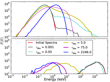
Figure 1.— Radiation spectrum (upper panel) and leptons’ kinetic energy distribution (lower panel) at different simulation stages for a photon-rich plasma ($N_{\gamma}/N_{\rm{lep}}=1000$) with a sudden injection of thermal energy in the lepton population (see Sect. 3.1.1). The legend displays the various optical depths at which if energy was injected, the corresponding color coded spectrum and distribution would be observed.

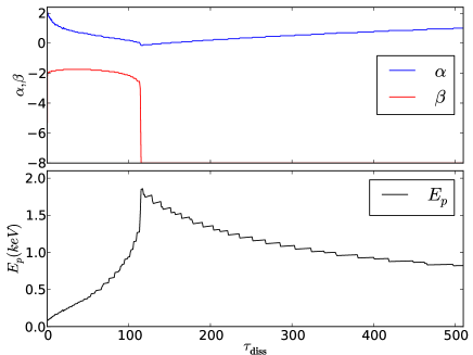
Figure 2.— Evolution of the Band parameters $\alpha$, $\beta$ and, $E_{p}$ of spectra from the simulation shown in Figure 1. The x-axis indicates the optical depth of energy injection.

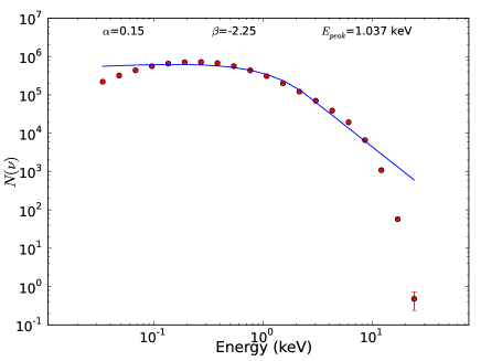
Figure 3.— Fitting of the Band parameters $\alpha$, $\beta$ and $E_{p}$ of spectra from the simulation shown in Figure 1 at $\tau_{diss}=103$.

The results of the simulation are shown in Figure 1, where the evolution of the radiation spectrum and of the spectrum of the kinetic energy of the leptons’ population are displayed. We first note that the final distributions (blue curves in both panels) are all thermal, as expected for a plasma in equilibrium. Looking at the intermediate spectra in more detail, we notice that the immediate reaction of the radiation spectrum is the formation of a high-frequency non-thermal tail, initially appearing as a new component (for spectra at $\tau_{diss}=0.001$) and subsequently forming a continuous tail stemming from the thermal photon population ($\tau_{diss}=5$). At a subsequent stage, the low-frequency part of the radiation spectrum is also modified, with the spectral peak migrating to higher frequencies and causing a flattening of the low-frequency component ($\tau_{diss}=75$). The figure shows that the spectrum takes a very large number of scatterings for equilibrium restoration, especially for frequencies lower than the peak. For energy dissipation at optical depths up to $\sim 100$ a high-frequency non-thermal tail is observed. A non thermal low-frequency tail is instead observed even for a larger optical depth, up to a few thousand.

In order to quantify our synthetic transient spectra and compare them with observations, we fit them to an analytic model. We adopt the widely used Band function (Band et al. 1993) and fit it to the data over a frequency range of three orders of magnitude. Although the GRB spectra are in most cases more complex than a Band function (e.g. Burgess et al. 2014, Guiriec et al. 2011, 2013) this still constitutes a zero-order test that any model should pass. We begin by computing the mean frequency from our data and select neighboring frequencies within 1.5 orders of magnitude around the mean. This data set is binned in frequency and a best-fit Band function is obtained by minimizing the $\chi^{2}$.

Figure 2 shows the evolution of the spectral parameters $\alpha$, $\beta$ and $E_{p}$ for increasing optical depths. We again emphasize that this should not be considered as a time evolution, since the number of scattering is set by the optical depth at which the energy is released in the leptons. A sample fit of the spectrum at $\tau_{diss}=103$ to the Band function is shown in Figure 3. The figure represents a typical case, and shows that the Band model fits well the frequencies around the peak but deviations are observed for the lowest and highest frequencies. We will address this issue further in the discussion. The legend at the top of the figure shows the Band parameters for the fit. An interesting aspect of these simulations is that the low-frequency photon index $\alpha$ and the peak frequency are strongly anti-correlated. This is due to the fact that it is necessary that the peak frequency shifts to higher values for the low-frequency spectrum to change from its thermal equilibrium shape. We also note that the high-energy slope anticipates the low-energy one, the non-thermal features building-up earlier and disappearing faster. We will discuss in more detail these correlations and their implications in Section 4.

3.1.2 Maxwellian leptons at $10^{8}$ K with a power law tail $p=2.2$

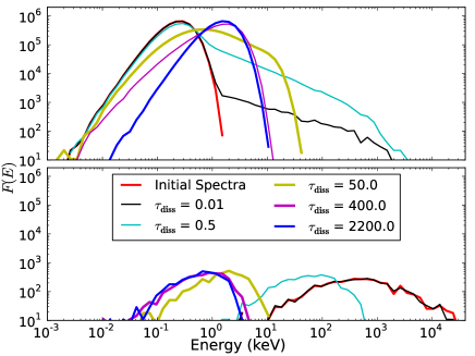
Figure 4.— Color coded photon spectrum (upper panel) and leptons’ kinetic energy distribution (lower panel) at different stages for the photon-rich simulation discussed in Section 3.1.2. The legend displays the various optical depths at which if energy was injected, the corresponding color coded spectrum and distribution would be observed.

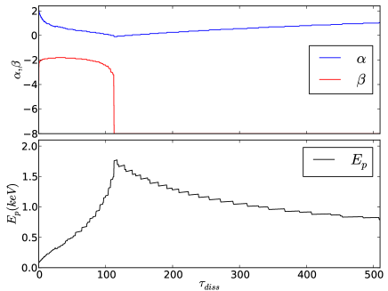
Figure 5.— Evolution of the Band parameters $\alpha$, $\beta$ and $E_{p}$ of spectra from the simulation shown in Figure 4. The x-axis indicates the optical depth of energy injection.

Most models of internal shocks predict the acceleration of non-thermal particles. Comptonization of seed thermal photons by non-thermal leptons has been widely studied in different scenarios and under different assumptions (e.g. Giannios 2006; Pe’er et al. 2005, 2006). In this scenario the shock generates a non-thermal lepton distribution characterized by

$$N(E)dE\propto\gamma^{-p}d\gamma$$ (13)

where $\gamma$ is the lepton Lorentz factor and $p=2.2$. The results of the simulation are shown in Figure 4, where we present the evolving radiation spectrum and distribution of the kinetic energy of the leptons’ population. We notice that the equilibrium photon and lepton distributions (blue curves) are thermal, as expected at equilibrium. We also notice that the spectrum appears non-thermal for a wide range of opacities. Initially a prominent high-energy power-law tail is developed, for a very small opacity (or $\tau_{diss}\sim 0.01$). As the injection opacity increases, the power-law tail is truncated at progressively lower frequencies, the peak frequency shifts to higher values, and a non-thermal tail at low-frequencies develops. The high-frequency tail disappears for $\tau_{diss}\sim 400$, but even larger opacities are required to turn the low-frequency tail back to the scattering-dominated equilibrium spectrum. We fit the Band function to our synthetic spectra and obtain Figure 5, which shows the evolution of the spectral parameters $\alpha$, $\beta$ and $E_{p}$ for increasing injection optical depths. We also notice correlations between the spectral parameters $\alpha$ and the peak frequency, as discussed in Section 3.1.1.

3.1.3 Discrete Multiple Energy Injections

The presence of multiple minor shocks has been emphasized in 2D axisymmetric numerical simulations of jets in collapsars (e.g. Lazzati et al. 2009) and seem to be an even more common feature in 3D simulations (López-Cámara et al. 2013). Hence, to provide a more realistic scenario for the energy injection we explore lepton heating by multiple energy injections mimicking multiple shocks instead of a single more powerful one. The total energy injected into the lepton population is identical to the amount injected in the simulations discussed in Sections 3.1.1 and  3.1.2. However, the energy is divided into 10 equal and discrete partitions with each one being injected and distributed uniformly among the leptons, after every million scatterings.

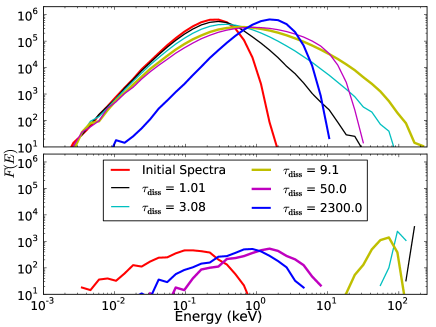
Figure 6.— Photon spectrum (upper panel) and leptons’ kinetic energy distribution (lower panel) at different stages of the simulation discussed in Section 3.1.3. The legend associates the various optical depths of energy injection with the corresponding color coded spectrum and distribution observed.

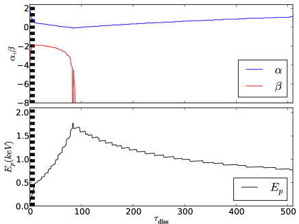
Figure 7.— Evolution of the Band parameters $\alpha$, $\beta$ and $E_{p}$ of spectra from the simulation shown in Figure 6. The x-axis displays the opacity at which energy deposition occurred.

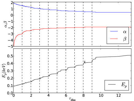
Figure 8.— Magnified version of Figure 7 depicting the response of the Band function parameters $\alpha$, $\beta$ and $E_{p}$ to discrete and multiple energy injections, indicated by the broken black vertical lines. The x-axis displays the opacity at which energy deposition occurred.

The results of the MC simulation are shown in Figure 6, where the evolving radiation spectrum and the spectrum of the kinetic energy of the leptons’ population are displayed. In comparison to Figures 1 and 4, two differences are apparent for small optical depths. First, the high-frequency tail develops much more slowly. Secondly, the slowly developing tail does not extend to the same high energies and in fact, it never approaches the MeV mark. Neither of these differences is surprising, given that a smaller amount of energy is injected at regular intervals. The results of the Band function fitting are reported in Figure 7 and bring to our attention that like previous other simulations, the high-frequency photon index $\beta$ is the first to respond, and also the first to drop just when the $\alpha$ parameter reaches it’s minimum value. Another remarkable aspect of the multiple injection scenario is the immediate reaction of the spectrum to new injections, especially for the high-frequency photon index and the peak frequency (see Figure 8).
What is perhaps mostly interesting, rather than the subtle differences among the three scenarios discussed here, is the fact the Band parameters of Figures 2,  5, and 7 show remarkably similar behavior, even though the injection scenarios are very different. In all three cases, injection at low optical depth only produces a high-frequency power-law tail. Injection at moderate optical depths ($\tau_{diss}\sim 10-100$) produces a high-frequency power-law tail, a shift in the peak frequency, and a non-thermal low-frequency tail. Injection at high to very high optical depths only results in a non-thermal low-frequency tail (see also Section 4 for a discussion).

3.2. Pair Enriched Plasmas

In this section we investigate plasmas enriched by $e^{-}e^{+}$ pairs, by choosing $n_{\gamma}/n_{\rm{lep}}=10$. GRB plasmas can become pair enriched via energy injection through shocks/magnetic dissipation (Rees & Meszaros 2005; Meszaros et al. 2002; Pe’er & Waxman 2004) and if the peak energy of the resulting distribution exceeds 20 keV (Svensson 1982). The generation of pairs is also evident from the photon and lepton distributions crossing the 511 keV mark as shown in the simulations in Sections 3.1.1 and 3.1.2. We assume, as in the previous scenario, that the the pair enriched leptons are impulsively heated by injecting equal amounts of kinetic energy $K/10$ for the first two simulations, albeit with different distribution functions (Maxwellian and Maxwellian plus power law). The third simulation explores the spectral evolution of a pair enriched plasma with an even greater kinetic energy injection. The initial photon count of the plasma $N_{\gamma}$ is $1.01\times 10^{5}$. Being pair-enriched, the total lepton count $N_{e}$ of the plasma is $1.01\times 10^{4}$,

$$N_{e}=N_{e^{-}}+2N_{e^{+}e^{-}}=10^{2}+10^{4}$$ (14)

where $N_{e^{-}}$ are electrons associated with protons and $N_{e^{+}e^{-}}$ denotes the number of pairs in the system.

3.2.1 Maxwellian leptons

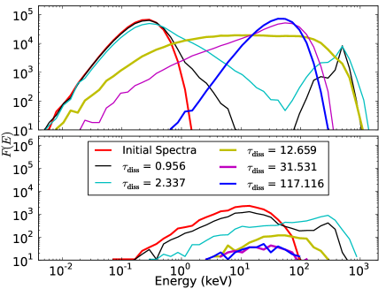
Figure 9.— Photon spectrum (upper panel) and leptons’ kinetic energy distribution (lower panel) at different stages of the pair-enriched simulation discussed in Section 3.2.1. The legend displays the various optical depths at which if energy was injected, the corresponding color coded spectrum and distribution would be observed.

Figure 10.— Evolution of the Band parameters $\alpha$, $\beta$ and $E_{p}$ of spectra from the simulation shown in Figure 9 for increasing values of energy-injection optical depths.

We initiate the simulation with Maxwellian pair-enriched leptons that have been impulsively heated to $10^{8}$ K, thereby taking the population out of equilibrium with the photons. The results of the simulation are displayed in Figure 9 with the upper panel depicting the photon spectra and the lower panel illustrating the kinetic energies of the leptons. Firstly, as observed in the section on photon rich plasmas, the final (blue curve) spectra is consistent with the equilibrium Wien distribution. For $\tau_{diss}\sim 1$ a bump is observed to spike near the annihilation line along with a power law tail (black curve). The lepton distribution also displays a two component distribution (black curve in the lower panel). For $\tau_{diss}\sim 2.3$, the power law tail extends farther to high frequencies and merges with the annihilation bump (cyan curve). On increasing the injection opacity to around $13$, the low frequency spectrum flattens, the peak frequency increases and the annihilation bump merges completely with the initial Wien distribution (or the remnant of the initial spectrum) creating a non-thermal flattened plateau-like feature (yellow curve). The high-frequency power law tail returns to the equilibrium Wien spectrum much earlier ($\tau_{diss}\leq 32$) than the non-thermal low frequency tail, which requires about ($\tau_{diss}\sim 100$) to form the equilibrium spectrum. We interpret this behavior to the inability of the plasma to support a large population of pairs. As a consequence the pairs quickly annihilate and a large amount of $\sim 511$ keV photons are injected in the plasma.
The Band parameters obtained by fitting the Band functions to the simulation spectra are plotted in Figure 10. We note that for moderate optical depths, $\alpha=-0.75$ and $\beta=-1.15$ which corresponds to an extremely non-thermal spectrum. We also observe from the lower panel of Figure 10 that $E_{p}=20-40$ keV. Furthermore, an anti-correlation is observed between the Band parameters $\alpha$ and $\beta$ and between $\alpha$ and $E_{p}$.

3.2.2 Maxwellian leptons at $10^{8}$ K with a power law tail

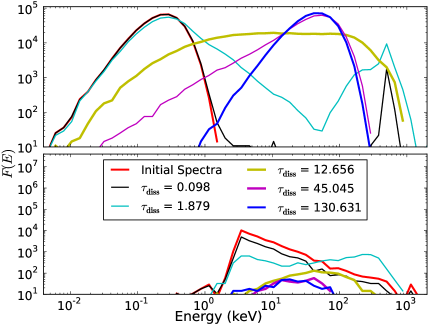
Figure 11.— Photon spectrum (upper panel) and leptons’ kinetic energy distribution (lower panel) at different stages of the simulation discussed in Section 3.2.2. The legend associates the various optical depths of energy injection with the corresponding color coded spectrum and distribution observed.

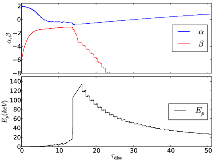
Figure 12.— Evolution of the Band parameters $\alpha$, $\beta$ and $E_{p}$ of spectra from the simulation shown in Figure 11. The x-axis displays the opacity at which energy injection occurred.

This simulation initializes the lower energy lepton population as thermally distributed at $10^{8}$ K and a higher energy population with a power law tail. However, pair enrichment and constraining the injected kinetic energy to $K/10$ lowers the average kinetic energy per lepton in comparison to the photon-rich plasmas. As a result the leptons are generated according to the distribution

$$N(E)dE\propto(\gamma-1)^{-p}d(\gamma-1)$$ (15)

where $\gamma$ is the lepton’s Lorentz factor and $p=2.2$. The red curve in lower panel of Figure 11 displays the initial kinetic energy distribution of the lepton population. Note that the power law tail does not extend to high energies as the tail in Figure 4 does. The figure also shows the evolution of the photon spectra and leptons’ kinetic energy as equilibrium restoration occurs. For the photons, the initial spectra (red curve) and equilibrium spectrum (blue curve) fit the Wien distribution. As is expected, pair annihilation produces a hump in the vicinity of the 511 keV region. Meanwhile, the photons forming the initial Wien spectrum form a power law tail. Similar to the previous scenario, at around $\tau_{diss}\sim 2$ , the power law extends to high frequencies and merges with the growing annihilation hump (cyan curve). We also observe a two component distribution in the lepton panel. By $\tau_{diss}\sim 13$, the two component spectrum transforms into a broad band flat-plateau like spectrum (yellow curve) with the low-frequency spectrum being modified as well. The high frequency spectrum of the magenta curve (for $\tau_{diss}\sim 45$) assumes the exponential cut-off of the Wien spectrum while the low-frequency tail is still prominent. These features make the transient spectra highly non-thermal.
A comparison of Figure 9 with Figure 11 informs us that the spectra of these two scenarios are quite similar. Consequently, a comparison among Figure 10 and Figure 12 also exhibits very similar results - including the anti-correlations between $\alpha$ and peak frequency and between $\alpha$ and $\beta$.

3.2.3 Maxwellian leptons at $10^{8}$ K with a power law tail $p=2.2$

This section explores the system when pair enriched leptons are distributed according the Maxwell-Boltzmann distribution at $10^{8}$ K for lower energies whereas the high energy ones form a power-law tail with index $p=2.2$.

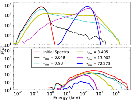
Figure 13.— Photon spectrum (upper panel) and leptons’ kinetic energy distribution (lower panel) at different stages of the pair-enriched simulation discussed in Section 3.2.3. The legend associates the various optical depths of energy injection with the corresponding color coded particle spectrum and distribution.

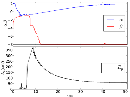
Figure 14.— Evolution of the Band parameters $\alpha$, $\beta$ and $E_{p}$ of spectra from the simulation shown in Figure 13 with increasing energy-injection opacity.

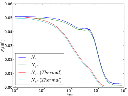
Figure 15.— Evolution of lepton count $N_{e}$ for the simulations in Section 3.2.1 (labeled as $Thermal$) and 3.2.3. Note that the lepton count evolution of the simulations discussed in Sections 3.2.1 and 3.2.2 is indistinguishable. The x-axis displays the opacity at which energy injection occurred.

Similar to the previously discussed cases, the photon spectrum fits the Wien spectrum at equilibrium in Figure 13. A remarkable difference between Figure 13, and between Figures 9 and 11 is that the high frequency power law tail catches up with the pair-annihilation much earlier $(\tau_{diss}<<0.05)$ as depicted by the black curve. Remnants of the hump are visible in the black and cyan curves. Furthermore, for less than 1 scatterings, the low frequency tail becomes softer than the Wien spectrum (cyan curve). Another important non-thermal feature is the broadband nature of the flattened spectrum (the yellow curve extends over four orders of magnitude in frequency). By about $\tau_{diss}\sim 14$, the truncated high frequency tail approaches the exponential cut-off of the Wien spectrum, whereas the soft low frequency tail still persists.
The best-fit Band function obtained by $\chi^{2}$ minimization technique, produces highly non-thermal spectral indices ($\alpha$ and $\beta$) but the peak frequency as shown in Figure 14 is relatively high for GRBs. The lack of smoothness in the $\alpha$ values for moderate optical depths is due to the flatness of the photon spectrum as seen from the yellow curve in Figure 13, which occurs in conjunction with the transient saturation phase in the lepton count (see Figure 15). Figure 15 also displays and compares the lepton count for the simulation in Section 3.2.1 (the curves labeled as $Thermal$, which are indistinguishable from the pair evolution in Section 3.2.2). Although the initial lepton content of the plasmas in the three discussed simulations is identical, the plasma with a greater kinetic energy injection can sustain pairs for larger optical depths leading to a much broader and flatter spectrum. For moderate number of scatterings, we obtain $\alpha=-1$ and $\beta=-0.95$. Again, an anti-correlation is found to exist between the parameters $\alpha$ and $\beta$ and also between $\alpha$ and the peak frequency.

4. Summary and Discussion

We present Monte Carlo simulations of Compton scattering, $e^{-}e^{+}$ pair production, and $e^{-}e^{+}$ pair annihilation in GRB fireballs subject to mild to moderate internal dissipation. We explore cases of photon-rich media – as expected in baryonic fireballs – and of pair-dominated media. The leptonic component in our simulations is initially set out of equilibrium by a sudden injection of energy and the spectrum is followed as continuous collisions among photons and leptons restore equilibrium.

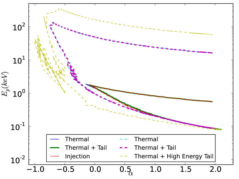
Figure 16.— Plot of Band parameters $E_{p}$ and $\alpha$ for the various simulations discussed. The solid curves represent photon-rich plasmas ($\frac{N_{\gamma}}{N_{lep}}=1000$) whereas the broken curves are indicative of pair-enriched plasmas where ($\frac{N_{\gamma}}{N_{lep}}=10$). Note the similarity among the curves and the exhibited anti-correlation.

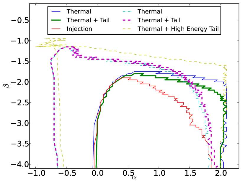
Figure 17.— Plot of Band parameters $\beta$ and $\alpha$ for the various simulations discussed. The solid curves represent photon-rich plasmas ($\frac{N_{\gamma}}{N_{lep}}=1000$) whereas the broken curves are indicative of pair-enriched plasmas where ($\frac{N_{\gamma}}{N_{lep}}=10$). Note the complex behavior of the curves, especially the evolution of $\beta$.

We find that non-thermal spectra arise from transient effects. Such spectra could be advected by the expanding fireball and released before equilibrium is reached if the dissipation takes place at optical depths of up to several hundred. We show that the transient spectra can be reasonably fit by a Band function (Band et al. 1993) within a frequency range of 2-3 orders of magnitude around the peak and could therefore explain GRB observations. As suggested by Lazzati & Begelman (2010), non-thermal features can arise even if both the photon and lepton distributions are initially thermal, provided that they are at different temperatures. As a matter of fact, we find that the spectrum emerging from the fireball after a dissipation event at a certain optical depth does not depend strongly on the way in which the energy was deposited in the leptons. For the photon-rich cases, the first reaction of the photon spectrum to a sudden energy injection into the leptons is the formation of a high-frequency power-law, either because non-thermal leptons are present or through the mechanism described in Lazzati & Begelman (2010). If the injection happens at moderate optical depths, the peak frequency of the photon spectrum also shifts to higher frequencies and a non-thermal low-frequency tail appears. If the energy injection occurs at somewhat large optical depths, the high frequency tail disappears and the spectrum presents a cutoff just above the peak. The low-frequency non-thermal tail is however very resilient and only if the dissipation takes place at very large optical depths, the equilibrium Wien spectrum is attained. The pair-enriched simulations show a more complex behavior at low optical depths due to pair processes, however we still observe the low frequency tail’s resilient behavior. We show that this phenomenology is rather independent on the details of the energy dissipation process and generated lepton distributions: non-thermal leptons, high-temperature thermal leptons, and multiple discrete injection events all produce similar spectra. For the case of the pair-enriched simulations however, we obtain peak frequencies that are somewhat large in the comoving frame (several hundred keV) making this scenario less interesting for explaining observed burst spectra. However their complex behavior and extreme peak energies offer a tantalizing explanation for the rich diversity observed in peak energies of GRBs (Goldstein et al 2012) especially when the peak energies $>$ MeV.

The conclusion we can glean from this study is therefore that comptonization of advected seed photons by sub-photospheric dissipation continues to be a viable model to explain the prompt gamma-ray bursts spectrum. Agreement is particularly strong when the dissipation occurs at moderate optical depth (of the order of tens) so that both a high- and a low-frequency tail are produced. Dissipation at too low optical depth would only produce a high-frequency tail, while dissipation at too large optical depth would only produce a low-frequency tail. In a GRB dissipation is likely to occur at all optical depths (e.g. Lazzati et al. 2009). The dissipation events that occur at moderate optical depth would therefore be those mostly affecting the spectrum and giving it its non-thermal appearance. Bursts characterized by a Band spectrum over more than three orders of magnitude of frequency remain however challenging for this model, and other effects need to be invoked to avoid deviations from the pure power-law behavior at very low and high frequencies. Among these effects, some studied in the literature are sub-photospheric, radiation mediated multiple shocks (Keren & Levinson 2014), line of sight effects (Pe’er & Ryde 2011) and high-latitude emissions (Deng & Zhang 2014).

4.1. Spectral correlations

Besides finding that the overall shape of the partially Comptonized spectra is qualitatively analogous to what observed in GRBs, we find that this model predicts the existence of two correlations that can be used as a test of its validity. We first notice an anti-correlation between the low-energy photon index $\alpha$ and the peak frequency. The correlation is clearly seen in Figure 16, where results from all simulations are shown simultaneously. All simulations start with the same injected photon spectrum, the common point in the lower right of the diagram. The leptons in all three of the photon-rich simulations are energized to identical total kinetic energies $K$ albeit different distribution functions. It is clear that the evolution of all photon-rich simulations is virtually indistinguishable from each other. As more and more scatterings occur, the peak frequency initially grows and the low-frequency slope flattens. At moderate optical depths ($\sim 100$ in all three cases) the peak frequency reaches its maximum, the high frequency tail disappears (shown in the Figure 17) and the low-frequency tail begins to thermalize, dragging the peak frequency to slightly lower values. The correlation has two branches, a steeper one for $\tau<100$ and a flatter one at $\tau>100$. The second branch corresponds, however, to spectra without a high-frequency tail and is therefore not expected to represent observed GRBs. A similar pattern is followed by the pair-enriched cases, with the main difference that larger peak frequencies are attained along with softer values for $\alpha$ and $\beta$. The evolutionary curves for the pair-enriched cases show complexity due to the presence of pairs especially at low opacities - with the simulation in Section 3.2.3 showing a greater amount of variability due to its ability to sustain pairs by temporarily balancing the number of pair production and annihilation events (see Figure 15).
In addition to the $\alpha-\nu_{\rm{pk}}$ anti-correlation, we also find hints of an anti-correlation between $\alpha$ and $\beta$. This correlation is shown in Figure 17 and is much more complex, reflecting the more complex behavior of the high-frequency spectrum with respect to the low-frequency one. In the case of the high-frequency photon-index $\beta$, the way in which the energy is injected in the lepton population matters, each simulation producing a different track on the graph.

Comparing these predictions to GRB spectral data is not straightforward, since the correlations should not be strong in observational data. Adding together data from different bursts, the correlations in the observer frame would be diluted by the different bulk Lorentz factors of bursts and by the diversity of the particle ratio, radiation temperature, and dissipation intensity among busts and pulses in a single burst. Still, some degree of correlation has been discussed in the literature, with contradictory conclusions as to its robustness. The $\alpha-\nu_{\rm{pk}}$ anti-correlation has been discussed in large burst samples (e.g. Amati et al. 2002; Goldstein at al. 2012; Burgess et al. 2014). The $\alpha$-$\beta$ anti-correlation has been observed for some bursts (Zhang et al. 2011), however it is not a common feature among GRBs.

Photospheric dissipation models have found it difficult to reproduce low frequency photon index $\alpha\sim-1$ and have been unable to explain the GeV emissions (Zhang et al 2011). Figure 13 displays the emission spectra in the rest frame of the burst and once Lorentz boosted the photons forming the high frequency tail reach GeV energies. For low/moderate opacities, our simulations have consistently reproduced the low-energy photon index $\alpha<0$ as shown in Figure 16 thus providing a possible resolution for the mentioned issues. Our current model is unable to reproduce $\alpha<-1.1$ for the parameter space explored, however additional effects such can modify and further soften the low frequency spectra. Analogous studies of comptonization effects in GRB outflows have been performed in the past, for example by Giannios (2006) and Pe’er et al. (2006). Our work differs from both of these previous studies in both content and methodology. Giannios (2006) studied with Monte Carlo techniques the formation of the spectrum in magnetized outflows, considering a particular form of dissipation and assuming that the electrons distribution is always thermalized, albeit at an evolving temperature. Pe’er et al. (2006), instead, used a code that solves the kinetic equations for particles and photons, and considered injection of non-thermal particles (as in our Section 3.1.2) as well as continuous injection of energy in a thermal distribution. None of these previous studies consider impulsive injection of energy in thermal leptons, as discussed here or the case of multiple, discrete injection events. In an attempt to keep our results as general as possible we have performed the calculations in a static medium, rather than in an expanding jet. As long as the opacity at which the dissipation occurs is not too large, this should not be a major limitation, and the advantage is that our results are not limited to a particular prescription for the jet radial evolution. In addition, most of the interesting results (the non-thermal spectra) are obtained for small and moderate values of the optical depth (or, analogously, of the number of scatterings that take place before the radiation is released). It should also be noted that the assumption of an impulsive acceleration of the leptons that does not affect the photon spectra is likely not adequate in a highly opaque medium. A final limitation of this study is that only moderate values of the particle ratio can be explored. This is an inevitable limitation when both the lepton and photon distributions are followed in the scattering process with a Monte Carlo technique. If one of the two significantly outnumbers the other, a very large number of photons (or leptons) are required, making the calculation extremely challenging and would require parallelizing the code. While performing such simulations is important and will eventually become possible, we do not anticipate big phenomenological differences with respect to what we consider here. Even with less electrons, we expect the formation of a high-frequency tail (e.g. Lazzati & Begelman 2010), the subsequent shift of the peak frequency accompanied by a flattening of the low-frequency photon index, and complete thermalization only after many scatterings (i.e., only if the dissipation occurs at a very high optical depth).

References

- (1) Amati, L., Frontera, F., Tavani, M., et al. 2002, A&A, 390, 81
- (2) Amati L. 2006, MNRAS, 372, 233
- (3) Asano, K., Inoue, S., & Mészáros P. 2010, ApJ, 725, L121
- (4) Band, D., Matteson, J., Ford, L., et al. 1993, ApJ, 413, 281
- (5) Blumenthal, G.R., & Gould, R.J. 1970, Rev. Mod. Phys, 42, 237
- (6) Beloborodov A. M. 2010, MNRAS, 407, 1033
- (7) Beloborodov A. M. 2013, ApJ, 764, 157
- (8) Bošnjak Ž., Daigne F., & Dubus G. 2009, A&A, 498, 677
- (9) Burgess, J. M., Ryde, F., & Yu, H.-F. 2014, arXiv:1410.7647
- (10) Coppi P.S., & Blandford R.D. 1990, MNRAS, 245, 453
- (11) Crumley P., & Kumar P. 2013, MNRAS, 429, 3238
- (12) Daigne F., Bošnjak Ž., & Dubus G. 2011, A&A, 526, A110
- (13) Deng, W., & Zhang, B. 2014, ApJ, 785, 112
- (14) Fan Y.-Z., Wei D.-M., Zhang F.-W., et al. 2012, ApJ, 755, L6
- (15) Ghirlanda G., Nava L., Ghisellini G., et al. 2012, MNRAS, 420, 483
- (16) Ghisellini G., Celotti A., & Lazzati D. 2000, MNRAS, 313, L1
- (17) Ghisellini G. 2010, AIPC, 1248, 45f
- (18) Giannios D. 2006, A&A, 457, 763
- (19) Giannios D., & Spruit H. C. 2006, A&A, 450, 887
- (20) Goldstein, A., Burgess, J.M., Preece, R.D., et al. 2012, ApJS, 199, 19
- (21) Gould, R.J., & Schreder, G.P. 1967, Phy.Rev., 155, 1404
- (22) Guetta, D., Spada, M., & Waxman, E. 2001, ApJ, 557, 399
- (23) Guiriec, S., Connaughton, V., Briggs, M., et al. 2011, ApJ, 727, 33
- (24) Guiriec, S., Daigne, F., Hascoët, R., et al. 2013, ApJ, 770, 32
- (25) Hascoët R., Daigne F., & Mochkovitch R. 2013, A&A, 551, A124
- (26) Ito,H., Nagataki, S., Ono, M., et al. 2013, ApJ, 777, 62
- (27) Ito H., Nagataki S., Matsumoto J., et al. 2014, arXiv:1405.6284
- (28) Jauch, J.M., & Rohrlich, F. 1980, Theory of Photons and Electrons (2nd Extended ed.; New York: Springer-Verlag.)
- (29) Keren, S., & Levinson, A. 2014, ApJ, 789, 128
- (30) Lazzati D., Morsony B. J., & Begelman M. C. 2009, ApJ, 700, L47
- (31) Lazzati D., & Begelman M. C. 2010, ApJ, 725, 1137
- (32) Lazzati D., Morsony B. J., Margutti R., et al. 2013, ApJ, 765, 103
- (33) Liang E.-W., Yi S.-X., Zhang J., et al. 2010, ApJ, 725, 2209
- (34) Lloyd N. M., & Petrosian V. 2000, ApJ, 543, 722
- (35) Longair, Malcolm, S. 2011, High Energy Astrophysics, (New York: Cambridge)
- (36) López-Cámara D., Morsony B. J., Begelman M. C., et al. 2013, ApJ, 767, 19
- (37) López-Cámara D., Morsony B. J. & Lazzati D. 2014, MNRAS, 442, 2202
- (38) Lundman C., Pe’er A., & Ryde F. 2013, MNRAS, 428, 2430
- (39) Massaro F., & Grindlay J. E. 2011, ApJ, 727, L1
- (40) Mastichiadis A., & Kazanas D. 2009, ApJ, 694, L54
- (41) McKinney J. C. & Uzdensky D. A. 2012, MNRAS, 419, 573
- (42) Medvedev M. V., Pothapragada S. S. & Reynolds S. J. 2009, ApJ, 702, L91
- (43) Mészáros, P., Ramirez-Ruiz, E., Rees, M. J., et al. 2002, ApJ, 578, 812
- (44) Mészáros P., & Rees M. J. 2000, ApJ, 530, 292
- (45) Mizuta A., Nagataki S., & Aoi J. 2011, ApJ, 732, 26
- (46) Nagakura H., Ito H., Kiuchi K., et al. 2011, ApJ, 731, 80
- (47) Pe’er A., Mészáros P., & Rees M. J. 2005, ApJ, 635, 476
- (48) Pe’er A., Mészáros P., & Rees M. J. 2006, ApJ, 642, 995
- (49) Pe’er A., & Ryde, F., 2011, ApJ, 732, 49
- (50) Pe’er, A., & Waxman, E. 2004, ApJ, 613, 448
- (51) Piran T., 1999, PhR, 314, 575
- (52) Preece R. D., Briggs M. S., Mallozzi R. S., et al. 1998, ApJ, 506, L23
- (53) Rees M. J., & Meszaros P. 1994, ApJ, 430, L93
- (54) Rees M. J., & Mészáros P. 2005, ApJ, 628, 847
- (55) Resmi L., & Zhang B. 2012, MNRAS, 426, 1385
- (56) Rybicki, G.B. & Lightman, A.P. 1979, Radiative Processes in Astrophysics, (New York: John Wiley)
- (57) Ryde, F., & Pe’er A. 2009, ApJ, 702, 1211
- (58) Svensson, R. 1982, ApJ, 258, 335
- (59) Zhang, B., & Yan H. 2011, ApJ, 726, 90
- (60) Zhang, B.B., Zhang, B., Liang, E.-W., et al. 2011, ApJ, 730, 141