Generalization of Carey’s Equality and A Theorem on Stationary Population

Abstract.

Carey’s Equality pertaining to stationary models is well known. In this paper, we have stated and proved a fundamental theorem related to the formation of this Equality. This theorem will provide an in-depth understanding of the role of each captive subject, and their corresponding follow-up duration in a stationary population. We have demonstrated a numerical example of a captive cohort and the survival pattern of medfly populations. These results can be adopted to understand age-structure and aging process in stationary and non-stationary population population models. Key words: Captive cohort, life expectancy, symmetric patterns.

(Appeared in Journal of Mathematical Biology) (Springer)

1. Introduction

The motivation to explore the question from which Carey’s Equality ultimately emerged stemmed from the lack of methods for estimating age structure in insect populations in particular, and in a wide range of animal populations generally. Although various methods exist for estimating the age of individual insects, including the use of mechanical damage, chemical analysis and gene expression, many are costly, most require major training and calibration efforts and none are accurate at older ages. Because of these technical constraints, our concept was to explore the possibility of using the distribution of remaining lifespans of captured insects (e.g. fruit flies) to estimate age structure statics and dynamics. The underlying idea was that the death distribution of all standing populations must necessarily be related to the population from which it is derived, ceteris perabus.

James Carey first observed the symmetric survival patterns of a captive cohort and follow-up cohort of medflies (see for example in [2, 1]). Later it was referred to as Carey’s Equality [3] although a formal mathematical statement on a generalized Equality of Carey’s type was missing. The phenomena of Equality of mean length of life lived by a cohort of individuals up to a certain time, and the mean of their remaining length of life in a stationary population, was well established [12, 11]. Proof of Carey’s Equality in [3] is based on the stationary population property explained in [11] although similar phenomena were also found to be useful in understanding the renewal process, see Chapter 5 in [13]. We have formally stated a fundamental theorem to justify Carey’s Equality under a stationary population model, which would allow us to obtain expected lifetimes of a captive cohort of subjects in which each subject is captured at a different age, starting at birth. Further, we have proved our statement under a certain combinatorial and stationary population modeling set-up. These results are extended to two dimensions for estimating age-structure of wild populations and understanding internal structure of aging process, age-structure of wild populations [4]. One also needs to understand the implications of our results for estimating the age structure in stable populations [5].

2. Main Theorem

Theorem 1.

Suppose $\left(X,Y,Z\right)$ is a triplet of column vectors, where $X=\left[x_{1},x_{2},\cdots,x_{k}\right]^{T},$ $Y=\left[y_{1},y_{2},\cdots,y_{k}\right]^{T}$, $Z=\left[z_{1},z_{2},\cdots,z_{k}\right]^{T}$ representing capture ages, follow-up durations, and lengths of lives for $k-$subjects, respectively. Suppose, $F\left(Z\right)$, the distribution function of $Z$ is known and follows a stationary population. Let $G_{1}$ be the graph connecting the co-ordinates of $S_{Y}$, the survival function whose domain is $N(k)=\{1,2,3,...,k\}$ i.e. the set of first $k$ positive integers and $S_{Y}\left(j\right)=y_{j}$ for $j=1,2,...,k.$ Let $G_{2}$ be the graph connecting the co-ordinates of $C_{X},$ the function of capture ages whose domain is $N(k)$ and $C_{X}\left(j\right)=x_{j}$ for all $j=1,2,...,k.$ Suppose $C_{X}^{*}\left(-j\right)=x_{j}$ for all $j=1,2,...,k.$ Let $\mathcal{H}$ be the family of graphs constructed using the co-ordinates of $C_{X}^{*}$ consisting of each of the $k!$ permutations of graphs. Then one of the members of $\mathcal{H}$ $(say,$$H_{g}$) is a vertical mirror image of $G_{1}.$

Proof.

In the hypotheses, the information on capture ages, follow-up durations, and lengths of lives are given as column vectors. For analyzing data collected from life table studies on different organisms (including life expectancy), column vectors are used for representing a convenient data structure, where the matrix of interest has only one column. Capture ages of all subjects in our paper are arranged in a column such that it will be suitable to do addition operations on these ages with a column vector consisting of lives left for corresponding subjects. One also can compute inner product of these two column vectors, but the resultant scalar obtained by such operation is not of interest in the present context. Life table analysis in demography considers column-wise information and each column has a special purpose even though the information obtained from the last column has the key data needed for actuarial modeling, mortality analysis, etc, Using these column vectors of capture ages and follow-up durations from the hypothesis, we have constructed two sets, $I_{1}$ and $I_{2}$.

Let $I_{1}=\left\{\left(i,y_{i}\right):1\leq i\leq k\right\}$ and $I_{2}=\left\{\left(i,x_{i}\right):1\leq i\leq k\right\}.$ $G_{1}$ is constructed using specific ordered pairs of $I_{1}$, explained later in the proof, and $G_{2}$ is constructed by corresponding ordered pairs of $I_{2}.$ There are two criteria, $U_{1}$ and $U_{2},$ that govern the one-to-one correspondence properties of the two functions, $S$ and $C_{X}$.

$$U_{1} = \left\{\mbox{No two subjects are captured who are of the same age and}\right.$$

$$\left.\mbox{there are no two subjects whose follow-up times until death are identical}\right\}$$ .

$$U_{2} = \left\{\mbox{There is more than one subject which has the same capture ages, and}\right.$$

$$\left.\mbox{there is more than one subject which has the same follow-up durations until death}\right\}$$ .

Suppose $f_{1}$ and $f_{2}$ are probability density functions of capture times and follow-up times to death, then by [3], we will have $f_{1}(a)=f_{2}(a)$, which is the probability of an individual who lived ${}^{\prime}a^{\prime}$ years is the same as probability that this individual lives ${}^{\prime}a^{\prime}$ years during the follow-up [3]. For an infinite population in a continuous time set-up for each $x\in C_{X}$ there exists a $y\in S_{Y}$ such that

(2.1) $$\int_{0}^{\infty}x(s)ds+\int_{0}^{\infty}y(s)ds = \int_{0}^{\infty}z(s)ds$$

and

(2.2) $$x_{A} =y_{A} =\frac{1}{2}\int_{0}^{\infty}z(s)ds,$$

where $x_{A}$ and $y_{A}$ are the average capture ages and average follow-up durations until death. Sum of the age at capture of $i^{th}-$ subject (i.e. $x_{i}$) and the follow-up duration (or time left in the current context) of $i^{th}-$subject (i.e. $y_{i}$) is equal to the total length of the life (i.e. $z_{i}$) for the $i^{th}-$subject. See [3, 6] and Chapter 3 in [7] for a description of stationary population models and see page 49 in [8] and see page 52 in [9] for the stationary distributions.

Let’s define $\max\left\{y_{i}\right\}_{i=1}^{k}=y_{t_{1}}$ for some $t_{1}^{th}-$ subject out of $k-$subjects,

$\max\left\{y_{i}:\mbox{for all }i\in N(k)\mbox{ and }i\neq t_{1}\right\}=y_{t_{2}}$ for some $t_{2}^{th}-$subject out of $k-1$ subjects and so on until we arrive at,

$\max\left\{y_{i}:\mbox{for all }i\in N(k)\mbox{ and }i\neq t_{1},t_{2},...,t_{(k-1)}\right\}=y_{t_{k}}$.

$G_{1}$ is constructed by joining the co-ordinates of the set $S$ on the first quadrant, where

(2.3) $$S = \left\{\left(t_{1},y_{t_{1}}\right),\left(t_{2},y_{t_{2}}\right),\cdots,\left(t_{k},y_{t_{k}}\right)\right\}.$$

We call each co-ordinate of $S$ as a cell of $S.$ One can visualize, cells in S are made up of ordered pair of co-ordinates, where abscissa is the subject captured and ordinate is the life left for this subject after capture. Here, the graph, we mean by a curve obtained by joining the cells in $S$. Each cell, except the first and the last cell of S are joined to both sides of its neighboring cells. In case there is more than one subject with a maximum value at one or more stage above, it will lead to two or more identical co-ordinates that are used in $G_{1}.$ When $S$ satisfies $U_{1},$ $G_{1}$ is a graph of decreasing function; when $S$ is satisfies criterion $U_{2},$ $G_{1}$ is a graph of combination of decreasing and non-decreasing functions.

We can construct a sequence of quantities $x_{u_{1}},$$x_{u_{2}},\cdots,$$x_{u_{k}}$ similarly to $S$ to form the set $T$, given below:

(2.4) $$T = \left\{\left(u_{1},x_{u_{1}}\right),\left(u_{2},x_{u_{2}}\right),\cdots,\left(u_{k},x_{u_{k}}\right)\right\}$$

Corresponding to $\left(t_{1},y_{t_{1}}\right)\in S$ there exists a $\left(j,x_{j}\right)\in I_{2}$ which could be $\left(u_{1},x_{u_{1}}\right)$ or some other cell in $T.$ Note that, $C_{X}^{*}=\left\{\left(-j,x_{j}\right):1\leq j\leq k\right\}$. Corresponding to $\left(t_{1},y_{t_{1}}\right)\in S$ if there exists a cell $\left(\left|-i\right|,x_{i}\right)\in C_{X}^{*}$ such that $\left|t_{1}-\left|-i\right|\right|=0$ and $\left|y_{t_{1}}-x_{i}\right|=0$ then we call $\left(t_{1},y_{t_{1}}\right)$ and $\left(\left|-i\right|,x_{i}\right)$ are a pair of equidistant cells from a vertical axis. We can construct a graph $H_{1}$ using cells of $C_{X}^{*}$ in the natural order of integers. In total, we can have $k!$ permutations of orders to construct $H_{1,\cdots,}H_{k!}$. Suppose we denote the first combination of cells as $\left\{\left(-j^{(1)},x_{j}^{(1)}\right):1\leq j\leq k\right\}$ and the second combination of cells as $\left\{\left(-j^{(2)},x_{j}^{(2)}\right):1\leq j\leq k\right\}$ and so on. Negative index here indicates that the subject captured is considered on the negative $x-$axis, which is similar to the left part of the Figure 5.1, if we consider the values 25, 50 75 and 100 for pre-capture segment as -25, -50, -75 and -100 as we visualize them on the negative $x-$axis. Thus by previous arguments, a family of graphs $\mathcal{H}$ is constructed. One of these combinations, for example, the $g^{th}$ combination, is used to construct a graph which we denote with $H_{g},$ which satisfies following Equality:

$$\left|t_{1}-\left|-1\right|^{(g)}\right|=0 \left|y_{t_{1}}-x_{1}^{(g)}\right|=0$$ and

$$\left|t_{2}-\left|-2\right|^{(g)}\right|=0 \left|y_{t_{2}}-x_{2}^{(g)}\right|=0$$ and

$$\vdots \vdots$$

$$\left|t_{k}-\left|-1\right|^{(g)}\right|=0 \left|y_{t_{k}}-x_{k}^{(g)}\right|=0$$ and

here $\left\{\left(\left|-1\right|^{(g)},x_{1}^{(g)}\right),\left(\left|-2\right|^{(g)},x_{2}^{(g)}\right),\cdots,\left(\left|-k\right|^{(g)},x_{k}^{(g)}\right)\right\}$ are $g^{th}$ combination of cells such that $H_{g}$ is a vertical mirror image of $G_{1}.$ Image of $G_{1}$ is visualized as if it is seen from the mirror kept on $y$-axis. Note that, we have generated $k!$ graphs by our construction, and one of such graph, which we called as $H_{g}$ is shown to have vertical mirror image of $G_{1}$. ∎

Our theorem establishes existence of graph depicting mirror images of the pre- and post-capture longevity distributions in Figure 5.1. In general, in the area of population biology where survivorship curves of captive cohort obey Carey’s Equality, there is a need for understanding the pattern within the data structure. The results by [3, 11] explain functional symmetries as an application of renewal theory. We do not depend on any of the classical works on renewal equation and renewal theory proposed by Lotka [14, 15, 16, 17] and by Feller [18] (also see Chapter XI in [19]). Our inspiration is purely from experimental observations demonstrated by James Carey and a statement on stationary populations in the equation (1) in the paper by Vaupel [3]. However, our theory and method of proof uses sequentially arranged data of captive individuals, which was also usually done in renewal theory analysis or proving renewal-type of equations.

Hence our method provide an alternative and independent approach for such kind of sequentially arranged captive subjects. Besides relating the captive ages and corresponding follow-up durations of subjects in a stationary population, the principles of the theorem helped to visualize person-years in a follow-up starting at birth, in a stationary population model in which subjects of each age are captured.

2.1. Life expectancy

First we construct the age structured survival function using $l(s)$, the number of captured subjects at age $s$ and $l(s_{0})$, the number of subjects at the beginning of the follow-up. Suppose $s_{0}$ is the time at the beginning of the follow-up, $s_{i}$ is the time at the $i^{th}$ time point of observation for $i=1,2,\cdots,k$. Suppose each of the $y_{t_{i}}$ for $i=1,2,\cdots,k$ fall exactly in one of the time intervals $\left(s_{i-1},s_{i}\right)$, then the expectancy of life is $\frac{k+1}{2}$. The probability of death over the time period are $q(s_{i})=\frac{1}{k-i}$ with the survival pattern, $l(s_{i})=k-i$ for $i=1,2,\cdots,k-1$ and $l(s_{k})=0$, $q(s_{k})=1.$ Suppose there are $n_{i}$ number of $y_{t_{i}}$ falling within $\left(s_{i-1},s_{i}\right)$ such that $\sum_{i=1}^{k}n_{i}=k$ and $l(s_{i})$ follows the previous construction. If $n_{i}>1$ in one or more of the $\left(s_{i-1},s_{i}\right)$ then there must exist empty cells where the event of death is avoided. Let us define a number $c_{1}$ as follows:

$$c_{1} = \left\{\mbox{Number of cells }(s_{i-1},s_{i})\mbox{ for }\mbox{ }i=1,2,\cdots,k\mbox{ where exactly one of the }\mbox{ }y_{t_{i}}\mbox{ falls }\right\}$$

If $c_{1}=k$, then the life expectancy is $\frac{k+2}{2}$. If $c_{1}\neq k$, then at least one of the $(s_{i-1},s_{i})$ is empty. There could be several combinations of distribution of $y_{t_{1}}$ in $(s_{i-1},s_{i})$ when the event $c_{1}\neq k$ occurs, and we explain in the following remark one possible situation in which deaths are concentrated in the early ages and at late ages. Other combinations can be evaluated using similar constructions.

Remark 1.

Suppose $n_{1}=n_{2}=\cdots=n_{r_{1}}=1$; $n_{r_{1}+1}=n_{r_{1}+2}=\cdots=n_{r_{2}}=0$; and $n_{r_{2}+1}=n_{r_{2}+2}=\cdots=n_{k}=1$ such that $\sum_{i=1}^{k}n_{i}=k$ for some $1<r_{1}<r_{2}<k.$ The probability of death at various ages, $q(s_{i})$, is,

(2.12) $$q(s_{i}) = \left\{\begin{array}[]{cc}\frac{1}{k-i}&\mbox{ for }i=0,1,\cdots,(r_{1}-1)\\ \\ 0&\mbox{ for}\mbox{$$}i=r_{1},(r_{1}+1),\cdots,(r_{2}-1)\\ \\ \frac{1}{k-(r_{1}+i)}&\mbox{ for }i=0,1,\cdots(k-2)\\ \\ 1&\mbox{ for }i=(k-1)\end{array}\right.$$

The life expectancy, $e(s_{0})$, is obtained by the formula below:

$$e(s_{0}) = \frac{1}{2k}\left[\sum_{i=1}^{2r_{1}-1}\left\{2k-i\right\}+\sum_{j=2r_{1}+1}^{2k-1}\left\{2k-j\right\}\right]+\frac{\left(k-r_{1}\right)\left(r_{2}-r_{1}-1\right)}{k}$$

2.2. Person-years and means

Under the above set-up, in this section we derive the mean age of the captive cohort in terms of the mean of the person-units followed. Suppose $a(k,x)$ denotes $k^{th}-$subject ($k>0)$ is captured at age $x$, then $\int_{1}^{\infty}a(k,x)dk$ is number of subjects captured at age $x.$ The mean age at capture for all subjects of the cohort formed of subjects of all ages, $c(0)$, is

(2.14) $$c(0) = \frac{\int_{0}^{\infty}\left[x\int_{1}^{\infty}a(k,x)dk\right]dx}{\int_{0}^{\infty}\int_{1}^{\infty}a(k,x)dkdx}.$$

Let $\int_{0}^{s}b(y)dy$ be the number of deaths out of $\int_{0}^{\infty}\int_{1}^{\infty}a(k,x)dkdx$ during the age $0$ to $s$. The number of subjects surviving at age $s$ is

$$\int_{0}^{\infty}\int_{1}^{\infty}a(k,x)dkdx-\int_{0}^{s}b(y)dy$$

and the number of subjects surviving at age $(n+1)s$ for some positive integer $n$ is

$$\int_{0}^{\infty}\int_{1}^{\infty}a(k,x)dkdx-\sum_{n=0}^{\infty}\int_{ns}^{(n+1)s}b(y)dy.$$

Thus, life expectancy at the formation stage of a captive cohort, say, $E[c(0)]$ can be computed by the formula

(2.15) $$E[c(0)] = \frac{\int_{0}^{\infty}\int_{0}^{\infty}\int_{1}^{\infty}a(k,x)dkdxds-\int_{0}^{\infty}\left(\sum_{n=0}^{\infty}\int_{ns}^{(n+1)s}b(y)dy\right)ds}{\int_{0}^{\infty}\int_{1}^{\infty}a(k,x)dkdx}$$

We state a theorem for the total person-years to be lived by all the subjects in a birth cohort.

Theorem 2.

Suppose subjects of each age of life in a population are captured. Then, using the constructions in $c(0)$ and $E[c(0)]$, the total person-years, say, $T\left(a,c(0),E[c(0)]\right)$, that will be lived by newly born subjects in a stationary population can be expressed as

$$T\left(a,c(0),E[c(0)]\right) = \left(c(0)+E[c(0)]\right)\int_{0}^{\infty}\int_{1}^{\infty}a(k,x)dkdx.$$

Proof.

We have,

(2.16) $$\left(c(0)+E[c(0)]\right)\int_{0}^{\infty}\int_{1}^{\infty}a(k,x)dkdx = \int_{0}^{\infty}\left[x\int_{1}^{\infty}a(k,x)dk\right]dx+$$

$$\int_{0}^{\infty}\int_{0}^{\infty}\int_{1}^{\infty}a(k,x)dkdxds-\int_{0}^{\infty}\left(\sum_{n=0}^{\infty}\int_{ns}^{(n+1)s}b(y)dy\right)ds$$

$$= \int_{0}^{\infty}\left[x\int_{1}^{\infty}a(k,x)dk\right]dx+$$

$$\int_{0}^{\infty}\left[\int_{0}^{\infty}\int_{1}^{\infty}a(k,x)dkdx-\sum_{n=0}^{\infty}\int_{ns}^{(n+1)s}b(y)dy\right]ds$$

The R.H.S. of (2.16) is sum of ages of subjects of all ages in a captive cohort, and total person-years to be lived by the captive cohort, which is $T\left(a,c(0),E[c(0)]\right)$. ∎

3. History and Related Results

An Equality arising out of symmetries of life lived and life left was named as Carey’s Equality by James Vaupel [3], to highlight the discovery of certain symmetries in his biodemographic experiments by James Carey (see, for example, [2, 1]). Vaupel [3] and Goldstein [11] have proved equality on such symmetries as a direct application of renewal theory. Our main theorem in this article is not inspired by renewal theory, but we conceptualized our approach directly from experimental results shown by James Carey and then used equation (1) from Vaupel [3] in our hypothesis. Renewal theory has long history even before the seminal works on population dynamics by Alfred Lotka (see, for example, [14, 15, 16]), who has used an integral equation of type (3.1) to link number of births at time $t>0$ with number of births a women has at time $t=0.$

(3.1) $$B(t)=\int_{0}^{t}G(t,a)da+H(t)$$

where $B(t)$ is total number of births at time $t$, $G(t,a)$ is number of births from a women who is at age $a$ and alive at time $t$ and $H(t)$ is number of births from a women who is alive at $t=0.$ Usually, we compute $B(t)$ from $a=\alpha$ to $a=\beta$, where $\alpha$ is lower reproductive age and $\beta$ is upper reproductive age. $G(t,a)$ can be written as,

(3.2) $$G(t,a)=B(t-a)s(a)$$

where $B(t-a)$ is total number of births at time $(t-a)$ and $s(a)$ is chance of surviving to exact age $a.$ 3.1 is also referred as renewal equation. Combining 3.1 and 3.2, we can write $B(t)$ within reproductive ages as,

(3.3) $$B(t)=\int_{\alpha}^{\beta}B(t-a)s(a)da$$

William Feller [19] provided foundations of renewal theory in his book (see Chapters VI and XI) as did authors of other books which were written exclusively on renewal theory (see for example, [13]) or contained chapters devoted to basic renewal theory (for example, see Chapter 6 in [9] and Chapter 12 in [20]). Several applications of convolutions of independent random variables which we see in renewal theory can also be found in understanding disease progression between one stage to another stage, epidemic prediction and so forth (for example, see [21] and [22]).

4. Example and visualization

We provide here a practical application based on the medfly population with a visual depiction of Carey’s Equality (Figure 5.1). Note the symmetry of the pre- and post-capture segments of the lifespans of individuals in the population that underlies the equivalency of life-days which, in turn, underlies the equivalency noted by [3], "If an individual is chosen at random from a stationary population…then the probability the individual is one who has lived a years equals the probability the individuals is one who has that number of years left to live.”

Carey’s Equality is important because it both builds on and complements the properties of one of the most important models in demography: the stationary population model. Stationary population model is fundamental to formal demography because it is a special case of the stable population model, and provides explicit expressions that connect the major demographic parameters to one another, including life expectancy, birth rates, death rates and age structure, see Chapter 3 in [7]. A graphical depiction of Carey’s Equality, shown in Figure 5.2, shows the interconnectedness of these parameters. Note that the shape of the stationary population 5.2(a) as well as both its age and death distributions 5.2(b) are identical, and that the proportion of each age class in the captive population 5.2(c) is identical to the proportions within the whole population (i.e. due to the symmetrical distributions of pre- and post-capture lifespans in 5.2(b)).

5. Discussion

The approach we used in this paper to demonstrate the mathematical identity underlying Carey’s Equality is fundamentally different than that used by previous authors. Originally James Carey created a simple life table model (Table 1 in [2]) to demonstrate the equality of age structure and post-capture deaths in a stationary population, the identity of which was then formalized by statisticians Hans Müller and Jane-Ling Wang [2]. Vaupel [3] and Goldstein [11] followed by using mathematical first principles to derive the equality.

Our approach differs from the one we just outlined. Instead of first formulating and then deriving the equality, we justified the constancy of post-capture patterns of death in stationary medfly populations in the following two steps. The first was to conjecture that in stationary populations the ordered pre- and post-capture life course segments of individuals will be symmetrical (Theorem 1) and that total person-years in a captive cohort can be formulated (Theorem 2). The second was to prove these relationships using a series of mathematical assumptions (i.e. the respective proofs).

Our approach contributes to the demographic literature in general and specifically to an understanding of Carey’s Equality in several ways. First, our theorems provide an independent method for formulating a mathematical relationship in formal demography. Indeed we are unaware of any other models in formal demography that have involved proofs from mathematical conjectures (theorems). Second, our proofs allow us to state unequivocally that the Carey Equality will be true in all stationary populations. Although this is a logical outcome from all of the earlier approaches, our approach makes this result both explicit and conclusive. Third, our proofs required that we draw on set theory, an area of mathematics involving logic that is not commonly used in demography. As a consequence of the problem framed in fundamental mathematics, Carey’s Equality is better situated both to draw from and be extended into other areas of basic mathematical theory. Fourth, using the ideas of the main theorem, we are positioned to obtain further results related to Carey’s Equality such as for higher dimensions and probabilistic and deterministic results for multiple captive cohorts.

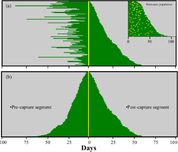
Figure 5.1. Schematics of a randomly sampled hypothetical stationary Mediterranean fruit fly population (adapted from [10]). Horizontal lines depict the life course of individual flies from birth (eclosion) to death. (a) Example of the life courses of captive individuals divided into pre- and post-capture segments and ordered from shortest-to-longest (top-to-bottom) post-capture lifespans. Inset shows the stationary medfly population in which the yellow tick marks depict the ages at which individual medflies are sampled. (b) Same as (a) except with the pre- and post-capture segments of individuals decoupled and both ordered according to length from top-to-bottom to show the symmetry (mirror image) of the distributions.

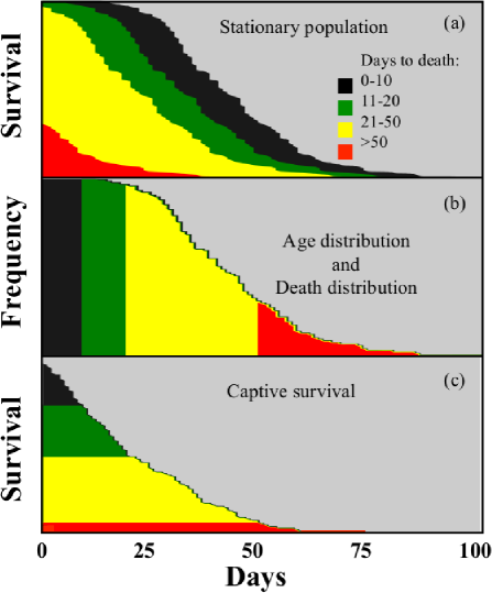
Figure 5.2. Structural interconnectedness of an hypothetical stationary Mediterranean fruit fly population showing: (a) days to death by age groups; (b) age and death distributions; and (c) captive survival.

6. Conclusions

Our paper offers new sets of tools, techniques and theoretical framework in terms of visualization of the demographic data involving capture ages and development of new theoretical ideas for analyzing data obtained by captive cohorts. Such approaches will have applications in other demographic situations, for example, understanding aging patterns in a captive cohort data when information on lives left is right truncated, projecting various scenarios of demographic transition, etc,

The main result of our paper will be useful in understanding the relationship between average lengths of lives of captured, follow-up, and total lengths of the lives in a stationary population. Our method of re-structuring the follow-up durations of captive cohort can be adopted also for non-stationary populations, which can be used for understanding the internal structures of the population with respect to the age at capture. This will enable us to look deeper into the aging process of stationary and non-stationary populations. For each captive cohort of subjects there exists an associated, exact configuration of a combination of coordinates of the survival graphs, and this association is dynamic. The right combination of coordinates is dependent on the formation of the captive cohort. The idea of a proof through formation of symmetric graphs, combined with captive age distribution is novel. We have demonstrated the utility of such thinking in understanding symmetric patterns formed of a captive cohort and associated follow-up lengths. This strategy was also helpful for us in deriving formulae for expectation of life in a stationary population, discretely, and also using multiple integrals. The theory explained here can be adopted to both human and non-human populations.

7. Acknowledgements

We thank the organizers of the Keyfitz Centennial Symposium on Mathematical Demography sponsored by the Mathematical Biosciences Institute, Ohio State University, June 2013. Research by JRC supported by NIA/NIH grants P01 AG022500-01 and P01 AG08761-10.

References

- [1] Carey JR, Papadopoulos N, Müller H-G, Katsoyannos B, Kouloussis N, Wang J-L, Wachter K, Yu W, Liedo P (2008). Age structure changes and extraordinary life span in wild medfly populations. Aging Cell 7, 426-437.
- [2] Müller HG, Wang J-L, Carey JR, Caswell-Chen EP, Chen C, Papadopoulos N, Yao F (2004) Demographic window to aging in the wild: Constructing life tables and estimating survival functions from marked individuals of unknown age. Aging Cell 3, 125-131.
- [3] Vaupel, J. W. (2009). Life lived and left: Carey’s Equality, Demographic Research, vol. 20 (2009), pp. 7-10.
- [4] Arni S.R. Srinivasa Rao and James R. Carey (2014). Behavior of Carey’s Equality in Two-Dimensions: Age and Proportion of Population (Manuscript in-preparation)
- [5] Arni S.R. Srinivasa Rao (2014). Population Stability and Momentum, Notices of the American Mathematical Society. 61, 9, 1165-1168.
- [6] Ryder N.B. (1975). Notes on Stationary Populations, Population Index, 41, 1, 3-28.
- [7] Preston SH, Heuveline P, Guillot M (2001). Demography: Measuring and Modeling Population Processes. Malden, Blackwell Publishers.
- [8] Goswami, A and Rao, B.V. (2006). A course in Applied Stochastic Processes, Hindustan Book Agency (India), New Delhi.
- [9] Lawler G.F. (2006). Introduction to StochasticProcess (2/e), Chapman & Hall/CRC.
- [10] Carey, J. R., Müller, H.-G., Wang, J.-L., Papadopoulos, N. T., Diamantidis, A. & Kouloussis, N. A. (2012) Graphical and demographic synopsis of the captive cohort method for estimating population age structure in the wild. Experimental Gerontology, 47, 787-791.
- [11] Goldstein JR. 2009 Life lived equals life left in stationary populations. Demographic Research 20, 3-6.
- [12] Kim, Y. J. and Aron, J. L. (1989). On the equality of average age and average expectation of remaining life in a stationary population. SIAM Review 31(1): 110–113. doi: 10.1137/1031005.
- [13] Cox, D. R. (1962). Renewal Theory. London: Methuen and Co.
- [14] Lotka, A.J. (1907). Relation between birth rates and death rates. Science N.S , 26:21—22.
- [15] Lotka, A.J. (1939a). A contribution to the theory of self-renewing aggregates with special reference to industrial replacement, Annals of Mathematical Statistics, 10:1-25.
- [16] Lotka, A.J. (1939b). On an integral equation in population analysis. Annals of Mathematical Statistics, 10:144–161.
- [17] Lotka. A.J. (1956). Elements of Mathematical Biology . New York, Inc.,: Dover Publications.
- [18] Feller, W (1941). On the Integral Equation of Renewal Theory, The Annals of Mathematical Statistics, 12 (3): 243-267.
- [19] Feller, W (1971). An Introduction to the Probability Theory and its Applications, Volume II, John Wiley & Sons, 2nd Edition.
- [20] Karlin, S (1969). A first course in Stochastic Process, Academic Press, Inc,
- [21] Brookmeyer, R., Gail, M.H (1988). A method for obtaining short-term projections and lower bounds on the size of the AIDS epidemic J. Am. Stat. Assoc. 83 (402): 301-308.
- [22] Arni S.R. Srinivasa Rao (2015). Incubation Periods Under Various Anti-Retroviral Therapies in Homogeneous Mixing and Age-Structured Dynamical Models: A Theoretical Approach. To appear in Rocky Mountain Journal of Mathematics. (To Appear in 2015). http://projecteuclid.org/DPubS?verb=Display&version=1.0&service=UI&handle=euclid.rmjm/1379596735 &page=record