Short Title: Chicken Walks

Abstract.

Understanding animal movements and modelling the routes they travel can be essential in studies of pathogen transmission dynamics. Pathogen biology is also of crucial importance, defining the manner in which infectious agents are transmitted. In this article we investigate animal movement with relevance to pathogen transmission by physical rather than airborne contact, using the domestic chicken and its protozoan parasite Eimeria as an example. We have obtained a configuration for the maximum possible distance that a chicken can walk through straight and non-overlapping paths (defined in this paper) on square grid graphs. We have obtained preliminary results for such walks which can be practically adopted and tested as a foundation to improve understanding of non-airborne pathogen transmission. Linking individual non-overlapping walks within a grid-delineated area can be used to support modeling of the frequently repetitive, overlapping walks characteristic of the domestic chicken, providing a framework to model faecal deposition and subsequent parasite dissemination by faecal/host contact.We also pose an open problem on multiple walks on finite grid graphs. These results grew from biological insights and have potential applications. Keywords: Spread of bird diseases, Eimeria, Maximum walks, longest paths, NP-Complete. MSC: 92A17, 68Q17

Understanding Chicken Walks on $n\times n$ Grid: Hamiltonian Paths, Discrete Dynamics and Rectifiable Paths

Appeared in Mathematical Methods in the Applied Sciences (Wiley-Blackwell) DOI: 10.1002/mma.3301

*Corresponding author.

1. Straight Walk and Non-overlapping Walk

Parasitic pathogens with direct single-host life cycles rarely rely on aerial transmission for dissemination, more commonly featuring direct (i.e. physical contact) or indirect (environmental, food- or water-borne) routes [1]. Examples include protozoans such as Cryptosporidium and Eimeria, helminths such as Ostertagia ostertagi and arthropods such as Sarcoptes scabei. Understanding the transmission of such pathogens requires an awareness of host movement as the initial source of pathogen spread, informed by subsequent environmental factors such as food movement, flow of water and other fomites. Recognition of the relevance of poultry to food security has elevated the importance of their pathogens, with parasites such as Eimeria of key significance [2]. Eimeria can cause the disease coccidiosis, a severe enteritis characterised by high morbidity and, sometimes, mortality. The global cost of losses attributed to Eimeria and their control has been estimated to exceed $3 billion per annum, complicated further by welfare implications [3]. Most Eimeria are absolutely host-specific and exhibit a strict faecal-oral lifecycle including an environmental stage, called the oocyst, which must undergo a process termed sporulation over twelve to thirty hours external to the host in order to become infective. Thus, the physical behaviour of chickens including the amount of time spent moving, the distance moved, the pattern of movement and the frequency and location of defaecation whilst moving are of critical importance to understanding Eimeria transmission. Transmission rates have previously been calculated for Eimeria acervulina [4]. Overlaying these data onto models of chicken movement will support prediction of Eimeria transmission through a flock, facilitating scrutiny of the impact of management system and the opportunity for co-infection by genetically diverse parasite strains [5, 6, 7]. The frequency of co-infection with genetically diverse strains will determine the rate at which cross fertilization may occur, influencing the occurrence of novel genotypes with relevance to evasion from drug- and vaccine-mediated parasite killing [8]. Inspired by the importance of chicken movement in Eimeria transmission, this work grew into an exercise to model chicken movement while studying the length of distance chickens walk per unit time in a pen, their parasite disseminating characteristics and the rate at which infection spreads between birds. In order to understand the complexity of chicken movement we have begun by assuming a square pen which can be subdivided into a cellular graph. The walks considered in this manuscript are of maximum length. By joining several such walks together in the future we will begin to recreate multiple chicken paths as an entrée to modeling chicken movements in more complex environments.

Let us consider an area, $S$, of dimension $n\times n$ ($n>1)$ which is divided into $n\times n-$small squares (or cells). Let $\left(i,j\right)$ be the cell which is located at $i^{th}$ row and $j^{th}$ column of these $n$ cells. Suppose we leave a chicken in one of the cells of $S$ and suppose we are interested in observing the walking behaviour of chicken through the following two rules, i) Walking from one corner point to a neighboring corner point and ii) Walking only through each cell (excluding on the cell boundaries). The $(i,j)^{th}$ cell is denoted by $S_{ij}\left[A_{i},B_{j},C_{j},D_{i}\right]$, where $A_{i}$, $B_{j}$, $C_{j}$ and $D_{i}$ are four vertices of this cell which are located at the upper left corner, upper right corner, lower right corner and lower left corner, respectively. A chicken sitting inside the cell $(i,j)$ (not on the vertices) is denoted by $K(i,j)$ and a chicken sitting on the vertices $A_{i}$, $B_{j}$, $C_{j}$ and $D_{i}$ of $S_{ij}$ is denoted by $K(A_{i})$, $K(B_{j})$, $K(C_{j})$ and $K(D_{i})$ of $S_{ij}$, respectively. A straight walk by $K(i,j)$ is defined here as a walk initiated by $K(i,j)$ for all $i=1,2,\cdots,n$ and $j=1,2,\cdots,n$ by moving to neighboring cell through adjacent sides only and a straight walk by $K(A_{i})$ or $K(B_{j})$ or $K(C_{j})$ or $K(D_{i})$ of $S_{ij}$, respectively, for all $i=1,2,\cdots,n$ and $j=1,2,\cdots,n$ is defined here as a walk from one cell to another cell that shares an edge with the current cell. For example, $K(1,3)$ means that the chicken is in the cell which is at first row and third column and $K(A_{2})$ of $S_{23}$ means chicken is at the vertex $A_{2}$ of cell $S_{23}$ (which is located at second row and third column) which has four vertices $\left[A_{2},B_{3},C_{3},D_{2}\right]$.

We can visualize the area $S$ either with even number of cells $\left(2n\times 2n\right)$ or with odd number of cells $\left((2n+1)\times(2n+1)\right)$ and is placed on a grid graph, $G$, which is a subset of an infinite graph, $G^{\infty}$ [9]. See [9, 10, 11, 12, 13] for foundations on grid graphs and [14, 15, 16, 17, 18, 19] for infinite graphs. If an area $S$ has $\left(2n\times 2n\right)$ cells then it will have $\left((2n+1)\times(2n+1)\right)$ vertices. This gives us some flexibility to construct walks connecting some finite number of cells and relate such walks to the walks through vertices. Using the same flexibility, we define a cell as even if both $i$ and $j$ are even or $i+j$ $\cong$ $0$(mod2). Hence, a maximum possible walk between two cells $(i,j)$ and $(i^{*},j^{*})$ can be considered as an Hamiltonian Path between these two cells. The problem of determining if a given graph G has a Hamiltonian path is NP-Complete [9]. We have described Hamiltonian and related paths through cells in a grid in section 2. The maximum paths between cells that we considered as described above and further discussed in section 3 and 4 are simpler situations than NP-complete problems. Our results indicate maximum possible walks can be configured based on the position of the cells connecting walks in an even dimensional area and an odd dimensional area. Primarily we differ in our approach because we tried all our attempts by connecting maximum possible walks between two cells. However, one can attempt to relate particular cases of our types of walks with Hamiltonian path configurations.

2. Related Works

Our results were not inspired by previous work on Hamiltonian Paths or NP-Complete problems. We obtained the solutions of maximum possible walks from fundamental principles while trying to model chicken walks to understand transmission rates and cross fertilization of certain parasites with strict fecal / oral life cycles among chickens. We have thought of distributing the locations of defecations per unit of time and hence we tried to link two Hamiltonian paths at these locations. Moreover, Hamiltonian Path problems are related to the paths connected between two vertices. See [20, 21] for basic introduction to the Hamiltonian paths. Let $G$ be a finite and simple graph with at least $3$ vertices. Then, by Ore’s Theorem [22], $G$ is Hamiltonian, if for every pair of non-adjacent vertices (say, $a$ and $b$), the sum of the degrees of $a$ and $b$ is at least $3.$ Ore’s Theorem is based on the arguments of the work by Newman [23] who proved that “Any graph with $2n$ vertices each of order not less than n must contain a $2n-gon$”. A graph $G$ is called Ore-type $(k)$ if it satisfies $d(a)+d(b)\geq\left|G\right|+k$, where $d(a)$ and $d(b)$ are degrees of $a$ and $b,$ respectively. $G$ is $k-path$ Hamiltonian if $G$ is a graph on $p$ vertices and $d(a)+d(b)\geq p+k$ for every pair $\left\{a,b\right\}$ [24]. In general, when $G$ has $p$ vertices, then $G$ is $k-path$ Hamiltonian if $G$ has at least $\frac{1}{2}(p-1)(p-2)+k+2$ edges [24]. This condition is sufficient for a graph to be $k-path$ Hamiltonian. For works on the longest paths in undirected graphs (random) refer to [25, 26, 27]. Algorithms for approximating the longest paths in grid graphs and meshes can be seen here [28, 29, 30, 31, 32]. There are methods which are based on the longest paths in random graphs (for example, see [25]) and search for the trees formed by probability processes [33, 34]. Using the Turing machine-based models, computational complexity of $k-path$ problems were studied (see [35]) and for the importance of finding a path in a plane, see [36].

3. Maximum Possible Walk

In this section we study the properties of obtaining maximum possible walks under the hypotheses of straight and non-overlapping walks.

Theorem 3.1.

(A) Suppose a straight walk is initiated by $K(i,j)$ in $S$ (the maximum distance covered by $K(i,j)$ without stepping onto the same cell cannot exceed $n^{2}-1$), then there exists configurations when the walk is initiated through any neighboring side of the $K(i,j)$.

(B) Suppose a straight walk is initiated by $K(A_{i})$ or $K(B_{j})$ or $K(C_{j})$ or $K(D_{i})$ of $S_{ij}$ in $S$ (the maximum distance covered by each of these walks cannot exceed $(n+1)^{2}-1$), then there exists configurations when the walk is initiated through any neighboring vertex.

Proof.

That maximum distance travelled is $n^{2}-1$ is easy to verify, so we will concentrate here on configurations. (A) We introduce notations for the directions for movement of a chicken between cells either row wise or column wise. A chicken moved from $(i,j)$ to $(i-1,j)$ is denoted by the direction ${}_{(i-1)j}d_{ij}$, similarly a move from $(i,j)$ to $(i,j+1)$ is denoted by the direction ${}_{i(j+1)}d_{ij}$, move from $(i,j)$ to $(i+1,j)$ is denoted by the direction ${}_{(i+1)j}d_{ij}$, move from $(i,j)$ to $(i,j-1)$ is denoted by the direction ${}_{i(j-1)}d_{ij}$.

We prove the theorem in two situations, (I) when $S$ has dimension $2n\times 2n$ and (II) when $S$ has dimension $(2n+1)\times(2n+1)$

(I) $S$ has dimension $2n\times 2n$. Consider a chicken in an arbitrary cell, $(i^{\prime},j^{\prime})$ i.e. $K(i^{\prime},j^{\prime})$. Suppose $(2n-i^{\prime})$ is an odd number, $(2n-j^{\prime})$ is an even number. This means there are an odd number of columns to the right of $K(i^{\prime},j^{\prime})$, an even number of columns to the left of $K(i^{\prime},j^{\prime})$ and an odd number of rows above $K(i^{\prime},j^{\prime})$, an even number of rows below $K(i^{\prime},j^{\prime})$. We prove the statement for each of the four directions.

(a) Starting direction from $K(i^{\prime},j^{\prime})$ is ${}_{(i^{\prime}-1)j^{\prime}}d_{i^{\prime}j^{\prime}}$. Follow the configuration given in the steps shown below:

($a_{1}$) take $(i^{\prime}-1)$ steps in the direction ${}_{(i^{\prime}-1)j^{\prime}}d_{i^{\prime}j^{\prime}}$ to reach the first row, ($a_{2}$) take $(2n-i^{\prime})$ steps in the direction ${}_{1(2n-i^{\prime}+1)}d_{1(2n-i^{\prime})}$ to reach the last column, ($a_{3}$) take $(2n-1)$ steps in the direction ${}_{2(2n)}d_{1(2n)}$ to reach the last row, ($a_{4}$) take one step in the direction ${}_{(2n)(2n-1)}d_{(2n)(2n)}$, ($a_{5}$) take $(2n-2)$ steps in the direction ${}_{(2n-1)(2n-1)}d_{(2n)(2n-1)}$, ($a_{6}$) take one step in the direction ${}_{2(2n-2)}d_{2(2n-1)}$, ($a_{7}$) take $(2n-2)$ steps in the direction ${}_{(2n)(2n-2)}d_{2(2n-2)}$ to reach last row, ($a_{8}$) repeat the steps similar to the steps ($a_{4}$) to ($a_{6}$) to reach the last row and $(2n-j^{\prime}+1)$ column where the given chicken is currently located, i.e. $K\left(2n,(2n-j^{\prime}+1)\right)$, ($a_{9}$) take $(2n-j^{\prime})$ steps in the direction ${}_{(2n)(2n-j^{\prime})}d_{(2n)(2n-j^{\prime}+1)}$ to reach the first column, ($a_{10}$) take $(2n-1)$ steps in the direction ${}_{(2n-1)1}d_{(2n)1}$ to reach the first row, ($a_{11}$) take one step in the direction ${}_{12}d_{11}$, ($a_{12}$) take $(2n-2)$ steps in the direction ${}_{22}d_{12}$, ($a_{13}$) take one step in the direction ${}_{(2n-1)3}d_{(2n-1)2}$, ($a_{14}$) take $(2n-2)$ steps in the direction ${}_{(2n-2)3}d_{(2n-1)3}$ to reach first row, ($a_{15}$) take one step in the direction ${}_{14}d_{13}$, ($a_{16}$) take $(2n-1)$ steps in the direction ${}_{24}d_{14}$, ($a_{17}$) repeat the steps similar to the steps ($a_{8}$) to ($a_{16}$) such that the chicken is located in the $(2n-1)$ row and $(2n-j^{\prime}-1)$ column i.e. $K\left((2n-1),(2n-j^{\prime}-1)\right)$, ($a_{18}$) take one step in the direction ${}_{(2n-1)(2n-j^{\prime})}d_{(2n-1)(2n-j^{\prime}-1)}$, ($a_{19}$) take $(i^{\prime}-2)$ steps in the direction ${}_{(2n-2)(2n-j^{\prime})}d_{(2n-1)(2n-j^{\prime})}$ to reach the cell $\left((2n-i^{\prime}+1\right),(2n-j^{\prime})$ such that we will have $K\left((2n-i^{\prime}+1\right),(2n-j^{\prime})$. This way the chicken takes $4n^{2}-1$ steps, and we achieved maximum distance configuration.

(b) Starting direction from $K(i^{\prime},j^{\prime})$ is ${}_{(i^{\prime})(j^{\prime}+1)}d_{i^{\prime}j^{\prime}}$. Maximum distance configuration is given in the steps shown below:

($b_{1}$) take $(2n-j^{\prime})$ steps in the direction ${}_{(i^{\prime})(j^{\prime}+1)}d_{i^{\prime}j^{\prime}}$ to reach the last column, ($b_{2}$) take $(2n-i^{\prime})$ steps in the direction ${}_{(2n-i^{\prime}+1)(2n)}d_{(2n-i^{\prime})(2n)}$ to reach the last row, ($b_{3}$) take $(2n-1)$ steps in the direction ${}_{(2n)(2n-1)}d_{(2n)(2n)}$ to reach the first column, ($b_{4}$) take one step in the direction ${}_{(2n-1)1}d_{(2n)1}$, ($b_{5}$) take $(2n-2)$ steps in the direction ${}_{(2n-1)2}d_{(2n-1)1}$, ($b_{6}$) take one step in the direction ${}_{(2n-2)(2n-1)}d_{(2n-1)(2n-1)}$, ($b_{7}$) take $(2n-2)$ steps in the direction ${}_{(2n-2)(2n-2)}d_{(2n-2)(2n-1)}$ to reach the first column, ($b_{8}$) take one step in the direction ${}_{(2n-3)1}d_{(2n-2)1}$, ($b_{9}$) take $(2n-2)$ steps in the direction ${}_{(2n-3)2}d_{(2n-3)1}$, ($b_{10}$) repeat the steps similar to the steps ($b_{6}$) to ($b_{9}$) such that the chicken is located in the cell $\left((2n-i^{\prime}+3),(2n-1)\right)$, i.e. $K\left((2n-i^{\prime}+3),(2n-1)\right)$, ($b_{11}$) take two steps in the direction ${}_{(2n-i^{\prime}+1)(2n-1)}d_{(2n-i^{\prime}+3)(2n-1)}$, ($b_{12}$) take one step in the direction ${}_{(2n-i^{\prime}+1)(2n-2)}d_{(2n-i^{\prime}+1)(2n-1)}$, ($b_{13}$) take one step in the direction ${}_{(2n-i^{\prime}+2)(2n-2)}d_{(2n-i^{\prime}+1)(2n-2)}$, ($b_{14}$) take one step in the direction ${}_{(2n-i^{\prime}+2)(2n-3)}d_{(2n-i^{\prime}+2)(2n-2)}$,

($b_{15}$) take one step in the direction ${}_{(2n-i^{\prime}+1)(2n-3)}d_{(2n-i^{\prime}+2)(2n-3)}$, ($b_{16}$) repeat the steps similar to the steps ($b_{7}$) to ($b_{15}$) to reach the cell $\left((2n-i^{\prime}+1),1\right)$, ($b_{17}$) continue for $i^{\prime}$ steps in the same direction to reach the cell $(1,1)$, ($b_{18}$) take $(2n-1)$ steps in the direction ${}_{12}d_{11}$ to reach the last column, ($b_{19}$) take one step in the direction ${}_{2(2n)}d_{1(2n)}$, ($b_{20}$) take $(2n-2)$ steps in the direction ${}_{22}d_{2(2n)}$, ($b_{21}$) take one step in the direction ${}_{32}d_{22}$, ($b_{22}$) take $(2n-2)$ steps in the direction ${}_{33}d_{32}$ to reach the last column, ($b_{23}$) repeat the steps similar to the steps ($b_{19}$) to ($b_{22}$) such that the chicken is located in the cell $\left((i^{\prime}-3),2n\right)$, ($b_{24}$) take two steps in the direction ${}_{(i^{\prime}-2)(2n)}d_{(i^{\prime}-3)(2n)}$, ($b_{25}$) take one step in the direction ${}_{(i^{\prime}-1)(2n-1)}d_{(i^{\prime}-1)(2n)}$, ($b_{26}$) take one step in the direction ${}_{(i^{\prime}-2)(2n-1)}d_{(i^{\prime}-1)(2n-1)}$, ($b_{27}$) take one step in the direction ${}_{(i^{\prime}-2)(2n-2)}d_{(i^{\prime}-2)(2n-1)}$, ($b_{28}$) take one step in the direction ${}_{(i^{\prime}-1)(2n-2)}d_{(i^{\prime}-2)(2n-2)}$, ($b_{29}$) repeat the steps similar to the steps ($b_{25}$) to ($b_{28}$) to reach the cell $\left((i^{\prime}-1),2\right)$, i.e. $K\left((i^{\prime}-1),2\right)$, ($b_{30}$) take one step in the direction ${}_{i^{\prime}2}d_{(i^{\prime}-1)2}$, ($b_{31}$) take $(j^{\prime}-1)$ steps in the direction ${}_{i^{\prime}3}d_{i^{\prime},2}$ to reach the maximum distance configuration.

(c) Starting direction from $K(i^{\prime},j^{\prime})$ is ${}_{(i^{\prime}+1)j^{\prime}}d_{i^{\prime}j^{\prime}}$. Maximum distance configuration is given in the steps shown below:

($c_{1}$) take $(2n-i^{\prime})$ steps in the direction ${}_{(i^{\prime}+1)j^{\prime}}d_{i^{\prime}j^{\prime}}$ to reach last row, ($c_{2}$) take $(j^{\prime}-1)$ steps in the direction ${}_{(2n)(j^{\prime}-1)}d_{(2n)(j^{\prime})}$ to reach first column, ($c_{3}$) take one step in the direction ${}_{(2n-1)1}d_{(2n)1}$, ($c_{4}$) take $(2n-2)$ steps in the direction ${}_{(2n-2)1}d_{(2n-1)1}$ to reach first row, ($c_{5}$) take one step in the direction ${}_{12}d_{11}$, ($c_{6}$) take $(2n-2)$ steps in the direction ${}_{22}d_{12}$, ($c_{7}$) repeat the steps similar to the steps ($c_{4}$) to ($c_{6}$) until the chicken is located in the cell $\left((2n-1),(j^{\prime}-3)\right)$, i.e. $K\left((2n-1),(j^{\prime}-3)\right)$, ($c_{8}$) take two steps in the direction ${}_{(2n-1)(j^{\prime}-2)}d_{(2n-1)(j^{\prime}-3)}$, ($c_{9}$) take one step in the direction ${}_{(2n-2)(j^{\prime}-1)}d_{(2n-1)(j^{\prime}-1)}$, ($c_{10}$) take one step in the direction ${}_{(2n-2)(j^{\prime}-2)}d_{(2n-2)(j^{\prime}-1)}$,

($c_{11}$) take one step in the direction ${}_{(2n-3)(j^{\prime}-2)}d_{(2n-2)(j^{\prime}-2)}$, ($c_{12}$) take one step in the direction

${}_{(2n-3)(j^{\prime}-1)}d_{(2n-3)(j^{\prime}-2)}$, ($c_{13}$) repeat the steps similar to the steps ($c_{10}$) to ($c_{12}$) to reach the cell $\left(1,(j^{\prime}-1)\right)$, i.e. $K\left(1,(j^{\prime}-1)\right)$, ($c_{15}$) take $(2n-j^{\prime}+1)$ steps in the direction ${}_{1j^{\prime}}d_{1(j^{\prime}-1)}$ to reach last column, ($c_{15}$) take $(2n-1)$ steps in the direction ${}_{2(2n)}d_{1(2n)}$ to reach last row, ($c_{16}$) take one step in the direction ${}_{(2n)(2n-1)}d_{(2n)(2n)}$, ($c_{17}$) take $(2n-2)$ steps in the direction ${}_{(2n-1)(2n-1)}d_{(2n)(2n-1)}$, ($c_{18}$) take one step in the direction${}_{2(2n-2)}d_{2(2n-1)}$, ($c_{19}$) take $(2n-2)$ steps in the direction ${}_{3(2n-2)}d_{2(2n-2)}$, ($c_{20}$) repeat the steps similar to the steps ($c_{16}$) to ($c_{19}$) such that the chicken is located in the cell $\left((2n),(j^{\prime}+3)\right)$, i.e. $K\left((2n),(j^{\prime}+3)\right)$, ($c_{21}$) take one step in the direction ${}_{(2n)(j^{\prime}+2)}d_{(2n)(j^{\prime}+3)}$, ($c_{22}$) take one step in the direction ${}_{(2n)(j^{\prime}+1)}d_{(2n)(j^{\prime}+2)}$, ($c_{23}$) take one step in the direction ${}_{(2n-1)(j^{\prime}+1)}d_{(2n)(j^{\prime}+1)}$, ($c_{24}$) take one step in the direction ${}_{(2n-1)(j^{\prime}+2)}d_{(2n-1)(j^{\prime}+1)}$, ($c_{25}$) take one step in the direction ${}_{(2n-2)(j^{\prime}+2)}d_{(2n-1)(j^{\prime}+2)}$, ($c_{26}$) repeat the steps similar to the steps ($c_{22}$) to ($c_{25}$) such that the chicken in located in the cell $\left(2,(j^{\prime}+2)\right)$, i.e. $K\left(2,(j^{\prime}+2)\right)$, ($c_{27}$) take two steps in the direction ${}_{2(j^{\prime})}d_{2(j^{\prime}+2)}$, ($c_{28}$) take $(i^{\prime}+3)$ steps in the direction ${}_{3j^{\prime}}d_{2j^{\prime}}$ such that the chicken reaches maximum distance under the hypotheses.

(d) Starting direction from $K(i^{\prime},j^{\prime})$ is ${}_{i^{\prime}(j^{\prime}-1)}d_{i^{\prime}j^{\prime}}$. Maximum distance configuration is given in the steps shown below:

($d_{1}$) take $(j^{\prime}-1)$ steps in the direction ${}_{i^{\prime}(j^{\prime}-1)}d_{i^{\prime}j^{\prime}}$ to reach the first column, ($d_{2}$) take $(i^{\prime}-1)$ steps in the direction ${}_{(i^{\prime}-1)1}d_{i^{\prime}1}$ to reach the first row, ($d_{3}$) take $(2n-1)$ steps in the direction of ${}_{12}d_{11}$ to reach the last column, ($d_{4}$) take one step in the direction ${}_{2(2n)}d_{1(2n)}$, ($d_{5}$) take $(2n-2)$ steps in the direction of ${}_{2(2n-1)}d_{2(2n)}$, ($d_{6}$) take one step in the direction ${}_{32}d_{22}$, ($d_{7}$) take $(2n-2)$ steps in the direction ${}_{33}d_{32}$ to reach the last column, ($d_{8}$) repeat the steps similar to the steps ($d_{4}$) to ($d_{7}$) such that the chicken is located at $\left((i^{\prime}-1),2n\right)$, i.e. $K\left((i^{\prime}-1),2n\right)$, ($d_{9}$) take $(2n-i^{\prime}+1)$ steps in the direction ${}_{i^{\prime}(2n)}d_{(i^{\prime}-1)(2n)}$ to reach the last row, ($d_{10}$) take one step in the direction ${}_{(2n)(2n-1)}d_{(2n)(2n)}$, ($d_{11}$) take $(2n-2)$ steps in the direction ${}_{(2n)(2n-2)}d_{(2n)(2n-1)}$ to reach the first column, ($d_{12}$) take one step in the direction ${}_{(2n-1)1}d_{(2n)1}$, ($d_{13}$) take $(2n-2)$ steps in the direction ${}_{(2n-1)2}d_{(2n-1)1}$, ($d_{14}$) take one step in the direction ${}_{(2n-2)(2n-1)}d_{(2n-1)(2n-1)}$, ($d_{15}$) repeat the steps similar to the steps ($d_{11}$) to ($d_{14}$) such that the chicken is located at $\left(i^{\prime},(2n-1)\right)$, i.e. $K\left(i^{\prime},(2n-1)\right)$, ($d_{16}$) take $(2n-j^{\prime}-2)$ steps in the direction ${}_{i^{\prime}(2n-2)}d_{i^{\prime}(2n-1)}$ to reach the maximum distance configuration at the cel $(i^{\prime},j^{\prime}+1)$.

For all the other positions of the chicken at the beginning, we can formulate configurations in each of the four directions to reach the maximum distance.

(II) $S$ has dimension $(2n+1)\times(2n+1)$. We can obtain configuration for the longest walk in all four directions as explained in $2n\times 2n$ situation.

(B). Note that for a $2n\times 2n$ dimensional area of cells, there are $(2n+1)\times(2n+1)$ vertices, and if a chicken walks on these vertices then by (A) the maximum distance walked is $(n+1)^{2}-1$.

When $K(i^{\prime},j^{\prime})$ is a corner cell then it will have two directional options and when $K(i^{\prime},j^{\prime})$ is in boundary row or boundary column (other than corner cell), then it will have three directional options, and all these situations can be derived from the previous configurations.∎

Example 3.2.

Here is an example $S$ has dimension $(2n+1)\times(2n+1)$ for the Theorem 3.1. Suppose a walk is initiated by $K(1,1)$ in square of $S$ with $5\times 5$. One of the longest walk is observed when $K(1,1)$ reaches $K(5,5)$ by the path, $\Gamma$, constructed as below:

$$\Gamma\left((1,1)\rightarrow\left(5,5\right)\right) = \left[\begin{array}[]{c}K(1,1)\\ \downarrow\\ K(1,2)\\ \downarrow\\ \vdots\\ K(1,5)\\ \downarrow\\ K(2,5)\\ \downarrow\\ \vdots\\ K(2,1)\\ \downarrow\\ K(3,1)\\ \downarrow\\ \vdots\\ K(3,5)\\ \downarrow\\ K(4,5)\\ \downarrow\\ \vdots\\ K(4,1)\\ \downarrow\\ K(5,1)\\ \downarrow\\ \vdots\\ K(5,5)\end{array}\right]$$

Figure 3.1. Path from $K(1,1)$ to $K(5,5)$ in example 3.2

This path, $\Gamma$, covered all the cells and number of units travelled by $K(1,1)$ under the straight walk and non-overlapping hypotheses is $5^{2}-1.$ Suppose $S$ has dimension $(2n\times 2n)$ for $n>1$, then the longest path cannot be constructed in the above pattern between $K(1,1)$ and $K(2n,2n).$ When $S$ has dimension $(2n\times 2n)$ for $n>1$, $2k$, then the longest path observed, for example, is a walk between $K(1,1)$ and $K(1,2)$ or $K(1,1)$and $K(2,1)$ which takes the distance of $2k^{2}-1$ units. We will see this in Theorem 3.3. By induction type argument, we can prove if $S$ has dimension $2n\times 2n$ then maximum distance walked is $(2n)^{2}-1$ and if $S$ has dimension $(2n+1)\times(2n+1)$ then the maximum distance walked is $(2n+1)^{2}-1$.

Theorem 3.3.

When $S$ has dimension $2n\times 2n$ $(n>$1) then there always exists at least one configuration for which the walk between $K(i,j)$ and $K(i^{\prime},j^{\prime})$ is maximum, i.e. $(2n)^{2}-1$ units, under the hypotheses of straight walk and non-overlapping walk and when $S_{ij}(i,j)$ and $S_{i^{\prime}j^{\prime}}(i^{\prime},j^{\prime})$ have two common vertices between them or $S_{ij}(i,j)$ and $S_{i^{\prime}j^{\prime}}(i^{\prime},j^{\prime})$ are adjacent cells (Here $S_{ij}(i,j)$ and $S_{i^{\prime}j^{\prime}}(i^{\prime},j^{\prime}$) should not be the corner cells). If $S_{ij}(i,j)$ and $S_{i^{\prime}j^{\prime}}(i^{\prime},j^{\prime})$ are non adjacent cells then there is no configuration under the same hypotheses for which the walk between $K(i,j)$ and $K(i^{\prime},j^{\prime})$ is maximum.

Proof.

Suppose there are an odd number of rows to the $i^{th}$ row and an even number of columns to the left of $j^{th}$ column. We are interested in demonstrating a configuration where $K(i,j)$ walks to $S_{i^{\prime}j^{\prime}}(i^{\prime},j^{\prime})$. We follow below steps to reach $S_{i^{\prime}j^{\prime}}(i^{\prime},j^{\prime}).$

(i) take $(i-1)$ steps in the direction ${}_{(i-1)j}d_{ij}$ to reach the first row, (ii) take $(j-1)$ steps in the direction ${}_{1(j-1)}d_{1j}$ to reach the first column, (iii) take one step in the direction ${}_{21}d_{11}$, (iv) take one step in the direction ${}_{22}d_{21}$, (v) take one step in the direction ${}_{32}d_{22}$, (vi) take one step in the direction ${}_{31}d_{32}$ to reach the first column, (vii) take one step in the direction ${}_{41}d_{31}$, (viii) repeat the steps similar to the steps (vi) to (vii) to reach the cell $S_{(2n)1}(2n,1)$, (ix) take two steps in the direction ${}_{(2n)2}d_{(2n)1}$, (x) take $(2n-2)$ steps in the direction ${}_{(2n-1)3}d_{(2n)3}$, (xi) take one step in the direction ${}_{24}d_{23}$, (xii) take $(2n-2)$ steps in the direction ${}_{34}d_{24}$ to reach the last row, (xiii) take one step in the direction ${}_{(2n)5}d_{(2n)4}$, (xiv) repeat the steps similar to the steps (x) to (xiii) to reach the cell $S_{(2n)j}(2n,j)$, (xv) take $(2n-i-1)$ steps in the direction ${}_{(2n-1)j}d_{(2n)j}$, (xvi) take one step in the direction ${}_{(i+1)(j+1)}d_{(i+1)j}$, (xvii) take $(2n-i-1)$ steps in the direction ${}_{(i+2)(j+1)}d_{(i+1)(j+1)}$ to reach the last row, (xviii) take one step in the direction $d_{(2n)(j+1)}$, (xix) take $(2n-2)$ steps in the direction ${}_{(2n-1)(j+1)}d_{(2n)(j+1)}$, (xx) take one step in the direction ${}_{2(j+2)}d_{2(j+1)}$, (xxi) take $(2n-2)$ steps in the direction ${}_{3(j+1)}d_{2(j+1)}$ to reach last row, (xxii) repeat the steps similar to the steps (xviii) to (xxi) such that $K(i,j)$ reaches the cell $S_{(2n)(2n-2)}\left(2n,(2n-2)\right)$, (xxiii) take two steps in the direction ${}_{(2n)(2n-1)}d_{(2n)(2n-2)}$ to reach the cell $S_{(2n)(2n)}\left(2n,2n\right)$, (xiv) take one step in the direction ${}_{(2n-1)(2n)}d_{(2n)(2n)}$, (xv) take one step in the direction ${}_{(2n-1)(2n-1)}d_{(2n-1)(2n)}$, (xvi) take one step in the direction ${}_{(2n-2)(2n-1)}d_{(2n-1)(2n-1)}$, (xvii) take one step in the direction ${}_{(2n-2)(2n)}d_{(2n-2)(2n-1)}$, (xiv) take one step in the direction ${}_{(2n-3)(2n)}d_{(2n-2)(2n)}$, (xv) repeat the steps similar to the steps (xxi) to (xxiv) to reach the cell $S_{1(2n)}\left(1,2n\right)$, (xxvi) take $(2n-j-1)$ steps in the direction ${}_{1(2n-1)}d_{1(2n)}$ to reach the cell $S_{1(2n-j-1)}$, (xxvii) take $i$ steps in the direction ${}_{2(2n-j-1)}d_{1(2n-j-1)}$ to reach the cell $S_{i(j+1)}\left(i,(j+1)\right)$ which is our desired $S_{i^{\prime}j^{\prime}}(i^{\prime},j^{\prime})$. Since we covered all the cells in this configuration the distance covered is $4n^{2}-1.$

(a) $\left[\begin{array}[]{ccccccccc}&1&&2&&3&&4\\ 1&K(1,1)&&\dashleftarrow&&K(1,3)&&\mbox{blank}\\ &\downarrow&&&&\uparrow\\ 2&&&\mathbf{K(2,2)}&\rightarrow&K(2,3)&&\mathbf{K(2,4)}\\ &\vdots&&&&&&\uparrow\\ 3&&&K(3,2)&\rightarrow&K(3,3)&&\uparrow\\ &\downarrow&&\uparrow&&\downarrow&&\uparrow\\ 4&K(4,1)&\rightarrow&K(4,2)&&K(4,3)&\rightarrow&K(4,4)\\ \\ \end{array}\right]$    

(b) $\left[\begin{array}[]{ccccccccc}&1&&2&&3&&4\\ 1&K(1,1)&\rightarrow&&\cdots&&\rightarrow&K(1,4)\\ &\uparrow&&&&&&\downarrow\\ 2&&&\mathbf{K(2,2)}&\rightarrow&K(2,3)&&\mathbf{K(2,4)}\\ &\vdots&&&&\downarrow&&\uparrow\\ 3&&&\mbox{blank}&&K(3,3)&\rightarrow&K(3,4)\\ &\uparrow&&&&&&\downarrow\\ 4&K(4,1)&\leftarrow&&\cdots&&\leftarrow&K(4,4)\\ \\ \end{array}\right]$

Figure 3.2. Counter examples for second part of Theorem 3.3

To prove second part, in contrary, let us assume that there exists a configuration to obtain a maximum distance walked between $K(i,j)$ and $K(i^{\prime},j^{\prime})$ in any $S$ with $2n\times 2n$ $(n\geq$1) dimension when $K(i,j)$ and $K(i^{\prime},j^{\prime})$ are not adjacent. We bring one counter example with configuration for two walks for which our assumption fails to satisfy. Let us consider $K(i,j)=K(2,2)$ and $K(i^{\prime},j^{\prime})=K(2,4)$ and in $S$ with $4\times 4$ dimension as shown in Figure 3.2. Both the walking paths configurations shown in Figure 3.2(a) and Figure 3.2(b) have a distance covered 14 units less than $\left(2.2\right)^{2}-1$ $units$. We can verify that other walking paths from $K(2,2)$ to $K(2,4)$ would be less than $14$ $units$ or less. This is a contradiction to the hypothesis and that proves the second part of the theorem.∎

Example 3.4.

This is an example demonstration for the first part of Theorem 3.3. Let us construct a configuration of walks between $K(i,j)=K(6,3)$ and $K(i^{\prime},j^{\prime})=K(6,4)$ when $S$ has dimension $10\times 10$ i.e. for $n=5$ (See Figure 3.3). The trick to construct such a walk depends on number of blank columns available before the column in which $K(i,j)$ is located and number of blank columns available after the column in which $K(i^{\prime},j^{\prime}$) s located. If the number of blank columns are even then the configuration is given Figure 3.3. If the number of blank columns are odd on both the sides of $K(i,j)$ and $K(i^{\prime},j^{\prime})$, then for $K(5,4)$ and $K(5,5)$ adjacent squares in $S$ with $8\times 8$, we have given configuration in Figure 3.4. In both of these examples, we saw that the distance walked was $\left(2.5\right)^{2}-1.$ Similar configuration structure can be used for higher dimension. Instead the pair $K(5,4)$ and $K(5,5)$ in the Figure 3.4, suppose we are given, $K(5,4)$ and $K(4,4)$ to construct the configuration for the longest walk. If we rotate Figure 3.4 on its right, the position of the cells $K(5,4)$ and $K(4,4)$ are similar to the cells $K(5,4)$ and $K(5,5)$ before rotation. Hence the similar configuration can be used after rotation and maximum distance walked by $K(5,4)$ to reach $K(4,4)$ is also $\left(2.5\right)^{2}-1.$ The configuration to obtain maximum distance walked from $K(5,4)$ to $K(6,4)$ in Figure 3.4 is similar to the one demonstrated in the Figure 3.3, because after rotation of $S$, the number of blank rows on the left of the cell $(6,4)$ (which has become $(4,3)$ after rotation) are even numbered. Similarly, the configuration to obtain maximum distance walked from $K(5,4)$ to $K(5,3)$ in Figure 3.4 is similar to the one demonstrated in the Figure 3.3, because after rotation of $S$, the number of blank rows on the left of the cell $(5,3)$ (which has become $(3,4)$ after rotation) are even numbered. When $S$ has any $2n\times 2n$ $(n\geq$1) dimension, we can configure a maximum distance walk in one of the types discussed above.

Corollary 3.5.

The total number of distinct pairs of $K(i,j)$ and $K(i^{\prime},j^{\prime})$ in $S$ with dimension $2n\times 2n$ $(n>$1) which are connected by maximum walks under the assumptions of Theorem 3.3 are $\left[\left(2n\right)\left\{\left(2n\times 2\right)-2\right\}\right]$.

Proof.

For $n=2$, we have $4\times 4$ cells and total number of pairs of cells which satisfy criterion in Theorem 3.3 are $24,$ which can be written as $\left[\left(2.2\right)\left\{\left(2.2\times 2\right)-2\right\}\right]$. For $n=3$, we have $6\times 6$ cells and total number of pairs of cells satisfying Theorem 3.3 are $\left[\left(2.2\right)\left\{\left(2.3\times 2\right)-2\right\}\right]$. By induction we can prove the total number of pairs in $2n\times 2n$ cells, connected by maximum walks are $\left[\left(2n\right)\left\{\left(2n\times 2\right)-2\right\}\right]$. ∎

$$\left[\begin{array}[]{ccccccccccccccccccccc}&1&&2&&3&&4&&5&&6&&7&&8&&9&&10\\ 1&K(1,1)&&\leftarrow&&K(1,3)&&\downarrow&&\dashleftarrow&&\dashleftarrow&&\dashleftarrow&&\dashleftarrow&&\dashleftarrow&\leftarrow&K(1,10)\\ &\downarrow&&&&&&&&&&&&&&&&&&\uparrow\\ 2&K(2,1)&\rightarrow&K(2,2)&&\uparrow&&\downarrow&&K(2,5)&\rightarrow&K(2,6)&&K(2,7)&\rightarrow&K(2,8)&&K(2,9)&\rightarrow&K(2,10)\\ &&&\downarrow&&&&&&\uparrow&&\downarrow&&\uparrow&&\downarrow&&\uparrow\\ 3&K(3,1)&\leftarrow&K(3,2)&&\uparrow&&\downarrow&&&&&&&&&&K(3,9)&\leftarrow&K(3,10)\\ &\downarrow&&&&&&&&&&&&&&&&&&\uparrow\\ 4&K(4,1)&\rightarrow&K(4,2)&&\uparrow&&\downarrow&&&&&&&&&&K(4,9)&\rightarrow&K(4,10)\\ &&&\downarrow&&&&&&&&&&&&&&\uparrow\\ 5&K(5,1)&\leftarrow&K(5,2)&&\uparrow&&\downarrow&&&&&&&&&&K(5,9)&\leftarrow&K(5,10)\\ &\downarrow&&&&\uparrow&&\downarrow&&&&&&&&&&&&\uparrow\\ 6&K(6,1)&\rightarrow&K(6,2)&&\mathbf{K(6,3)}&&\mathbf{K(6,4)}&&\vdots&&\vdots&&\vdots&&\vdots&&K(6,9)&\rightarrow&K(6,10)\\ &&&\downarrow&&&&&&&&&&&&&&\uparrow\\ 7&K(7,1)&\leftarrow&K(7,2)&&K(7,3)&\rightarrow&K(7,4)&&&&&&&&&&K(7,9)&\leftarrow&K(7,10)\\ &\downarrow&&&&&&\vdots&&&&&&&&&&&&\uparrow\\ 8&K(8,1)&\rightarrow&K(8,2)&&&&\downarrow&&&&&&&&&&K(8,9)&\rightarrow&K(8,10)\\ &&&\downarrow&&&&&&&&&&&&&&\uparrow\\ 9&K(9,1)&\leftarrow&K(9,2)&&\uparrow&&&&&&&&&&&&K(9,9)&\leftarrow&K(9,10)\\ &\downarrow&&&&\vdots&&&&\uparrow&&\downarrow&&\uparrow&&\downarrow&&&&\uparrow\\ 10&K(10,1)&\rightarrow&&&K(10,3)&&K(10,4)&\rightarrow&K(10,5)&&K(10,6)&\rightarrow&K(10,7)&&K(10,8)&&&\rightarrow&K(10,10)\\ \\ \end{array}\right]$$

Figure 3.3. Configuration for straight and non-overlapping walk in a $10\times 10$ when even number of blank columns are present before $K(5,4)$ and $K(5,5).$

$\left[\begin{array}[]{cccccccccccccccc}&1&&2&&3&&4&&5&&6&&7&&8\\ 1&K(1,1)&&\cdots&&&\leftarrow&K(1,4)&&K(1,5)&&\dashleftarrow&&\dashleftarrow&&K(1,8)\\ &\downarrow&&&&&&\uparrow&&\downarrow\\ 2&&&K(2,2)&\rightarrow&K(2,3)&&\uparrow&&\downarrow&&K(2,6)&\rightarrow&K(2,7)\\ &&&\uparrow&&\downarrow&&\uparrow&&\downarrow&&\uparrow&&\downarrow\\ 3&&&&&&&\uparrow&&\downarrow\\ &&&&&&&\uparrow&&\downarrow\\ 4&\vdots&&\vdots&&\vdots&&\uparrow&&\downarrow&&\vdots&&\vdots&&\vdots\\ &&&&&&&\uparrow&&\downarrow\\ 5&&&&&&&\mathbf{K(5,4)}&&\mathbf{K(5,5)}\\ \\ 6&&&&&&&K(6,4)&\rightarrow&K(5,5)\\ &&&&&&&\uparrow&&\downarrow\\ 7&&&&&&&\vdots&&\vdots\\ &\downarrow&&\uparrow&&\downarrow&&\uparrow&&\downarrow&&\uparrow&&\downarrow&&\uparrow\\ 8&K(8,1)&\rightarrow&K(8,2)&&K(8,3)&\rightarrow&K(8,4)&&K(8,5)&\rightarrow&K(8,6)&&K(8,7)&\rightarrow&K(8,8)\end{array}\right]$

Figure 3.4. Configuration for straight and non-overlapping walk in a $8\times 8$ when odd number of blank columns are present before $K(6,3)$ and $K(6,4).$

Theorem 3.6.

When $S$ has dimension $(2n+1)\times(2n+1)$ $(n\geq 1)$ then there always exists at least one configuration for which the walk between $K(i,j)$ and $K(i^{\prime},j^{\prime})$ is maximum, i.e. $(2n+1)^{2}-1$ units, under the hypotheses of straight walk and non-overlapping walk and satisfying each of the following criteria: (i) when $S_{ij}(i,j)$ and $S_{i^{\prime}j^{\prime}}(i^{\prime},j^{\prime})$ are on a same main diagonal, (ii) when $S_{ij}(i,j)$ and $S_{i^{\prime}j^{\prime}}(i^{\prime},j^{\prime})$ are on same row or same column and separated by at least one cell and these $S_{ij}(i,j)$ and $S_{i^{\prime}j^{\prime}}(i^{\prime},j^{\prime})$ are not located in the $2nd$ column or $2nd$ row and $2n^{th}$ column or $2n^{th}$ row.

Proof.

Before generalizing, we will give some numerical demonstrations of configuration of maximum walks.

(i) Suppose $n=2$, we have an $S$ with $5\times 5$. Let $K(i,j)=K(1,1)$ and $K(i^{\prime},j^{\prime})=K(4,4)$. Configuration for maximum walk from $K(1,1)$ to $K(4,4)$ is shown in Figure 3.5(a). This type of configurations can be adopted for reaching $K(2n,2n)$ from $K(1,1)$ for higher dimensions $n>3$ as well. Similarly configurations for maximum walks from $K(5,1)$ to $K(1,5)$ in Figure 3.5(b) and from $K(7,1)$ to $K(6,2)$ in Figure 3.6 can be extended for other dimensions. There exists at least one walk which covers the maximum distance under the straight and non-overlapping walk to reach any two cells on the main diagonal.

(ii) Let us understand the configurations, when $K(3,1)$ walks to the cell $S_{37}$ in a $7\times 7$ dimension (See Figure 3.7), when $K(3,1)$ walks to the cell $S_{35}$, i.e. same row separated by three cells in the middle row and when $K(1,1)$ walks to the cell $S_{15}$, same row separated by three cells in the top row of a $3\times 3$ dimension. These configurations are given in Figure 3.8, Figure 3.8(a) and Figure 3.8(b). If we need to construct a maximum walk between two cells in a column then we rotate the square where we described configuration for rows and then proceed in a similar pattern. The pattern of walk configured above will be same for other dimensions. ∎

a) $\left[\begin{array}[]{cccccccccc}&1&&2&&3&&4&&5\\ 1&\mathbf{K(1,1)}&\rightarrow&\rightarrow&\rightarrow&\rightarrow&\rightarrow&\rightarrow&\rightarrow&K(1,5)\\ &&&&&&&&&\downarrow\\ 2&K(2,1)&\leftarrow&&&\cdots&&&\leftarrow&K(2,5)\\ &\downarrow\\ 3&K(3,1)&\rightarrow&&&\cdots&&&\rightarrow&K(3,5)\\ &&&&&&&&&\downarrow\\ 4&K(4,1)&\rightarrow&\rightarrow&\rightarrow&\rightarrow&\rightarrow&\mathbf{K(4,4)}&&\vdots\\ &&&&&&&&&\downarrow\\ 5&K(5,1)&\leftarrow&&&\cdots&&&\leftarrow&K(5,5)\end{array}\right]$

b) $\left[\begin{array}[]{cccccccccc}&1&&2&&3&&4&&5\\ 1&K(1,1)&\rightarrow&K(1,2)&&K(1,3)&\rightarrow&K(1,4)&&\mathbf{K(1,5)}\\ &\uparrow&&\downarrow&&\uparrow&&\downarrow&&\uparrow\\ 2&\uparrow&&&&&&&&\uparrow\\ &\uparrow&&&&&&&&\uparrow\\ 3&\uparrow&&\vdots&&\vdots&&\vdots&&\uparrow\\ &\uparrow&&&&&&&&\uparrow\\ 4&\uparrow&&&&&&&&\uparrow\\ &\uparrow&&\downarrow&&\uparrow&&\downarrow\vdots&&\uparrow\\ 5&\mathbf{K(5,1)}&&K(5,1)&\rightarrow&K(5,3)&&K(5,4)&\rightarrow&K(5,5)\end{array}\right]$

Figure 3.5. Configurations for $n=2$ in Theorem 3.6

Remark 3.7.

We can obtain configurations which are not satisfied by Theorem 3.6, for example, in a $5\times 5$ area, if $K(2,1)$ has to walk to $S_{24}$, there exists a configuration, but there doesn’t for $K(2,1)$ to $S_{23}$. Hence a general statement like the one in Theorem 3.6 is not applicable for the $2nd$ row.

Theorem 3.8.

Given an $S$ with $(2n+1)\times(2n+1)$, all the pairs $K(i,j)$ and $K(i^{\prime},j^{\prime})$, lying on $S_{ij}(i,j)$ and $S_{i^{\prime}j^{\prime}}(i^{\prime},j^{\prime})$ which are in same diagonals of cell size ($2n+1)$ for all $n\geq 1$ can be connected by straight and non-overlapping walk with a maximum distance.

Proof.

For $n=1$ the result is true by the Theorem 3.6(i). For $n=2,$ the dimension of $S$ is $5\times 5$ and concerned diagonals with cell sizes are: $3$, $5$. We have two diagonals with cell size $3$. Let us consider $K(i,j)=K(3,1)$ and $K(i^{\prime},j^{\prime})=K(2,2).$ The configuration for a walk from $K(3,1)$ to $K(2,2)$ is given in Figure 3.9. Similarly, other configurations for walks between cells in same diagonals in $5\times 5$ can be constructed. The results is true for diagonal with cell size is $5$ using Theorem 3.6(i). For $n=3,$ the dimension of $S$ is $5\times 5$ and concerned diagonals with cell sizes are: $3$, $5$, $7$. A configuration for walk between two cells of a diagonal with cell size $3$ can be repeated as discussed before in this proof. A configuration for a walk between two cells of main diagonal with cell size $7$ can be constructed using Theorem 3.6(i). We demonstrate a configuration for a walk between two cells $S_{73}(7,3)$ to $S_{64}(6,4)$ in a diagonal with a size of $5$ in Figure 3.10. The pattern of walks in these examples can be extended for higher dimensions. For every higher dimension, we will have similar configuration such that the condition is satisfied for every diagonal of size $2n+1$ for $n\geq 1$. ∎

$\left[\begin{array}[]{cccccccccccccc}&1&&2&&3&&4&&5&&6&&7\\ 1&K(1,1)&\leftarrow&\cdots&\leftarrow&K(1,3)&&K(1,4)&\leftarrow&K(1,5)&&K(1,6)&\leftarrow&K(1,7)\\ &\downarrow&&&&\uparrow&&\downarrow&&\uparrow&&\downarrow&&\uparrow\\ 2&K(2,1)&\rightarrow&K(2,2)&&K(2,3)&\leftarrow&K(2,4)&&K(2,5)&\leftarrow&k(2,6)&&\vdots\\ &&&\downarrow&&&&&&&&&&\uparrow\\ 3&K(3,1)&\leftarrow&K(3,2)&&K(3,3)&\rightarrow&&&\cdots&&&\rightarrow&K(4,7)\\ &\downarrow&&&&\uparrow\\ 4&K(4,1)&\rightarrow&K(4,2)&&K(4,3)&\leftarrow&&&\cdots&&&\leftarrow&K(5,7)\\ &&&\downarrow&&&&&&&&&&\uparrow\\ 5&K(5,1)&\leftarrow&K(5,2)&&K(5,3)&\rightarrow&&&\cdots&&&\rightarrow&K(5,7)\\ &\downarrow&&&&\uparrow\\ 6&K(6,1)&\rightarrow&\mathbf{K(6,2)}&\mathbf{}&K(6,3)&\leftarrow&&&\cdots&&&\leftarrow&K(6,7)\\ &&&&&&&&&&&&&\uparrow\\ 7&\mathbf{K(7,1)}&\rightarrow&\rightarrow&\rightarrow&\rightarrow&\rightarrow&\rightarrow&\rightarrow&\rightarrow&\rightarrow&\rightarrow&\rightarrow&K(7,7)\end{array}\right]$

Figure 3.6. Configurations for $n=3$ in Theorem 3.6(i)

$\left[\begin{array}[]{cccccccccccccc}&1&&2&&3&&4&&5&&6&&7\\ 1&K(1,1)&\rightarrow&K(1,2)&&K(1,3)&\rightarrow&\cdots&\rightarrow&K(1,5)&&K(1,6)&\rightarrow&K(1,7)\\ &\uparrow&&\downarrow&&\uparrow&&&&\downarrow&&\uparrow&&\downarrow\\ 2&\uparrow&&&&K(2,3)&\leftarrow&K(2,4)&&&&&&\downarrow\\ &\uparrow&&\vdots&&&&\uparrow&&&&\vdots&&\downarrow\\ 3&\mathbf{K(3,1)}&&&&K(3,3)&\rightarrow&K(3,4)&&&&&&\mathbf{K(3,7)}\\ &&&\downarrow&&\uparrow&&&&&&\uparrow\\ 4&K(4,1)&\leftarrow&K(4,2)&&K(4,3)&\leftarrow&K(4,4)&&\vdots&&K(4,6)&\leftarrow&K(4,7)\\ &\downarrow&&&&&&\uparrow&&&&&&\uparrow\\ 5&&&K(5,2)&\rightarrow&K(5,3)&&&&&&K(5,6)&\rightarrow&K(5,7)\\ &\vdots&&\uparrow&&\downarrow&&\vdots&&&&\uparrow\\ 6&&&&&\vdots&&&&&&K(6,6)&\leftarrow&K(7,6)\\ &\downarrow&&\uparrow&&\downarrow&&\uparrow&&\downarrow&&&&\uparrow\\ 7&K(7,1)&\rightarrow&K(7,2)&&K(7,3)&&K(7,4)&&K(7,5)&\rightarrow&\cdots&\rightarrow&K(7,7)\end{array}\right]$

Figure 3.7. Configuration for $n=3$ in Theorem 3.6(ii)

a) $\left[\begin{array}[]{cccccccccc}&1&&2&&3&&4&&5\\ 1&\mathbf{K(1,1)}&&K(1,2)&\rightarrow&K(1,3)&&K(1,4)&\rightarrow&\mathbf{K(1,5)}\\ &\downarrow&&\uparrow&&\downarrow&&\uparrow\\ 2&&&&&&&K(2,4)&\leftarrow&K(2,5)\\ &&&&&&&&&\uparrow\\ 3&\vdots&&\vdots&&\vdots&&K(3,4)&\rightarrow&K(3,5)\\ &&&&&&&\uparrow\\ 4&&&&&&&K(4,4)&\leftarrow&K(4,5)\\ &\downarrow&&\uparrow&&\downarrow&&&&\uparrow\\ 5&K(5,1)&\rightarrow&K(5,2)&&K(5,3)&\rightarrow&\cdots&\rightarrow&K(5,5)\end{array}\right]$

b) $\left[\begin{array}[]{cccccccccc}&1&&2&&3&&4&&5\\ 1&K(1,1)&\rightarrow&K(1,2)&&K(1,3)&\rightarrow&\cdots&\rightarrow&K(1,5)\\ &\uparrow&&\downarrow&&&&&&\downarrow\\ 2&\vdots&&\vdots&&\vdots&&K(2,4)&\leftarrow&K(2,5)\\ &\uparrow&&&&&&\downarrow\\ 3&\mathbf{K(3,1)}&&&&&&K(3,4)&\rightarrow&\mathbf{K(3,5)}\\ &&&\downarrow&&\uparrow\\ 4&K(4,1)&\leftarrow&K(4,2)&&K(4,3)&\leftarrow&\cdots&\leftarrow&K(4,5)\\ &&&&&&&&&\uparrow\\ 5&K(5,1)&\rightarrow&&&\cdots&&&\rightarrow&K(5,5)\end{array}\right]$

Figure 3.8. Configurations for $n=2$ in Theorem 3.6(ii)

$\left[\begin{array}[]{cccccccccc}&1&&2&&3&&4&&5\\ 1&K(1,1)&\rightarrow&&&\cdots&&&\rightarrow&K(1,5)\\ &\uparrow&&&&&&&&\downarrow\\ 2&\uparrow&&\mathbf{K(2,2)}&&K(2,3)&\leftarrow&K(2,4)\\ &\uparrow&&\uparrow&&\downarrow&&\uparrow\\ 3&\mathbf{K(3,1)}&&K(3,2)&\leftarrow&K(3,3)&&\vdots&&\vdots\\ &&&&&&&\uparrow\\ 4&K(4,1)&\rightarrow&&&\cdots&\rightarrow&K(4,4)\\ &\uparrow&&&&&&&&\downarrow\\ 5&K(5,1)&\leftarrow&&&\cdots&&&\leftarrow&K(5,5)\end{array}\right]$

Figure 3.9. Configuration for a walk between $K(3,1)$ to $K(2,2)$ in the proof of Theorem 3.8

$\left[\begin{array}[]{cccccccccccccc}&1&&2&&3&&4&&5&&6&&7\\ 1&K(1,1)&\rightarrow&K(1,2)&&K(1,3)&\rightarrow&K(1,4)&&K(1,5)&\rightarrow&\cdots&\rightarrow&K(1,7)\\ &\uparrow&&\downarrow&&\uparrow&&\downarrow&&\uparrow&&&&\downarrow\\ 2&&&&&&&&&&&K(2,6)&\leftarrow&K(2,7)\\ &&&&&&&&&&&\downarrow\\ 3&\vdots&&\vdots&&\vdots&&\vdots&&\vdots&&K(3,6)&\rightarrow&K(3,7)\\ &&&\downarrow&&\uparrow&&&&&&&&\downarrow\\ 4&&&K(4,2)&\rightarrow&K(4,3)&&&&&&K(4,6)&\leftarrow&K(4,7)\\ &\uparrow&&&&&&\downarrow&&\uparrow&&\downarrow\\ 5&K(5,1)&\leftarrow&\cdots&\leftarrow&K(5,3)&&K(5,4)&\rightarrow&K(5,5)&&K(5,6)&\rightarrow&K(5,7)\\ &&&&&\uparrow&&&&&&&&\downarrow\\ 6&K(6,1)&\rightarrow&\cdots&\rightarrow&K(6,3)&&\mathbf{K(6,4)}&&K(6,5)&\leftarrow&K(6,6)&&\vdots\\ &\uparrow&&&&&&\uparrow&&\downarrow&&\uparrow&&\downarrow\\ 7&K(7,1)&\leftarrow&\leftarrow&\leftarrow&\mathbf{K(7,3)}&\mathbf{}&K(7,4)&\leftarrow&K(7,5)&&K(7,6)&\leftarrow&K(7,7)\end{array}\right]$

Figure 3.10. Configuration for a walk between $K(6,4)$ to $K(5,5)$ in the proof of Theorem 3.8

4. Rectifiable Paths

Let $f_{1}:[K_{1},K_{2}]\rightarrow S\subset\mathbb{R}^{2}$ be a path in $\mathbb{R}{}^{2}$, where $K_{1}$ is a starting point and $K_{2}$ is an ending point of a maximum walk in some $S$ with a $2n\times 2n$ area described in the previous section. In this section, we study all the basic properties of paths generated by straight and non-overlapping walks by $K(i,j)$. For the configuration explained in the first part of the proof of the Theorem 3.3, we divide into the following partition, $P_{1}$:

$$P_{1} = \left\{p_{0},p_{1},\cdots,p_{(4n+2)},q_{1},q_{2},\cdots,q_{(2j-5)},\right.$$

$$\left.r_{1},r_{2},\cdots,r_{\left(\frac{2n-j-3}{2}\right)-1},s_{1}s_{2},\cdots,s_{n+8}\right\}$$

where $K_{1}=p_{0}$ and $K_{2}=s_{n+8}$ and the points $f_{1}(p_{0})$, $f_{1}(p_{1})$, $\cdots,f_{1}(p_{(4n+2)})$, $f_{1}(q_{1})$, $\cdots,f_{1}(s_{(n+8)})$ are vertices (or the knots) of the polygon joining $(i,j)$ to $(i,j+1)$. The set of vertices $\left\{p_{0},p_{1},\cdots,p_{(4n+2)}\right\}$ join the cells from $(i,j)$ to $(2n,3)$, the set of vertices $\left\{q_{1},q_{2},\cdots,q_{(2j-5)}\right\}$ join the cells $(2n,3)$ to $(2n,j)$, the set of vertices $\left\{r_{1},r_{2},\cdots,r_{\left(\frac{2n-j-3}{2}\right)-1}\right\}$ join the cells $(2n-i-1,j)$ to $(2n,2n-1)$, the set of vertices $\left\{s_{1}s_{2},\cdots,s_{n+8}\right\}$ join the cells $(2n,2n)$ to $(i,j+1)$. The pairs of vertices $\left\{p_{(4n+2)},q_{1}\right\}$, $\left\{q_{(2j-5)},r_{1}\right\}$, and $\left\{r_{\left(\frac{2n-j-3}{2}\right)-1},s_{1}\right\}$ are also joined. The length of this polygon is

(4.1) $$\Delta_{f_{1}}(P_{1}) = \Sigma_{h=1}^{4n+2}\left\|f_{1}(p_{h})-f_{1}(p_{h-1})\right\|+\left\|f_{1}(q_{1})-f(p_{(4n+2)})\right\|$$

$$+\Sigma_{h=1}^{2j-5}\left\|f_{1}(q_{h})-f_{1}(q_{h-1})\right\|+\left\|f_{1}(r_{1})-f_{1}(q_{(2j-5)}\right\|$$

$$+\Sigma_{h=1}^{\left(\frac{2n-j-3}{2}\right)}\left\|f_{1}(r_{h})-f_{1}(r_{h-1})\right\|+\left\|f_{1}(s_{1})-f_{1}(r_{\left(\frac{2n-j-3}{2}\right)})\right\|$$

$$+\Sigma_{h=2}^{n+8}\left\|f_{1}(s_{h})-f_{1}(s_{h-1})\right\|$$

The properties of the positioning of $K_{1}$ and $K_{2}$ i.e. the number of columns and rows on the sides of $K_{1}$ and $K_{2}$ in $S$ in the Theorem 3.3 still holds here.

Lemma 4.1.

$f_{1}:[K_{1},K_{2}]\rightarrow S\subset\mathbb{R}^{2}$ is rectifiable.

Proof.

Since $(\ref{length})$ is bounded for all the combinations of vertices joining the $K_{1}$ and $K{}_{2}$, the path $f_{1}$ is rectifiable. (See [37] for rectifiable curves)∎

Lemma 4.2.

$f_{1}$ is of bounded variation (BV) on $[K_{1},K_{2}]$.

Proof.

We have,

$$\left|\begin{array}[]{c}\Sigma_{h=1}^{4n+2}\left|f_{1}(p_{h})-f_{1}(p_{h-1})\right|+\left|f_{1}(q_{1})-f(p_{(4n+2)})\right|\\ +\Sigma_{h=1}^{2j-5}\left|f_{1}(q_{h})-f_{1}(q_{h-1})\right|+\left|f_{1}(r1)-f_{1}(q_{(2j-5)}\right|\\ +\Sigma_{h=1}^{\left(\frac{2n-j-3}{2}\right)}\left|f_{1}(r_{h})-f_{1}(r_{h-1})\right|+\left|f_{1}(s_{1})-f_{1}(r_{\left(\frac{2n-j-3}{2}\right)})\right|\\ +\Sigma_{h=1}^{n+8}\left|f_{1}(s_{h})-f_{1}(s_{h-1})\right|\end{array}\right| < 4n^{2}$$

for all partitions of $[K_{1},K_{2}]$, so $f_{1}$ is of bounded variation on $[K_{1},K_{2}]$. ∎

Theorem 4.3.

Let $\mathbf{f}$ be a vector valued function defined as $\mathbf{f:}\left[K_{1},K_{2}\right]\rightarrow S\subset\mathbb{R}^{2}$ with components $\mathbf{f}=\left(f_{1},f_{2},\cdots,f_{k}\right)$, then $\mathbf{f}$ is rectifiable.

Proof.

We have seen that $f_{1}$ is rectifiable (see Lemma 4.1). Suppose $f_{2}:[K_{1},K_{2}]\rightarrow S\subset\mathbb{R}^{2}$. The graph of $f_{2}$ drawn differently than $f_{1}$ in the sense that, joining seven vertices beginning from $K_{1}$ we will arrive at the cell $(2,3)$, and these seven cells are as follows:

$\left\{(i,j)=p_{0},(1,j)=p_{1},(1,1)=p_{2},(2n,1)=p_{3},(2n,2)=p_{4},(2,2)=p_{5},(2,3)=p_{6}\right\}$.

Then, in the next two columns the pattern is similar to the one generated in the steps (iii) to (ix) in the proof of Theorem 3.3 to reach the cell $(2n,5)$. By making such modifications in the graph, the pattern of graph in the first two columns in $f_{1}$ is shifted to columns $3$ and $4$, and the rest of the graph is remaining the same. Now the partition, $P_{2}$ of $[K_{1},K_{2}]$ is

$$P_{2} = \left\{p_{0},p_{2},\cdots,p_{6},q_{1},\cdots,q_{(4n-5)},r_{1},r_{2},\cdots,r_{(2j-5)},\right.$$

$$\left.s_{1},s_{2},\cdots,s_{\left(\frac{2n-j-3}{2}\right)-1},t_{1}t_{2},\cdots,t_{n+8}\right\}$$

The length of this polygon is,

$$\Delta_{f_{2}}(P_{2}) = \Sigma_{h=1}^{6}\left\|f_{1}(p_{h})-f_{1}(p_{h-1})\right\|+\left\|f_{1}(q_{1})-f(p_{6})\right\|$$

$$+\Sigma_{h=1}^{4n-5}\left\|f_{1}(q_{h})-f_{1}(q_{h-1})\right\|+\left\|f_{1}(r_{1})-f(q_{(4n-5)})\right\|$$

$$+\Sigma_{h=1}^{2j-5}\left\|f_{1}(r_{h})-f_{1}(r_{h-1})\right\|+\left\|f_{1}(s_{1})-f_{1}(r_{(2j-5)}\right\|$$

$$+\Sigma_{h=1}^{\left(\frac{2n-j-3}{2}\right)}\left\|f_{1}(s_{h})-f_{1}(s_{h-1})\right\|+\left\|f_{1}(t_{1})-f_{1}(s_{\left(\frac{2n-j-3}{2}\right)})\right\|$$

$$+\Sigma_{h=1}^{n+8}\left\|f_{1}(t_{h})-f_{1}(t_{h-1})\right\|$$

Path, $f_{2}$ is rectifiable. We can partition $[K_{1},K_{2}]$ in a different way, different to $P_{1}$ and $P_{2}$ and graph $f_{3}$ can be drawn differently by shifting the pattern of the graph of $f_{2}$ in columns (3) and (4) to the columns (5) and (6), and so on. We can see all the components of $\mathbf{f}$ are of BV on $[K_{1},K_{2}]$. Hence $\mathbf{f}$ is rectifiable. ∎

Theorem 4.4.

Suppose $f_{1}:[K_{1},K_{2}]\rightarrow\mathbb{S\subset R}^{2}$, $f_{2}:[K_{2},K_{3}]\rightarrow\mathbb{S\subset R}^{2}$, $\cdots,$ $f_{k}:[K_{k},K_{1}]\rightarrow S\subset\mathbb{R}^{2}$ are all possible maximum walks in a $2n\times 2n$ area ($K_{i}$ need not be in an adjacent cell to $K_{i-1})$. Suppose these paths are overlapped either partially or completely, but each path is continuous, then the vector $\mathbf{f}=(f_{1},f_{2},\cdots,f_{k})$ is continuous.

Proof.

$f_{1}$ is a path which describes a walk from $K_{1}$ to $K_{2}$ and $f_{2}$ is a path which describes a walk from $K_{2}$ to $K_{3}$ and so on, the piecewise combined paths are also continuous. Since each path component is also continuous, $\mathbf{f}$ is also continuous. ∎

Remark 4.5.

By corollary 3.5, we have $[2n\left\{\left(2n\times 2\right)-2\right\}]$ paths until all possible maximum walks of Theorem 4.4 are generated. We are interested in investigation of properties of such walks. Whichever cell we initiate our walk from, all possible maximum distances are covered in the process of generation of $\mathbf{f}$.

5. The Open Problem

Instead of constructing rectifiable paths by allowing a movement through adjacent rows and columns, here we allowed movements through adjacent diagonals as well. Such a construction will lead to multiple possibilities of maximum walks by starting at each cell, which we call trees of paths. Trees are formed at each cell whose branches are rectifiable paths. These trees, which are flexible and exhaustive, are helpful in visualizing more realistic chicken walks on square grids.

Formulation of the problem: Suppose an area $S$ consists of $\left(2n\times 2n\right)$ cells or $((2n+1)\times$ $(2n+1))$ cells. We start a straight and non-overlapping walk within S from one of the cells, say, $\left(i,j\right)$ for $1<i<2n$ and $1<j<2n$. We also allow diagonal moves to an unoccupied cell. Let us denote, $K\left(i(t_{0}),j(t_{0})\right)$ for a walk which is initiated at $t_{0}$ from the cell $\left(i,j\right)$, $K\left(i(t_{1}),j(t_{1})\right)$ is the position of this walk (or the position of the path generated by this walk) at time $t_{1}$ and so on until a maximum possible distance is achieved at $t_{m}$ (say). At $K\left(i(t_{0}),j(t_{0})\right)$ there are eight possible moves to the neighboring cells available such that at time $t_{1}$ the path has reached one the following positions:

(5.8) $$\left\{\begin{array}[]{ccc}K\left((i-1)(t_{1}),j(t_{1})\right),&K\left((i-1)(t_{1}),(j+1)(t_{1})\right),\\ \\ K\left((i(t_{1}),(j+1)(t_{1})\right),&K\left((i+1)(t_{1}),(j+1)(t_{1})\right),\\ \\ K\left((i+1)(t_{1}),j(t_{1})\right),&K\left((i+1)(t_{1}),(j-1)(t_{1})\right),\\ \\ K\left(i(t_{1}),(j-1)(t_{1})\right),&K\left((i-1)(t_{1}),(j-1)(t_{1})\right)\end{array}\right\}.$$

Unless one or more of these positions in (5.8) are located in the first or last row or in the first column or last column, at each of these positions there are seven possible moves to reach the neighboring cells at time $t_{2}$ (because one location is automatically blocked by the non-overlapping hypothesis). Let us choose this to be as $K\left((i+1)(t_{1}),(j-1)(t_{1})\right)$ and the seven walk options are:

(5.16) $$\left\{\begin{array}[]{ccc}K\left(i(t_{2}),(j-1)(t_{2})\right),&\mbox{{blocked}}\left(i,j\right),\\ \\ K\left((i+1)(t_{2}),j(t_{2})\right),&K\left((i+2)(t_{2}),j(t_{2})\right),\\ \\ K\left((i+2)(t_{2}),(j-1)(t_{2})\right),&K\left((i+2)(t_{2}),(j-2)(t_{2})\right),\\ \\ K\left((i+1)(t_{2}),(j-2)(t_{2})\right)&K\left(i(t_{2}),(j-2)(t_{2})\right)\end{array}\right\}.$$

If walking path position at $t_{1}$ is located in the first or last row or in the first column or last column (excepting in the four corner cells), then there are four possible moves available to reach neighboring cells at time $t_{2}$. At the next stage, i.e. at $t_{3}$, we have at least six possible walking options for each of the seven previous position in (5.16), unless at $t_{3}$ we arrive at the first or last row or at the first column or last column. Similarly, we can identify the number of possible options at each of the future time points. By connecting cells from origin at $t_{0}$ through each of the possible options at each of the time points, $t_{1}$, $t_{2}$, $\cdots$, we will construct several rectifiable paths which have maximum distances covered. Can we obtain a generalized formula for the number of paths with maximum distances within $S$?

For example, for $3\times 3$, we will have $16$ maximum walks if a path is initiated at $(3,3)$, $10$ maximum paths for each walk if it is initiated at the first or last row or at the first column or last column (excepting in the four corner cells), $6$ maximum paths for each walk initiated at corner cells, which gives a total number of paths with maximum possible distances in $3\times 3$ area are of $80$. Two examples of maximum paths in the $5\times 5$ grid are shown in Figure 5.1 and Figure 5.2.

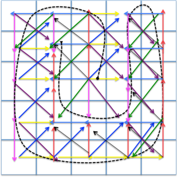
Figure 5.1. Maximum path between cells $(3,3)$ and $(2,2)$ in the $5\times 5$ grid. Each colored arrow indicates the same direction but in a different cell. All possible directions in each cell based on straight and non-overlapping criteria are shown by arrow lines. Dotted line is one of the longest possible paths without using a diagonal movement option.

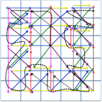
Figure 5.2. Maximum path between cells $(3,3)$ and $(1,5)$ in the $5\times 5$ grid. Each colored arrow indicates the same direction but in a different cell. All possible directions in each cell based on straight and non-overlapping criteria are shown by arrow lines. Dotted line is one of the longest possible paths using a diagonal movement option.

6. Discussion

Deconstructing movement into individual non-overlapping walks within a grid-delineated area, which may then be strung together to model the frequently repetitive, overlapping walks characteristic of the domestic chicken, provides a framework to model faecal parasite dissemination. Under the straight and non-overlapping set-up we are able to prove conditions that prevent formation of maximum walks in a $2n\times 2n$ grid (see Theorem 3.3), and in a $(2n+1)\times(2n+1)$ grid (see Theorem 3.6). In section 4, we have proved that a vector of functions of bounded variations defined on a maximum possible walk is rectifiable. By joining several rectifiable paths we arrive at more meaningful chicken walks, which mimic several realistic situations for understanding parasite transmissions. Incorporating data describing rate of defaecation (and thus parasite excretion) and previously modelled transmission rates will then be key components in construction of pathogen transmission models. Here we describe a mathematical model defining host movement, in this case a chicken but it could be any host, as the first tier of detail in the construction of a dynamic model for transmission of a pathogen which is usually not airborne, such as Eimeria. Spatial placement of a chicken in its pen or enclosure at any given time allows calculation of primary parasite dissemination, providing a tool with which the frequency of opportunities for neighbouring naive chickens to become infected may be predicted. Extension of these calculations can be used to model pathogen transmission through a flock. This approach can be adapted with relevant biological parameters for any pathogen transmitted by direct or indirect physical contact.

We have provided a framework for understanding walks of chicken. By joining several non-overlapping walks we get one complete walk of a chicken per unit time. By joining several individual non-overlapping walks, the resultant walk contains sub-walks which could be overlapped and this is close to the reality of a flock of birds in a pen. Since size of a cell within a grid is arbitrary, hence our analysis is flexible to capture walks within very small pen sizes. Informed by this framework each individual walk taken by a chicken may be portrayed across grids through diagonal as well as non-diagonal dimensions. By joining multiple paths we can define possible chicken behaviour over longer periods of time. Marrying these behavioural measures with biological data, including previously published rates of parasite transmission, we hope to develop a method of understanding pathogen transmission dynamics within the pens. One of our future aims of understanding chicken walks is to predict the presence or absence of Eimeria in a chicken and hence the proportion of infected chickens in a pen as an important step towards transmission dynamics models for Eimeria. We wish to study and build conjectures in general on association between the longest paths of bird movement and disease dynamics. Other potential applications for our chicken walk models include building age-structured graphical models for chicken walks. One of our future aims of understanding chicken walks is to predict the presence or absence of Eimeria in a chicken and hence the proportion of infected chickens in a pen as an important step towards transmission dynamics models for Eimeria. We wish to study and build conjectures in general on association between the longest paths of bird movement and disease dynamics. Other potential applications for our chicken walk models include building age-structured graphical models for chicken walks.

References

- [1] Taylor MA, Coop RL, and Wall RL Eds. Veterinary Parasitology, Blackwell Publishing Ltd. 2007.
- [2] Chapman HD, Barta JR, Blake D, Gruber A, Jenkins M, Smith N, Suo X, Tomley FM. Review of coccidiosis research. Advances in Parasitology 2013;83:93-171.
- [3] Dalloul R, Lillehoj, H. Poultry coccidiosis: recent advancements in control measures and vaccine development. Expert Review of Vaccines 2006; 5: 143–163.
- [4] Velkers FC, Bouma A, Stegeman AJ, de Jong MCM. Oocyst output and transmission rates during successive infections with Eimeria acervulina in experimental broiler flocks. Veterinary Parasitology 2012; 187:63-71.
- [5] Shirley MW, Smith AL, Tomley FM. The biology of avian Eimeria with an emphasis on their control by vaccination. Advances in Parasitology 2005; 60:285-330.
- [6] Williams RB, Johnson JD, Andrews SJ. Anticoccidial vaccination of broiler chickens in various management programmes: relationship between oocyst accumulation in litter and the development of protective immunity. Veterinary Research Communications 2000; 24:309-325.
- [7] Williams RB. Epidemiological aspects of the use of live anticoccidial vaccines for chickens. International Journal for Parasitology 1998; 28:1089-1098.
- [8] Blake DP, Billington KJ, Copestake SL, Oakes RD, Quail MA, Wan K-L, Shirley MW and Smith AL (2011) Genetic mapping identifies novel highly protective antigens for an apicomplexan parasite. PLoS Pathogens 7:e1001279
- [9] Itai A, Papadimitriou CH, Szwarcfiter JL. Hamilton paths in grid graphs. SIAM Journal on Computing 1982; 11(4): 676–686.
- [10] Zamfirescu C, Zamfirescu T. Hamiltonian properties of grid graphs. SIAM Journal on Discrete Mathematics 1992; 5(4):564–570.
- [11] Keshavarz-Kohjerdi F, Bagheri A. Hamiltonian paths in some classes of grid graphs. Journal of Applied Mathematics 2012; Article ID 475087, 17 pages, doi:10.1155/2012/475087
- [12] Kwong YH, Harris R, Rogers DG. A matrix method for counting Hamiltonian cycles on grid graphs. European Journal of Combinatorics 1994; 15(3):277–283.
- [13] Thompson GL. Hamiltonian Tours and Paths in Rectangular Lattice Graphs. Mathematics Magazine 1977; 50(3):147–150.
- [14] Nash-Williams CSJA. Infinite graphs – a survey. Journal Combinatorial Theory 1967; 3:286–301.
- [15] Nash–Williams CSJA. Reconstruction of infinite graphs. Discrete Mathematics 1991;95:221–229.
- [16] Bondy JA, Hemminger RL. Reconstructing infinite graphs. Pacific Journal of Mathematics 1974; 52:331–340.
- [17] Diestel R. Graph Theory, Springer, NY, 2000.
- [18] Harel D. Hamiltonian paths in infinite graphs. Israel Journal of Mathematics 1991; 76(3):317–336.
- [19] Rödl V, Ruciński A, Szemerédi E. Dirac-type conditions for Hamiltonian paths and cycles in 3-uniform hypergraphs. Advances in Mathematics 2011;3:1225–1299.
- [20] Bellman R. Dynamic programming treatment of the travelling salesman problem", Journal of the ACM 1962; 9: 61–63, doi:10.1145/321105.321111.
- [21] Rubin F. A Search Procedure for Hamilton Paths and Circuits", Journal of the ACM 1974; 21 (4): 576–80, doi:10.1145/321850.321854.
- [22] Ore O. Note on Hamilton circuits. American Mathematical Monthly 1960; 67:55.
- [23] Newman DJ. A problem in graph theory. American Mathematics Monthly 1958;65:611.
- [24] Kronk HV. A note on k-path Hamiltonian graphs. Journal of Combinatorial Theory 1969;7:104–106.
- [25] Ajtai M, Komlós J, Szemerédi E. The longest path in a random graph. Combinatorica 1981;1,(1), 1–12.
- [26] Pittel B. A random graph with a subcritical number of edges. Transactions of American Mathematical Society 1988; 309 (1): 51–75.
- [27] Krivelevich M, Lubetzky E, Sudakov B. Longest cycles in sparse random digraphs. Random Structures & Algorithms 2013;43(1): 1–15.
- [28] Karger D, Motwani R, Ramkumar G. On approximating the longest path in a graph, Algorithmica 1997;18 (1):82–98.
- [29] Feder T, Motwani R, Subi C, Approximating the longest cycle problem in sparse graphs, SIAM Journal on Computing 2002;31 (5):1596–1607.
- [30] Zhang WQ Liu YJ. Approximating the longest paths in grid graphs. Theoretical Computer Science 2011; 412(39): 5340–5350.
- [31] Keshavarz-Kohjerdi F, Bagheri A, Asghar AS. A linear-time algorithm for the longest path problem in rectangular grid graphs. Discrete Applied Mathematics 2012; 160(3):210-217.
- [32] Keshavarz-Kohjerdi F, Bagheri A. An efficient parallel algorithm for the longest path problem in meshes. Journal of Supercomputing 2013;65:723-741.
- [33] Fernandez de la Vega, W. Trees in sparse random graphs. Journal of Combinatorial Theory Series B 1988;45(1): 77–85.
- [34] Krivelevich M. Embedding spanning trees in random graphs. SIAM Journal of Discrete Mathematics 2010; 24 (4): 1495–1500.
- [35] Chou, Arthur W.; Ko, Ker-I On the complexity of finding paths in a two-dimensional domain. II. Piecewise straight-line paths. Electronic Notes in Theoretical Computer Science 2005 120:45-57.
- [36] Henrici P. Applied and computational complex analysis. Vol. 3. John Wiley & Sons, Inc., New York, 1986.
- [37] Cesari L. Rectifiable Curves and the Weierstrass Integral. American Mathematical Monthly 1958; 67(7):485-500.