Point bosons in a one-dimensional box:
the ground state, excitations and thermodynamics

Abstract

We determine the ground-state energy and the effective dispersion law for a one-dimensional system of point bosons under zero boundary conditions. The ground-state energy is close to the value for a periodic system. But the dispersion law is essentially different from that for a periodic system, if the coupling is weak (weak interaction or high concentration) or intermediate. We propose also a new method for construction of the thermodynamics for a gas of point bosons. It turns out that the difference in the dispersion laws of systems with periodic and zero boundary conditions does not lead to a difference in the thermodynamic quantities. In addition, under zero boundary conditions, the microscopic sound velocity does not coincide with the macroscopic one. This means that either the method of determination of $k$ in the dispersion law $E(k)$ is unsuitable or the low-energy excitations are not phonons.

I Introduction

Systems of many particles with contact interaction were studied in a lot of works, starting with the work by Bethe bethe (see other references in monographs gaudinm ; baxter1989 ; sutherland2004 and recent reviews batchelor2014 ; jiang2015 ). Models for spinless bosons with point interaction were constructed in several main works: these are the Girardeau model girardeau1960 for impenetrable particles under periodic boundary conditions (BCs), the Lieb–Liniger model ll1963 and the Lieb model lieb1963 for penetrable particles under periodic BCs, and Gaudin solutions gaudin1971 for zero BCs. Moreover, some results for the ground state under zero BCs were obtained by Batchelor et al. batchelor2005 . The influence of the boundaries on the ground state of a system of point fermions was studied as well woynarovich1985 ; batchelor2006 .

In the present work, we investigate the ground-state, the dispersion law, and the thermodynamics for spinless point bosons under zero BCs. The two following results are basic. We give a new method for construction of the thermodynamics for point bosons and find out that the dispersion law under zero BCs differs from that under periodic BCs. However, under zero BCs, the low-energy elementary excitations are not phonons, if we determine $k$ as in the present work. Therefore, the curve $E(k)$ under zero BCs is the “dispersion law” in the effective sense. The nonphononicity arouses the questions, which are considered in Section VII. The dispersion relations for $SU(2)$ point bosons under periodic and zero BCs were found in ying2001 ; ying2003 . But the results for periodic and zero BCs are given at different system parameters; therefore, it is hard to see whether dispersion relations depend on boundaries at large $N,L$.

II Initial equations

We now recall briefly the basic equations. They are presented in the elegant and exact form in the works by Gaudin gaudin1971 ; gaudinm .

Let us consider $N$ bosons, which occupy a one-dimensional (1D) interval of length $L$ and interact by means of a binary repulsive potential in the form of a delta-function. The interval can be closed or nonclosed. The Schrödinger equation for such system is usually written in the form ll1963

$$-\sum\limits_{j}\frac{\partial^{2}}{\partial x_{j}^{2}}\Psi+2c\sum\limits_{i<j}\delta(x_{i}-x_{j})\Psi=E\Psi.$$ (1)

Under periodic BCs, the solution of this equation for the domain $x_{1}\leq x_{2}\leq\ldots\leq x_{N}$ is the Bethe ansatz ll1963 ; gaudin1971

$$\Psi_{\{k\}}(x_{1},\ldots,x_{N})=\sum\limits_{P}a(P)e^{i\sum\limits_{l=1}^{N}k_{P_{l}}x_{l}},$$ (2)

where $k_{P_{l}}$ is equal to one of $k_{1},\ldots,k_{N}$, and $P$ means all permutations of $k_{l}$. The coefficients $a(P)$ were determined in lieb1963 . Under zero BCs, the solution is a superposition of plane waves (2) and all possible reflected waves gaudin1971 .

The energy of a system of point bosons

$$E=k_{1}^{2}+k_{2}^{2}+\ldots+k_{N}^{2}.$$ (3)

Since the energy is completely determined by the values of $k_{l}$, it is sufficient to find the corresponding $k_{l}$ in order to obtain the ground-state energy $E_{0}$ and the dispersion law.

For a periodic system, the equations for $k_{l}$ take the form yangs1969 ; gaudin1971

$$Lk_{i}=2\pi I^{p}_{i}-2\sum\limits_{j=1}^{N}\arctan{\frac{k_{i}-k_{j}}{c}},$$ (4)

$$I^{p}_{i}=n_{i}+i-\frac{N+1}{2},\quad i=1,\ldots,N,$$ (5)

where $n_{i}$ are integers. For the ground state, $n_{i}=0$ for all $i$. For $I^{p}_{1}<I^{p}_{2}<\ldots<I^{p}_{N},$ system (4) has the unique real solution $\{k_{i}\}$ yangs1969 . Using the equality

$$\arctan{\alpha}=(\pi/2)sgn(\alpha)-\arctan{(1/\alpha)},$$ (6)

Eqs. (4) can be rewritten in the equivalent form gaudin1971

$$Lk_{i}=2\pi n_{i}+2\sum\limits_{j=1}^{N}\arctan{\frac{c}{k_{i}-k_{j}}}|_{j\neq i}.$$ (7)

The solutions of (4) and (7) are the collections of $\{k_{i}\}$, for which $k_{j}\neq k_{i}$ for any $j\neq i$. Below, we assume the ordering $k_{1}<k_{2}<\ldots<k_{N}$, at which the equality $k_{j}=-k_{N+1-j}$ holds for the ground state.

For a system with zero BCs, the equations for $k_{l}$ take the form gaudin1971 ; gaudinm

$$L|k_{i}| = \pi n_{i}+\sum\limits_{j=1}^{N}\left(\arctan{\frac{c}{|k_{i}|-|k_{j}|}}\right.$$ (8)

$$+ \left.\arctan{\frac{c}{|k_{i}|+|k_{j}|}}\right)|_{j\neq i},\quad i=1,\ldots,N,$$

where $n_{i}$ are integers, and $n_{i}\geq 1$. With regard for (6), these equations can be written in the form

$$L|k_{i}| = \pi I^{z}_{i}-\sum\limits_{j=1}^{N}\left(\arctan{\frac{|k_{i}|-|k_{j}|}{c}}\right.$$ (9)

$$+ \left.\arctan{\frac{|k_{i}|+|k_{j}|}{c}}\right)\left.\right|_{j\neq i},\quad i=1,\ldots,N,$$

$$I^{z}_{i}=n_{i}+i-1.$$ (10)

The quantities $k_{l}$ are commonly ordered in the following way: $0<|k_{1}|<|k_{2}|<\ldots<|k_{N}|$. For brevity, we will write $k_{l}$ instead of $|k_{l}|$. In what follows, $k_{l}$ means $|k_{l}|$ everywhere under zero BCs. We denote $n=N/L$ and $\gamma=c/n$.

III Ground state of bosons in a box

For point bosons in a box, the ground state is described by Eqs. (8) – (10) with $n_{i}=1$. We can verify that $n_{i}=1$ in the following way (the strict proof is absent, as far as we know). Since $k_{1}>0$ is the smallest quasimomentum, the equation

$$Lk_{1}=\pi n_{1}+\sum\limits_{j=2}^{N}\left(\arctan{\frac{c}{k_{1}-k_{j}}}+\arctan{\frac{c}{k_{1}+k_{j}}}\right)$$

is satisfied only for $n_{1}\geq 1$. Otherwise, the right-hand side is negative, but the left-hand side must be positive. Therefore, the minimum value of $n_{1}$ is equal to $1$. The symmetry-based reasoning indicates that the ordering $k_{1}<k_{2}<\ldots<k_{N}$ assumes $n_{1}\leq n_{2}\leq\ldots\leq n_{N}$. Therefore, $n_{i}\geq 1$ for all $i$. The smallest $n_{i}$ are $n_{i}=1$. In addition, in the limit $c\rightarrow 0$ we should obtain the momenta of free particles $k_{i}=\pi/L$, which also requires $n_{i}=1$ gaudin1971 . We have studied Eq. (8) numerically by the Newton method and have found no states with the energy, which is lower then the energy of the state with $n_{i}=1$ for any $i$. We will assume that, for any $c,$ the ground state corresponds to $n_{i}=1$ for all $i$.

1) Ultraweak coupling ($c\rightarrow 0$). In this case, $|c/(k_{i}-k_{j})|\ll 1$ for all $i\neq j$. Therefore, relation (8) for the ground state changes into

$$Lk_{i}=\pi+\sum\limits_{j=1}^{N}\left(\frac{c}{k_{i}-k_{j}}+\frac{c}{k_{i}+k_{j}}\right)|_{j\neq i}.$$ (11)

Making use of the change $k_{i}=\sqrt{c/L}\cdot(q_{i}+\pi/\sqrt{cL}),$ we obtain the equation

$$q_{i}=\sum\limits_{j=1}^{N}\left(\frac{1}{q_{i}-q_{j}}+\frac{1}{q_{i}+q_{j}+2\pi/\sqrt{cL}}\right)|_{j\neq i}.$$ (12)

As $c\rightarrow 0$, we obtain

$$q_{i}=\sum\limits_{j=1}^{N}\frac{1}{q_{i}-q_{j}}|_{j\neq i}+\frac{(N-1)\sqrt{cL}}{2\pi}+O(c).$$ (13)

We set $q_{i}=q^{(N)}_{i}+(N-1)\sqrt{cL}/(2\pi)$, then

$$q^{(N)}_{i}=\sum\limits_{j=1}^{N}\frac{1}{q^{(N)}_{i}-q^{(N)}_{j}}|_{j\neq i}.$$ (14)

As was noticed by Gaudin gaudin1971 , it is the equation for roots of the Hermite polynomial $H_{N}(q)$. This can be verified by substituting the polynomial

$$H_{N}(q)=2^{N}\prod\limits_{j=1}^{N}(q-q^{(N)}_{j})$$ (15)

into the equation for the Hermite polynomials

$$\ddot{H}_{N}(q)-2q\dot{H}_{N}(q)+2NH_{N}(q)=0$$ (16)

and setting $q=q^{(N)}_{i}$. The roots $q^{(N)}_{i}$ of Hermite polynomials satisfy the relations

$$\sum\limits_{j=1}^{N}q^{(N)}_{i}=0,$$ (17)

$$\sum\limits_{j=1}^{N}\left(q^{(N)}_{i}\right)^{2}|_{N\gg 1}=N(N-1)/2+O(N^{-1})$$ (18)

(to obtain the last property, we found $q^{(N)}_{i}$ numerically for $N\leq 100$; values of $q^{(N)}_{i}$ for $N\leq 20$ are given in abramovitz1972 ). Using these formulae, we find the ground-state energy for $N\gg 1$:

$$E_{0}=\sum\limits_{i=1}^{N}k_{i}^{2}=\frac{N\pi^{2}}{L^{2}}+\frac{3(N-1)cn}{2}+\xi,$$ (19)

where $\xi$ is small. Formula (19) was previously obtained in batchelor2005 . This formula can be obtained also by algebraic transformations. In this way, we get

$$\xi=\frac{\pi c}{L^{2}}\sum\limits_{i,j=1}^{N}\frac{2k_{i}}{k_{i}-k_{j}}\left(\frac{1}{k_{i}+k_{j}}-\frac{L}{2\pi}\right)|_{j\neq i}.$$ (20)

The numerical solution of Eqs. (8) by the Newton method shows that the correction $\xi$ in (19) can be neglected if $\gamma\ll 1/N$. For $\gamma\ \lower-1.2pt\vbox{\hbox{\hbox to0.0pt{$>$\hss}\lower 5.0pt\vbox{\hbox{$\sim$}}}}\ 1/N,$ the quantity $E_{0}$ is close to the Bogolyubov solution for a periodic system: $E_{0}\approx Ncn$.

2) Weak and intermediate couplings, $N^{-1}\ \lower-1.2pt\vbox{\hbox{\hbox to0.0pt{$<$\hss}\lower 5.0pt\vbox{\hbox{$\sim$}}}}\ \gamma\ \lower-1.2pt\vbox{\hbox{\hbox to0.0pt{$<$\hss}\lower 5.0pt\vbox{\hbox{$\sim$}}}}\ 10$. In gaudin1971 , it was asserted that $E_{0}$ for a $(N,L,c)$-system with boundaries coincides with a half of the energy of the periodic $(2N,2L,c)$-system with $n_{i}=-1$ for $i=1,\ldots,N$ and $n_{i}=1$ for $i=N+1,\ldots,2N$. This is not quite so, because the first system is described by Eq. (8), whereas, for the positive quasimomenta of the second system, relation (7) yields, after the appropriate reenumeration, the equation

$$Lk_{i} = \sum\limits_{j=1}^{N}\left(\arctan{\frac{c}{k_{i}-k_{j}}}+\arctan{\frac{c}{k_{i}+k_{j}}}\right)|_{j\neq i}$$ (21)

$$+ \pi+\arctan{\frac{c}{2k_{i}}},\quad i=1,\ldots,N,$$

which differs from (8) by the term $\arctan{(c/2k_{i})}$. Therefore, there is no exact correspondence between the $(N,L,c)$-system with boundaries and the periodic $(2N,2L,c)$-system.

The value of $E_{0}$ was already calculated in gaudin1971 ; gaudinm ; batchelor2005 . But M. Gaudin and M. Batchelor et al. used a method assuming the proximity of the values of $E_{0}$ under periodic and zero BCs. However, these $E_{0}$ may strongly differ from each other. Therefore, we use a method similar to that in ll1963 , which does not require the proximity of the solution for $E_{0}$ to that under periodic BCs.

Under zero BCs, the quasimomenta $k_{i}$ satisfy Eq. (8). For $N\gg 1,$ $k_{i}$ vary smoothly as $i$ increases. Therefore, it is convenient to pass in (8) and (9) from summation to integration. Let us consider $k_{i}$ as a function of $\varsigma=i/N$: $k_{i}=\upsilon(i/N)=\upsilon(\varsigma)$. Then

$$k_{i+1}-k_{i}=N^{-1}(\partial\upsilon/\partial\varsigma)|_{\varsigma=i/N}\equiv 1/\rho(k_{i}).$$ (22)

Since $dk=d\upsilon=(d\upsilon(\varsigma)/d\varsigma)d\varsigma=(N/\rho(k))d\varsigma$, we have $d\varsigma=\rho(k)dk/N$. This yields

$$\int\limits_{k_{1}}^{k_{N}}\rho(k)dk=N\int\limits_{0}^{1}d\varsigma=N,$$ (23)

$$\sum\limits_{i=1}^{N}f(k_{i})=\frac{1}{{\scriptstyle\triangle}\varsigma}\int\limits_{0}^{1}f(\upsilon(\varsigma))d\varsigma=\int\limits_{k_{1}}^{k_{N}}f(k)\rho(k)dk,$$ (24)

where $f(k)$ is any function, and ${\scriptstyle\triangle}\varsigma=1/N$. This gives the normalization for the density of states $\rho(k)$ and the simple rule for the transition from the summation over $k_{i}$ to the integration. If we set $f(k)=1$ in (24), we obtain (23).

With regard to (24), Eq. (9) can be written in the form

$$Lk_{i}=\pi i-\int\limits_{k_{1}}^{k_{N}}\rho(k)dk\left(\arctan{\frac{k_{i}-k}{c}}+\arctan{\frac{k_{i}+k}{c}}\right)|_{k\neq k_{i}},$$ (25)

where $\ i=1,\ldots,N$, or

$$Lk_{i}-\arctan{\frac{2k_{i}}{c}}=\pi i$$

$$-\int\limits_{k_{1}}^{k_{N}}\rho(k)dk\left(\arctan{\frac{k_{i}-k}{c}}+\arctan{\frac{k_{i}+k}{c}}\right).$$ (26)

Considering $|k_{i+1}-k_{i}|$ small, we subtract the $i$th equation in (26) from the $(i+1)$th one. In view of (22), we obtain $N-1$ equations for $\rho(k_{i})$. They can be written as the integral equation

$$\pi\rho(q)-\int\limits_{k_{1}}^{k_{N}}\rho(k)dk\left(\frac{c}{c^{2}+(k-q)^{2}}+\frac{c}{c^{2}+(k+q)^{2}}\right)$$

$$=L-\frac{2c}{c^{2}+4q^{2}},$$ (27)

where $q\in[k_{1},k_{N}]$. Since $k_{1}$ is unknown and can be separated from $0$ by a gap, we write additionally the equation for $k_{1},$

$$Lk_{1}=\pi-\int\limits_{k_{2}}^{k_{N}}\rho(k)dk\left(\arctan{\frac{k_{1}-k}{c}}+\arctan{\frac{k_{1}+k}{c}}\right),$$ (28)

where $k_{2}=k_{1}+1/\rho(k_{1})$. Equations (23), (27), and (28) set the complete system of equations for $\rho(k)$, $k_{1},$ and $k_{N}$.

Let us compare them with the equations for the ground state of a periodic system. Let $N$ be even. For the positive quasimomenta $\tilde{k}_{1}<\tilde{k}_{2}<\ldots<\tilde{k}_{N/2}$ of a periodic system, the equations read

$$\int\limits_{\tilde{k}_{1}}^{\tilde{k}_{N/2}}\rho_{p}(\tilde{k})d\tilde{k}=N/2,$$ (29)

$$L\tilde{k}_{i}= -\int\limits_{\tilde{k}_{1}}^{\tilde{k}_{N/2}}2\rho_{p}(\tilde{k})d\tilde{k}\left(\arctan{\frac{\tilde{k}_{i}-\tilde{k}}{c}}+\arctan{\frac{\tilde{k}_{i}+\tilde{k}}{c}}\right)$$

$$+\pi(2i-1),\quad i=1,\ldots,N/2.$$ (30)

Equation (30) follows from (4) and (5) and yields

$$2\pi\rho_{p}(\tilde{q}) - \int\limits_{\tilde{k}_{1}}^{\tilde{k}_{N/2}}2\rho_{p}(\tilde{k})d\tilde{k}\left(\frac{c}{c^{2}+(\tilde{k}-\tilde{q})^{2}}\right.$$ (31)

$$+ \left.\frac{c}{c^{2}+(\tilde{k}+\tilde{q})^{2}}\right)=L,$$

$$L\tilde{k}_{1}= -\int\limits_{\tilde{k}_{2}}^{\tilde{k}_{N/2}}2\rho_{p}(\tilde{k})d\tilde{k}\left(\arctan{\frac{\tilde{k}_{1}-\tilde{k}}{c}}+\arctan{\frac{\tilde{k}_{1}+\tilde{k}}{c}}\right)$$

$$+\pi-2\arctan{\frac{2\tilde{k}_{1}}{c}},$$ (32)

$\tilde{k}_{2}=\tilde{k}_{1}+1/\rho_{p}(\tilde{k}_{1})$. Equations (29), (31), and (32) form the complete system of equations for a periodic system, which is written in the form of the equations for a system with boundaries. We now make changes $2\rho_{p}(\tilde{k})=\tilde{\rho}(\tilde{k})$, $\tilde{k}_{N/2}=\bar{k}_{N}$. Then the equations take the form

$$\int\limits_{\tilde{k}_{1}}^{\bar{k}_{N}}\tilde{\rho}(\tilde{k})d\tilde{k}=N,$$ (33)

$$\pi\tilde{\rho}(\tilde{q})-\int\limits_{\tilde{k}_{1}}^{\bar{k}_{N}}d\tilde{k}\left(\frac{\tilde{\rho}(\tilde{k})c}{c^{2}+(\tilde{k}-\tilde{q})^{2}}+\frac{\tilde{\rho}(\tilde{k})c}{c^{2}+(\tilde{k}+\tilde{q})^{2}}\right)=L,$$ (34)

$$L\tilde{k}_{1}= -\int\limits_{\tilde{k}_{2}}^{\bar{k}_{N}}\tilde{\rho}(\tilde{k})d\tilde{k}\left(\arctan{\frac{\tilde{k}_{1}-\tilde{k}}{c}}+\arctan{\frac{\tilde{k}_{1}+\tilde{k}}{c}}\right)$$

$$+\pi-2\arctan{\frac{2\tilde{k}_{1}}{c}},$$ (35)

$\tilde{k}_{2}=\tilde{k}_{1}+2/\tilde{\rho}(\tilde{k}_{1})$. Equation (35) can be written as

$$L\tilde{k}_{1} = \pi+A_{1}-\int\limits_{\tilde{k}_{1}+1/\tilde{\rho}(\tilde{k}_{1})}^{\bar{k}_{N}}\tilde{\rho}(\tilde{k})d\tilde{k}\left(\arctan{\frac{\tilde{k}_{1}-\tilde{k}}{c}}\right.$$ (36)

$$+ \left.\arctan{\frac{\tilde{k}_{1}+\tilde{k}}{c}}\right),$$

$$A_{1}\approx \arctan{\left(\frac{2\tilde{k}_{1}}{c}+\frac{1.5}{c\tilde{\rho}(\tilde{k}_{1})}\right)}$$

$$- 2\arctan{\frac{2\tilde{k}_{1}}{c}}-\arctan{\frac{1.5}{c\tilde{\rho}(\tilde{k}_{1})}}.$$ (37)

Equations (33), (34), (36) differ from (23), (27), (28) only by two terms. Equations (27) and Eq. (36) include the terms $-\frac{2c}{c^{2}+4q^{2}}$ and $A_{1}$, which are absent, respectively, in (34) and (28). The term $-\frac{2c}{c^{2}+4q^{2}}$ enters the combination $L-\frac{2c}{c^{2}+4q^{2}}$. As $N$ increases, the value of $L$ increases as well (at a fixed density $n$). Therefore, the quantity $-\frac{2c}{c^{2}+4q^{2}}$ gives an arbitrarily small contribution in the limit $N\rightarrow\infty.$ The quantity $A_{1}$ enters the combination $L\tilde{k}_{1}-\pi-A_{1}$. The numerical analysis shows that, in the regime $\gamma\gg 1/N^{2}$ and $N\geq 1000,$ the relations $c\tilde{\rho}(\tilde{k}_{1})\gg 1$ and $\tilde{k}_{1}/c\ll 1$ hold, from whence $|A_{1}|\ll\pi$ ($\tilde{k}_{1}$ can be estimated as $\tilde{k}_{1}\sim\tilde{k}_{N/2}/N$). In the regime $\gamma\gg 1/N,$ the relation $|A_{1}|\ll L\tilde{k}_{1}$ is valid as well. Therefore, the quantity $A_{1}$ can be neglected.

This means that, for $\gamma\gg 1/N,$ the distinction between systems (33), (34), (36) and (23), (27), (28) is negligible. Therefore, $k_{1}=\tilde{k}_{1}$, $k_{N}=\tilde{k}_{N/2},$ and $\rho(k)=\tilde{\rho}(k)=2\rho_{p}(k)$. Thus, for a system with zero BCs, $\rho(k)$ is 2 times larger and $k_{N}$ is the same, as compared with $\rho(k)$ and $k_{N}$ for a system with periodic BCs and the same $c,N,$ $L$. The contribution to $E_{0}$ is given by positive and negative $k_{i}$ under periodic BCs, and only by positive $k_{i}$ under zero BCs. Therefore, the values of $E_{0}$ under zero and periodic BCs almost coincide. The difference in these energies is small (${\scriptstyle\triangle}E\sim E_{0}/N$) and can be determined by the method gaudin1971 (see also batchelor2005 ), in which one should take the term $\arctan{(c/2k_{i})}$ into account.

We note that the same equations for zero BCs can be deduced by starting from (8).

3) Strong coupling ($\gamma\gg 1$). This case corresponds to very large $c$ or $L$. Consider Eq. (9). The limit $c\rightarrow\infty$ means large denominators on the right-hand side of (9), whereas $L\rightarrow\infty$ means small $k_{i}$, i.e., small numerators on the right-hand side of (9). In both cases, the sum on the right-hand side can be neglected. As a result, we obtain the solution

$$k_{i}=\pi i/L,$$ (38)

$$E_{0}=\sum\limits_{i=1}^{N}k_{i}^{2}=N\pi^{2}n^{2}/3.$$ (39)

The same solution for $E_{0}$ is obtained for the periodic system ll1963 . This is the Girardeau limit girardeau1960 . Formula (39) with a subsequent correction was obtained previously by another method batchelor2005 .

IV Dispersion law

IV.1 Zero boundary conditions

In order to understand the meaning of an elementary excitation for a system of point bosons with zero BCs, let us write the system of Eqs. (8) again:

$$Lk_{i} = \pi n_{i}+\sum\limits_{j=1}^{N}\left(\arctan{\frac{c}{k_{i}-k_{j}}}\right.$$ (40)

$$+ \left.\arctan{\frac{c}{k_{i}+k_{j}}}\right)|_{j\neq i},\quad i=1,\ldots,N.$$

This is a system of $N$ equations, where $n_{i}$ are integers. The ground state corresponds to $n_{i}=1$ for all $i=1,\ldots,N$. If at least one $n_{i}>1$, we have an excited state. Equations (40) can be compared with the keys of a piano. The pressing of the $l$th key can be interpreted as a generation of an elementary excitation with $n_{l}>1$. The pressing of the $j$th key ($j\neq l$) means the generation of the second elementary excitation.

By minimally pressing $l$ last keys, we obtain a configuration with $n_{i<N+1-l}=1$, $n_{i\geq N+1-l}=2$, i.e., $l$ excitations with smallest $n_{i}>1$. In work lieb1963 , such a structure is associated with a “hole,” a second type of elementary excitations. And excitations with $n_{i<N}=1,n_{N}\geq 2$ are called “particle states”lieb1963 . We note that the analysis lieb1963 was executed in another language, by starting from Eqs. (4) written for the difference $k_{i+1}-k_{i}$. However, the properties of excitations are most clearly seen from Eqs. (40). The separation of the excitations into holes and particles is based on the analogy with a Fermi system and can be carried out in the same way for periodic and zero BCs. But we consider that, for a Bose system, it is more natural to describe all excitations in a unified way. Most simply, the excitation can be associated with the clicking of a single key. In what follows, we will define the elementary excitations namely so.

We now find the dispersion law for an elementary excitation. For the ground state, we have $n_{i}=1$ for all $i$, and some $k_{i}$ are the solutions of (40). For an excited state, we write Eqs. (40) in the form

$$L\acute{k}_{i} = \pi\acute{n}_{i}+\sum\limits_{j=1}^{N}\left(\arctan{\frac{c}{\acute{k}_{i}-\acute{k}_{j}}}\right.$$ (41)

$$+ \left.\arctan{\frac{c}{\acute{k}_{i}+\acute{k}_{j}}}\right)|_{j\neq i},\quad i=1,\ldots,N,$$

where $\acute{n}_{i<N}=1$, $\acute{n}_{N}>1$. In this case, $0<\acute{k}_{1}<\acute{k}_{2}<\ldots<\acute{k}_{N}$. We set

$$\omega(k_{i})\equiv\omega_{i}=\acute{k}_{i}-k_{i}.$$ (42)

At the transition to the excited state, only the $N$th equation in (40) is changed. Therefore, we may expect lieb1963 that $\omega_{i<N}$ are small ($|\omega_{i<N}|\ll|k_{i}|$) and $\omega_{N}$ is not small. The solution agrees with this assumption. In this case, the quasimomentum and the excitation energy are as follows:

$$p=\sum\limits_{i=1}^{N}\omega_{i}=\int\limits_{k_{1}}^{k_{N-1}}\omega(k)\rho(k)dk+\omega_{N},$$ (43)

$$E=\sum\limits_{i=1}^{N}(\acute{k}^{2}_{i}-k^{2}_{i})\approx\omega^{2}_{N}+2k_{N}\omega_{N}+2\int\limits_{k_{1}}^{k_{N-1}}k\omega(k)\rho(k)dk.$$ (44)

From Eqs. (41) with the numbers $i=1,\ldots,N-1,$ we now subtract corresponding Eqs. (40). In view of the smallness of $\omega_{i<N}$ and the nonsmallness of $\omega_{N}$, we obtain the equations

$$L\omega_{i} = c\sum\limits_{j=1}^{N-1}\left\{\frac{\omega_{j}-\omega_{i}}{(k_{i}-k_{j})^{2}+c^{2}}+\frac{-\omega_{j}-\omega_{i}}{(k_{i}+k_{j})^{2}+c^{2}}\right\}|_{j\neq i}$$ (45)

$$+ f(k_{i}),$$

$$f(k_{i}) = \arctan{\frac{c}{\acute{k}_{i}-\acute{k}_{N}}}+\arctan{\frac{c}{\acute{k}_{i}+\acute{k}_{N}}}$$ (46)

$$- \arctan{\frac{c}{k_{i}-k_{N}}}-\arctan{\frac{c}{k_{i}+k_{N}}},$$

$i=1,\ldots,N-1$. The similar consideration of the $N$th equations in (40) and (41) gives the dependence $\omega_{N}(\acute{n}_{N})$, which is unnecessary for finding of $E(p)$.

In the left- and right-hand sides of (45), we add the term with $i=j$, transit from summation to integration by rule (24), and extend the domain of definition of $\omega(k)$ to negative $k$ by the rule $\omega(-k)=-\omega(k)$. Then relations (45) yield

$$\omega(q)\left(L-\frac{2c}{c^{2}+4q^{2}}\right) = c\int\limits_{-k_{N-1}}^{k_{N-1}}dk\cdot\rho(k)\frac{\omega(k)-\omega(q)}{(q-k)^{2}+c^{2}}$$ (47)

$$+ f(q),$$

$q\in[-k_{N-1},k_{N-1}]$. We expand (46) in the small parameter $\omega_{i<N}$ and obtain

$$f(q) \approx \arctan{\frac{c}{\omega_{N}+k_{N}+q}}-\arctan{\frac{c}{\omega_{N}+k_{N}-q}}$$

$$+ \arctan{\frac{c}{k_{N}-q}}-\arctan{\frac{c}{k_{N}+q}}$$

$$- \frac{\omega(q)c}{c^{2}+(\omega_{N}+k_{N}-q)^{2}}-\frac{\omega(q)c}{c^{2}+(\omega_{N}+k_{N}+q)^{2}}.$$

The sum of the first four terms in (IV.1) is larger than two last ones by a factor of $\sim|\omega_{N}/\omega(q)|\gg 1$, and the term $2c/(c^{2}+4q^{2})$ in (47) is small as compared with $L$ (for $\gamma\gg 1/N$). We neglect these three small terms.

For a periodic $(c,N,L)$-system, the relation ll1963

$$2\pi\rho_{p}(k)-L=2c\int\limits_{k_{1}=-k_{N}}^{k_{N}}dk\cdot\frac{\rho_{p}(k)}{(q-k)^{2}+c^{2}}$$ (49)

holds, where $2\rho_{p}(k)=\rho(k)$ (see the previous section). Using (22), we obtain

$$\int\limits_{-k_{N-1}}^{k_{N-1}}dk\frac{\rho(k)}{(q-k)^{2}+c^{2}}\approx\int\limits_{-k_{N}}^{k_{N}}dk\frac{\rho(k)}{(q-k)^{2}+c^{2}}$$

$$-\frac{1}{c^{2}+(q-k_{N})^{2}}-\frac{1}{c^{2}+(q+k_{N})^{2}}.$$ (50)

Equalities (49) and (50) allow us to write (47) in the form

$$\pi g(q)=c\int\limits_{-k_{N-1}}^{k_{N-1}}dk\frac{g(k)}{(q-k)^{2}+c^{2}}+f(q)+\tilde{f}(q),$$ (51)

where $g(q)=\omega(q)\rho(q),$ and

$$\tilde{f}(q)\approx\frac{c\omega(q)}{c^{2}+(q-k_{N})^{2}}+\frac{c\omega(q)}{c^{2}+(q+k_{N})^{2}},$$ (52)

$$f(q) \approx \arctan{\frac{c}{\omega_{N}+k_{N}+q}}-\arctan{\frac{c}{\omega_{N}+k_{N}-q}}$$ (53)

$$+ \arctan{\frac{c}{k_{N}-q}}-\arctan{\frac{c}{k_{N}+q}}.$$

In (51), the function $\tilde{f}(q)$ can be neglected, because $|\tilde{f}(q)|\ll|f(q)|$. Since $f(-q)=-f(q)$, relation (51) yields $g(-q)=-g(q)$. We note that the same equations are obtained, if we determine $\acute{k}_{i}-k_{i}$ from Eqs. (9) and (10).

Figure 1: Dispersion laws for point bosons for $n=1$ and 1) $\gamma=c=0.001$: the curves in the cases of zero (open circles) and periodic (open triangles) BCs and the Bogolyubov law (crosses); 2) $\gamma=c=0.1$: zero BCs (circles), periodic BCs (triangles), and the Bogolyubov law (stars).

Figure 2: Dispersion laws for $n=1$ and 1) $\gamma=c=10$: the curves in the cases of zero (open circles) and periodic (open triangles) BCs and the Bogolyubov law (crosses); 2) $\gamma=c=100$: zero BCs (circles), periodic BCs (triangles), and the Bogolyubov law (stars).

The dispersion law $E(p)$ can be obtained by formulae (43) and (44) with $k_{N-1}\approx k_{N}-1/\rho(k_{N})$, if we consider $\omega_{N}$ as a free parameter varying from $0$ to $\infty$ and, for each $\omega_{N},$ find the function $g(q)$ from Eqs. (51) and (53). The quantities $k_{N}$ and $\rho(k_{N})$ follow from the Lieb–Liniger equations for the ground state ll1963 (Eq. (23) with $\rho(k)\rightarrow\rho_{p}(k)$, $k_{1}=-k_{N}$, and Eq. (49)). Equations (51) and (53) can be easily solved numerically. For the replacement of the integral in (51) by a sum, we must merely make sure that the step is sufficiently small, so that at small $c$ the inequality $|q-k^{n}_{j}|<c$ will be valid for at least ten numerical points $k^{n}_{j}$.

The solutions for $E(p)$ are presented in Figs. 1–3 in comparison with the solutions for a periodic system lieb1963 and the Bogolyubov law bog1947 ; bz1956 for the point potential

$$E_{b}(p)=\sqrt{p^{4}+4cnp^{2}}.$$ (54)

By comparing Fig. 3 with Figs. 1 and 2, we see the dependence of $E(p)$ on $n$ for the same $\gamma$. In the limit $p\rightarrow\infty,$ all curves approach the asymptotics $E=p^{2}$. It is seen from the figures that, for $\gamma=c/n\ll 1,$ the curve for periodic BCs is close to the Bogolyubov law, but the curve for zero BCs is noticeably different from it. In particular, the effective sound velocity $(E/p)|_{p\rightarrow 0}$ for zero BCs is larger than that by Bogolyubov by $1.56$ times for $\gamma=0.001$ and $n=1;100$ and by $1.49$ times for $\gamma=0.1$ and $n=1;100$ (our numerical calculation for $\gamma=0.01$, $n=1$ gave for periodic BCs the sound velocity to be $0.97$ of the Bogolyubov one). As $\gamma$ increases, the curves for periodic and zero BCs approach each other. As $\gamma\gg 1,$ they are close to the Girardeau curve $E_{g}(p)=p^{2}+2\pi np$ girardeau1960 . The relation $\gamma\gg 1$ means $L\gg 1$ or $c\gg 1.$ It is easily seen from Eqs. (9) and (10) that, in these cases, $k_{i}\approx\pi I_{i}^{z}/L\approx\acute{k}_{i}$ for $i<N$, which yields $\omega(k)\rightarrow 0$. Therefore, we obtain from (43) and (44) $p=\omega_{N},E(p)=p^{2}+2k_{N}p$. Since $k_{N}|_{\gamma\rightarrow\infty}\rightarrow\pi n$ ll1963 , we have the Girardeau law. So, this law holds at $c=\infty$ girardeau1960 and $c\ \lower-1.2pt\vbox{\hbox{\hbox to0.0pt{$<$\hss}\lower 5.0pt\vbox{\hbox{$\sim$}}}}\ 1,\gamma\gg 1$ lieb1963 for periodic BCs and at $\gamma\gg 1$ for zero BCs.

The solution $E(p)$ for zero BCs can be written in the Bogolyubov form (54) with the replacement $c\rightarrow c\cdot\vartheta(k,c,n)$, where $\vartheta(k,c,n)$ depends weakly on $k$ and strongly on $c$ and $n$.

We note that, for $\gamma\ \lower-1.2pt\vbox{\hbox{\hbox to0.0pt{$<$\hss}\lower 5.0pt\vbox{\hbox{$\sim$}}}}\ 1$ and small or intermediate $E$ and $p,$ the main contribution to $E$ and $p$ is given by small perturbations $\omega_{i<N}$. For large $E$ and $p,$ the main contribution to these quantities is given by $\omega_{N}$. In other words, the excitations are collective for small $E$ and $p,$ and are quasi-one-particle for large $E$ and $p$. For $\gamma\gg 1,$ the excitations are quasi-one-particle for any $E$ and $p$, even for $p,\omega_{N}\rightarrow 0$. For all curves, $p_{\omega_{N}\rightarrow 0}\rightarrow 0$ for any $c$ and $n$. In Fig. 4, we show the dependence $p(\omega_{N})$ (43) under zero and periodic BCs.

Figure 3: Dispersion laws for $n=100$. 1) $c=10$, $\gamma=0.1$: the solutions in the cases of zero (open circles) and periodic (open triangles) BCs and the Bogolyubov law (crosses). 2) $c=1000$, $\gamma=10$: zero BCs (circles), periodic BCs (triangles), and the Bogolyubov law (stars).

Figure 4: Dependence $p(\omega_{N})$ (43) for $\gamma=0.001$: 1) zero BCs and $n=1$, $c=0.001$ (open circles); 2) zero BCs and $n=100$, $c=0.1$ (crosses); 3) periodic BCs and $n=1$, $c=0.001$ (circles); 4) periodic BCs and $n=100$, $c=0.1$ (stars).

IV.2 Periodic boundary conditions

The dispersion law for periodic BCs was found by E.H. Lieb lieb1963 . In order to understand the reason for the influence of boundaries on the dispersion law, let us compare the formulae obtained for zero and periodic BCs. For a periodic $(c,N,L)$-system, the equations are deduced exactly in the same way as in the case of zero BCs. Starting from Eqs. (4) and (5) or from the equivalent equation (7), we obtain

$$2\pi g_{p}(q)=2c\int\limits_{k_{1}=-k_{N}}^{k_{N}}dk\frac{g_{p}(k)}{(q-k)^{2}+c^{2}}+f_{p}(q),$$ (55)

$$f_{p}(q) \approx 2\arctan{\frac{\omega_{N}+k_{N}-q}{c}}$$ (56)

$$- 2\arctan{\frac{k_{N}-q}{c}},$$

where $g_{p}(q)=\omega(q)\rho_{p}(q)$. Equations (43) and (44) remain valid if we replace $\rho(q)\rightarrow\rho_{p}(q)$ and consider $k_{N-1}\approx k_{N}-1/\rho_{p}(k_{N})$. The values of $\rho_{p}(q)$ and $k_{N}$ can be obtained from the Lieb–Liniger equations ll1963 for the ground state of a periodic system (Eq. (23) with $\rho(k)\rightarrow\rho_{p}(k)$, $k_{1}=-k_{N}$, and Eq. (49)). In Figs. 1-3, we give the dispersion laws for periodic BCs, which were obtained numerically from Eqs. (43), (44), (55), and (56) with the indicated changes.

In the derivation of Eqs. (55) and (56), we considered $k_{1},\ldots,k_{N-1}$ to be the quasimomenta of a system of $N$ interacting atoms (like under zero BCs). Eqs. (2.18)–(2.20) from lieb1963 were obtained within another approach, where $k_{1},\ldots,k_{N-1}$ were considered to be the quasimomenta of a system of $N-1$ interacting atoms. In the first (second) approach, at $\omega_{N}>0$ we have $\omega(q)>0$ ($\omega(q)<0$). The advantage of the second approach is that the derivation of equations is simpler. However, the ground state corresponds to $N$ interacting atoms. Therefore, the first approach is slightly more exact. But the results in both approaches are very close. The first approach has the advantage that the properties $E(\omega_{N}\rightarrow 0)\rightarrow 0,p(\omega_{N}\rightarrow 0)\rightarrow 0$ follow directly from the input equations (43), (44), (55), and (56), whereas the analogous properties in the second approach are not obvious and require a bulky proof lieb1963 .

V Numerical solution by the Newton method

Trying to solve equations of the form (8) numerically, we found that this can be performed easily (for $N\ \lower-1.2pt\vbox{\hbox{\hbox to0.0pt{$<$\hss}\lower 5.0pt\vbox{\hbox{$\sim$}}}}\ 1000$) and with a high accuracy within the Newton method. This method frequently requires the proximity of a bare solution to the exact one. However, for systems (7) and (8), the method converges also with the quick choice of a bare solution. The essence of the method is as follows. Two nonlinear equations

$$f_{1}(k_{1},k_{2})=0,\quad f_{2}(k_{1},k_{2})=0$$ (57)

can be approximately written in the form

$$f_{1}(k^{(0)}_{1},k^{(0)}_{2})+\frac{\partial f_{1}}{\partial k_{1}}(k^{(0)}_{1},k^{(0)}_{2})\cdot(k_{1}-k^{(0)}_{1})$$ (58)

$$+ \frac{\partial f_{1}}{\partial k_{2}}(k^{(0)}_{1},k^{(0)}_{2})\cdot(k_{2}-k^{(0)}_{2})=0,$$

analogously for $f_{2}$. Setting $k^{(0)}_{j}=k^{(l-1)}_{j}$, $k_{j}=k^{(l)}_{j}$ ($j=1,2$), we get a linear recurrence relation between $k^{(l)}_{j}$ and $k^{(l-1)}_{j}$. Under certain conditions, the collection $\{k^{(l)}_{j}\}$ converges with increasing $l$ to the exact solution $\{k_{j}\}$.

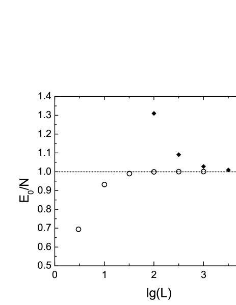
Figure 5: Dependence of $E_{0}/N$ on the system size $L$ under zero (rhombs) and periodic (circles) BCs for $n=1$, $\gamma=0.01$. The value of $E_{0}$ is obtained by direct solving of the systems of equations (7) and (8) within the Newton method. The dotted line shows the Bogolyubov solution $E_{0}/N=cn(1-4\sqrt{\gamma}/3\pi)$ taken as 1 ($E_{0}/N=1$).

By this method, we found $E_{0}$ and $E(k)$ for periodic and zero BCs by means of the direct solving of Eqs. (7) and (8). To within $1\%,$ the solutions coincide with the above-obtained ones. We get also the dependence $E_{0}(L)$ for $n=const$ (see Fig. 5). The difference in the values of $E_{0}$ for small $L$ from $E_{0}(L\rightarrow\infty)$ is the finite-size effect. The similar effect was previously studied in ying2001 ; batchelor2005 .

The Newton method is a powerful tool for solving of systems of the form (4), (7), (8), (9).

VI Thermodynamics

In the following section, we will see that the excitations are not phonons. Therefore, we cannot observe them by the scattering of some particles. It is of interest to clarify whether the difference in dispersion curves for zero and periodic BCs leads to a difference in the measured thermodynamic quantities. C.N. Yang and C.P. Yang yangs1969 constructed the thermodynamic description of point bosons, by using the mixed language of atoms and excitations (see also jiang2015 ). In particular, the free energy has the Fermi form yangs1969

$$F=N\mu-\frac{k_{B}TL}{2\pi\hbar}\int\limits_{-\infty}^{\infty}dp\ln{\left(1+e^{\frac{-\epsilon(p)}{k_{B}T}}\right)},$$ (59)

where $\epsilon(p)$ is some effective energy that is not the energy of a quasiparticle. To study the influence of the boundaries, it is necessary to carry on the whole analysis yangs1969 anew for zero BCs. However, the weakly excited state of a quantum liquid can be considered as a number of excitations and is most simply described in the language of excitations land9 . Moreover, the excitations are usually observed rather than atoms. If we separate the excitations into “holes” and “particles”, then the excitations do not obey some simple statistics. The “mixed” description was constructed yangs1969 probably just for this reason. Below, we propose a simpler way to construct the thermodynamics, which will allow us to introduce excitations in a self-consistent manner.

In what follows, the formulae are valid for zero and periodic BCs. The Gibbs canonical distribution implies that the free energy of the system reads land5

$$F=-k_{B}T\ln{\sum\limits_{j}e^{-E_{j}/k_{B}T}},$$ (60)

where $j$ enumerates all possible states of the system, and $E_{j}$ is the energy of the system in the $j$th state. Any excited state of the system is uniquely determined by the set of numbers $\{n_{i}\}\equiv(n_{1},n_{2},\ldots,n_{N})$ in (7) or (8). For the ground state, we have the set $(n^{(0)},\ldots,n^{(0)})$. Let in system (7) or (8) the number of equations with $n_{l}\neq n^{(0)}$ be much less than $N$. The analysis by the Newton method shows that, in this case, the energy of the system is

$$E(\{n_{i}\})\approx E_{0}+\sum\limits_{i=1}^{N}\varepsilon_{i}(l_{i}),$$ (61)

$$\varepsilon_{i}(l_{i})=E(n^{(0)},\ldots,n^{(0)},n_{i},n^{(0)},\ldots,n^{(0)})-E_{0},$$ (62)

where $l_{i}=n_{i}-n^{(0)}$, and $i$ is the number of the equation in system (7) or (8). Because all $i$ are equivalent, we have $\varepsilon_{i}(l_{i})=\varepsilon(l_{i})$. The quantity $\varepsilon(l_{i})$ coincides with the energy of a quasiparticle (44). $l_{i}$ can take the zero value, then $\varepsilon(0)=0$. Then relation (60) can be written in the form

$$F=E_{0}-k_{B}T\ln{\sum\limits_{l_{1}\ldots l_{N}}e^{-\sum\limits_{i=1}^{N}\varepsilon(l_{i})/k_{B}T}}.$$ (63)

In sum (63), we should take only different states into account land5 . For example, all states of the form $n_{i\neq j}=n^{(0)},n_{j}=2$ are equivalent and must be considered as a one state. It is difficult to determine such a sum (63) if $N$ is finite. However, this can be easily performed in the limit $N=\infty,L=\infty,N/L=n$. For infinite $N,$ the different states from the set $(l_{1},\ldots,l_{N})$ can be enumerated by the set of numbers $\{\eta_{l}\}$, where $\eta_{l}$ is the occupation number for the $l$th state, and $l$ has the same values as any $l_{i}$. It is also necessary to replace

$$\sum\limits_{i=1}^{N}\varepsilon(l_{i})|_{N\rightarrow\infty}\rightarrow\sum\limits_{l}\eta_{l}\varepsilon(l),$$ (64)

where the numbers $\eta_{l}$ for each $l$ can take the values $\eta_{l}=0,1,2,\ldots,\infty$. As a result, we have

$$F=E_{0}-k_{B}T\ln{\sum\limits_{\{\eta_{l}\}}e^{-\sum\limits_{l}\eta_{l}\varepsilon(l)/k_{B}T}},$$ (65)

where $\{\eta_{l}\}$ is the set $\eta_{1},\eta_{2},\ldots,\eta_{l},\ldots$ (the enumeration coincides with that one for $l$, see below). Let us rewrite $F$ in the form

$$F=E_{0}-k_{B}T\sum\limits_{l}\ln{\sum\limits_{\eta_{l}=0}^{\infty}e^{-\eta_{l}\varepsilon(l)/k_{B}T}}.$$ (66)

Summing the geometric progression, we obtain finally

$$F=E_{0}+k_{B}T\sum\limits_{l}\ln{\left(1-e^{-\varepsilon(l)/k_{B}T}\right)}.$$ (67)

This formula describes the free energy of a system of noninteracting bosons land5 with zero chemical potential and the additional summand $E_{0}$. Formula (67) indicates that the weakly excited state of a system of point bosons can be considered as a number of elementary excitations satisfying the Bose statistics.

This corresponds to the symmetry of wave functions. Indeed, the permutation of the $l$th and $j$th excitations means the permutation of $n_{l}$ and $n_{j}$ in Eq. (7) or (8). This leads only to the permutation of $k_{i}$ in the complete collection $\{k_{i}\}$. In this case, the Lieb–Liniger ll1963 and Gaudin gaudin1971 wave functions are invariable. In addition, the system can possess several excitations with identical $n_{l}$. These properties again indicates that the excitations are bosons for any $\gamma$ and $k$. By their properties, the excitations are similar to Bogolyubov ones bog1947 ; bz1956 .

We note that equality (61) holds if the total number of excitations $\ll N$, i.e., if $T$ is low. If the number of excitations is of the order of magnitude of $N$, one needs to consider their interaction.

For zero BCs, the levels are numbered as follows: $l$ can take the values $1,2,\ldots$ corresponding to the quasimomenta $k^{(l)}=(\sum\limits_{i}k_{i})|_{(n_{j\leq N-1}=1,n_{N}=l+1)}-(\sum\limits_{i}k_{i})|_{(n_{j\leq N}=1)}$. For periodic BCs, we have $l=\pm 1,\pm 2,\ldots$, $k^{(l)}=(\sum\limits_{i}k_{i})|_{(n_{j\leq N-1}=0,n_{N}=l)}-(\sum\limits_{i}k_{i})|_{(n_{j\leq N}=0)}$, $k^{(-l)}=-k^{(l)}$. By the Newton method, we determined the first $1000$ levels $(\varepsilon(l),k^{(l)})$ for periodic and zero BCs for $N=1000,n=1,$ and $\gamma=0.01;1$. It turns out that $\varepsilon_{z}(2l)=\varepsilon_{p}(l)=\varepsilon_{p}(-l)$, $\varepsilon_{z}(2l-1)=0.5(\varepsilon_{p}(l)+\varepsilon_{p}(l-1))$ (the indices $p$ and $z$ mean periodic and zero BCs, and we consider $\varepsilon_{p}(l=0)=0$). These equalities hold with accuracy $\sim 1/N$. If we neglect the small difference $\varepsilon_{p}(l)-\varepsilon_{p}(l-1)$, we obtain $\varepsilon_{z}(1)=\varepsilon_{p}(-1),\ \varepsilon_{z}(2)=\varepsilon_{p}(1),\ \varepsilon_{z}(3)=\varepsilon_{p}(-2),\ \varepsilon_{z}(4)=\varepsilon_{p}(2),$ and so on. In other words, the energies of levels under periodic and zero BCs coincide. Therefore, the free energies (63) for the systems under periodic and zero BCs are identical. With regard to the difference $\varepsilon_{p}(l)-\varepsilon_{p}(l-1)$, we obtain a surface correction $\sim F/N$ to the free energy $F$.

In (67), we may pass to the integration with respect to $p$ or $E$:

$$F\approx E_{0}+\frac{k_{B}TL}{2\pi\hbar}\int\limits_{-\infty}^{\infty}dp\zeta(p)\ln{\left(1-e^{\frac{-E(|p|)}{k_{B}T}}\right)},$$ (68)

$$F\approx E_{0}+\frac{k_{B}TL}{2\pi\hbar}\int\limits_{-\infty}^{\infty}dE\tilde{\zeta}(E)\ln{\left(1-e^{\frac{-E}{k_{B}T}}\right)},$$ (69)

where $\zeta(p_{l})=2\pi[L(k^{(l+1)}-k^{(l)})]^{-1}$ for periodic BCs and $\zeta(p_{l})=\pi[L(k^{(l+1)}-k^{(l)})]^{-1}$ for zero BCs, $p_{l}=\hbar k^{(l)}$, $\tilde{\zeta}(E)=\zeta(p)\cdot\partial p/\partial E$. For zero BCs, $\zeta(-|p|)\equiv\zeta(|p|)$. The numerical analysis indicates that, for periodic BCs, $k^{(l+1)}-k^{(l)}=2\pi/L$ and $\zeta(p)=1$. For zero BCs, the step $k^{(l+1)}-k^{(l)}$ depends on $l$ and differs from the step for periodic BCs (which leads to the different dispersion law). In this case, $\tilde{\zeta}(E)$ is the same under periodic and zero BCs with deviation $\ \lower-1.2pt\vbox{\hbox{\hbox to0.0pt{$<$\hss}\lower 5.0pt\vbox{\hbox{$\sim$}}}}\ 0.3\%$. Therefore, relation (69) allows us again to conclude that $F$ is independent of the boundaries.

Formula (68) with $\zeta(p)=1$ describes the free energy of a gas of excitations in He II xal (with the additional term $E_{0}$ independent of $T$).

It is of interest that the total number of excitations in a gas of point particles is at most $N,$ by definition. For a gas of nonpoint particles, the excitation is manifested as a multiplier of the total wave function bz1956 ; fc ; yuv1980 ; zero-liquid , and the number of multipliers is unbounded. Moreover, the system of energy levels of $N$ point particles has no level corresponding to $N+1$ phonons in a gas of $N$ nonpoint particles. That is, some states of a gas of nonpoint particles have an analog in a gas of point particles, whereas another states do not have. Intuitively it seems that a real system of $100$ Bose particles can hold $150$ oscillatory waves (phonons). It is possible that, for finite $N,$ the excitations for point particles are defined not quite self-consistently.

VII Nature of excitations, open questions

We have shown above that, for a weak and intermediate couplings, the dispersion law for point bosons does depend on the presence of boundaries, whereas the ground-state energy is independent of boundaries (to within the surface correction $\sim E_{0}/N$). Why is it so as regards equations? As was shown in Sec. III, the equations for the ground state for systems with zero and periodic BCs differ from each other only by two terms, which are small for large $N$ and $L$. But the equations for the dispersion law differ from each other strongly. Namely, for periodic BCs, the functions $f_{p}(q)$ and $g_{p}(q)$ in Eqs. (55), (56) are constant-sign for all $q$. But, under zero BCs, $f(-q)=-f(q)$ and $g(-q)=-g(q)$ (see Eqs. (51), (53)). Thus, the equations under periodic and zero BCs differ by their symmetries. Therefore, the solutions for the dispersion laws are also different.

However, for zero BCs, the low-lying excitations are not phonons. In order to see this, let us compare the microscopic sound velocity $v_{s}^{micro}=\partial E(p)/\partial p|_{p\rightarrow 0}$ with the macroscopic one $v_{s}^{macro}=\sqrt{\partial P/\partial\rho},P=-\partial E_{0}/\partial V$ $(\rho=mn)$ putterman . Under the periodic BCs, they are identical girardeau1960 ; lieb1963 . Therefore, the excitations with small $p$ can be interpreted as phonons. Under zero BCs, the system is characterized by the same $E_{0}$ and $v_{s}^{macro}$, but by the different value of $v_{s}^{micro}$, being approximately $1.5$ times over $v_{s}^{macro}$ at $\gamma\ll 1$. Hence, under zero BCs, the excitations with small $p$ are not phonons. This is true for $\gamma\ \lower-1.2pt\vbox{\hbox{\hbox to0.0pt{$<$\hss}\lower 5.0pt\vbox{\hbox{$\sim$}}}}\ 10$. For $100\ \lower-1.2pt\vbox{\hbox{\hbox to0.0pt{$<$\hss}\lower 5.0pt\vbox{\hbox{$\sim$}}}}\ \gamma<\infty,$ the relation $v_{s}^{micro}\approx v_{s}^{macro}$ holds, and the excitations are almost phonons. For $\gamma=\infty,$ we have $v_{s}^{micro}=v_{s}^{macro}$, and the excitations can be considered as phonons. Which structure of the wave function (WF) under zero BCs should be in order that an excitation be a phonon? The total WFs are not eigenfunctions of the operator of total momentum even for $\gamma=\infty$. But the WF can contain a multiplier corresponding to two counter-propagating waves. In this case, the WF of a low-energy state should have the form

$$\Psi(x_{1},\ldots,x_{N})=(\psi(x_{1},\ldots,x_{N}|k)+\psi(x_{1},\ldots,x_{N}|-k))\Psi_{0},$$ (70)

where the function $\psi(x_{1},\ldots,x_{N}|k)$ is an eigenfunction of the total operator of momentum with the eigenvalue $k$. The structure of (70) is phonon-like. If such representation is possible, then the excited state has the phonon structure and is characterized by the quasimomentum $k$. In this case, the relation $v_{s}^{micro}=v_{s}^{macro}$ should hold. But since $v_{s}^{macro}$ is the same as for periodic BCs, the dispersion law $E(k)$ should coincide with that for a periodic system. We do not know whether a representation of the form (70) exists.

According to solutions zero-liquid ; zero-gas , the boundaries of a system of nonpoint bosons affect both the dispersion law and the ground-state energy. For a 1D system of almost point bosons with the weak interaction and zero BCs, the following dispersion law is found zero-liquid ; zero-gas :

$$E(p)=\sqrt{p^{4}+2cnp^{2}}.$$ (71)

For the solutions zero-liquid , the equality $v_{s}^{micro}=v_{s}^{macro}$ holds; this can be verified for the weak coupling. The dispersion law (71) is characterized by the sound velocity, which is $\sqrt{2}$ times less than the Bogolyubov one (see (54)). However, for the point bosons in a box, the effective $v_{s}^{micro}$ is larger than the Bogolyubov $v_{s}$. If there exists a continuous transition from a nonpoint interaction to the point one, then the noncoincidence of solutions zero-liquid with those for point bosons indicates the incorrectness of either solutions zero-liquid or the solutions of the present work. However, we solved the Gaudin equations for $k_{i}$ by two different methods and are sure in the validity of the solutions. In addition, if there is no phonon representation for excitations of a gas of point bosons under zero BCs, we are faced with the difficulty for the theory of point bosons. Indeed, for the real quantum Bose liquids, the low-lying excitations are phonons. This is testified, for example, by the experiments on the scattering of neutrons and by the measurements of the heat capacity of 3D He II in a vessel (zero BCs). The distinction of the one- and three-dimensional cases should not be important, because several microscopic models of He II bz1956 ; fc ; yuv1980 ; zero-liquid work in 1D and 3D and give for 1D and 3D the solutions of the same structure.

As a possible reason for all disagreements, we can indicate the absence of a continuous transition from a nonpoint interaction to the point one, i.e., the anomality of the $\delta$-function. The $\delta$-function is a singular generalized function. It is commonly accepted that the replacement of a real potential by the $\delta$-function is admissible. In particular, it was proved mathematically seiringer2008 that the energy levels of a system of 3D bosons in a very extended trap are close to those of the Lieb–Liniger problem. However, the wave functions of $N$ nonpoint and $N$ point particles have different forms zero-liquid . Is it the different forms of the same functions or the evidence of the difference of the functions? It is known only girardeau1960 that, under periodic BCs, the WFs of point bosons with $\gamma=\infty$ can be written as the zero approximation for the WFs of nonpoint bosons. It is necessary to show that, for an $N$-particle 1D system, all energy levels and the WFs for the almost point and point interactions coincide. In the Appendix, this is proved for the one-particle problem. The same should be proved at least for $N=2$ as well. It is of interest that, in the 2D- and 3D-spaces, the potential $\delta(\textbf{x})$ has no influence on the solutions of the Schrödinger equation for some tasks simenog2014 .

The equations for spin systems and point bosons are similar gaudinm . Therefore, one can expect that the dispersion laws of spin waves under zero and periodic BCs should be different (by our method of determination of $k$), whereas the thermodynamic quantities should coincide. From whence, we may conclude that the difference of the curves $E(k)$ is unobservable. But it was shown in experiments on the scattering of neutrons that the low-lying excitations of magnetics with boundaries (zero BCs) are quite observable and have quasimomentum. The possible reason is that the spin wave is accompanied by the sound wave. An important point is that the contact Hamiltonian describes well the real exchange interaction and contains no $\delta$-function. Therefore, the solutions should correspond to the natural properties, and disagreements due to the $\delta$-function should not arise. Such a deductive method indicates that the problems of solutions for spin waves and point bosons under zero BCs are not, apparently, related to the $\delta$-function.

VIII Conclusion

We have obtained two main results: 1) It is found that the dispersion law $E(k)$ of a system of point bosons depends strongly on boundaries in the regimes of weak and intermediate coupling. 2) The thermodynamics of a gas of point bosons is constructed by a new method. Our analysis shows that the values of thermodynamic quantities are independent of the boundaries. By our method of determination of the quasimomentum $k$ of an excitation, it turns out that, under zero BCs, the low-energy excitations are characterized by a linear dispersion law and a nonphonon structure of the wave function. It seems strange, because the experiment indicates that the low-lying excitations of real uniform quantum liquids with zero boundary conditions are phonons. It is possible that there exists a way of determination of $k$ under zero BCs, for which the low-energy excitations are phonons. Otherwise, the solutions for point bosons do not describe the real low-lying modes, and we meet an internal difficulty of theory.

The author is grateful to Yu. V. Shtanov for the discussion and the indication of an error in the analysis of the $\delta$-function. I also thank the referees for helpful remarks.

IX Appendix. Comparison of the solutions for point and almost point potentials

The interatomic potentials $U(r)$ are usually have a high repulsive barrier in the region $r\ \lower-1.2pt\vbox{\hbox{\hbox to0.0pt{$<$\hss}\lower 5.0pt\vbox{\hbox{$\sim$}}}}\ 2\,\mbox{\AA}$ and a shallow pit in the region $2\,\mbox{\AA}\ \lower-1.2pt\vbox{\hbox{\hbox to0.0pt{$<$\hss}\lower 5.0pt\vbox{\hbox{$\sim$}}}}\ r\ \lower-1.2pt\vbox{\hbox{\hbox to0.0pt{$<$\hss}\lower 5.0pt\vbox{\hbox{$\sim$}}}}\ 5\,\mbox{\AA}$ and tend asymptotically to zero, as $r$ increases szalewicz2012 . Is it possible to model a nonpoint high barrier with the $\delta$-function? To answer, we compare the solutions for the wave functions and the energies obtained for both potentials.

Here, we consider the simplest one-particle task: a particle in the one-dimensional potential well $-L/2\leq x\leq L/2$ (i.e., zero BCs at $x=\pm L/2$) with the potential barrier

$$U(|x|)=\left[\begin{array}[]{ccc}\bar{U}=R_{0}U_{0}/a>0,&\ |x|\leq a,&\\ 0,&\ |x|>a&\end{array}\right.$$ (72)

at the well center. Here, $a\ll L/2$. The Fourier transform of such potential is $\nu(k)=(2R_{0}U_{0}\sin{ak})/ak$. By passing to the limit $a\rightarrow 0,$ we have $\nu(k)\rightarrow 2R_{0}U_{0}=2c=const$, which corresponds to $U(x)=2c\delta(x)$. Let us compare the solutions for almost point (arbitrarily small, but finite $a$) and point interactions.

The Schrödinger equation reads

$$-\Psi^{\prime\prime}(x)+U(x)\Psi(x)=E\Psi(x).$$ (73)

At a finite $a,$ we seek a solution in the form

$$\Psi(x)=\left[\begin{array}[]{ccc}b_{1}\cos{kx}+b_{2}\sin{kx},&x\in[-L/2,-a[,&\\ d_{1}e^{-\kappa x}+d_{2}e^{\kappa x},&\ |x|\leq a,&\\ a_{1}\cos{kx}+a_{2}\sin{kx},&\ x\in]a,L/2].&\end{array}\right.$$ (74)

Relation (73) yields $E=k^{2},\kappa=\sqrt{\bar{U}-k^{2}}$ (for $|k|\leq\sqrt{\bar{U}}$). The boundary conditions and the sewing conditions for $\Psi(x)$ and $\Psi^{\prime}(x)$ yield the equations

$$b_{1}\cos{(kL/2)}-b_{2}\sin{(kL/2)}=0,$$ (75)

$$a_{1}\cos{(kL/2)}+a_{2}\sin{(kL/2)}=0,$$ (76)

$$b_{1}\cos{ka}-b_{2}\sin{ka}=d_{1}e^{\kappa a}+d_{2}e^{-\kappa a},$$ (77)

$$b_{1}k\sin{ka}+b_{2}k\cos{ka}=-\kappa d_{1}e^{\kappa a}+\kappa d_{2}e^{-\kappa a},$$ (78)

$$a_{1}\cos{ka}+a_{2}\sin{ka}=d_{1}e^{-\kappa a}+d_{2}e^{\kappa a},$$ (79)

$$-a_{1}k\sin{ka}+a_{2}k\cos{ka}=-\kappa d_{1}e^{-\kappa a}+\kappa d_{2}e^{\kappa a}.$$ (80)

They have two “branches” of solutions. For $a\rightarrow 0$ and $k^{2}\ll\bar{U},$ we have
I) $d_{1}=d_{2}=a_{1}/2$, $b_{1}=a_{1}$, and $b_{2}=-a_{2}=a_{1}/\tan{(kL/2)}.$ The value of $a_{1}$ can be found from the normalization condition, and $k$ satisfies the equation

$$\tan{(kL/2)}=-k/c.$$ (81)

II) $d_{1}=-d_{2}=-ka_{2}/2\kappa\rightarrow 0$, $b_{1}=-a_{1}=0$, $b_{2}=a_{2}$, $a_{2}$ is determined from the normalization condition, and $k$ satisfies the equation

$$\tan{(kL/2)}=0,\ k=2\pi l/L,\ l=1,2,3,\ldots$$ (82)

For the point potential $U(x)=2c\delta(x),$ we seek the solution of Eq. (73) in the form (LABEL:4-3) without the second row. We possess the BCs

$$\Psi(\pm L/2)=0,$$

the condition of continuity of $\Psi(x)$ at the point of the barrier

$$\Psi(x=-\delta)|_{\delta\rightarrow 0}=\Psi(x=\delta)|_{\delta\rightarrow 0},$$

and the equation

$$[\Psi^{\prime}(x=\delta)-\Psi^{\prime}(x=-\delta)]|_{\delta\rightarrow 0}=2c\Psi(0),$$ (83)

obtained by the integration of the Schrödinger equation (73) on the interval $x\in[-\delta,\delta]$ (a similar equation arises also for $N$ point bosons ll1963 ). These equations have two branches of the solutions: 1) $E=k^{2}$, $b_{1}=a_{1}$, $b_{2}=-a_{2}=a_{1}/\tan{(kL/2)}$, and Eq. (81) for $k$; 2) $E=k^{2}$, $b_{1}=a_{1}=0$, $b_{2}=a_{2}$, and Eq. (82) for $k$. They coincide with solutions (I) and (II) for almost point particles. We note that though the function $\delta(x)$ does not act on odd functions, such functions can be eigenfunctions of the Hamiltonian with the $\delta$-function.

Let us consider the properties of solutions. For series (I), the lower level corresponds to the WF without nodes. The next levels correspond to the WFs with two, four, etc nodes. For series (II), the lower level corresponds to the WF with a single node. For the next levels, the WFs have three, five, etc nodes. By the theorem of nodes gilbert , the ground state corresponds to the WF without nodes, the first excited state to the WF with one node, the second excited state to the WF with two nodes, etc. Solutions (I) and (II) correspond to the theorem of nodes.

Note that the eigenvalue $E=k^{2}$ of the Schrödinger equation coincides with the value of $\langle\Psi_{0}|\hat{H}|\Psi_{0}\rangle$ both for the almost point interaction and for the point one. In the proof, it is necessary to consider that, for the point potential, $\Psi_{0}^{\prime}(x)$ has a discontinuity at the point $x=0$ (see (83)).

- (1) H.A. Bethe, Z. Phys. 71, 205 (1931).
- (2) M. Gaudin, La Fonction d’Onde de Bethe (Masson, Paris, 1983; Mir, Moscow, 1987).
- (3) R.J. Baxter, Exactly Solved Models in Statistical mechanics (Academic Press, London, 1989).
- (4) B. Sutherland, Beautiful models. 70 Years of Exactly Solved Quantum many-body problems (World Scientific, Singapore, 2004).
- (5) M.T. Batchelor, Int. J. Mod. Phys. B 28, 1430010 (2014).
- (6) Y.-Z. Jiang, Y.-Y. Chen, and X.-W. Guan, Chin. Phys. B 24, 050311 (2015).
- (7) M. Girardeau, J. Math. Phys. (N.Y.) 1, 516 (1960).
- (8) E.H. Lieb and W. Liniger, Phys. Rev. 130, 1605 (1963).
- (9) E.H. Lieb, Phys. Rev. 130, 1616 (1963).
- (10) M. Gaudin, Phys. Rev. A 4, 386 (1971).
- (11) M.T. Batchelor, X.W. Guan, N. Oelkers, C. Lee, J. Phys. A 38, 7787 (2005).
- (12) F. Woynarovich, Phys. Lett. 108A, 401 (1985).
- (13) N. Oelkers, M.T. Batchelor, M. Bortz, X.-W. Guan, J. Phys. A 39, 1073 (2006).
- (14) S.J. Gu, Y.Q. Li, Z.J. Ying, J. Phys. A 34, 8995 (2001).
- (15) Y.Q. Li, S.J. Gu, Z.J. Ying, U. Eckern, EPL 61, 368 (2003).
- (16) C.N. Yang and C.P. Yang, J. Math. Phys. (N.Y.) 10, 1115 (1969).
- (17) Handbook of Mathematical Functions, Ed. by M. Abramovitz and I.A. Stegun (U.S. Department of Commerce, Washington, 1972), Chap. 25, p. 924.
- (18) N.N. Bogoliubov, J. Phys. USSR 11, 23 (1947).
- (19) N.N. Bogoliubov and D.N. Zubarev, Sov. Phys. JETP 1, 83 (1956).
- (20) E.M. Lifshitz and L.P. Pitaevskii, Statistical Physics, Part 2 (Pergamon Press, Oxford, 1980; Nauka, Moscow, 2002), Chap. 7.
- (21) L.D. Landau and E.M. Lifshitz, Statistical Physics, Part 1 (Pergamon Press, Oxford, 1980; Nauka, Moscow, 2002), Chap. 3, 5.
- (22) I.M. Khalatnikov, An Introduction to the Theory of Superfluidity (Perseus, Cambridge, 2000), Chapter 1.
- (23) R.P. Feynman and M. Cohen, Phys. Rev. 102, 1189 (1956).
- (24) I.A. Vakarchuk and I.R. Yukhnovskii, Theor. Math. Phys. 42, 73 (1980).
- (25) M.D. Tomchenko, Ukr. J. Phys. 59, 123 (2014).
- (26) S.J. Putterman, Superfluid Hydrodynamics (American Elsevier Publ. Co., New York, 1974), Chap. 1.
- (27) M. Tomchenko, arXiv:cond-mat/1204.2149.
- (28) R. Seiringer, J. Yin, Commun. Math. Phys. 284, 459 (2008).
- (29) I.V. Simenog, B.E. Grinyuk, M.V. Kuzmenko, Ukr. J. Phys. 59, 1177 (2014).
- (30) W. Cencek, M. Przybytek, J. Komasa, J.B. Mehl, B. Jeziorski, and K. Szalewicz, J. Chem. Phys. 136, 224303 (2012).
- (31) R. Courant and D. Hilbert, Methods of Mathematical Physics (Interscience, New York, 1949), Vol. 1, Chap. 6.