Trapping Spin-$0$ particles on $p-$balls in $(D,1)$ dimensions

Abstract

p-Balls are topological defects in $(D,1)$ dimensions constructed with $\mathcal{M}\geq 1$ scalar fields which depend radially on only $2\leq p\leq D-2$ spatial dimensions. Such defects are characterized by an action that breaks translational invariance and are inspired on the physics of a brane with $D-p$ extra dimensions. Here we consider the issue of localization of bosonic states described by a scalar field $\Phi$ sufficiently weak to not disturb sensibly the defect configuration. After describing the general formalism, we consider some specify examples with $\mathcal{M}=1,2$ and $3$, looking for some region of parameters where bound and resonant bosonic states can be found. We investigate the way the influence of the defect structure, number of radial dimensions and coupling between the fields are related to the occurrence of bound and resonant states.

I Introduction

The study of topological defects vilenkin ; sutcliffe is important due to their mathematical properties and connection to several areas of physics such as quark confinement phenom , cosmology cosm and condensed matter condmat . From the point of view of multidimensional spacetimes, one can cite for instance the vortex vortex for superconductor physics in $(2,1)$ dimensions, the magnetic monopole monopole connected to cosmology in $(3,1)$ dimensions and brane models brane-origins in general $(p,1)$ dimensions. The simplest example of a topological defect is the kink kink , where the solution interpolates between two different vacua. The kink is extended by the concept of branes with one extra dimension thick1 ; thick2 ; thick3 ; thick4 ; thick5 ; thick6 ; thick7 ; thick8 ; thick9 ; thick10 ; thick_rev , where the brane structure is a result of an action with a dynamical scalar field. The tentative of solving the hierarchy and the constant cosmological problems with one extra dimension always faced a fine-tuning problem brane-origins . Some tentative to evade this problem included to consider more than one extra dimension. The literature has several interesting examples of topological defects with larger codimension number. In 6 dimensions with codimension 2 one can cite gravity localization on strings 6dim and baby-Skyrmion branes skyr . Higher codimension topological defects are studied in highercodim .

In general codimension-1 brane models can be easily treated using the first-order formalism thick1 . In such cases the scalar field potential and metric can be described by first-order differential equations in terms of a function $W$ called fake superpotential. This name refers to the flat spacetime analog where a true superpotential is introduced to find BPS states bps . The BPS formalism for some defects with radial symmetry constructed with a scalar field was introduced in Refs. bmm1 ; bmm2 . Recently, inspired in brane models with codimension-2, such study was extended for the case of two coupled scalar fields in $(3,1)$-dimensions with the aim to investigate in absence of gravity resonances and localization of particles with spin-$0$ tube_scalar and spin-$1/2$ tube_fermion in axial symmetric topological defects. Such analysis has shown similar results with the previous works dealing with gravity and particle localization and resonances brane_ress on branes with codimension 1.

In presence of gravity, the lack of a first-order formalism for brane-models with codimension higher than 1 make the analysis of field localization and resonance much more involved, needing in general numerical analysis for finding the way the scalar fields depend on the extra dimensions. However, by neglecting gravity effects, in this work we show that is possible to implement a first-order formalism to describe topological defects generated by scalar fields with pure radial dependence. Consequently, we analyze the effects in the trapping of spin-$0$ fields due to the higher codimension of the topological defect.

This paper is presented in the following way: In Section II we consider the general fist-order formalism for a $(D,1)-$dimensional flat spacetime where $\mathcal{M}\geq 1$ scalar fields depend radially on $p$ spatial dimensions, with $2\leq p\leq D-2$. Next we apply the formalism for a certain number of specific cases. Then, in Sects III, IV and V we consider defects formed respectively by one, two and three field models, looking for some aspects of localization of a spin-0 field in each system, and numerically investigating the occurrence of bound states and resonance effects. Our main conclusions concerning to a comparative analysis of the influence of $p$, $D$ and $\mathcal{M}$ on the number and intensity of resonances are presented in Sect. VI.

II General formalism

We start with the action

$$S=\int dtd^{D}x\bigg{(}\sum_{i=1}^{\mathcal{M}}\frac{1}{2}\partial_{\alpha}\phi^{i}\partial^{\alpha}\phi^{i}-V(\phi^{1},...,\phi^{\mathcal{M}})\bigg{)}$$ (1)

with $\alpha=0,...,D$. The $(D,1)$-dimensional cartesian coordinates will be separated in $D-p$-dimensions $(x^{1},x^{2},...,x^{D-p})$ where the fields can be located and the remaining $p$ transverse dimensions $(x^{D-p+1},...,x^{D})$, with $2\leq p\leq D-2$, where the defect will be formed.

The potential is chosen to be

$$V(\phi^{1},...,\phi^{\mathcal{M}})=\frac{1}{2r^{N}}\sum_{i=1}^{\mathcal{M}}\left(W_{\phi^{i}}\right)^{2},$$ (2)

where we have used a simplified notation:

$$W_{\phi_{i}}=\frac{\partial W}{\partial{\phi_{i}}},~{}W_{\phi_{i}\phi_{j}}=\frac{\partial^{2}W}{\partial\phi_{i}\partial\phi_{j}},$$ (3)

and so on. The explicit dependence of the potential on $r$,

$$r=\sqrt{\sum_{i=D-p+1}^{D}(x^{i})^{2}},$$ (4)

follows closely and generalizes for $\mathcal{M}$ scalar fields the construction of Ref. bmm1 ; bmm2 , initially motivated for avoiding the Derrick-Hobart’s theorem Hob -Raj . We also suppose that the scalar fields $\phi^{i}$ depend only on $r$.

The equations of motion for the scalar fields read

$$\square\phi^{i}+\frac{1}{r^{N}}\sum_{j=1}^{\mathcal{M}}W_{\phi^{j}}W_{\phi^{j}\phi^{i}}=0,\;\;i=1,...,\mathcal{M},$$ (5)

and the ones describing static solutions are

$$\nabla^{2}\phi^{i}=\frac{1}{r^{N}}\sum_{j=1}^{\mathcal{M}}W_{\phi^{j}}W_{\phi^{j}\phi^{i}},\;\;i=1,...,\mathcal{M},$$ (6)

where $\nabla^{2}$ is the $p-$dimensional Laplacian, defined by

$$\nabla^{2}\phi^{i}=\frac{1}{r^{p-1}}\frac{d}{dr}\left(r^{p-1}\frac{d\phi^{i}}{dr}\right).$$ (7)

The energy density is given by

$$\rho(r)=\frac{1}{2}\sum_{i=1}^{\mathcal{M}}\left[\left(\nabla\phi^{i}\right)^{2}+\frac{1}{r^{N}}\left(W_{\phi^{i}}\right)^{2}\right],$$ (8)

and the total energy of the defect in the transverse volume is

$$E=\int dx^{D-p+1}...dx^{D}\,\rho(r).$$ (9)

In order to describe the system via first-order differential equations, we implement the BPS formalism such that the total energy can be written as

$$E=\frac{2\pi^{p/2}}{\Gamma(p/2)}\frac{1}{2}\sum_{i=1}^{\mathcal{M}}\int dr~{}r^{p-1}\left[\left(\frac{d\phi^{i}}{dr}\mp\frac{1}{r^{N/2}}W_{\phi^{i}}\right)^{2}\pm\frac{2}{r^{N/2}}\frac{d\phi^{i}}{dr}W_{\phi^{i}}\right].$$ (10)

By setting as null the squared term we get the set of first-order differential equations

$$\frac{d\phi^{i}}{dr}=\pm\frac{1}{r^{N/2}}W_{\phi^{i}},i=1,...,\mathcal{M},$$ (11)

whose solutions we label as $\phi_{\pm}^{i}(r)$. Whenever these first-order equations are satisfied and using (3), the total energy reads

$$E=\pm\frac{2\pi^{p/2}}{\Gamma(p/2)}\sum_{i=1}^{\mathcal{M}}\int dr~{}r^{p-1}\frac{1}{r^{N/2}}\frac{dW}{dr}.$$ (12)

At this point we observe the integrand can be transformed in a total derivative whether $N=2p-2$. In this way the BPS energy reads

$$E_{{}_{BPS}}=\frac{2\pi^{p/2}}{\Gamma(p/2)}|W(r\rightarrow\infty)-W(r=0)|,$$ (13)

and from Eq. (11) the corresponding BPS equations read

$$\frac{d\phi^{i}}{dr}=\pm\frac{1}{r^{p-1}}W_{\phi^{i}},i=1,...,\mathcal{M}.$$ (14)

A similar result about parameter $N$ can be obtained by considering scaling properties of the scalar fields in the energy density (9). Firstly, we define the vectors $\vec{\phi}=(\phi^{1},...,\phi^{\mathcal{M}})$ and $\vec{r}=(x^{D-p+1},...,x^{D})$. We make the scaling transformation $\vec{r}\to\lambda\vec{r}$ and $\vec{\phi}(\vec{r})\to\vec{\phi}(\lambda\vec{r})$, corresponding to a change in the energy given by $E\to E^{\lambda}$, and impose $(\partial E^{\lambda})/(\partial\lambda)|_{\lambda=1}=0$. This leads to the following restrictions on $N$ and $p$: i) for $p=1$, $N=0$; ii) for $p=2$, $N=2$. Additionally by imposing the equality of the gradient and potential parts of $E$, we get iii) for $p\geq 3$, $N=2p-2$. A similar result was previously found in bmm1 , for the case where $D=p$.

Hence, we have shown the system (6) admits topological solutions obtained from the set of self-dual equations (14) which minimize the system energy (9).

The topological character of the solutions $\phi^{i}_{\pm}$ can be demonstrated following closely Ref. bmm1 , with the difference that there one has $p=D$. For $(1,1)$-dimensions we have $\mathcal{M}$ conserved currents $j^{i\mu}=\epsilon^{\mu\nu}\partial_{\nu}\phi^{i}$, with $\mu=0,1$ and $i=1,...\mathcal{M}$. This results in $\mathcal{M}$ conserved quantities $\sigma^{i}=d\phi^{i}/dx$, such that $\rho=\sum_{i}(\sigma^{i})^{2}$ is the energy of the field configuration bbrito and the topological charge $Q_{T}=\int_{-\infty}^{\infty}dx\rho$ is also the total energy of the solution. However, for the class of defects described here one must be in $(D,1)$-dimensions with $D\geq 4$, with the scalar fields depending on $p\geq 2$ spatial dimensions. For the minimum case, with $D=4$ and $p=2$ we have $\mathcal{M}$ current tensors $j^{i\mu_{1}\mu_{2}}=\epsilon^{\mu_{1}\mu_{2}\mu_{3}}\partial_{\mu_{3}}\phi^{i}$, where each $\mu_{1},\mu_{2},\mu_{3}$ can assume the values $0,1,2$. We have $\partial_{\mu_{1}}j^{i\mu_{1}\mu_{2}}=0$. For each scalar field this gives the set of two conserved densities $\sigma^{ik_{1}}=j^{i0k_{1}}$, where $k_{1}=1,2$. The scalar quantity $\rho=\sigma_{ik_{1}}\sigma^{ik_{1}}=j_{i0k_{1}}j^{i0k_{1}}=\epsilon_{i0k_{1}k_{2}}\epsilon^{i0k_{1}k_{3}}\partial^{k_{2}}\phi^{i}\partial_{k_{3}}\phi^{i}=-\sum_{i}(d\phi^{i}/dr)^{2}$ can be used to define the topological charge as $Q_{T}=\int d\vec{r}\rho=-\Omega\Delta W$, which coincides with the energy of the defect in the transverse volume. Finally for general $(D,1)$-dimensions with $p\geq 2$ transverse dimensions, we have $\mathcal{M}$ current tensors $j^{i\mu_{1}\mu_{2}...\mu_{p}}=\epsilon^{\mu_{1}\mu_{2}...\mu_{p}\mu_{p+1}}\partial_{\mu_{p+1}}\phi^{i}$ with $\partial_{\mu_{1}}j^{i\mu_{1}\mu_{2}...\mu_{p}}=0$. This gives, for each scalar field, the set of $p$ conserved densities $\sigma^{ik_{1}k_{2}...k_{p-1}}=j^{i0k_{1}k_{2}...k_{p-1}}$. The scalar quantity $\rho=\sigma_{ik_{1}k_{2}...k_{p-1}}\sigma^{ik_{1}k_{2}...k_{p-1}}=(-1)^{p}(p-1)!\sum_{i}(d\phi^{i}/dr)$ leads to the topological charge $Q_{T}=\int d\vec{r}\rho=(-1)^{p}(p-1)!\Omega_{p}\Delta W$, which coincides with the energy density of the defect in the transverse volume.

In the following we show that the solutions $\phi^{i}_{\pm}(r)$ are stable under radial and time-dependent fluctuations. For such a purpose, we follow the procedure realized in Ref. bbb for domain walls with two scalar fields. Thus, we construct the function

$$\phi^{k}(r,t)=\phi^{k}_{\pm}(r)+\sum_{n}\eta^{k}_{n}(r)e^{i\omega_{n}t}.$$ (15)

By substituting it in Eq. (5) and keeping only linear terms in the fluctuations $\eta^{k}_{n}(r)$, we get

$$\left(-\nabla^{2}+\frac{1}{r^{2p-2}}\mathbb{M}\right){\bf\eta}_{n}=\omega_{n}^{2}{\bf\eta}_{n},$$ (16)

where we have defined the matrix $\mathbb{M}$ and the eigenvector ${\bf\eta}_{n}$ by

$$\!\!\mathbb{M}=\begin{pmatrix}V_{\phi^{1}\phi^{1}}&V_{\phi^{1}\phi^{2}}&\ldots&V_{\phi^{1}\phi^{\mathcal{M}}}\\[2.84544pt] V_{\phi^{2}\phi^{1}}&V_{\phi^{2}\phi^{2}}&\ldots&V_{\phi^{2}\phi^{\mathcal{M}}}\\[2.84544pt] \vdots&\vdots&\ldots&\vdots\\[2.84544pt] V_{\phi^{\mathcal{M}}\phi^{1}}&V_{\phi^{\mathcal{M}}\phi^{2}}&\ldots&V_{\phi^{\mathcal{M}}\phi^{\mathcal{M}}}\end{pmatrix},\;{\bf\eta}_{n}=\begin{pmatrix}\eta^{1}_{n}\\[2.84544pt] \eta^{2}_{n}\\[2.84544pt] \vdots\\[2.84544pt] \eta^{\mathcal{M}}_{n}\end{pmatrix}.$$ (17)

We have verified that

$$\frac{1}{r^{2p-2}}\mathbb{M}=\pm\frac{d\mathbb{G}}{dr}\pm\frac{p-1}{r}\mathbb{G}+\mathbb{G}^{2},$$ (18)

in this section, upper and lower signals are for, respectively, $BPS$ solutions $\phi_{\pm}^{i}$ of Eq. (14) and we have defined the matrix $\mathbb{G}$

$$\mathbb{G}=\frac{1}{r^{p-1}}\begin{pmatrix}W_{\phi^{1}\phi^{1}}&W_{\phi^{1}\phi^{2}}&\ldots&W_{\phi^{1}\phi^{\mathcal{M}}}\\[2.84544pt] W_{\phi^{2}\phi^{1}}&W_{\phi^{2}\phi^{2}}&\ldots&W_{\phi^{2}\phi^{\mathcal{M}}}\\[2.84544pt] \vdots&\vdots&\ldots&\vdots\\[2.84544pt] W_{\phi^{\mathcal{M}}\phi^{1}}&W_{\phi^{\mathcal{M}}\phi^{2}}&\ldots&W_{\phi^{\mathcal{M}}\phi^{\mathcal{M}}}\end{pmatrix}$$ (19)

Now this in Eq. (16) leads to the useful factorization

$$\widehat{A}_{\pm}\widehat{B}_{\pm}{\bf\eta}_{n}=\omega_{n}^{2}{\bf\eta}_{n},$$ (20)

where the operators are defined as

$$\widehat{A}_{\pm}=-{\bf 1}\frac{d}{dr}\mp\mathbb{G}-\frac{(p-1)}{r}{\bf 1}$$ (21)

and

$$\widehat{B}_{\pm}={\bf 1}\frac{d}{dr}\mp\mathbb{G}.$$ (22)

Note that, for one scalar field (i.e., $\mathcal{M}=1$), this factorization differs from the presented in Ref. bmm1 . The advantage is that now one can verify explicitly that these operators are such that $\widehat{A}_{\pm}^{\dagger}=\widehat{B}_{\pm}$, that is, in $p$ spatial dimensions,

$$\int drr^{p-1}(\widehat{A}_{\pm}\psi)^{\dagger}\psi=\int drr^{p-1}\psi^{\dagger}\widehat{B}_{\pm}\psi,$$ (23)

provided we impose the boundary condition

$$r^{p-1}\psi^{\dagger}\psi|_{r=0}^{\infty}=0,$$ (24)

a condition valid if $\psi$ are square-integrable bound states (not scattering states). From this analysis we can rewrite Eq. (20) as

$$\widehat{B}_{\pm}^{\dagger}\widehat{B}_{\pm}{\bf\eta}_{n}=\omega_{n}^{2}{\bf\eta}_{n},$$ (25)

which means that the $\omega_{n}^{2}$ are eigenvalues of a non-negative operator $\widehat{B}_{\pm}^{\dagger}\widehat{B}_{\pm}$. This proves that negative eigenvalues are absent and that the $p-$balls which satisfy the set of first-order equations given by Eq. (14) are stable. The lowest bound state is given by the zero-mode, identified as $\widehat{B}_{\pm}{\bf\eta}_{n}=0$, which gives $\eta^{i}_{n}=cW_{\phi^{i}}$ for the $\mathcal{M}$ components of ${\bf\eta}_{n}$, where $c$ is the normalization constant, such that

$$\int drr^{p-1}{\bf\eta}_{n}^{\dagger}{\bf\eta}_{n}=1.$$ (26)

Further, note that the presence of an explicit dependence with $r$ in $\widehat{A}_{\pm}$ and its absence in $\widehat{B}_{\pm}$ (compare Eqs. (21) and (22)) introduces an asymmetry necessary for the condition $\widehat{A}_{\pm}^{\dagger}=\widehat{B}_{\pm}$ to be valid. In this way there is an extension of the usual symmetric form of factorization for problems with $p=1$, the $(1,1)$-dimensional kink being an archetype (see Eq. (3.5) from Ref. bbb ). Specific factorizations of the Hamiltonian where also attained in other contexts, for instance for quantum systems with position-dependent masses hott_ho .

Now let us turn to the search of explicit solutions for the dependence in the radial dimension of the scalar fields. A convenient way to solve Eq. (14) is to make a change of variables $d\xi=1/r^{p-1}dr$, or equivalently

$$\xi(r)=\ln(r/r_{0}),\;p=2$$ (27)

or

$$\xi(r)=\frac{1}{p-2}\biggl{(}-\frac{1}{r^{p-2}}+\frac{1}{r_{0}^{p-2}}\biggr{)},\;p=3,4,....$$ (28)

This coordinate transformation turns Eq. (14) in

$$\frac{d\phi}{d\xi} = W_{\phi}.$$ (29)

After solving this equation for $\phi(\xi)$, and back to $r$ variable, explicit expressions for the scalar field and energy density can be easily attained. Now to form a topological defect one must chose a function $W(\phi^{1},\phi^{2},...\phi^{p})$ with $W(r\to\infty)\neq W(r=0)$. A convenient choice is a field $\phi^{i}$ with a kink-like pattern in $r$ around a finite value $r_{0}$ and the remaining other fields $\phi^{j}$, $j\neq i$ with kink or bell-shape pattern around the same value of $r$. In a terminology from the literature we could say the field $\phi^{i}$ forms the defect whereas the other fields are responsible for its internal structure.

As we saw, from the $D+1$ spacetime dimensions, the topological defect lives in $p$ of them. Now we want to consider how a spin-0 particle living in the full $D+1$-dimensional spacetime can be effectively trapped by the topological defect in a form of bound or resonant states. Then we consider a scalar field $\Phi$ in a region where it is formed a radial defect constructed with the $\mathcal{M}$ scalar fields $\phi^{i}$. In the present analysis we neglect the backreaction on the topological defect by considering that the interaction between the scalar fields is sufficiently weak in comparison to the self-interaction that generates the defect. In the following, we designate $\Phi$ as the weak field and $\phi^{i},i=1,2,...,\mathcal{M}$ the strong ones. We write the following action describing the system as

$$S_{1}=\int{dtd^{D}x\bigg{(}\frac{1}{2}\partial_{\beta}\Phi\partial^{\beta}\Phi-\frac{\eta}{2}F(\phi^{1},...,\phi^{p})\Phi^{2}\bigg{)}}.$$ (30)

with $\beta=0,1,...,D$. Here $F(\phi^{1},...,\phi^{p})$ is the coupling between the weak field $\Phi$ and the topological defect. The equation of motion of the scalar field $\Phi$ is

$$\partial_{\mu}\partial^{\mu}\Phi-\nabla^{2}_{T}\Phi+\eta F(\phi^{1},...,\phi^{p})\Phi=0,$$ (31)

where in the former expression we decomposed the $D+1$-dimensional d’Alembertian between the $D-p$ transverse dimensions and the $p$ transverse dimensions. That is $\partial_{\mu}\partial^{\mu}=\Box$, with $\mu=0,...,D-p$ and $\nabla^{2}_{T}$ is a $p$-dimensional Laplacian. Now considering that the strong fields $\phi^{1},...,\phi^{p}$ depend only in the radial direction, we have a coupling $F(\phi^{1},...,\phi^{p})=F(r)$. We restrict our discussion to functions $F(r)$ finite for all values of $r$, with $\eta\lim_{r\to 0}F(r)=0$.

We decompose the scalar field $\Phi$ as

$$\Phi(t,x^{1},x^{2},...,x^{D})=\sum_{n\jmath}\xi_{n\jmath}(t,x^{1},...,x^{D-p})\varsigma_{n,\jmath}(r)Y_{\jmath}(\varphi,\theta^{1},...,\theta^{p-2})=\sum_{n\jmath}\Phi_{n\jmath},$$ (32)

where $\jmath$ is related to the angular momentum eigenvalue. Here we have changed the transverse coordinates $(x^{D-p+1},...,x^{D})$ from the cartesian to the generalized spherical coordinates $(r,\varphi,\theta^{1},...,\theta^{p-2})$, with $r$ defined previously and

$$\varphi = \tan^{-1}(x^{D-p+2}/x^{D-p+1})$$ (33)

$$\theta^{1} = \tan^{-1}(\sqrt{(x^{D-p+1})^{2}+(x^{D-p+2})^{2}}/x^{D-p+3})$$ (35)

$$...$$

$$\theta^{p-2} = \tan^{-1}(\sqrt{(x^{D-p+1})^{2}+...+(x^{D-1})^{2}}/x^{D}).$$ (36)

The $p$-dimensional Laplacian is given by

$$\nabla^{2}_{T}=\frac{1}{r^{p-1}}\partial_{r}(r^{p-1}\partial_{r})-\frac{1}{r^{2}}\widehat{L}_{p}^{2},$$ (37)

where $\widehat{L}_{p}$ is the $p$-dimensional angular momentum operator, given by (we set $\theta^{1}=\theta,\theta^{2}=w$ to ease notation)

$$\widehat{L}_{2}^{2} = -\partial_{\varphi}^{2},$$ (38)

$$\widehat{L}_{3}^{2} = -\biggl{[}\frac{1}{\sin^{2}\theta}\partial^{2}\varphi+\frac{1}{\sin\theta}\partial_{\theta}(\sin\theta\partial_{\theta})\biggr{]},$$ (39)

$$\widehat{L}_{4}^{2} = -\frac{1}{\sin^{2}w}\biggl{[}\partial_{w}(\sin^{2}w\partial_{w})+\frac{1}{\sin^{2}\theta}\partial^{2}_{\varphi}+\frac{1}{\sin\theta}\partial_{\theta}(\sin\theta\partial_{\theta})\biggr{]}.$$ (40)

In general, for $p\geq 3$ we have

$$\widehat{L}_{p}^{2}=-\biggl{[}\sum_{i=2}^{p}\biggl{(}\prod_{j=i+1}^{p}\frac{1}{\sin^{2}\theta_{j}}\biggr{)}\frac{1}{\sin^{i-2}\theta_{i}}\partial_{\theta_{i}}(\sin^{i-2}\theta_{i}\partial_{\theta_{i}})\biggr{]}.$$ (41)

Now the field $\xi_{n\jmath}(t,x^{1},...,x^{D-p})$ satisfies the $(D-p)+1$-dimensional Klein Gordon equation

$$\big{(}\Box+M^{2}_{n\jmath}\big{)}\xi_{n\jmath}(t,x^{1},...,x^{D-p})=0,$$ (42)

and the amplitude $\varsigma_{n\jmath}(r)$ satisfies the radial Schrödinger-like equation

$$-\varsigma^{\prime\prime}_{n\jmath}(r)-\frac{p-1}{r}\varsigma^{\prime}_{n\jmath}(r)+V_{sch}(r)\varsigma_{n\jmath}(r)=M^{2}_{n\jmath}\varsigma_{n\jmath}(r),$$ (43)

with the Schrödinger potential given by

$$V_{sch}(r)=\frac{\jmath(\jmath+p-2)}{r^{2}}+\eta F(r).$$ (44)

By requiring that Eq. (43) defines a self-adjoint differential operator in $r\in[0,+\infty)$, the Sturm-Liouville theory establishes the orthonormality condition for the components $\varsigma_{n,\jmath}(r)$

$$\int dr\,r^{p-1}\varsigma_{n^{\prime}\jmath}(r)\varsigma_{n\jmath}(r)=\delta_{nn^{\prime}}.$$ (45)

The spherical harmonics of degree $\jmath$ satisfy (see Ref. fe for a general treatment of spherical harmonics with general number of dimensions)

$$\widehat{L}_{p}^{2}Y_{\jmath}(\varphi,\theta^{1},...,\theta^{p-2})={\jmath(\jmath+p-2)}Y_{\jmath}(\varphi,\theta^{1},...,\theta^{p-2})$$ (46)

and are polynomials of degree $\jmath$ with variables restricted to the unit $(p-1)$-sphere, which satisfy the orthonormality condition

$$\int_{S^{p-1}}Y_{\jmath^{\prime}}(\varphi,\theta^{1},...,\theta^{p-2})Y_{\jmath}(\varphi,\theta^{1},...,\theta^{p-2})=\delta_{\jmath\jmath^{\prime}},$$ (47)

which means that spherical harmonics of different orders are orthogonal. Given a particular value of $p$, Eq. (46) is solved by separation of variables. Some examples are

• For $p=2$, $\jmath\equiv m=0,1,2,...$ and $Y_{m}=e^{im\varphi}$. This means that $Y_{m}$ is associated with the eigenvalue $m^{2}$ and carries angular momentum $m$. The index $m$ labels the irreducible representations of $SO(2)$.

• For $p=3$, $\jmath\equiv\ell=0,1,2,...$ and $Y_{\ell}(\varphi,\theta)=\sum_{m=-\ell}^{\ell}Y_{\ell m}(\varphi,\theta)$, with $Y_{\ell m}(\theta,\varphi)=\Theta_{\ell m}(\theta)\Psi_{m}(\varphi)$. Here $\Psi_{m}(\varphi)=e^{im\varphi}$ and $\Theta_{\ell m}(\theta)$ satisfies the following differential equation

  $$\cot\theta\,\frac{d\Theta(\theta)}{d\theta} + \frac{d^{2}\Theta(\theta)}{d\theta^{2}}+\bigg{(}\ell(\ell+1)-\frac{m^{2}}{\sin^{2}\theta}\bigg{)}\Theta(\theta)=0.$$ (48)

  This means that $Y_{\ell m}$ is associated with the eigenvalue $\ell(\ell+1)$ and carries angular momentum $\sqrt{\ell(\ell+1)}$. The index $\ell$ labels the irreducible representations of $SO(3)$ whereas $m$ labels the corresponding representations of the subgroup $SO(2)$. For each $\ell$ there are $2\ell+1$ linearly independent spherical harmonics corresponding to the various values of $m$. Therefore the irreducible representations of $SO(3)$ based on $Y_{\ell m}$ are $(2\ell+1)$ dimensional avery1 .

For the general case, the irreducible representations of $SO(p)$ based on hyperspherical harmonics have dimension given by avery2

$$\dim=\frac{(p+2\jmath-2)(p+\jmath-3)!}{\jmath!(p-2)!}$$ (49)

and we have an orthonormal set of hyperspherical harmonics which have extra indices that are labels of the irreducible representations of the following chain of subgroups of $SO(p)$:

$$SO(p)\supset SO(p-1)...\supset SO(2).$$ (50)

Let us illustrate how this works with one more example. The generalization for even larger values of $p$ demands additional work but is straightforward.

• For $p=4$ an orthonormal set of hyperspherical harmonics have extra indices that are labels of the irreducible representations of the following chain of subgroups of $SO(4)$:

  $$SO(4)\supset SO(3)\supset SO(2).$$ (51)

  We have $Y_{\jmath}(\varphi,\theta,w)=\sum_{\ell=0}^{\jmath}\sum_{m=-\ell}^{\ell}Y_{\jmath\ell m}(\varphi,\theta,w)$, with the following specific constructions:

  1. $\jmath=0\implies\dim=1$. Then $\ell=0,m=0$ which gives $Y_{\jmath\ell m}=Y_{0,0,0}$.

  2. $\jmath=1\implies\dim=4$. Then if $\ell=0$ then $m=0$. If $\ell=1$ then $m=0,\pm 1$. This gives the four possibilities for $Y_{\jmath\ell m}$.

  3. $\jmath=2\implies\dim=9$. Then if $\ell=0$ then $m=0$. If $\ell=1$ then $m=0,\pm 1$. If $\ell=2$ then $m=0,\pm 1,\pm 2$. This gives the nine possibilities for $Y_{\jmath\ell m}$.

  4. In general, given $\jmath$, we have $\ell=0,1,...,\jmath$ ($\jmath+1$ possibilities) and $m=-\ell,...,\ell$ ($2\ell+1$ possibilities), resulting in $\dim=(\jmath+1)^{2}$ possible constructions for $Y_{\jmath\ell m}$.

  One can make the decomposition $Y_{\jmath\ell m}=\mathcal{W}_{\jmath\ell}(w)Y_{\ell m}(\theta,\varphi)$, where $Y_{\ell m}(\theta,\varphi)$ are the usual spherical harmonic described in the $p=3$ case, and $\mathcal{W}_{\jmath\ell}(w)$ satisfies the following differential equation

  $$2\cot\mathcal{W}^{\prime}_{\jmath\ell}(w)+\mathcal{W}^{\prime\prime}_{\jmath\ell}(w)-\ell(\ell+1)\mathcal{W}_{\jmath\ell}(w)=\jmath(\jmath+1)\mathcal{W}_{\jmath\ell}(w),$$ (52)

where prime means derivative with respect to the argument.

Now the action given by the Eq. $(\ref{action_Phi})$ can be integrated in the $(x^{D-p+1},...,x^{D})$ dimensions to give

$$S_{1}=\int{dtdx^{1}...dx^{D-p}\bigg{(}\frac{1}{2}\partial_{\mu}\Phi_{n\jmath}\partial^{\mu}\Phi_{n\jmath}-M_{n\jmath}^{2}\Phi_{n\jmath}^{2}\bigg{)}},$$ (53)

which shows that $\Phi_{n\jmath}$ is a massive $(D-p+1)$-dimensional Klein-Gordon field with mass $M_{n\jmath}$.

In order to investigate numerically the massive states, firstly we consider the region near the origin $(r\ll r_{0})$. Since we are considering only functions $\eta F(r)$ finite, the Schrödinger-like potential for $\jmath=0$ reads

$$-\varsigma_{n0}^{\prime\prime}(r)-\frac{p-1}{r}\varsigma_{n0}^{\prime}(r)=\left(M_{n0}^{2}-V^{(0)}\right)\varsigma_{n0}(r),$$ (54)

where $V^{(0)}=\lim_{r\rightarrow 0}\eta F(r)$, whose nonsingular solution at $r=0$ is

$$\varsigma_{n0}(r)=r^{1-\frac{p}{2}}J_{\frac{p}{2}-1}\left(r\sqrt{M_{n0}^{2}-V^{(0)}}\right).$$ (55)

On the other hand, for $\jmath\geq 1$ the Schrödinger-like potential is dominated by the contribution of the angular momentum proportional to $1/r^{2}$,

$$V_{sch}(r)=\frac{\jmath(\jmath+p-2)}{r^{2}},r\ll r_{0}$$ (56)

and the nonsingular solutions in $r=0$, given by

$$\varsigma_{n\jmath}^{\left(0\right)}(r)=r^{1-\frac{1}{2}p}J_{[\frac{1}{2}(2\jmath+p-2)]}(M_{n\jmath}r).\ \ \jmath\geq 1.$$ (57)

Both functions (55) and (57) are used as an input for the numerical method. From this approximation we can calculate $\varsigma(r_{min})$ and $d\varsigma/dr(r_{min})$, to be used for the Runge-Kutta method to determine $\varsigma(r)$ from the Schrödinger-like equation. We define the probability for finding scalar modes with mass $M_{n\jmath}$ and angular momentum inside the $p-$ball of radius $r_{0}$ as is liu

$$P=\frac{\int_{r_{min}}^{r_{0}}dr\,r^{p-1}\,|\varsigma_{n\jmath}(r)|^{2}}{\int_{r_{min}}^{r_{max}}dr\,r^{p-1}\,|\varsigma_{n\jmath}(r)|^{2}},$$ (58)

here $r_{min}\ll r_{0}$ is used as the initial condition and $r_{max}$ is the characteristic box length used for the normalization procedure, being a value where the Schrödinger potentials are close to zero and where the massive modes $\varsigma(r)$ oscillate as planes waves. Resonances are characterized by peaks in the plots of $P$ as a function of $M_{n\jmath}$. The thinner is a peak, the longer is the lifetime of the resonance. This finishes the part of the general formalism. In the remaining of this work we will solve some specific examples with one, two and three scalar fields.

The number of parameters involved in the models considered here led us to make some restrictions in order to better identify the effect of the number of transverse dimensions for the occurrence of bound and/or resonant states. For instance, we have identified that an increasing in $\jmath$ reduces the possibility of the occurrence of bound states. Case $\jmath=0$ is special, since in this case we have $\lim_{r\to 0}V_{sch}(r)$ is finite or even zero, in opposition to $\lim_{r\to 0}V_{sch}(r)=\infty$ for $\jmath\geq 1$ . Then without loosing generality we have chosen to study states with $\jmath=0$ and $\jmath=2$.

III A one-field model

In this section we will consider the model bmm1

$$W_{\phi}(\phi)=\lambda\bigg{(}\phi^{(q-1)/q}-\phi^{(q+1)/q}\bigg{)},$$ (59)

with $q=1,3,5...$. The first-order equation, described by Eq. (29), has solution given by

$$\phi(\xi) = \tanh^{q}(\lambda\xi/q).$$ (60)

The case $q=1$ corresponds to the usual kink solution of the $\phi^{4}$ model in the variable $\xi$. Back to $r$ variable, explicit expressions for the scalar field and energy density can be easily attained:

$$\phi(r) = \,\mathrm{tanh}^{q}(\eta_{p}),$$ (61)

$$\rho(r) = \frac{\lambda^{2}}{r^{2p-2}}\tanh^{2q-2}(\eta_{p})\mathrm{sech}^{4}(\eta_{p}),$$

with

$$\eta_{p}=\frac{\lambda}{q}\xi(r)$$ (62)

with $\xi(r)$ given by Eq. (27), for $p=2$ or (28), for $p=3,4,...$.

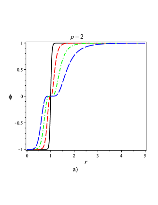
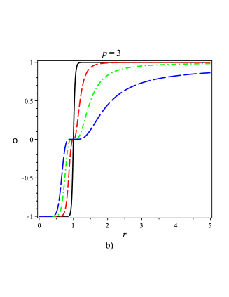
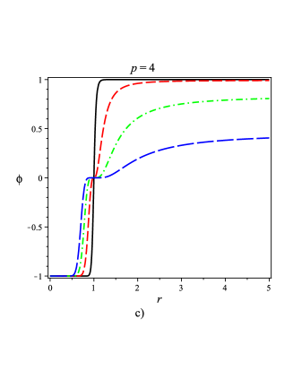
Figure 1: A one-field model for $p-$balls in $(D,1)$-dimensions: function $\phi(r)$. We fix $r_{0}=1$, $\lambda=30$. We have a) $p=2$, b) $p=3$ and c) $p=4$. Curves are for $q=1$ (black), 3 (red), 5 (green) and 7 (blue).

Fig. 1 shows plots of $\phi(r)$ for fixed $\lambda,r_{0}$ and several values of $q$ and $p$. The scalar field $\phi(r)$ interpolates between zero and $\phi_{c}$, with i) $\phi_{c}=1$ for either $q=1$ or $p=2$ and ii) $\phi_{c}=\tanh^{q}[\lambda/(q(p-2)r_{0}^{p-2})]$ for $q>1$ and $p\neq 2$. For $q\neq 1$ the larger is $p$, the lower is $\phi_{c}$. We note from the figure that the $\phi(r)$ configurations is now of two kinks connected at $r=r_{0}$ with a flat region around $r_{0}$ that grows with $q$. The internal kink runs from $r=0$ to $r=r_{0}$ and has a compacton character whereas the external kink goes from $r=r_{0}$ to $r\to\infty$ and is a semi-compacton. As $p$ increases we see that the internal kink (for $r<r_{0}$) has its thickness reduced whereas the external kink (for $r>r_{0}$) has its thickness increased.

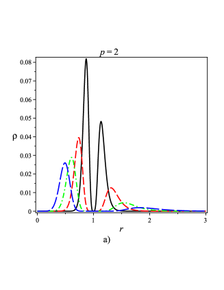
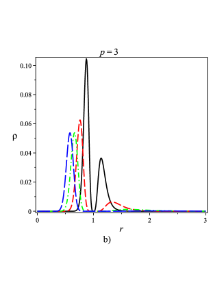
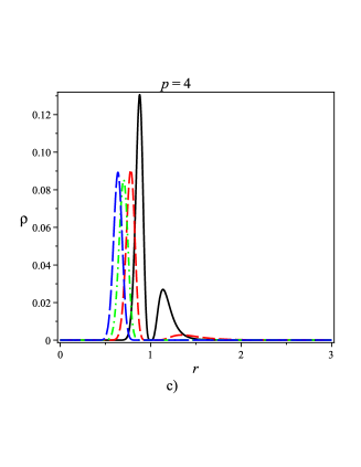
Figure 2: A one-field model for $p$-balls in $(D,1)$-dimensions: function $\rho(r)$. We fix $r_{0}=1$, $\lambda=30$. We have a) $p=2$, b) $p=3$ and c) $p=4$. Curves are for $q=3$ (black), 5 (red), 7 (green) and 9 (blue).

Fig. 2 shows plots of the radial energy density $\rho(r)$ for fixed $\lambda,r_{0}$ and several values of $q\geq 2$ and $p$. From the figures we see that the energy density is characterized by two peaks: a higher and thinner one, centered at $r<r_{0}$ and a lower and thicker one, centered at $r>r_{0}$. The distance between the peaks grows with $q$, enlarging the region around $r=r_{0}$ where $\rho\sim 0$, at the price of reducing the height of the peaks. For fixed $q$, the effect of the increasing of $p$ is an increasing of height and thinness of the peak at $r<r_{0}$ and a corresponding decreasing of the peak at $r>r_{0}$. The energy density for $q=1$ is characterized for a peak centered around $r=r_{0}$, and does not depend sensibly on $p$. Here we will consider the coupling $F(\phi)=\phi^{2}$, corresponding to the Schrödinger-like potential

$$V = \frac{\jmath(\jmath+p-2)}{r^{2}}+\eta\tanh^{2q}(\eta_{p}),\,p=2,3,....$$ (63)

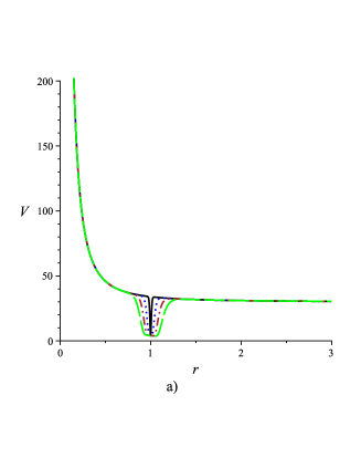
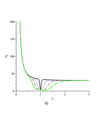
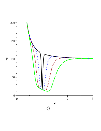
Figure 3: A one-field model for $p-$balls in $(D,1)$-dimensions: Schrödinger potentials $V$ for $\jmath=2$, $r_{0}=1$, $p=2$ and $q=1$ (black line), $q=3$ (blue dotted line), $q=5$ (brown dashdotted line), $q=7$ (green longdashed line). Plots are for a) $\eta=30$, $\lambda=100$, b) $\eta=30$, $\lambda=30$ and c) $\eta=100$, $\lambda=30$.

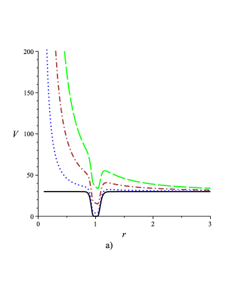
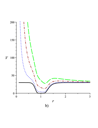
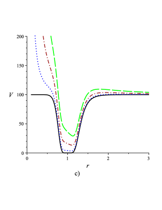
Figure 4: A one-field model for $p-$balls in $(D,1)$-dimensions: Schrödinger potentials $V$ for $r_{0}=1$, $p=2$, $q=5$ and $\jmath=0$ (black line), $\jmath=2$ (blue dotted line), $\jmath=4$ (brown dashdotted line), $\jmath=6$ (green longdashed line). Plots are for a) $\eta=30$, $\lambda=100$, b) $\eta=30$, $\lambda=30$ and c) $\eta=100$, $\lambda=30$.

	$q=1$		$q=3$		$q=5$		$q=7$		n
	$j=0$	$j=2$	$j=0$	$j=2$	$j=0$	$j=2$	$j=0$	$j=2$
$\eta=30,\;\lambda=100$	–	–	28.6227	–	24.8245	29.0266	20.5476	24.8500	1
$\eta=30,\;\lambda=30$	29.4788	–	19.5224	23.8051	11.4668	15.5708	7.1019	10.9721	1
	–	–	–	–	–	–	22.9866	27.0932	2
$\eta=100,\;\lambda=30$	90.8870	95.2469	41.9699	46.0534	20.1460	24.1420	11.2155	15.0803	1
	–	–	–	–	66.4764	70.7870	40.1402	44.4125	2
	–	–	–	–	99.3950	–	73.4681	77.6431	3
	–	–	–	–	–	–	95.9278	98.6800	4

Table 1: A one-field model for $p-$balls in $(D,1)$-dimensions: eigenvalues $M_{n\jmath}^{2}$, solutions of Eq. (43) for $\jmath=0$ and $\jmath=2$. We fix $r_{0}=1$, $p=2$, with $q$, $\lambda$ and $\eta$ of Schrödinger potentials for $\jmath=2$ corresponding to Figs. 3 and 4.

Fig. 3 shows some plots for $V(r)$ for fixed values of $p,r_{0},\jmath$ and several values of $q$, $\eta$ and $\lambda$. We note that the potentials are strictly positive, with $V(r\to 0)=\infty$ and a minimum around $r=r_{0}$. The structure of the potential shows that there are possibly bound states, to be investigated numerically. Comparing Figs. 3a-c we see that the increasing of $q$ or the decreasing of $\lambda$ enlarges the region around the local minimum, favoring the appearance of bound states. In addition, the increasing of $\eta$ turns the minimum deeper, also favoring bound states. This is confirmed with the eigenvalues obtained numerically, presented in Table I.

Fig. 4 shows some plots for $V(r)$ for fixed values of $p,r_{0},q$ and several values of $\lambda$, $\eta$ and $\lambda$. This figure shows that, for fixed parameters, an increasing in $\jmath$ decreases the possibility of occurrence of bound states. This is confirmed from the results of Tables I and II. The case $\jmath=0$ is special since there is no possibility of resonances. For larger values of $\jmath$, there is an increasing of a local maximum around $r=r_{0}$, increasing the possibility of occurrence of resonant states.

Fig. 5 shows $V(r)$ for fixed values of $\eta,\lambda,r_{0},\jmath$ and several values of $q$ and $p$. Comparing Figs. 5a-c we see that, for fixed parameters, the increasing of $p$ reduces the value of $V(r\to\infty)$. On the other hand this occurs simultaneously with the enlargement of the region around the local minimum (more evident for larger $q$). Concerning to the influence for the occurrence of bound states, the former character reduces the probability whereas the latter increases it. Then there is a competition between both effects. In particular Fig. 5c shows that for $q=7$ and $p=6$ the minimum of the potential disappears and there is no possibility of bound states. This signals that for large values of $q$ (i.e., $q\sim 7$), intermediate values of $p$ are better for obtaining more bound states. This analysis is confirmed from Table II, which shows that, for $q=5$ the occurrence of bound states is more frequent for $p=4$ and $p=5$ whereas for $q=7$ this occurs for $p=3$ and $p=4$.

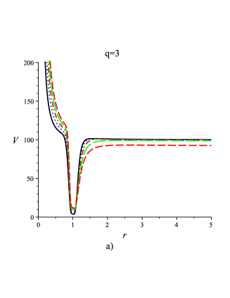
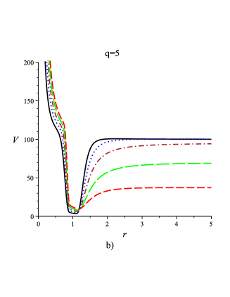
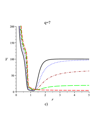
Figure 5: A one-field model for $p-$balls in $(D,1)$-dimensions: Schrödinger potentials $V$ for $\jmath=2$, $r_{0}=1$, $\eta=100$, $\lambda=30$ and $p=2$ (black line), $p=3$ (blue dotted line), $p=4$ (brown dashdotted line), $p=5$ (green longdashed line) and $p=6$ (red dashed line). Plots are for a) $q=3$, b) $q=5$ and c) $q=7$.

	$p=2$		$p=3$		$p=4$		$p=5$		$p=6$		$p=7$		$n$
	$j=0$	$j=2$	$j=0$	$j=2$	$j=0$	$j=2$	$j=0$	$j=2$	$j=0$	$j=2$	$j=0$	$j=2$
$q=3$	41.9699	46.0534	41.5186	47.4958	40.6852	48.4558	39.4634	48.9136	37.8409	48.8321	35.8017	48.1530	1
	–	–	99.779	–	97.8555	–	93.7645	–	87.0198	–	77.3044	–	2
$q=5$	20.1460	24.1420	19.3599	24.9835	17.9279	24.9191	15.8604	23.8675	13.1655	21.6049	9.8750	–	1
	66.4764	70.7870	62.7023	68.2819	55.8200	62.1088	45.5658	51.7269	31.8084	36.0979	–	–	2
	99.39.50	–	93.7420	97.2674	81.3528	85.2906	61.7843	65.0786	–	–	–	–	3
	–	–	–	–	91.2896	92.9968	67.7097	68.9111	–	–	–	–	4
$q=7$	11.2155	15.0803	10.2061	15.2934	8.4188	14.1784	5.9333	11.3420	2.9698	–	–	–	1
	40.1402	44.4125	35.3980	40.5926	26.9721	32.1424	15.0591	18.0844	–	–	–	–	2
	73.4681	77.6431	61.9651	66.2717	42.8930	46.5882	19.0888	–	–	–	–	–	3
	95.9278	98.6800	81.1822	84.3789	53.5926	56.0433	–	–	–	–	–	–	4
	–	–	91.9072	93.7907	60.0097	61.5195	–	–	–	–	–	–	5
	–	–	96.7928	97.4313	–	64.5802	–	–	–	–	–	–	6

Table 2: A one-field model for $p-$balls in $(D,1)$-dimensions: eigenvalues $M_{n\jmath}^{2}$, solutions of Eq. (43) for $\jmath=0$ and $\jmath=2$. We fix $r_{0}=1$, $\eta=100$, $\lambda=30$, with $p$ and $q$ of Schrödinger potentials for $\jmath=2$ corresponding to Fig. 5.

IV A two-field model

In this section we will consider the model

$$W(\phi,\chi)=\lambda\bigg{(}\phi-\frac{1}{3}\phi^{3}-s\phi\chi^{2}\bigg{)}.$$ (65)

With this choice of $W$, the potential $\tilde{V}(\phi,\chi)=(1/2)(W_{\phi}^{2}+W_{\chi}^{2})$ was introduced in Ref. BSR to construct Bloch walls. The limit $s\to 0.5$ turns the two-field problem into a one-field one, recovering the model of an Ising wall. This can be better seen in the explicit solutions $\phi(\xi)$ and $\chi(\xi)$ bellow. The equation of motion for the scalar fields, Eq. (14) is rewritten, after a change of variables $d\xi=1/r^{p-1}dr$, as

$$\frac{d\phi}{d\xi} = W_{\phi},$$ (66)

$$\frac{d\chi}{d\xi} = W_{\chi},$$ (67)

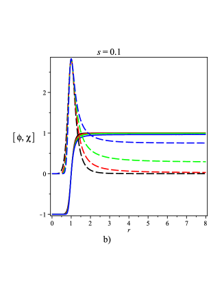
Figure 6: A two-field model for $p-$balls in $(D,1)$-dimensions: functions $\phi(r)$ (kink-like, solid lines) and $\chi(r)$ (lump-like, traced lines). We fix $r_{0}=1$, $\lambda=30$. We have a) $s=0.06$ and b) $s=0.1$. Curves are for $p=2$ (black), 3 (red), 4 (green) and 5 (blue).

with solution

$$\phi(\xi) = \tanh(2\lambda s\xi),$$ (68)

$$\chi(\xi) = \sqrt{\frac{1}{s}-2}\mathrm{sech}(2\lambda s\xi).$$ (69)

Back to $r$ variable, explicit expressions for the scalar field profiles and consequently for the energy density can be easily attained. We have, for $p\geq 2$,

$$\phi(r) = \tanh(\tau_{p}),$$ (70)

$$\chi(r) = \sqrt{\frac{1}{s}-2}\mathrm{sech}(\tau_{p}),$$ (71)

$$\rho(r) = \frac{\left(2\lambda s\right)^{2}}{r^{2p-2}}\mathrm{sech}^{4}(\tau_{p})\left\{1+\left(\frac{1}{s}-2\right)\mathrm{sinh}^{2}(\tau_{p})\right\}.$$

where

$$\tau_{p}=2\lambda s\xi(r)$$ (72)

and $\xi(r)$ given by Eq. (27), for $p=2$ and by Eq. (28), for p=3,4,….

Fig. 6 shows plots of $\phi(r)$ and $\chi(r)$ for fixed $\lambda,r_{0}$ and several values of $s$ and $p$. The scalar field $\phi(r)$ interpolates between $-1$ and $\phi_{c}$ , with $\phi_{c}=1$ for $p=2$ and $\phi_{c}=\tanh[2\lambda s/((p-2)r_{0}^{p-2})]$ for $p\neq 2$. The scalar field $\chi(r)$ interpolates between zero and $\chi_{c}$, with $\chi_{c}=0$ for $p=2$ and $\chi_{c}=\sqrt{(1/s)-2}\mathrm{sech}[2\lambda s/((p-2)r_{0}^{p-2})]$ for $p\neq 2$. Starting from $p=2$, the larger is $p$, the lower is $\phi_{c}$ and the larger is $\chi_{c}$. This means that with the increasing of $p$ the $\phi(r)$ and $\chi(r)$ configurations are, respectively, more departed from a usual kink and lump configurations in $r$, centered at $r=r_{0}$. Comparing Figs. 6a and 6b we see that, for all other parameters fixed, larger values of $s$ make the profiles of $\phi(r)$ almost indistinguishable from a thin kink-like defect centered at $r=r_{0}$. We have also verified that larger values of $\lambda$ turn the defect thinner and turn $\phi_{c}$ and $\chi_{c}$ closer to 1 and 0, recovering the kink and lump profiles for $\phi(r)$ and $\chi(r)$, respectively.

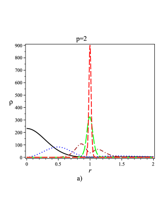
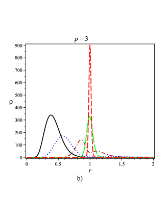
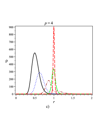
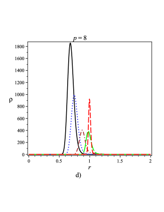
Figure 7: A two-field model for $p-$balls in $(D,1)$-dimensions: energy density $\rho(r)$ for $r_{0}=1$ and $\lambda=30$, $s=1/60$ (black line), $s=0.03$ (blue dotted line), $s=0.1$ (brown dash dotted line), $s=0.3$ (green longdash line), $s=0.5$ (red dashed line). Plots are for a) $p=2$, b) $p=3$, c) $p=4$ and d) $p=8$.

Fig. 7 shows plots of the energy density $\rho(r)$ for fixed $\lambda,r_{0}$ and several values of $s$ for $p=2,3,4$ and 8. From Fig. 7a we see that for $p=2$ the behavior of the energy density changes from a lump centered in $r=0$ $\left(s=\frac{1}{2\lambda}\right)$ to a high peak centered around $r_{0}$ $\left(s=0.5\right)$. Comparing Figs. 7a-d we see that the peaks for $s\simeq 0.5$ do not depend on the number $p$ of transverse dimensions. However, for lower values of $s$ the behavior of $\rho(r)$ changes sensibly. Indeed, for small $s$ the lump centered at $r=0$ occurs only for $p=2$. For $p\geq 3$ there appears a broad peak for centered at a $0<r<r_{0}$. The larger is $p$, the higher and thinner is this peak. For $p\geq 6$ the peak for small $s$ turns to be the higher in comparison to those occurring for larger values of $s$. Fig. 7d shows this effect for $p=8$. The influence of $\lambda$ on the energy density can be seen in Fig. 8 for $p=2$. Note that the increase of $\lambda$ turns the energy density more centered around $r=r_{0}$. At the same time this reduces the relative maximum of the energy density for lower values of $s$ in comparison to the higher ones. We noted a similar behavior with the variation of $\lambda$ for $p=3$.

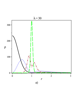
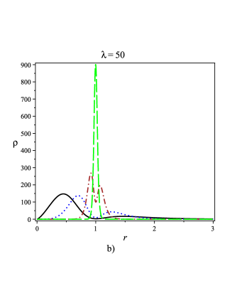
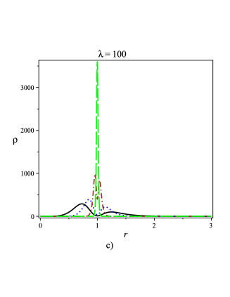
Figure 8: A two-field model for $2-$balls in $(D,1)$-dimensions: Energy density $\rho(r)$ for $r_{0}=1$, $p=2$ and $s=1/60$ (black line), $s=0.03$ (blue dotted line), $s=0.1$ (brown dash dotted line), $s=0.3$ (green longdash line). Plots are for a) $\lambda=30$, b) $\lambda=50$ and c) $\lambda=100$.

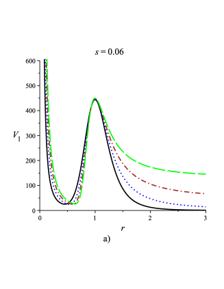
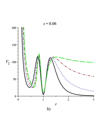
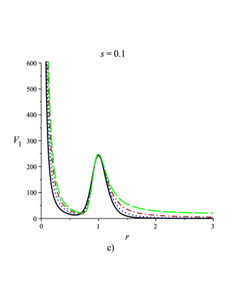
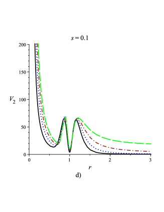
Figure 9: A two-field model for $p-$balls in $(D,1)$-dimensions: Schrödinger potentials $V_{1}(r)$ (left) and $V_{2}(r)$ (right) for $\jmath=2$, $r_{0}=1$, $\eta=30$, $\lambda=30$ and $p=2$ (black line), $p=3$ (blue dotted line), $p=4$ (brown dash dotted line), $p=5$ (green longdash line). Plots are for $s=0.06$ and $s=0.1$.

$V$

$s$

$p=2$

$p=3$

$p=4$

$p=5$

$p=6$

$p=7$

$n$

$j=0$

$j=2$

$j=0$

$j=2$

$j=0$

$j=2$

$j=0$

$j=2$

$j=0$

$j=2$

$j=0$

$j=2$

$V_{1}$

$0.06$

–

–

–

–

18.4988

–

16.9502

65.5898

15.9269

68.9682

15.1955

72.4943

1

–

–

–

–

–

–

66.3794

–

62.7636

149.3757

60.0992

153.8414

2

–

–

–

–

–

–

–

–

137.6105

–

132.5581

254.5088

3

–

–

–

–

–

–

–

–

–

–

228.5419

–

4

$V_{1}$

$0.10$

–

–

–

–

–

–

13.3597

–

12.9701

–

12.6690

61.0235

1

–

–

–

–

–

–

–

–

–

–

50.0838

–

2

$V_{2}$

$0.06$

–

–

–

–

17.6796

–

16.0810

57.2498

14.9927

58.2993

14.1899

59.1008

1

–

–

–

–

–

–

51.6688

71.1128

49.2798

73.4513

47.0188

75.5898

2

–

–

–

–

–

–

68.0193

–

65.5464

–

63.4274

–

3

–

–

–

–

–

–

–

–

108.7936

–

100.9167

–

4

$V_{2}$

$0.10$

–

–

–

–

–

–

11.9547

–

11.4910

–

11.1174

48.1639

1

–

–

–

–

–

–

–

–

–

–

38.0263

–

2

Table 3: A two-field model for $p-$balls in $(D,1)$-dimensions: eigenvalues $M_{n\jmath}^{2}$, solutions of Eq. (43) for $\jmath=0$ and $\jmath=2$. We fix $r_{0}=1$, $\eta=30$, $\lambda=30$, with Schrödinger potentials for $\jmath=2$ corresponding to Fig. 9.

In the following we will consider separately the couplings $F_{1}(\chi)=\chi^{2}$ and $F_{2}(\phi,\chi)=(\phi\chi)^{2}$. The corresponding Schrödinger-like potentials are

$$V_{1} = \frac{\jmath(\jmath+p-2)}{r^{2}}+\eta\bigg{(}\frac{1}{s}-2\bigg{)}\mathrm{sech}^{2}(\tau_{p}),\,p=2,3,...$$ (73)

$$V_{2} = \frac{\jmath(\jmath+p-2)}{r^{2}}+\eta\bigg{(}\frac{1}{s}-2\bigg{)}\tanh^{2}(\tau_{p})\mathrm{sech}^{2}(\tau_{p}),\,p=2,3,....$$ (74)

Fig. 9 shows some plots for $V_{1}(r)$ and $V_{2}(r)$ for fixed values of $\eta,\lambda,r_{0},\jmath$ and several values of $p$. For all values of $p$ the potentials are strictly positive. Also, for $p=2$ we have $V_{1}(r\to\infty)=0$ and $V_{2}(r\to\infty)=0$, showing that bound states are absent. For $p\geq 3$ we have $V_{1}(r\to\infty)=\eta F_{1}(\phi_{c},\chi_{c})\neq 0$ and $V_{2}(r\to\infty)=\eta F_{2}(\phi_{c},\chi_{c})\neq 0$ and one can investigate the existence of bound states.

First of all we consider the case $\jmath=2$. For the potentials shown in Fig. 9, and also for higher values of $p$, the existence of bound states was investigated and some results could be found according to Table III. For $s=0.06$ and $s=0.1$ we could not find bound states for neither $V_{1}$ nor $V_{2}$ when $p=2,3,4$. Bound states start to appear for $p\geq 5$ for $s=0.06$ and $p\geq 7$ for $s=0.1$. The results show that lower values of $s$ are better for the occurrence of bound states. As explained above, $s\to 0.5$ recover a one-field $\phi$ model. Then, the presence of a second scalar field $\chi$ contributes to trapping spin-0 particles. In other words, $p-$balls with more internal structure are more able to trap scalar particles. Also, for fixed $s$ and larger number $p$ of transverse dimensions, bound states occur with larger masses for potential $V_{1}$ than for potential $V_{2}$. This shows that, for a trapping mechanism, the quadratic coupling $\chi^{2}$ is better that the quartic one $\phi^{2}\chi^{2}$. Moreover, a multidimensional $p-$ball with larger $p$ is a better trapping mechanism, as $V_{1}(r\to\infty)$ and $V_{2}(r\to\infty)$ grows with $p$. This is confirmed in Table III. Indeed, the larger is $p$, the greater is the number of bound states. Also, the asymptotic values $V_{1}(r\to\infty)$ and $V_{2}(r\to\infty)$ grow with $\lambda$ and $\eta$. This signals that in order to grow the probability for the occurrence of bound states one must have $\eta,\lambda\gg 1$ and decrease the ratio $\lambda/\eta$. This can be seen in Fig. 10 where $\lambda/\eta=3/10$ (compare with Fig. 9 where $\lambda/\eta=1$). Corresponding eigenvalues are described in Table IV. From the results for $\lambda=30$ we see that for $\lambda/\eta=3/10$ and $s=0.06$ there occur bound states for $p\geq 4$ (compare with the results of Table III for $\lambda/\eta=1$ where bound states appear for $p\geq 4$).

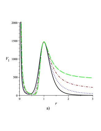
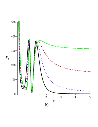
Figure 10: A two-field model for $p-$balls in $(D,1)$-dimensions: Schrödinger potentials a) $V_{1}(r)$ (left) and b) $V_{2}(r)$ (right) for $\jmath=2$, $r_{0}=1$, $\eta=100$, $\lambda=30$, $s=0.06$ and $p=2$ (black line), $p=3$ (blue dotted line), $p=4$ (brown dash dotted line), $p=5$ (green longdash line).

$V$	$p=2$		$p=3$		$p=4$		$p=5$		$p=6$		$p=7$		$n$
	$j=0$	$j=2$	$j=0$	$j=2$	$j=0$	$j=2$	$j=0$	$j=2$	$j=0$	$j=2$	$j=0$	$j=2$
$V_{1}$	–	–	–	–	21.5827	72.5884	19.3059	74.4329	17.8608	77.1262	16.8559	80.2321	1
	–	–	–	–	84.3439	166.9563	76.1917	166.9618	70.8185	168.9305	67.0053	171.9820	2
	–	–	–	–	–	–	167.7651	285.8629	157.0522	286.6631	149.2038	289.1227	3
	–	–	–	–	–	–	289.9211	427.9080	273.7365	427.8130	261.4261	429.7415	4
	–	–	–	–	–	–	438.2871	–	417.4132	589.5117	400.9835	591.3007	5
	–	–	–	–	–	–	–	–	584.4205	–	564.7141	770.9510	6
	–	–	–	–	–	–	–	–	–	–	749.3110	–	7
$V_{2}$	–	–	–	–	21.3410	71.6610	19.0653	73.3757	17.6114	75.8862	16.5924	78.7597	1
	–	–	–	–	82.9807	127.0889	74.9047	127.4501	69.5199	127.3683	65.6502	126.8865	2
	–	–	–	–	119.3195	–	117.8118	163.8790	115.8253	165.8453	113.3861	168.7750	3
	–	–	–	–	–	–	164.1016	273.4499	153.9482	272.8946	146.5262	270.4678	4
	–	–	–	–	–	–	273.8062	310.4326	259.9589	300.8025	248.3106	290.6058	5
	–	–	–	–	–	–	304.4750	–	290.8448	–	275.0988	339.6651	6
	–	–	–	–	–	–	–	–	359.1479	–	332.6537	–	7
	–	–	–	–	–	–	–	–	–	–	345.4081	–	8

Table 4: A two-field model for $p-$balls in $(D,1)$-dimensions: eigenvalues $M_{n\jmath}^{2}$, solutions of Eq. (43) for $\jmath=0$ and $\jmath=2$. We fix $r_{0}=1$, $\eta=100$, $\lambda=30$, $s=0.06$, with Schrödinger potentials for $\jmath=2$ corresponding to Fig. 10.

Now note that the potentials for coupling $F_{1}$ are characterized by a local maximum at $r=r_{0}$ whereas for $F_{2}$ there is a local minimum at $r=r_{0}$ surrounded by two local maxima. The higher local peak for $V_{1}$ in comparison to the two local ones for $V_{2}$ suggests that, with the same set of parameters, resonant states are most probable with quadratic coupling $F_{1}$ than with quartic coupling $F_{2}$. This is in accord to the behavior of couplings concerning to the occurrence of bound states. We also see that the height of the local maxima grows with the decreasing of $s$, favoring the appearance of resonances. Then we expect the presence of a second scalar field $\chi$ to be important for the increasing in the number and lifetime of resonances. We also found that for all other parameters fixed, the best choice for reducing the asymptotical value of $V_{1}$ and simultaneously increasing the difference between the local maxima and minima is to keep $\eta,\lambda\gg 1$ and increase the ratio $\lambda/\eta$. This can be seen in Fig. 11, for $\lambda/\eta=10/3$ (compare with Fig. 9, where $\lambda/\eta=1$ and with Fig. 10, where $\lambda/\eta=3/10$). However, this occurs at the price of making the barrier thinner. Then we expect that an increasing of $\lambda/\eta$ increases the chances for getting a larger number of resonances, but with lower lifetimes.

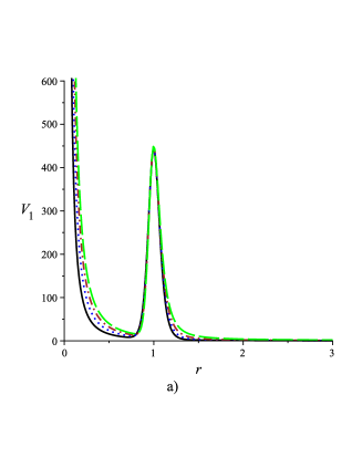
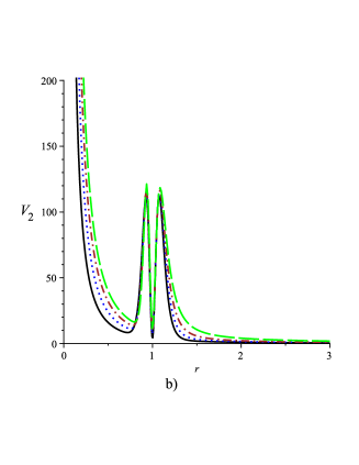
Figure 11: A two-field model for $p-$balls in $(D,1)$-dimensions: Schrödinger potentials a) $V_{1}(r)$ (left) and b) $V_{2}(r)$ (right) for $\jmath=2$, $r_{0}=1$, $\eta=30$, $\lambda=100$, $s=0.06$ and $p=2$ (black line), $p=3$ (blue dotted line), $p=4$ (brown dash dotted line), $p=5$ (green longdash line).

The influence of the variation of the angular momentum $\jmath$ can be seen in Fig. 12, where we present some plots for the potential $V_{1}$. The potentials for $\jmath\geq 1$ are characterized by a local minimum and local maximum whose separation decreases with $\jmath$. This signals that the increasing of $\jmath$ reduces the possibility of occurrence of bound and resonant states. Case $\jmath=0$ is special since we have $V_{1}=0$ at $r=0$, being the case with highest possibility for occurrence of such states. Concerning to bound states this is confirmed from the results of Tables III and IV, where one can compare cases $\jmath=0$ and $\jmath=2$. Then former analysis and conclusions of the Schrödinger potential and bound states made for $\jmath=2$ also apply for general values of $\jmath$. Similar analysis for potential $V_{2}$ leads to the same conclusion: lower values of $\jmath$ are favored for occurrence of bound and resonant states.

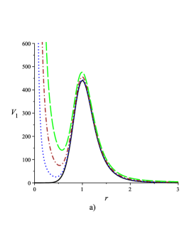
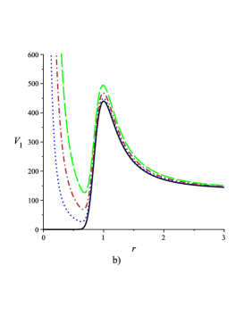
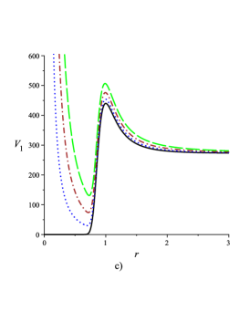
Figure 12: A two-field model for $p-$balls in $(D,1)$-dimensions: Schrödinger potentials $V_{1}(r)$ for a) $p=2$, b) $p=5$, c) $p=7$ and $r_{0}=1$, $\eta=30$, $\lambda=30$, $s=0.06$, $\jmath=0$ (black line), $\jmath=2$ (blue dotted line), $\jmath=4$ (brown dash dotted line), $\jmath=6$ (green longdash line).

Now we will consider specifically the effect of the number of longitudinal and transverse dimensions on the resonance effect. For the couplings $F_{1}$ and $F_{2}$, $\lambda s\geq 1/2$ and $\jmath\geq 1$ the potentials $V_{sch}$ for $r\ll r_{0}$ are dominated by the contributions of the angular momentum proportional to $1/r^{2}$,

$$V(r)\approx\frac{\jmath(\jmath+p-2)}{r^{2}},$$ (75)

and the nonsingular solutions in $r=0$ are given by Eq. (57), used for calculating the relative probability $P$.

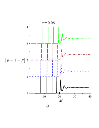
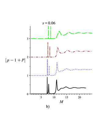
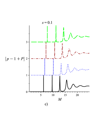
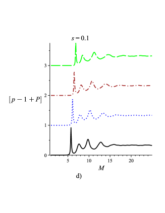
Figure 13: A two-field model for $p-$balls in $(D,1)$-dimensions: $(p-1)+P$ as a function of $M$ for coupling $F_{1}(\chi)$ (left) and $F_{2}(\phi,\chi)$ (right) for $\jmath=2$, $r_{0}=1$, $\eta=30$, $\lambda=30$, and $p=2$ (black line), $p=3$ (blue dotted line), $p=4$ (brown dash dotted line), $p=5$ (green longdash line). The plots are for $s=0.06$ and $s=0.1$, and correspond to potentials of Fig. 9.

Fig. 13 depicts $P$ (rescaled for ease comparison) as a function of $M_{n\jmath}\equiv M$ for several values of $p$ and $s$, corresponding to the Schrodinger-like potentials of Fig. 9. The plots show several peaks of resonances, followed by a plateau for larger masses where $P=r_{0}/r_{max}$. From the figure we note that lower masses correspond to thinner peaks, or longer-lived resonances. The low-mass resonances are more difficult to be obtained numerically, due to the requirement of a larger number of digits of precision. Comparing Figs. 13a and 13c or Figs. 13b and 13d we see that lower values of $s$ correspond to a larger number of resonance peaks. In addition, the peak separation is reduced for lower values of $s$. This shows that small values of $s$ are more effective for attaining resonances. The effect of the increasing in the number of extra dimensions $p$ is a displacement of the peak positions for larger masses, keeping the mass separation between the peaks almost unaltered. Figs. 13b and 13d shows the resonance peaks for coupling $F_{2}(\phi,\chi)$. Comparing this with Figs. 13a and 13c (related to $F_{1}(\chi)$), we see that for coupling $F_{2}(\phi,\chi)$ the number and masses of resonances is strongly reduced in comparison to the case of coupling $F_{1}(\chi)$. Indeed, even for $s=0.06$, Fig. 13b shows a pair of neighbor peaks, with only one with relative probability close to one. The sequence of almost equally spaced peaks present for coupling $F_{1}(\chi)$ (corresponding to Fig. 13a) is now absent. This shows that coupling $F_{2}(\phi,\chi)$ is less effective for the occurrence of resonances.

Fig. 14 shows some resonance peaks corresponding to $\eta=30$ and $\lambda=100$. Comparing with Figs 13, we note that the resonances observed are more easy to be numerically obtained, but also thicker, meaning lower lifetimes. This is in accord with the analysis of the influence of the ratio $\lambda/\eta$ for the Schrodinger-like potentials.

Concerning to the angular sector of the decomposition of the weak scalar field, the number of extra dimensions is the key point. In the remaining of this section we will consider separately some specific choices of the number $D$ of spatial dimensions up to $D=5$. The procedure for larger values of $D$ is straightforward.

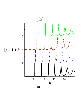
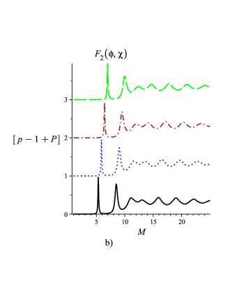
Figure 14: A two-field model for $p-$balls in $(D,1)$-dimensions: $(p-1)+P$ as a function of $m$ for coupling $F_{1}(\chi)$ (left) and $F_{2}(\phi,\chi)$ (right) for $\jmath=2$, $r_{0}=1$, $\eta=30$, $\lambda=100$, $s=0.06$ and $p=2$ (black line), $p=3$ (blue dotted line), $p=4$ (brown dash dotted line), $p=5$ (green longdash line). The plots correspond to potentials of Fig. 11.

IV.1 $p-$balls in $(3,1)$-dimensions

The simplest choice is to consider $p-$balls in $(3,1)$-dimensions. In this case the only possibility is to construct a radial defect with $p=2$ spatial dimensions. This is a tube-like defect and has already been studied by us in Refs. cgms1 ; cgms2 . Requiring $\rho(r)$ finite in $r=0$ restricts the parameters to satisfy $\lambda s\geq 1/2$ when $\lambda>1$. For large values of $\lambda$, there exists a value $s_{0}$ so that for $\frac{1}{2\lambda}<s<s_{0}$, the effect of the field $\chi$ is stronger and the defect appears as a thick tube structure whose center is localized between the origin and $r_{0}$. The decomposition of the weak scalar field $\Phi(t,x^{1},x^{2})$ is

$$\Phi(t,x^{1},r,\varphi)=\sum_{n\ell}\xi_{n\ell}(t,x^{1})\varsigma_{n,\ell}(r)Y_{\jmath}(\varphi),$$ (76)

where the spherical harmonic is $Y_{\ell}(\varphi)=e^{i\ell\varphi}$ and $\varsigma_{n,\ell}(r)$ satisfies a $(2,1)$-dimensional Klein-Gordon equation.

IV.2 $p-$balls in $(4,1)$-dimensions

In this case we have two possibilities: i) to construct a radial defect with $p=2$ spatial transverse dimensions and $(2,1)$ longitudinal dimensions, or ii) to construct a radial defect with $p=3$ spatial transverse dimensions and $(1,1)$ longitudinal dimensions. In the following we will consider these two possibilities separately.

IV.2.1 $p-$balls in $(4,1)$-dimensions with $p=2$ transverse dimensions

The defect is characterized by a potential which generates, respectively, kink-like and lump-like solutions for the scalar fields $\phi(r)$ and $\chi(r)$, as well as energy density $T_{00}(r)$ with the same profile found for the case analyzed in Sect. IV.1 for $(3,1)-$dimensions. This is expected since we have the same number (two) of transverse dimensions. All would follow the same as in Sec. IV.1: the decomposition of the spherical harmonics $Y_{\ell}$, Schrödinger-like potentials $V_{sch}$ and relative probabilities $P$. The difference is that in the present case of $(4,1)-$dimensions we have $(2,1)$ longitudinal dimensions. This is reflected in the longitudinal part $\xi_{n\ell}$ of the decomposition of the weak scalar field $\Phi(t,x^{1},x^{2})$,

$$\Phi(t,x^{1},x^{2},r,\varphi)=\sum_{n\ell}\xi_{n\ell}(t,x^{1},x^{2})\varsigma_{n,\ell}(r)Y_{\ell}(\varphi),$$ (77)

which now satisfy a $(2,1)$-dimensional Klein-Gordon equation.

IV.2.2 $p-$balls in $(4,1)$-dimensions with $p=3$ transverse dimensions

The defect is a 3-dimensional sphere. For larger values of $\lambda$ and $s$, the defects looks like as a thin ball centered around $r_{0}$ and the field $\phi$ has stronger contribution to the energy density. On the other hand, when we have larger values of $\lambda$ and lower values of $s$ are formed peaks between origin and $r_{0}$, which results in higher contribution of the $\chi$ field and the defect has a thicker structure. The spherical harmonic is $Y_{\ell}(\varphi,\theta)=\sum_{-\ell}^{\ell}Y_{\ell m}(\varphi,\theta)$.

IV.3 $p-$balls in $(5,1)$-dimensions

In this case we have three possibilities: i) to construct a radial defect with $p=2$ spatial transverse dimensions and $(3,1)$ longitudinal dimensions. The procedure for the transverse dimensions is analogous to Sec. IV.1, with the exception that now the longitudinal part $\xi_{n\ell}$ of the decomposition of the weak scalar field $\Phi$ satisfy a $(3,1)-$dimensional Klein-Gordon equation. ii) to construct a radial defect with $p=3$ spatial transverse dimensions and $(2,1)$ longitudinal dimensions. The results for the transverse dimensions is analogous to Sec. IV.2.2, with the exception that now the longitudinal part $\xi_{n\ell}$ of the decomposition of the weak scalar field $\Phi$ satisfy a $(2,1)-$dimensional Klein-Gordon equation. iii) to construct a radial defect with $p=4$ spatial transverse dimensions and $(1,1)$ longitudinal dimensions.

V A three-field model

In this section we will consider some three-field models. The numerical analysis of bound and resonant states follows the same prescription done in the two previous sections and we will not pursue in this direction here, focusing mainly in the analysis of the Schrödinger-like potentials. We start with a simple extension of the previous model, given by blw

$$W(\phi,\chi,\sigma)=\lambda\bigg{(}\phi-\frac{1}{3}\phi^{3}-s\phi(\chi^{2}+\sigma^{2})\bigg{)},$$ (78)

where $s$ is a real parameter. The equation of motion for the scalar fields, Eq. (14) is rewritten, after a change of variables $d\xi=1/r^{p-1}dr$, as

$$\frac{d\phi}{d\xi} = W_{\phi},$$ (79)

$$\frac{d\chi}{d\xi} = W_{\chi},$$ (80)

$$\frac{d\sigma}{d\xi} = W_{\sigma}.$$ (81)

One solution connecting the minima $(\pm 1,0,0)$ of the potential is blw

$$\phi(\xi) = \tanh(2\lambda s\xi),$$ (82)

$$\chi(\xi) = \sqrt{\frac{1}{s}-2}\cos(\vartheta)\mathrm{sech}(2\lambda s\xi),$$ (83)

$$\sigma(\xi) = \sqrt{\frac{1}{s}-2}\sin(\vartheta)\mathrm{sech}(2\lambda s\xi).$$ (84)

with $0\leq s\leq 0.5$ and $0\leq\vartheta<2\pi$, where now $\vartheta$ is a new parameter of the model. Back to $r$ variable, explicit expressions for the scalar field profiles and consequently for the energy density can be easily attained. We have, for $p\geq 2$,

$$\phi(r) = \tanh(\tau_{p}),$$ (85)

$$\chi(r) = \sqrt{\frac{1}{s}-2}\cos(\vartheta)\mathrm{sech}(\tau_{p}),$$ (86)

$$\sigma(r) = \sqrt{\frac{1}{s}-2}\sin(\vartheta)\mathrm{sech}(\tau_{p}),$$ (87)

$$\rho(r) = \frac{\left(2\lambda s\right)^{2}}{r^{2p-2}}\mathrm{sech}^{4}(\tau_{p})\left\{1+\left(\frac{1}{s}-2\right)\mathrm{sinh}^{2}(\tau_{p})\right\}.$$

with $\tau_{p}$ given by Eq. (72). One can interpret the $\phi$ field as forming a host hypersphere, with the fields $\chi$ and $\sigma$ giving its internal structure. The balancing of the internal fields is given by the parameter $s$. We can also consider the real scalar fields $\chi$ and $\sigma$ as the real and imaginary part of a complex scalar field $\zeta$, with the model given by

$$W(\phi,\zeta)=\lambda\bigg{(}\phi-\frac{1}{3}\phi^{3}-s\phi|\zeta|^{2}\bigg{)}.$$ (88)

A simple coupling is $F_{3}=|\zeta|^{2}=(\chi^{2}+\sigma^{2})$. The explicit solutions $\chi(r),\sigma(r)$ shows that this coupling recovers the results obtained for $F_{1}(\chi)$ from Sect. IV. Another coupling is $F_{4}=a\phi^{2}+b_{1}\chi^{2}+b_{2}\sigma^{2}$, with $a,b_{1},b_{2}>0$. Cases $a=b_{2}=0,b_{1}=1$ or $a=0,b_{1}=b_{2}=1$ recover coupling $F_{1}$. For coupling $F_{4}$, the Schrödinger-like potential is

$$V_{4}=\frac{\jmath(\jmath+p-2)}{r^{2}}+\eta a\tanh^{2}(\tau_{p})+\eta b\bigg{(}\frac{1}{s}-2\bigg{)}\mathrm{sech}^{2}(\tau_{p}),\,p=2,3,...,$$ (89)

with $b=b_{1}\cos^{2}(\vartheta)+b_{2}\sin^{2}(\vartheta)$.

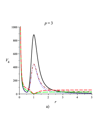
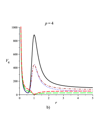
Figure 15: Schrödinger potential $V_{4}$ for $\jmath=2$, $r_{0}=1$, $\eta=30$, $\lambda=30$, $s=0.06$ and $a=0,b=2$ (black line), $a=0,b=1$ (blue dotted line), $a=1,b=1$ (brown dash dotted line), $a=1,b=0$ (green longdash line), $a=2,b=0$ (red dashed line). Plots are for $p=3$ (left) and $p=4$ (right).

Figure 15 shows potential $V_{4}$ for $p=3$, $p=4$ and several values of parameters $a,b$. From the figure we see that a parameter $b\neq 0,a=0$ results in a local maximum around $r=r_{0}$ that increases with $b$. With $b\neq 0$, a value $a\neq 0$ contributes to a small enlargement of the peak of $V_{4}$ around $r=r_{0}$. For $b=0,a\neq 0$ the local maximum disappears and only bound states are possible. The analysis shows that a parameter $b\neq 0$ (meaning a quadratic coupling with fields $\chi$ or $\sigma$) is crucial for the occurrence of resonances. Also a quadratic coupling with field $\phi$ is of secondary importance, when compared with the effect of similar couplings with the other two fields that form the defect. A quadratic coupling with only the $\phi$ field has no effect concerning to resonances. This illustrates the importance of the secondary fields $\chi,\sigma$ that give to the defect an internal structure. Comparing Figs. 15a and 15b we see that for $p=3$ we have more possibility for resonant states in comparison to $p=4$. The increasing of $V_{4}(r\to\infty)$ with $p$ shows that an intermediate value of $p$ is better for attaining bound states, in a similar conclusion achieved in Sect. III for one-field models. For $p=2$ the potential $V_{4}$ is a monotonically decreasing function, and there is neither bound nor resonant states.

Other couplings can be considered, but to further illustrate the generality of the construction of $p$-balls, here we choose to consider another model, restricted to a $Z_{2}\times Z_{2}$ symmetry in the $\chi$ and $\sigma$ axis blw :

$$W(\phi,\chi,\sigma)=\lambda\bigg{(}\phi-\frac{1}{3}\phi^{3}-s\phi(\chi^{2}+\sigma^{2})+rg\sigma^{2}\bigg{)}.$$ (90)

For $s>0$ and $-1<g<1$ the corresponding potential $V(\phi,\chi,\sigma)$ has six minima given by (in units of $\xi$)

$$v_{1,2} = (\pm 1,0,0),$$ (91)

$$v_{3,4} = \biggl{(}0,\pm\sqrt{\frac{1}{s}},0\biggr{)},$$ (92)

$$v_{5,6} = \biggl{(}g,0,\mp\sqrt{\frac{1}{s}(1-g^{2})}\biggr{)}.$$ (93)

For $s\neq 0$ the only solution connecting the minima $v_{1,2}$ is the one-field limit given by $\chi=\sigma=0$ and $\phi(\xi)=\tanh(\xi)$. Nontrivial solutions for the three scalar fields can be obtained connecting minima $v_{3,4}$ to $v_{5,6}$ and are given, with $sg^{2}=1$, by blw

$$\phi(\xi) = \frac{g}{2}(1+\tanh(\xi/g)),$$ (94)

$$\chi(\xi) = \pm\frac{1}{2}\sqrt{\frac{1}{s}}(1-\tanh(\xi/g)),$$ (95)

$$\sigma(\xi) = \pm\frac{1}{2}\sqrt{\frac{1}{s}(1-g^{2})}(1+\tanh(\xi/g)).$$ (96)

Back to $r$ variable, and for $p\geq 2$, we can obtain the following expressions for the scalar fields:

$$\phi(r) = \frac{g}{2}(1+\tanh(\xi(r)/g)),$$ (97)

$$\chi(r) = \pm\frac{1}{2}\sqrt{\frac{1}{s}}(1-\tanh(\xi(r)/g)),$$ (98)

$$\sigma(r) = \pm\frac{1}{2}\sqrt{\frac{1}{s}(1-g^{2})}(1+\tanh(\xi(r)/g)),$$ (99)

with $\xi(r)$ given by Eq. (27), for $p=2$ or (28), for $p=2,3,....$

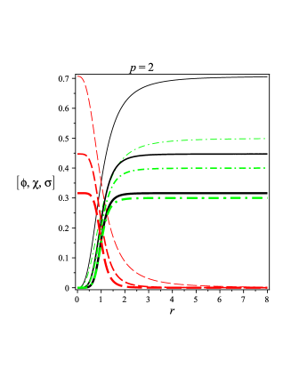
Figure 16: $2-$balls in $(D,1)$-dimensions for three scalar fields: functions $\phi(r)$ (black solid lines), $\chi(r)$ (red traced lines) and $\sigma(r)$ (green dashdotted lines). We fix $r_{0}=1$ and $\lambda=30$ and couplings $sg^{2}=1$. We have $s=1.01$ (thinner lines), $s=5$ and $s=10$ (thicker lines).

Figure 16 shows plots of $\phi(r)$, $\chi(r)$ and $\sigma(r)$ for $p=2$ and fixed $\lambda,r_{0}$ and several values of $s$. From the figure we see that all the three fields have a kink-like structure around $r=r_{0}$. Note that an increasing in $s$ (and correspondingly a decreasing in $g$) results in a thinner defect. The same effect occurs with the increasing of $p$, as can be seen from Fig. 17.

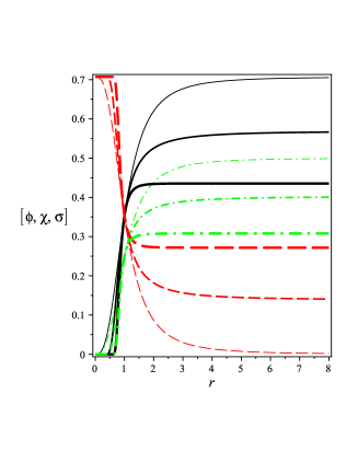
Figure 17: $p-$balls in $(D,1)$-dimensions for three scalar fields: functions $\phi(r)$ (black solid lines), $\chi(r)$ (red traced lines) and $\sigma(r)$ (green dashdotted lines). We fix $r_{0}=1$ and $\lambda=30$, $s=2$ and $sg^{2}=1$. We have $p=2$ (thinner lines), $p=4$ and $p=8$ (thicker lines).

For coupling $F_{5}=a\phi^{2}+b_{1}\chi^{2}+b_{2}\sigma^{2}$, with $a,b_{1},b_{2}>0$, the Schrödinger-like potential is

$$V_{5} = \frac{\jmath(\jmath+p-2)}{r^{2}}+\eta a\frac{g^{2}}{4}(1+\tanh(\xi(r)/g))^{2}$$ (100)

$$+\eta b\frac{1}{4}{\frac{1}{s}}(1-\tanh(\xi(r)/g))^{2}+\eta c\frac{1}{4}{\frac{1}{s}(1-g^{2})}(1+\tanh(\xi(r)/g))^{2},\,p=2,3,...,$$

which can also be investigated for possible occurrence of bound and resonant states.

VI Remarks and conclusions

In this work we introduced p-balls as topological defects in $(D,1)$ dimensions constructed with $\mathcal{M}\geq 1$ scalar fields which depend radially on only $2\leq p\leq D-2$ spatial dimensions. Such defects are characterized by an action that breaks translational invariance and are inspired on the physics of a brane with $D-p$ extra dimensions and $p$ transverse spatial dimensions. After presenting the general formalism, we have found BPS solutions living in the $p$ transversal dimensions and proved their stability. In order to analyze the localization of a scalar field $\Phi$ (named a weak field because we can neglect backreaction effects) in $D-p+1$-dimensions, we have considered a general coupling between the weak field and the scalars fields generating the topological defect. Our results have shown the existence of bound and/or resonant states which were addressed after a convenient decomposition of the weak scalar field in $D-p+1$ -dimensional spin-$0$ modes and its respective amplitudes in the transverse $p$-dimensions. As usual the spin-$0$ modes satisfy a $D-p+1$ dimensional Klein-Gordon equation whereas the amplitudes are decomposed in an angular part in terms of the generalized spherical harmonics and a radial part satisfying a Schrödinger-like equation.

We have particularized our analysis to the class of models where the $p-$balls are formed with one, two and three scalar fields. For the class of one-field models we have considered a region of parameters where a larger number of bound states are formed. It is characterized for $p-$balls with larger internal structure (large $q$), intermediate number of extra dimensions $3<p<5$, lower energy (lower coupling $\lambda$) and higher coupling parameter $\eta$. The two-field models resemble the Bloch brane model where we have considered two type of couplings. A quadratic coupling $\chi^{2}$ is better than the quartic one $\phi^{2}\chi^{2}$ concerning to the occurrence of either bound or resonant states. We have verified the presence of the second scalar field $\chi$ contributes to the increasing of trapping spin-$0$ particles. In these two-field models, the larger is $p$, the greater is the number of bound states, but the number of resonances is roughly the same. We have also explored some three-field models, finding from the analysis of the Schrodinger-like potential that in some cases an intermediate value of $p$ is better for the occurrence of bound states.

Concerning to the influence of $\jmath$, the probability of occurrence of bound states with $\jmath=0$ is higher in comparison to states with larger values of $\jmath$. This was verified numerically. On the other hand, for resonances the analysis of the Schrödinger potential shows that the behavior depends on the model. In our one-field model there is no such possibility for $\jmath=0$ whereas the possibility of occurrence of such states is low but grows with the increasing of $\jmath$. On the other hand for our two-field model the number of resonant states seems to accompany the tendency of bound states, with a decreasing in number with $\jmath$.

It is worthwhile to observe that we where able to establish a connection between the number of extra dimensions and the capability of trapping massive states. Such a study was attained by analyzing qualitatively the Schrodinger-like potentials and by performing numerical analysis. For all class of models considered, we could identify that initially there is an increasing of the number of bound states with $p$. For the one-field model this occurs up to a certain number of transverse dimensions; in this way there is an optimal number of transverse dimensions for trapping states. On the other hand, for the two-field model considered, we have investigated up to $p=7$ and the number of bound states always grow with $p$, whereas the number of resonances seems to be independent of $p$. Also we have confirmed that, for fixed $p$, the growing of the internal structure of the defect (connected with larger values of $q$ for the one-field model and smaller values of $s$ in the two-field and three-field models) lead to an increasing of the number of bound and/or resonance states.

Whether our results represent a general characteristic of the $p$-balls or the main conclusions are results of the particularities of the models here described deserves to be better understood. Advances in this direction will be reported elsewhere.

- (1) A. Vilenkin. Cosmic strings and other topological defects. Cambridge, 1994.
- (2) N. Manton, P. Sutcliffe. Topological Solitons. Cambridge, 2004.
- (3) J. Greensite, Prog. Part. Nucl. Phys. 51 (2003) 1; T. Suzuki, Nucl. Phys. Proc. Suppl. 30 (1993) 176; M. N. Chernodub,M. I. Polikarpov, in Confinement, Duality, and Nonperturbative Aspects of QCD, p. 387; M. N. Chernodub, V. I. Zakharov, Phys. Rev. Lett. 98 (2007) 082002; M. N. Chernodub, K. Ishiguro, A. Nakamura, T. Sekido, T. Suzuki, V.I. Zakharov, PoSLAT2007, 174 (2007); M.N. Chernodub, Atsushi Nakamura, V.I. Zakharov, Phys.Rev.D78, 074021 (2008).
- (4) A. Anabalon, S. Willison, J. Zanelli, Phys.Rev.D77, 044019 (2008); P. Mukherjee, J. Urrestilla, M. Kunz, A. R. Liddle, N. Bevis, M. Hindmarsh, Phys.Rev.D83, 043003 (2011); M. Sakellariadou, Lect.NotesPhys.738, 359 (2008); P.P. Avelino, C.J.A.P. Martins, C. Santos, E.P.S. Shellard, Phys.Rev.Lett. 89, 271301 (2002); Erratum-ibid. 89, 289903 (2002); P.P. Avelino, L. Sousa, Phys.Rev.D83, 043530 (2011).
- (5) J.C.Y. Teo and C.L. Kane, Phys. Rev. B 82, 115120 (2010); M.A. Silaev and G.E. Volovik, J. Low Temp. Phys, 161, 460 (2010); T. Fukui and T. Fujiwara, Z2 index theorem for Majorana zero modes in a class D topological superconductor, arXiv:1009.2582; T.Sh. Misirpashaev and G.E. Volovik, Physica, B 210, 338 (1995); G.E. Volovik, Pis’ma ZhETF 93, 69 (2011).
- (6) H. B. Nielsen and P. Olesen, Nucl. Phys. B 61 (1973) 45.
- (7) G. ’t Hooft, Nucl. Phys. B 79 (1974) 276. A. M. Polyakov, JETP Lett. 20 (1974) 194.
- (8) V.A. Rubakov and M.E. Shaposhnikov, Phys. Lett. B 125, 136 (1983); V.A. Rubakov and M.E. Shaposhnikov, Phys. Lett. B 125, 139 (1983); E.J. Squires, Phys. Lett. B 167, 286 (1986); M. Visser, Phys. Lett. B 159, 22 (1985); K. Akama, Lect. Notes Phys. 176, 267 (1982); I. Antoniadis, Phys. Lett. B 246, 377 (1990).
- (9) D. Finkelstein, J. Math. Phys. 7 (1966) 1218.
- (10) O. DeWolfe, D. Z. Freedman, S. S. Gubser and A. Karch, Phys. Rev. D 62, 046008 (2000).
- (11) M. Gremm, Phys. Lett. B 478, 434 (2000).
- (12) M. Gremm, Phys. Rev. D 62, 044017 (2000).
- (13) A. Kehagias and K. Tamvakis, Mod. Phys. Lett. A 17, 1767 (2002).
- (14) C. Csaki, J. Erlich, T. Hollowood and Y. Shirman, Nucl. Phys. B 581, 309 (2000).
- (15) A. Campos, Phys. Rev. Lett. 88, 141602 (2002).
- (16) R. Guerrero, A. Melfo and N. Pantoja, Phys. Rev. D 65, 125010 (2002).
- (17) D. Bazeia, C. Furtado and A. R. Gomes, J. Cosmol. Astropart. Phys. 0402 (2004) 002.
- (18) D. Bazeia and A. R. Gomes, J. High Energy Phys. 05 (2004) 012.
- (19) D. Bazeia, F. A. Brito and A. R. Gomes, J. High Energy Phys. 0411 (2004) 070.
- (20) V. Dzhunushaliev, V. Folomeev and M. Mina- mitsuji, Rep. Prog. Phys. 73, 066901 (2010).
- (21) A. G. Cohen and D. B. Kaplan, Phys. Lett. B 470, 52 (1999). R. Gregory, Phys. Rev. Lett. 84, 2564 (2000). T. Gherghetta and M. E. Shaposhnikov, Phys. Rev. Lett. 85, 240 (2000). M. Giovannini, H. Meyer, and M. E. Shaposhnikov, Nucl. Phys. B619, 615 (2001). C. Ringeval, P. Peter, and J. P. Uzan, Phys. Rev. D 71, 104018 (2005). 1. M. Giovannini, H. Meyer, M. E. Shaposhnikov, Nucl.Phys. B619 (2001) 615. O. Corradini and Z. Kakushadze, Phys. Lett. B 506, 167 (2001).
- (22) Y. Kodama, K. Kokubu, N. Sawado, Phys. Rev. D 79, 065024 (2009). Y. Brihaye, T. Delsate, N. Sawado, Y. Kodama, Phys.Rev.D82:106002,2010.
- (23) O. Corradini, A. Iglesias, Z. Kakushadze and P. Langfelder, Phys. Lett. B 521, 96 (2001). M. Giovannini, Phys.Rev.D75:064023,2007. Z. Horvath, L. Palla, Nucl.Phys. B142 (1978) 327. G.W. Gibbons, P.K. Townsend, Class.Quant.Grav. 23 (2006) 4873.
- (24) E. B. Bogomolny, Sov.J.Nucl.Phys. 24 (1976) 449; Yad.Fiz. 24 (1976) 861. M.K. Prasad, C. M. Sommerfield, Phys.Rev.Lett. 35 (1975) 760.
- (25) D. Bazeia, J. Menezes, and R. Menezes, Phys. Rev. Lett. 91, 241601 (2003).
- (26) D. Bazeia, J. Menezes, R. Menezes, Mod. Phys. Lett. B19, 801 (2005).
- (27) R. Casana, A.R. Gomes, R. Menezes, F.C. Simas, Phys.Lett. B730 (2014) 8-13.
- (28) R. Casana, A. R. Gomes, G. V. Martins, F. C. Simas, Phys. Rev. D 89, 085036 (2014)
- (29) C. Ringeval, P. Peter, and J.-P. Uzan, Phys. Rev. D 65, 044016 (2002). R. Davies and D. P. George, Phys. Rev. D 76, 104010 (2007). Y.-X. Liu, C.-E. Fu, L. Zhao, and Y.-S. Duan, Phys. Rev. D 80, 065020 (2009). S. L. Dubovsky, V. A. Rubakov, and P. G. Tinyakov, Phys. Rev. D 62, 105011 (2000). C. A. S. Almeida, R. Casana, M. M. Ferreira, Jr., and A. R. Gomes, Phys. Rev. D 79, 125022 (2009). Y.-X. Liu, J. Yang, Z.-H. Zhao, C.-E. Fu, and Y.-S. Duan, Phys. Rev. D 80, 065019 (2009). Y.-X. Liu, H.-T. Li, Z.-H. Zhao, J.-X. Li, and J.-R. Ren, J. High Energy Phys. 10 (2009) 091. Y.-X. Liu, C.-E. Fu, H. Guo, S.-W. Wei, and Z.-H. Zhao, J. Cosmol. Astropart. Phys. 12 (2010) 031. W. T. Cruz, A. R. Gomes, and C. A. S. Almeida, Eur. Phys. J. C 71, 1790 (2011). B. Bajc and G. Gabadadze, Phys. Lett. B 474 (2000) 282. Heng Guo, A. Herrera-Aguilar, Yu-Xiao Liu, D. Malagon-Morejon, R. R. Mora-Luna, Phys.Rev. D87 (2013) 095011. Heng Guo, Yu-Xiao Liu, Zhen-Hua Zhao, Feng-Wei Chen, Phys.Rev. D85 (2012) 124033.
- (30) R. Hobart, Proc. Phys. Soc. Lond. 82, 201 (1963).
- (31) G. H. Derrick, J. Math. Phys. 5, 1252, (1964).
- (32) Y.-X. Liu, J. Yang, Z.-H. Zhao, C.-E. Fu, and Y.-S. Duan, Phys. Rev. D 80, 065019 (2009).
- (33) R. Rajaraman, “Solitons and Instantons”, North-Holland, Amsterdan, 1982.
- (34) D. Bazeia, F. A. Brito, Phys. Rev. Lett 84, 1094 (2000).
- (35) D. Bazeia, H. Boschi-Filho, F. A. Brito, JHEP 9904 (1999) 028.
- (36) A. de Souza Dutra, M. Hott, C. A. S. Almeida, Europhys. Lett. 62, 8 (2013).
- (37) C. R. Frye, C. Efthimiou, “ Spherical harmonics in dimensions”, arXiv: 1205.3548 [math.CA].
- (38) J. S. Avery, Journ. Comp. Appl. Math. 233 (2010) 1366
- (39) J. S. Avery, “Hypershperical Hermonics: Applications in Quantum Theory”, Kluwer Academic Publishers, Dordrecht, 1989.
- (40) D. Bazeia, M. J. dos Santos, R. F. Ribeiro, Phys. Lett. A 208, 84 (1995).
- (41) R. Casana, A.R. Gomes, R. Menezes, F.C. Simas, Phys.Lett. B 730, 8-13 (2014).
- (42) R. Casana, A.R. Gomes, G.V. Martins, F.C. Simas, Phys. Rev. D 89, 085036 (2014).
- (43) D. Bazeia, L. Losano, C. Wotzasek, Phys.Rev. D66 (2002) 105025.
- (44) A. Alonso Izquierdo, M.A. González León, and J. Mateos Guilarte, Nonlinearity 15, 1097 (2002).
- (45) D. Bazeia, L. Losano, and C. Wotzasek, Phys. Rev. D 66, 105025 (2002); hep-th/0206031.