Fast event-based epidemiological simulations on national scales

Abstract

We present a computational modeling framework for data-driven simulations and analysis of infectious disease spread in large populations. For the purpose of efficient simulations, we devise a parallel solution algorithm targeting multi-socket shared memory architectures. The model integrates infectious dynamics as continuous-time Markov chains and available data such as animal movements or aging are incorporated as externally defined events.

To bring out parallelism and accelerate the computations, we decompose the spatial domain and optimize cross-boundary communication using dependency-aware task scheduling. Using registered livestock data at a high spatio-temporal resolution, we demonstrate that our approach not only is resilient to varying model configurations, but also scales on all physical cores at realistic work loads. Finally, we show that these very features enable the solution of inverse problems on national scales.

Keywords: Computational epidemiology, Discrete-event simulation, Multicore implementation, Stochastic modeling, Task-based computing.

AMS subject classification: 68W10, 68U20 (Primary); 65C20, 65C40 (Secondary).

1 Introduction

Livestock diseases have a major economic impact on farmers, the livestock industry and countries [1, 2]. Modeling and simulation of infectious disease spread is important in designing cost-efficient surveillance and control [3]. One challenge is that disease dynamics and transmission routes for various pathogens are fundamentally different. Indirect transmission of pathogens via the environment for fecal-oral diseases requires a different model compared to diseases that spread with direct contact between individuals [4]. Another challenge is to incorporate the increasing amount of epidemiologically relevant data into the models [5]. It is therefore desirable to have simulation tools that are flexible to various disease spread models yet efficient to handle the large amounts of available livestock data.

Due to uncertainties in the exact details in pathogen transmission [6] and the inherent random nature of animal interactions, stochastic modeling is natural and often required. Spatial models that include proximity to infected farms with local clustering of disease spread gained popularity during the Foot-mouth-disease epidemic in 2001 [7, 8, 9]. Another important route for disease spread is animal trade, creating a temporal network of contacts between farms [10]. It has been shown that the topology and connectivity of the network has great impact on the disease spread and on the effect of control measures [11, 12].

Stochastic models on discrete state-spaces are typically simulated using Discrete Event simulation (DES), a general approach to evolve dynamical systems consisting of discrete events including, in particular, continuous-time Markov chains (CTMCs) [13]. As most realistic epidemiological models are formulated on a large state-space and/or need to be studied over comparably long periods of time, parallelization is desirable. The highest degree of parallelism is typically achieved by a decomposition of the spatial information, often represented as a graph or network, into a set of sub-domains [14]. It is then up to the strategy for event handling at domain boundaries how well the concurrent execution scales and which overall degree of parallelism is extractable. As it may hinder scalability, a constraint that plays a crucial role in the design of parallel DES is to maintain the sequential ordering of events, that is, to preserve the underlying causality of the model.

In general, there are two types of boundary events that can occur during a simulation, which hence ultimately decide what will be the optimal parallelization strategy. Those which are deterministic and essentially of fully predictable character, and those which are stochastic and not predictable at an earlier simulation time [15]. To parallelize events that belong to the latter group, sophisticated approaches such as optimistic parallel DES algorithms have been proposed [16]. These approaches may use speculative execution to enable scalability but must implement rollback mechanisms in case the event causality is violated [17]. Alternatively, in simulations where the domain crossing events are deterministic and thus predictable, conservative simulation may be used as it is possible to avoid causal violations altogether [14, 18]. In particular, a parallel scheduler [19] can be used to create an execution order which guarantees causality, as has been previously shown in [20, 21], notably with the focus on simulation of telecommunication networks.

In this paper we present an efficient and flexible framework for data-driven modeling of disease spread simulations. The model integrates disease dynamics as continuous-time Markov chains and real livestock data as deterministic events. This allows us to create a temporal network of disease transmission, which has been shown to be a key aspect in modeling and simulation of spatial disease spread [11, 12]. Previously, agent-based simulations based on synthetic data have been studied by others [22, 23].

The way the model is defined allows us to predict future boundary events at any simulation time, and hence we are able to create parallel execution traces which respect causality. In particular, we find that dependency-aware task computing [24, 25] can be used to implement this approach with high efficiency, as all the necessary information to maintain spatial and temporal causality of events can be specified via dynamic creation of tasks and dependencies.

This is in contrast to previous approaches [20, 21], as the scheduler is not an implicit part of the parallel simulation algorithm, but can be chosen by the user from a wide selection of openly available libraries (e.g. Open MP 4.0, OmpsS [26], or StarPU [27]). We show how the selected library is integrated into our simulation framework, by assigning parts of the sequential algorithm to independent tasks that are scheduled using a certain set of rules. We evaluate this approach using the task-parallel run-time library SuperGlue [28], which has been demonstrated to be an efficient scheduler of fine-grained tasks. Using our simulator on models with realistic work-loads, we demonstrate scalability on a multi-socket shared-memory system and investigate when this approach is preferable in comparison to traditional parallelization techniques. As the achievable scalability clearly depends on the properties of the individual model, we in particular choose to investigate the influence of the model’s connectivity pattern.

The paper is organized as follows. In §2 we introduce the mathematical foundation for our framework. In §3 we discuss the sequential simulation algorithm and the strategy for parallelization. In §4 we present numerical experiments carried out on benchmarks consisting of a recently proposed epidemiological model incorporating large amounts of registered data. We also include an example of an inverse problem for an epidemic model on national scales. Finally, in §5 we offer a concluding discussion around the central themes of the paper.

2 Epidemiological modeling

We consider in this section a highly general approach to epidemiological modeling. Proceeding stepwise we start with a description of single-node stochastic SIR-type models in the form of continuous-time Markov chains, using a compact notation that also encompasses externally defined events. We next couple an ensemble of such single-node models into a network with prescribed transitions in between the nodes to arrive at a global description. Finally, since most realistic models on multiple scales will typically incorporate also quantities for which a continuous description is more natural, we consider a mixed approach in which continuous-time Markov chains are coupled to ordinary differential equations (ODEs).

2.1 Discrete states

We shall use a compact notation for jump stochastic differential equations (jump SDEs) as follows. We assume a probability space $(\Omega,\mathcal{F},\mathbf{P})$ where the filtration $\mathcal{F}_{t\geq 0}$ contains Poisson processes of any finite dimensionality. The time dependent state vector $X_{t}=X(t;\,\omega)\in\mathbf{Z}_{+}^{N_{c}}$, with $\omega\in\Omega$, counts at time $t$ the number of individuals of each of $N_{c}$ different categories, or compartments. Since the random process is of discrete character, the map $t\to X(t)$ is right continuous only; by $X(t-)$ we therefore denote the value of the state before any events scheduled at time $t$.

Given a rate function $r:\mathbf{Z}_{+}^{N_{c}}\to\mathbf{R}_{+}$ and a stoichiometric coefficient $s\in\mathbf{Z}^{N_{c}}$, we write a continuous-time Markov chain in the form

$$dX_{t} =s\mu(dt),$$ (2.1)

with scalar counting measure $\mu(dt)=\mu(r(X(t-));\,dt)$. This notation expresses a dynamics consisting of events with exponentially distributed waiting times of intensities $r(X(t-))$; specifically $E[\mu(dt)]=E[r(X(t-))\,dt]$. An event at time $t$ implies that the state is to be changed according to the prescription $X(t)=X(t-)+s$. In (2.1), note that if some stoichiometric coefficient $s_{i}<0$, then we must have that $r(x)=0$ for $x_{i}$ small enough, or otherwise the chain will reach negative states with positive probability.

The generalization of (2.1) to non-scalar counting measures is straightforward. Assuming $N_{t}$ different transitions specified by a vector intensity $R:\mathbf{Z}_{+}^{N_{c}}\to\mathbf{R}_{+}^{N_{t}}$ and a stoichiometric matrix $\mathbb{S}\in\mathbf{Z}^{N_{c}\times N_{t}}$, we simply write

$$dX_{t} =\mathbb{S}\boldsymbol{\mu}(dt),$$ (2.2)

with $\boldsymbol{\mu}(dt)=[\mu_{1}(dt),\ldots,\mu_{N_{t}}(dt)]^{T}$ and, for each $k$, $\mu_{k}(dt)=\mu(R_{k}(X(t-));\,dt)$.

As a concrete example, consider the classical SIR-model [29]

$$\left.\begin{array}[]{rl}S+I&\xrightarrow{\beta}2I\\ I&\xrightarrow{\gamma}R\\ \end{array}\right\}$$ (2.5)

With state vector $$X=[S,I,R]$$ this can be understood as

$$\mathbb{S} =\left[\begin{array}[]{rr}-1&0\\ 1&-1\\ 0&1\end{array}\right],$$ (2.9)

$$R(x) =[\beta x_{1}x_{2},\gamma x_{3}]^{T}.$$ (2.10)

With one small additional convention the above notation also encompasses events that have been defined externally. Suppose, for example, in the SIR-model, that susceptible individuals are to be added one by one at known deterministic times $(t_{i})$. To accomplish this we replace (2.9) with

$$\mathbb{S} =\left[\begin{array}[]{rrr}-1&0&1\\ 1&-1&0\\ 0&1&0\end{array}\right],$$ (2.14)

and additionally define in terms of the Dirac measure,

$$\mu_{3}(dt) =\sum_{i}\delta(t_{i};\,dt).$$ (2.15)

Eq. (2.2) now evolves the full dynamics of the coupled stochastic-deterministic model. Note that when removing individuals using this scheme, some care is required to be able to guarantee a non-negative chain.

2.2 Network model

Although the previous discussion is of completely general character it makes sense to handle the collective dynamics of a possibly very large collection of nodes in a slightly more streamlined fashion. Assuming $N_{n}$ nodes in total we consider the state matrix $\mathbb{X}\in\mathbf{Z}_{+}^{N_{c}\times N_{n}}$ and evolve the local dynamics by a version of (2.2),

$$d\mathbb{X}^{(i)}_{t} =\mathbb{S}\boldsymbol{\mu}^{(i)}(dt).$$ (2.16)

Given an undirected graph $\mathcal{G}$ each node $i$ is modeled to affect the state of the nodes in the connected components $C(i)$ of $i$, and in turn, to be affected by all nodes $j$ such that $i\in C(j)$. The interconnecting dynamics can then be written as

$$d\mathbb{X}^{(i)}_{t} =-\sum_{j\in C(i)}\mathbb{C}\boldsymbol{\nu}^{(i,j)}(dt)+\sum_{j;\,i\in C(j)}\mathbb{C}\boldsymbol{\nu}^{(j,i)}(dt).$$ (2.17)

Note that in (2.17), global consistency is enforced as follows. The $k$th “outgoing” event is a change of state according to $\mathbb{X}^{(i)}(t)=\mathbb{X}^{(i)}(t-)-\mathbb{C}_{k}$, and, for some $j\in C(i)$, $\mathbb{X}^{(j)}(t)=\mathbb{X}^{(j)}(t-)+\mathbb{C}_{k}$. By inspection the intensity for this transition is $E[\nu^{(i,j)}_{k}(dt)]=E[N_{k}^{(i,j)}(\mathbb{X}^{(i)}(t-))\,dt]$, say, where the dependency is only on the state of the “sending” node $i$.

Using superposition of (2.16) and (2.17) the overall dynamics becomes

$$d\mathbb{X}^{(i)}_{t} =\mathbb{S}\boldsymbol{\mu}^{(i)}(dt)-\sum_{j\in C(i)}\mathbb{C}\boldsymbol{\nu}^{(i,j)}(dt)+\sum_{j;\,i\in C(j)}\mathbb{C}\boldsymbol{\nu}^{(j,i)}(dt).$$ (2.18)

As before we conveniently allow externally defined deterministic events to be included in this description using the equivalent construction in terms of Dirac measures.

2.3 Continuous states

In the previous description we assumed essentially that individuals were counted, such that a discrete stochastic model was needed to accurately capture the dynamics of a possibly small and noisy population. In a multiscale model, however, it makes sense to allow also continuous state variables, representing, for example, environmental properties more naturally described in a macroscopic language.

Assuming an additional continuous state matrix $Y\in\mathbf{R}^{N_{d}\times N_{n}}$ to be available we find that a general model corresponding to (2.18) is

$$\frac{dY^{(i)}(t)}{dt} =f(\mathbb{X}^{(i)}(t-),Y^{(i)}(t))$$ (2.19)

$$-\sum_{j\in C(i)}g(\mathbb{X}^{(i)}(t-),Y^{(i)}(t))+\sum_{j;\,i\in C(j)}g(\mathbb{X}^{(j)}(t-),Y^{(j)}(t)).$$

Importantly, with this addition (2.18) can now depend on the continuous state variable,

$$E[\mu_{k}^{(i)}(dt)] =E[R_{k}(\mathbb{X}^{(i)}(t-),Y^{(i)}(t))\,dt],$$ (2.20)

$$E[\nu^{(i,j)}_{k}(dt)] =E[N_{k}^{(i,j)}(\mathbb{X}^{(i)}(t-),Y^{(i)}(t))\,dt],$$ (2.21)

where of course $k$ is in the range where the dynamics is stochastic rather than defined externally from a database.

Eqs. (2.18), (2.19), and (2.20)–(2.21) form the basis for our epidemiological computational framework, next to be described.

3 Implementation

In the following section we discuss the implementation details of our computational framework. We begin with indicating how numerical methods can be consistently designed to approximate the mathematical model arrived at previously. A description of the sequential solution algorithm and a presentation of the chosen parallelization strategy based on domain decomposition then follows. We propose to process events that cross domain boundaries as tasks and thus conclude with the introduction of dependency aware task computing and an associated scheduling scheme.

3.1 Numerical Methods

In order to be able to effectively incorporate finitely resolved temporal data as well as to obtain a parallelizable framework, we discretize time as $0=t_{0}<t_{1}<t_{2}<\cdots$. We thus write the epidemiological model in (2.18)–(2.19) in integral form, using a global notation which incorporates the whole network,

$$\mathbb{X}_{n+1} =\mathbb{X}_{n}+\int^{t_{n+1}}_{t_{n}}\mathbb{G}\boldsymbol{\Lambda}(ds),$$ (3.1)

$$Y_{n+1} =Y_{n}+\int^{t_{n+1}}_{t_{n}}F(\mathbb{X}(s),Y(s))\,ds,$$ (3.2)

with the understanding that $(\mathbb{X},Y)_{n}=(\mathbb{X},Y)(t_{n})$.

Typical numerical approaches to (3.1)–(3.2) are constructed via operator splitting and finite differences [30]. As a representable example we take

$$\mathbb{X}_{n+1} =\mathbb{X}_{n}+\int^{t_{n+1}}_{t_{n}}\mathbb{G}\boldsymbol{\Lambda}(\mathbb{X}(s-),Y_{n};\;ds),$$ (3.3)

$$Y_{n+1} =Y_{n}+\int^{t_{n+1}}_{t_{n}}F\left([\mathbb{X}_{n}+\mathbb{X}_{n+1}]/2,Y(s)\right)\,ds.$$ (3.4)

In (3.3) we freeze the variable $Y$ at a previous time-step and integrate the stochastic dynamics only. Next, in (3.4) we insert an average effective value of $\mathbb{X}$ and integrate the deterministic part using any suitable deterministic numerical method.

To describe a more concrete numerical method, some assumptions are in order. Firstly, in (2.18) we assume that events connecting two nodes have been externally defined. In particular, this assumption is satisfied for the important case of domesticated herds of animals who move between nodes due to human interventions only. Secondly, in (2.19) we put $g=0$ and thus remove all direct influence between continuous variables in connected nodes. This is reasonable for macroscopic variables that are not easily transported, like bacterias in soil, but could of course be violated for other media like groundwater or air.

For this scenario we can write down a concrete numerical method per node $i$ as follows,

$$\tilde{\mathbb{X}}_{n+1}^{(i)} =\mathbb{X}_{n}^{(i)}+\int^{t_{n+1}}_{t_{n}}\mathbb{S}\boldsymbol{\mu}_{s}^{(i)}(\tilde{\mathbb{X}}^{(i)}(s-),Y_{n}^{(i)};\;ds),$$ (3.5)

$$\mathbb{X}_{n+1}^{(i)} =\tilde{\mathbb{X}}^{(i)}_{n+1}+\int^{t_{n+1}}_{t_{n}}\mathbb{S}\boldsymbol{\mu}_{d}^{(i)}(\mathbb{X}^{(i)}(s-),Y_{n}^{(i)};\;ds)$$ (3.6)

$$\phantom{=\tilde{\mathbb{X}}^{(i)}_{n+1}}-\int^{t_{n+1}}_{t_{n}}\sum_{j\in C(i)}\mathbb{C}\boldsymbol{\nu}_{d}^{(i,j)}(\mathbb{X}^{(i)}(s-),Y_{n}^{(i)};\;ds)$$

$$\phantom{=\tilde{\mathbb{X}}^{(i)}_{n+1}}+\int^{t_{n+1}}_{t_{n}}\sum_{j;\,i\in C(j)}\mathbb{C}\boldsymbol{\nu}_{d}^{(j,i)}(\mathbb{X}^{(i)}(s-),Y_{n}^{(i)};\;ds),$$

$$Y_{n+1}^{(i)} =Y_{n}^{(i)}+f(\tilde{\mathbb{X}}_{n+1}^{(i)},Y_{n}^{(i)})\,\Delta t_{n}.$$ (3.7)

In (3.5) the stochastic part (subscript $s$) of the measure is evolved in time to produce the temporary variable $\tilde{\mathbb{X}}$. Next, (3.6) incorporates all externally defined deterministic events (subscript $d$), both locally on the node, and according to the connectivity of the network. Finally, (3.6) is just the usual Euler forward method in time with time-step $\Delta t_{n}=t_{n+1}-t_{n}$ evolving the continuous state $Y$. The particular splitting method (3.5)–(3.7) forms the basis for much of the results reported in §4.

3.2 External events

Similar to the epidemiological events (2.9), the external events modify the discrete state according to a transition vector (2.14), but at a pre-defined time $t$.

We divide external events into two types; events of type $E_{1}$ operate on the state of a single node, while events of type $E_{2}$ operate on the states of two nodes. It is meaningful to distinguish between these types of events as they are processed differently by the parallel algorithm discussed later. They are defined by a set of attributes

$$E_{1}=\{\mathbb{R},t,n,i\},$$ (3.8)

$$E_{2}=\{\mathbb{R},t,n,i,j\},$$ (3.9)

where $t$ is the time of the event, $\mathbb{R}$ the transition vector, $n$ the number of individuals affected and $i$ and $j$ the indices of the affected nodes. This is a minimal set of attributes which can be further extended for specific models. As an example, within the context of the SIR model (2.5) we can define a birth event $\{\mathbb{R},t,n,i\}$ of type $E_{1}$ with the transition vector $\mathbb{R}=[1,0,0]^{T}$.

In the actual implementation, the transition vector is a column of the stoichiometric matrix (2.14) that is indexed by the event. When the event is processed at time $t$, it changes the state of node $i$ according to

$$\mathbb{X}^{(i)}_{t+1}=\mathbb{X}^{(i)}_{t}+\mathbb{R}n.$$ (3.10)

The overall spatial domain of the model can be understood as a graph $G=(V,E)$. The edges $E$ result from events of type $E_{2}$ acting on source and destination nodes $\mathbb{X}^{(i)}$ and $\mathbb{X}^{(j)}$.

3.3 Sequential simulation algorithm

The sequential simulation algorithm is divided into three parts; the processing of stochastic events (3.5), hereafter referred to as the stochastic step, the processing of external events (3.6), or deterministic step, and the update of the continuous state variable (3.7). These steps are processed repeatedly in the above-mentioned order until the simulation reaches the end.

The stochastic step (Algorithm 1, p. 1) is an adaptation of Gillespie’s Direct Method [31]. The algorithm generates a trajectory from a continuous-time Markov chain. At first, the rates $\omega_{n}^{(i)}$ for all stochastic events $n=1\ldots N_{t}$ are evaluated in all nodes $\mathbb{X}_{i},i=1\ldots N_{n}$. Then, in each node we sum up transition rates into $\lambda^{(i)}=\sum^{n}\omega_{n}^{(i)}$. Next, the algorithm uses inverse transform sampling to obtain an exponentially distributed random variable representing the next stochastic event time $\tau^{(i)}$ for each node $\mathbb{X}^{(i)}$,

$$\tau^{(i)}=-\log(\mbox{rand})/\lambda^{(i)}.$$ (3.11)

Here, $rand$ denotes a uniformly distributed random number in the range $(0,1)$. To obtain the index of the stochastic event that occurred within the node $\mathbb{X}^{(i)}$ we generate a new random number $rand$ and find $n$ such that

$$\sum_{j=1}^{n-1}\omega_{j}(\mathbb{X}^{(i)})<\lambda^{(i)}\,\mbox{rand}\leq\sum_{j=1}^{n}\omega_{j}(\mathbb{X}^{(i)}).$$ (3.12)

When $n$ is found, we compute the state update according to the transition matrix (2.9), setting $\mathbb{X}^{(i)}_{t+\tau}=\mathbb{X}^{(i)}_{t}+\mathbb{S}_{n}$ and simulation time $t=t+\tau^{(i)}$. Finally, to obtain the new next event time, the rate $\omega_{n}^{(i)}$ of the event just occurred and all its dependent events need to be re-computed as in (3.11). For fast execution, these dependencies are stored in a dependency graph that is traversed at this stage. The algorithm repeats until a defined stopping time is reached, where the external events will next be processed.

The deterministic step works as a read and incorporate algorithm. It moves through the list of external events and processes them at the defined event time. In particular, if the event specifies a single compartment where the transition occurs, it can be directly applied to $\mathbb{X}^{(i)}$.

Finally, the continuous state variable is updated. As discussed in §3.1, in this step different numerical methods can be applied. Note that the thus updated continuous state generally affects the rate of stochastic events $\lambda^{(i)}$. Thus, before the simulation proceeds with the next iteration of the stochastic step, the event times need to be be rescaled [32] using

$$\tau^{(i)}_{\mathrm{new}} =t+\left(\tau^{(i)}_{\mathrm{old}}-t\right)\frac{\lambda^{(i)}_{\mathrm{old}}}{\lambda^{(i)}_{\mathrm{new}}}.$$ (3.13)

The implementation of the algorithm is written in C. The overall design is inspired and partly adapted from the Unstructured Mesh Reaction-Diffusion Master Equation (URDME) framework [33, 34].

3.4 Parallel simulation algorithm

The parallelization starts with a decomposition of the spatial domain of the model understood as a graph $G=(V,E)$. The target of this graph partitioning problem is to divide the set of vertices $V$ of size $N_{n}$ into $k$ approximately equally sized sub-domains $V_{1},V_{2},..,V_{k}$. The cutting of edges $E$ follows straightforwardly from the consecutive assignment of vertices to sub-domains. This partitioning strategy does not guarantee a minimum amount of edge cuts, but as the distribution of edges is predominantly homogeneous in our data, we believe that the partitioning will not benefit from more sophisticated approaches. Nonetheless, if edges are distributed heterogeneously, a Minimum Bisection algorithm [35] may generate an optimized cut that contributes to a better performance of the parallel solver.

After partitions $V_{1..k}$ are defined, the preprocessing algorithm continues to rearrange the external events into a structure that is more convenient for parallel processing. Firstly, the external events of type $E_{1}$ are assigned to $k$ lists $\mathcal{E}^{k}_{1}$, such that all $E_{1}$ events affecting the nodes $\mathbb{X}^{(i)}\in V_{k}$ are stored in the $k$th list.

Second, external events of type $E_{2}$ are divided in two categories; external events of type $E_{2}$ where the source and destination nodes lie within the same sub-domain $V_{k}$ are assigned to lists $\mathcal{E}^{k}_{2}$. Events in lists $\mathcal{E}^{k}_{1}$ and $\mathcal{E}^{k}_{2}$ can be processed by a thread assigned to the $k$th sub-domain in private. Events of type $E_{2}$ where the source node and destination node do not lie within the same sub-domain $V_{k}$, are assigned to a second list $\mathcal{E}^{c}_{2}$. This list then contains domain crossing external events that have to be handled by the simulator in a special way.

The complexity of the data-rearrangement is $O(n)$, where $n$ is the number of external events. Although $n$ can be large, the workload is typically negligible for real-scale models. For example, in the national scale model presented in §4.1, the operation takes $\sim 0.1\%$ of the total simulation time on one core and $\sim 1\%$ of the simulation time on 32 cores, respectively. Moreover, re-arranged lists can be stored and re-used for models that are simulated using the same decomposition, as is done in the simulation study in §4.3.

Finally, the decomposed problem can be simulated in parallel. For simplicity, let us assume that each sub-domain $k$ is bound to one computing thread. Then every thread processes the stochastic step (3.5) and the update of the continuous variable (3.7) on private nodes of $V_{k}$, as well as the deterministic step (3.6) on external event lists $\mathcal{E}^{k}_{1}$ and $\mathcal{E}^{k}_{2}$ (Algorithm 2, p. 2). Since time has been discretized, these computations are embarrassingly parallel, in that no communication between neighboring threads is necessary during the processing of the $n$th time window $t_{n}+\Delta t_{n}$. The potential bottleneck of the simulation lies in the simulation of the cross-boundary events in $\mathcal{E}^{c}_{2}$.

In our study we handle events in $\mathcal{E}^{c}_{2}$ in different ways. The first possibility is to compute them entirely in serial. This is a valid approach if there are very few events in $\mathcal{E}^{c}_{2}$ in relation to the private events as the scaling of the private computations will not be affected. On the other hand, if the overall simulation is dominated by the processing of $\mathcal{E}^{c}_{2}$ events, it can be regarded as serialized, as little concurrency will be extractable using such an approach. Hence we focus on an intermediate ratio of private and global work, where events in $\mathcal{E}^{c}_{2}$ occur at every deterministic time step $\Delta t$, but at a lower frequency than the other private events. We will also investigate if scaling in this regime is achievable if $\mathcal{E}^{c}_{2}$ events are scheduled using dependency-aware task-computing.

3.5 Task-based computing

An increasing amount of scientific computations are parallelized using task-based computing [36, 37, 38]. In order to apply this pattern the programmer typically has to divide a larger chunk of work into a group of smaller tasks which can be processed asynchronously. A run-time library [24, 25] is then used to create an execution schedule of the tasks on the available parallel hardware.

If the granularity of tasks is sufficiently fine, the schedule will be denser and the idle time shorter. On the other hand, the scheduler synchronizes a larger number of small tasks which usually implies more overhead. See [39] for a thorough discussion on the impact of granularity.

If the scheduler supports dependency-awareness [40], the programmer can further define a number of task dependencies. This is a critical feature if data is shared between tasks and therefore a processing order has to be enforced. The scheduler then manages the dependencies in the form of a Directed Acyclic Graph (DAG) and spawns tasks whenever all dependencies are met.

We believe that the usage of task-based computing is beneficial in our computational framework, as a small granularity of processes is given by the underlying modeling. In our approach we aim to divide our computations into tasks and define a scheduling policy which guarantees causality of events although they are processed in parallel.

These scheduling rules can be implemented on any dependency aware task scheduler, the only requirement for some of the scheduling policies is the support for dynamic addressing of a sub-set of dependencies, e.g. via an array of pointers. For example, Open MP 4.0 does not support this [41]. In our computational experiments, we make use of the run-time library SuperGlue [28]. In SuperGlue, dependencies are assigned to data and expressed via data versioning [42]. If a chunk of data is being processed by a task, a version counter representing the data access will be increased. Other tasks that are dependent on the chunk will be spawned whenever the new version becomes available. SuperGlue has been demonstrated to be an efficient shared-memory task-scheduler that it is capable of operating at a comparably low synchronization overhead. The processing of dependencies and spawning of tasks is dynamic, and SuperGlue additionally supports load balancing by work stealing from over-utilized threads.

3.6 Scheduling and dependencies

We now define the tasks and their dependencies that are used in the task-based implementation of the parallel algorithm. Task $\mathcal{T}_{S}(k,n)$ executes private computations on the decomposed data of the $k$th sub-domain (lines 5 and 6 of Pseudo-code 2). That is the stochastic step (3.5) on all nodes $\mathbb{X}_{n}\in V_{k}$, the processing of the private external events in lists $\mathcal{E}^{k}_{1}$ and $\mathcal{E}^{k}_{2}$ (3.6), as well as the update of the continuous variables (3.7). The counter $n$ indicates the iteration of the time window $t_{n+1}=t_{n}+\Delta t_{n}$.

Task $\mathcal{T}_{M}$ processes state updates due to the domain crossing events stored in list $\mathcal{E}^{c}_{2}$. In order to estimate the possible impact of granularity of $\mathcal{T}_{M}$ tasks, we compare two different scheduling policies; if the task is constructed for coarse-grained processing, we compute all $\mathcal{E}^{c}_{2}$ events occurring at the $n$th time window $\Delta t$ in one single task. Thus, the task takes only one argument, $\mathcal{T}_{M}(n)$.

If tasks are constructed for fine-grained processing, we schedule each event in $\mathcal{E}^{c}_{2}$ as a distinct task. We then denote the task by $\mathcal{T}_{M}({k_{1}},{k_{2}},i)$, where $k_{1}$ and $k_{2}$ are the sub-domains subject to an $E_{2}$-event update, in which two nodes $\mathbb{X}^{(n)}\in V_{1}$ and $\mathbb{X}^{(m)}\in V_{2}$ are affected. The counter $i$ now denotes the total order of the $E_{2}$ events in $\mathcal{E}^{c}_{2}$ as given by the model input. This implies that if $1\ldots n$ events exist in the window $[t_{n},t_{n+1}]$, they have to be processed by the task in this order.

Both tasks $\mathcal{T}_{S}$ and $\mathcal{T}_{M}$ are scheduled repeatedly until the simulation reaches its end time. Precedence dependencies between tasks are expressed using the ‘$\prec$’-operator. For example, $\mathcal{T}_{S}(k_{1},n)\prec\mathcal{T}_{S}(k_{1},m)$ means that task $\mathcal{T}_{S}(k_{1},n)$ must complete its execution before task $\mathcal{T}_{S}(k_{1},m)$ is spawned. Our task-based implementation contains the following dependencies:

1. $\mathcal{T}_{S}({k},n)\prec\mathcal{T}_{S}({k},m)$ if $n<m$, to maintain the causality of private updates of sub-domain $V_{k}$.

2. To maintain the causality of domain crossing events:

   1. $\mathcal{T}_{M}(n)\prec\mathcal{T}_{M}(m)$ if $n<m$, at coarse-grained processing,

   2. $\mathcal{T}_{M}(k_{a},k_{b},n)\prec\mathcal{T}_{M}(k_{c},k_{d},m)$ if $n<m$ and $k_{c}\in\{k_{a},k_{b}\}$ or $k_{d}\in\{k_{a},k_{b}\}$, at fine-grained processing.

3. To maintain the causality between private sub-domain updates and domain-crossing events:

   1. $\{\mathcal{T}_{S}({k_{1}},m),\mathcal{T}_{S}({k_{2}},m),\ldots,\mathcal{T}_{S}({k_{n}},m)\}\prec\mathcal{T}_{M}(m)$ for all sub-domains $V_{1},\ldots V_{n}$ that will be affected by an $E_{2}$ events processed in task $\mathcal{T}_{M}(m)$, at coarse-grained processing,

   2. $\{\mathcal{T}_{S}({k_{a}},n),\mathcal{T}_{S}({k_{b}},n)\}\prec\mathcal{T}_{M}({k_{c}},{k_{b}},i)$ if $i\in[t_{n},t_{n+1}]$ and $k_{c}\in\{k_{a},k_{b}\}$ or $k_{d}\in\{k_{a},k_{b}\}$, at fine-grained processing.

The presented processing policies lead to a different utilization of the task scheduler. Firstly, the task $\mathcal{T}_{M}$ will be of different size, which leads to a different synchronization behavior. Second, rules $3(a)$ and $3(b)$ imply that a different amount of dependencies will be created for each single task $\mathcal{T}_{M}$. In the fine-grained case, a task $\mathcal{T}_{M}$ is spawned when two dependencies are met. In the coarse-grained case, the number of dependencies per task is set dynamically at runtime and can potentially be larger. This can clearly have an impact on the bookkeeping overhead.

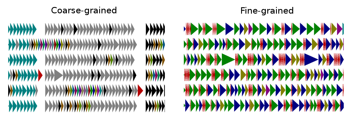
Figure 3.1: Scheduling trace of the task-based approach; Tasks $\mathcal{T}_{M}$ (red color) are processing aggregated or single $E_{2}$ events while tasks $\mathcal{T}_{S}$ (other colors) compute private work on partitioned sub-domains. As coarse-grained tasks control a higher number of dependencies, blocking may occur. Fine-grained scheduling leads to better interleaving but higher overhead cost.

4 Computational experiments

In the following section we present results of computational experiments of our simulator. The following measurements were obtained on Sandy; a Dell Power Edge R820 computer system equipped with four Intel Xeon E5-4650 processors and 8 cores on each socket. We restricted the execution to available physical cores, as timing results on hyper-threads were strongly fluctuating. We begin with a real-world simulation using animal movement data on national scales, followed by a synthetic benchmark for scalability at varying connectivity load, and we conclude with a compute-intensive parameter estimation example.

4.1 National scale simulation of VTEC bacteria spread

Verotoxigenic Escherichia coli O157:H7 (VTEC O157) is a zoonotic bacterial pathogen with the potential to cause severe disease in humans, notably children [43, 44, 45]. Cattle infected with VTEC O157 are an important reservoir for the bacteria and they shed the bacteria in the feces without any signs of clinical disease [46]. Reducing the prevalence of infected cattle in the population could potentially reduce the number of human cases. However, the epidemiology of VTEC O157 in cattle is complex and targeted interventions to control the bacteria require a thorough understanding of the source and transmission routes [46].

To explore the feasibility of national scale simulations to improve the understanding of the underlying disease spread mechanisms, we have created a model of the VTEC O157 dynamics, using the presented framework. European Union legislation requires member states to keep register of bovine animals including the location and the date of birth, movements between holdings, and date of death or slaughter [47, 48]. These records enable data-driven disease spread simulations that include spatio-temporal dynamics of the cattle population with regard to age structures, births, herd size, slaughter, and trade patterns.

The present computational experiment is based on all cattle reports to the Swedish Board of Agriculture over the period 2005-07-01 to 2013-12-31. From these reports, three types of $E_{1}$ external events (enter, exit, aging), and a single type of $E_{2}$ event (animal movements) were condensed. In total there were $\sim 10^{8}$ external events processed during the total runtime of $T=3106$ days. We let each integer in $0,1,\ldots,T$ represent a synchronization window for external events, where in each window $3707\pm 670$ $E_{1}$ events and $235\pm 104$ $E_{2}$ events were processed. A subset of the spatial network consisting of $N_{n}=37221$ nodes is visualized in Figure 4.1.

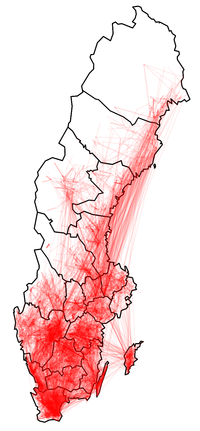
Figure 4.1: Visualization of cattle movements in the VTEC O157 disease spread simulation (§4.1). The arcs shown are a random subset of the complete dataset of $\sim 10^{8}$ recorded events. The source of the data is the national cattle register at the Swedish Board of Agriculture.

Most infected cattle shed the bacteria less than 30 days before returning to the susceptible state, but calves shed for a longer period than adult cattle [49, 50]. To capture this we let the intensity of the transitions between the states depend on the $j$th age category,

$$\begin{array}[]{rl}S_{j}&\xrightarrow{\eta_{j}}I_{j},\\ I_{j}&\xrightarrow{\gamma_{j}}S_{j}.\end{array}$$ (4.3)

The rate for a susceptible individual on the $i$th node to become infected per unit of time is given by

$$\eta_{j}=u\upsilon_{j}\varphi_{i}(t),$$ (4.4)

for $i=1,\ldots,N_{n}$ and $j\in\{\textit{calves},\textit{young stock},\textit{adults}\}$. In turn, the expected time an infected individual is in an infected state before it returns to the susceptible state is

$$\gamma_{j} =\frac{u}{\delta_{j}},$$ (4.5)

where $\delta=[28,25,22]$ and $\upsilon=[8,7,1]\times 10^{-3}$ are age-dependent constants. The factor $u$ can be understood as a time-scale and is difficult to estimate accurately; in our experiments it is in fact varied such that $u=1$ closely resembles the parameterization of the model found in [51].

Finally, the continuous variable $\varphi_{i}$ represents the environmental bacterial concentration that asserts an infectious pressure on each individual at the $i$th node. A suitable model is given by

$$\frac{d\varphi_{i}}{dt}=\frac{\alpha\sum_{j}I_{i,j}(t)}{\sum_{j}S_{i,j}(t)+I_{i,j}(t)}-\beta(t)\varphi_{i}(t).$$ (4.6)

Again, $i=1,\ldots,N_{n}$ are the nodes and $S_{i,j}$ and $I_{i,j}$ refers to the number of susceptible and infected individuals in the $j$th age compartment at the $i$th node, respectively. The constant $\alpha$ is the average shedding rate of bacteria to the environment per infected individual, while $\beta$ captures the decay and removal of bacteria. In our experiments we used the constant value $\alpha=1$ while $\beta(t)$ varied according to the season,

$$\beta(t)=\left\{\begin{array}[]{lr}\log(2)/14:&0\leq(t\bmod{365})\leq 91\\ \log(2)/26:&91<(t\bmod{365})\leq 182\\ \log(2)/20:&182<(t\bmod{365})\leq 273\\ \log(2)/12:&273<(t\bmod{365})\leq 364\end{array}\right.$$ (4.7)

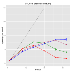
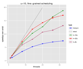
Figure 4.2: Performance measurements of the VTEC O157 model simulation on Sandy at varying scheduling approaches, task sizes, and scale factor $u$. The number of tasks $k$ is chosen to be proportional to the number of threads $c$. In the Open MP parallelization (“forkjoin”), cross-boundary events are processed entirely in serial. Error bars represent the standard error in mean (n=10).

We first parallelized the simulation by spreading tasks $\mathcal{T}_{S}$ over multiple cores using Open MP and serially processing the intermediate $\mathcal{E}^{c}_{2}$ events, hereafter referred to as the fork-join approach. Next, we simulated the model using the task-based approach, scheduling tasks with coarse-grained and fine-grained policies as described in §3.6. We chose the number of sub-domains $k$ to be a multiple of the number of threads $c$. Note that this is also the number of tasks $\mathcal{T}_{S}$ scheduled for each time window $\Delta t$. As a higher factor $u$ creates a higher load for the tasks $\mathcal{T}_{S}$, we vary $u$ to inspect boundary regions of the parallel performance.

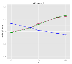
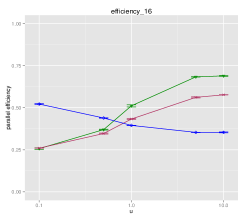
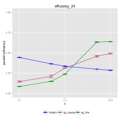
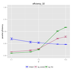
Figure 4.3: Parallel efficiency of the VTEC O157 model simulation on Sandy at varying factor $u$. For all task-based approaches the task size $k=16c$. Error bars represent the standard error in mean (n=10).

The scaling of the different approaches is shown in Figure 4.2. For the case of $u=1$, we find that task sizes are too small to be efficient in both task-based approaches, and thus the fork-join approach reaches a higher efficiency.

At $u=10$, we observe that coarse-grained processing performs better than the fork-join parallelization, optimally at task sizes $k=16c$ and $k=32c$. In the case of fine-grained task processing, we found that the choice of $k$ has a strong impact on the performance scaling. While all task densities scale strongly at a lower thread count, only the $k=16c$ density reaches a high efficiency of $0.58$ at full thread consumption. Thus the efficiency is more than doubled in comparison to the efficiency of the fork-join parallelization, which was found to be 0.23.

The dependency of the parallel efficiency on the factor $u$ is further detailed in Figure 4.3. We observe that scheduling overhead and small task sizes prohibit a high efficiency of both task-based approaches if $u<1$ while the full potential of the approaches is extractable at $u>1$ and a larger thread count. Note that the thread affinity of tasks was varied throughout the performed experiments in order to investigate the impact of data locality.

We further present a set of characteristics of the coarse-grained and fine-grained simulations in Table 4.1 and 4.2. As shown in Table 4.1, the granularity of the fine-grained task $\mathcal{T}_{M}$ is $\sim 1/30$ of the granularity of the coarse-grained task $\mathcal{T}_{M}$, however the task needs to be scheduled about $235$ times more often throughout the simulation run.

On the other hand, the advantage of the fine-grained scheduling is emphasized by the measurements shown in Table 4.2; the average waiting time to fulfill the dependencies for the fine-grained $\mathcal{T}_{M}$ is $44-108\times$ lower than for the coarse-grained $\mathcal{T}_{M}$. This is explained by the larger number of dependencies associated to the coarse-grained $\mathcal{T}_{M}$ which is growing with the partitioning $k$.

The resulting execution trace is also visualized in Figure 3.1, where we show that fine-grained $\mathcal{T}_{M}$ tasks interleave more densely with tasks $\mathcal{T}_{S}$, thus leading to lower idle times and higher parallel efficiency. The percentage of total work spent on the processing of tasks, the synchronization of worker threads, as well as the time spent waiting for fulfilled dependencies are shown in Figure 4.4 for the $u=10$ configuration.

For further details of the scheduling performance of the SuperGlue library in regards to the task sizes and the number of dependencies, we like to refer the reader to the benchmarks available in [28].

	Task granularities ($10^{3}$ cycles)			Number of tasks
$k$	$\mathcal{T}_{S}$	$\mathcal{T}_{M}$ coarse	$\mathcal{T}_{M}$ fine	$\mathcal{T}_{S}$	$\mathcal{T}_{M}$ coarse	$\mathcal{T}_{M}$ fine
256	596 $\pm$ 799	314 $\pm$ 132	11 $\pm$ 5.2	794112	3102	731889
512	301 $\pm$ 461	328 $\pm$ 145	11 $\pm$ 5.2	1588224	3102	731889
1024	152 $\pm$ 294	327 $\pm$ 145	11 $\pm$ 5.2	3176448	3102	731889

Table 4.1: Average task granularity $\pm$ the standard deviation, and the total number of tasks created during the simulation at a given partitioning $k$.

	Waiting for dependencies ($10^{3}$ cycles)				Number of dependencies
$k$	$\mathcal{T}_{S}$ coarse	$\mathcal{T}_{M}$ coarse	$\mathcal{T}_{S}$ fine	$\mathcal{T}_{M}$ fine	$\mathcal{T}_{S}$	$\mathcal{T}_{M}$ coarse	$\mathcal{T}_{M}$ fine
256	15 $\pm$ 10	550 $\pm$ 200	12.5 $\pm$ 5	12.5 $\pm$ 5	1	146 $\pm$ 33	2
512	12.5 $\pm$ 5	850 $\pm$ 200	12.5 $\pm$ 5	12.5 $\pm$ 5	1	202 $\pm$ 58	2
1024	12.5 $\pm$ 5	1350 $\pm$ 500	11 $\pm$ 4	11.5 $\pm$ 4	1	248 $\pm$ 83	2

Table 4.2: Maximum $\pm$ full-width-half-maximum of the (right-skewed) histogram of waiting times for fulfilled task dependencies, and the average amount $\pm$ standard deviation of dependencies assigned to tasks at each discrete time interval $[t_{n},t_{n+1}]$, at a given partitioning $k$ on 32 computing cores.

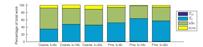
Figure 4.4: Percentage of total work spent on processing of tasks, synchronization (“sync”), and time spent waiting for dependencies (“idle”) for various scheduling policies when measured on 32 cores. Note that the relation of work to overhead agrees well with Figure 4.2.

4.2 Synthetic benchmark

The results in §4.1 indicate a delicate performance dependency on the balance between the local events and the effective connectivity of the network. To further investigate this a synthetic benchmark with a fixed load of local events was created. This model consists of two compartments $S$ and $I$ only, both residing on $N_{n}=1000$ nodes. The transitions are simply

$$\begin{array}[]{rl}S&\xrightarrow{1}I,\\ I&\xrightarrow{1}S,\end{array}$$ (4.10)

where the initial population size of each compartment $I_{i}$ and $S_{i}$ was set to 1000. This model is considered at times $t=[0,\Delta t,2\Delta t,\ldots T]$, with $\Delta t=1$ and $T=1000$, thus generating about 2000 local events per synchronization time window $\Delta t$ and node $i$.

The nodes were arranged into $k$ sub-domains and a total of $\rho k(k-1)/2$ distinct $E_{2}$ events were generated at the end of each time window, each connecting two randomly sampled nodes $\mathbb{X}^{(i)}$ and $\mathbb{X}^{(j)}$ belonging to different sub-domains. Hence $\rho=1$ means that all sub-domains have to communicate with all other sub-domains at each synchronization point. The number of tasks for the coarse-grained and fine-grained approach was set to the number of threads ($k=c$).

The measurements obtained on the Sandy computer system at full thread consumption are presented in Figure 4.5. The parallel efficiency of all methods lies at $\sim 0.7$ for $\rho\leq 0.1$ and remains there even when $\rho\to 0$ and so we deduce that the problem is memory bound. The coarse-grained task-based implementation and the fork-join approach scale very similarly with increasing connectivity $\rho$. The fine-grained task-based approach attains the highest parallel efficiency at $\rho\leq 0.1$, but the performance drops at a higher global connectivity. This phenomenon arises because each $\mathcal{T}_{M}$-task creates dependencies on two subsequent $\mathcal{T}_{S}$-tasks at every synchronization window, thus creating a higher overhead and limiting asynchronous task execution.

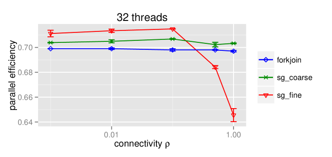
Figure 4.5: Parallel efficiency for the different methods on the synthetic benchmark. Error bars represent the standard error in mean (n=10).

4.3 Feasibility of parameter estimation

A usually very compute intensive load case is the fitting of model parameters, typically using numerical optimization of some kind. The problem can briefly and ideally be described as follows; unknown is the set of parameters $k^{*}$ and an observed time-series of data $\mathbb{X}(t;\;k^{*})$. The parameters $k^{*}$ are estimated by repeatedly simulating a whole family of trajectories with parameters $k$, where $k$ is modified until input data and simulations match up in some suitable sense. The framework’s feasibility of fitting an epidemiological model is of course very important, since the modeling process at some point or the other will involve calibration of parameters with respect to reference data.

To demonstrate the feasibility of parameter estimation in the current context, we use the epidemiological model introduced in §4.1 and first identify the set of parameters $[k_{1},k_{2},k_{3}]$ that have a high degree of observability. A suitable such set is

$$k_{j}=\upsilon_{j}\delta_{j},\leavevmode\nobreak\ j\in\{\textit{calves, young stock, adults}\}.$$ (4.11)

We let a reference solution be given by a single trajectory $\mathbb{X}(t;\;k^{*})$, with $\delta^{*}=[28,25,22]$, $\upsilon=[8.8,3.2,1]\times 10^{-3}$, and with $\alpha$ and $\beta=\beta(t)$ as in §4.1.

To obtain a robust procedure, some kind of smoothing statistics should be considered. We chose to aggregate counts of animals in neighboring nodes into larger regions. To be precise, the overall domain was divided into 21 areas (coinciding with the Swedish county codes), after which the goodness of fit $G(k)$ was defined by

$$G(k)^{2} =\int_{0}^{T}\sum_{j}\left\|\bar{\textbf{x}}_{j}(t;\;k)-\sum_{l\in C(j)}\mathbb{X}^{(l)}(t;\;k^{*})\right\|^{2}\,dt,$$ (4.12)

with

$$\bar{\textbf{x}}_{j}(t;\;k) =\frac{1}{N}\sum^{N}_{i=1}\bar{x}_{j}^{i}(t;\;k),$$ (4.13)

and where the individual sample trajectories are given by

$$\bar{x}_{j}^{i}(t;\;k) =\sum_{l\in C(j)}\mathbb{X}^{(l)}(t;\;k,\;\omega_{i}),$$ (4.14)

where $N$ is the number of trajectories and $C(j),j\in\{1,\ldots,21\}$ is the set of nodes $\mathbb{X}^{(l)}$ that belong to county $j$. To quantify the uncertainty in $G(k)$ we compute the variance as

$$VG(k)^{2} =\int_{0}^{T}\sum_{j}\bar{\sigma}^{2}_{j}(t;\;k)\,dt,$$ (4.15)

where

$$\bar{\sigma}^{2}_{j}(t;\;k) =\frac{1}{N-1}\sum_{i}\|\bar{x}_{j}^{i}(t;\;k)-\bar{\textbf{x}}_{j}(t;\;k)\|^{2},$$ (4.16)

and use $\pm 2VG(k)/\sqrt{N}$ as a measure of the uncertainty.

Next, the parameter estimation problem is approached by solving the minimization problem

$$\hat{k} =\arg\min_{k}G(k)^{2}.$$ (4.17)

In practice we make use of the Pattern Search routine in [52], which conceptually resembles the Golden Section search [53] in its narrowing of the search-space. The numerical optimization routine evaluates (4.12) until the residual error reaches a defined threshold. In our tests we varied the initial guess of the parameters $k_{0}$ but found that the results did not vary substantially. In the results below, we conveniently put $k_{0}=1.6k^{*}$.

Since an increasing number of trajectories yields better estimates of the mean and variance, we simulate using different number of trajectories. We measure the total solver time on 12 and 32 computing cores, respectively, and we let the total number of iterations to be $N=20$ in all cases. The results are presented in Table 4.3 where the relative residual is defined as

$$R(k) =\frac{|G({k})-G(k^{*})|}{|G(k^{*})|}.$$ (4.18)

The optimization landscape of the goal function (4.12), and hence the definiteness of the setup itself, is visualized in Figure 4.6. Due to the simple bisection search behavior of the numerical routine, the obtained parameters $k$ are in fact the same for all displayed cases, although the relative residuals differ considerably.

Trajectories	Rel. residual	Time (c=12)	Time (c=32)
10	0.1738	46.6 min	30.2 min
20	0.0900	94.2 min	61.5 min
40	0.0363	189.3 min	123.7 min

Table 4.3: Solver time of the parameter estimation problem on 12 and 32 cores, respectively, and using a different number of simulated trajectories.

Note that the obvious approach of parallelization by computing the $N$ independent trajectories using separate threads by a sequential algorithm is unfavorable here, for two related reasons. Firstly, each executable needs to store a rather large state space in working memory. Secondly, each simulation must also access the complete database of externally scheduled events.

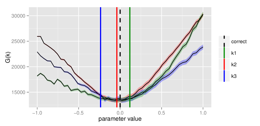
Figure 4.6: Goal function $G(k)$ in the form of confidence intervals $G(k)\pm 2VG(k)$, visualized for each parameter $k_{j}$, $j=\{1,2,3\}$, when the other parameters $k_{i}$, $i\neq j$, are held at the target value $k^{*}_{i}$. Vertical lines indicate the target $k^{*}$ and the obtained estimates $k_{1\ldots 3}$. The parameter ranges have been normalized for ease of comparison.

5 Conclusions

Modeling and simulation are important in designing surveillance and control of livestock diseases and of major economic importance. However, various pathogens require different models to capture the disease dynamics and transmission routes. Moreover, an increasing amount of epidemiologically relevant data is becoming available. We have adressesed these challenges and present a flexible and efficient computational framework for modeling and simulation of disease spread on a national scale. The simulation involves two parts. Firstly, the algorithm evolves stochastic dynamics of the disease process. Secondly, a list processor incorporates database events such as entering, exit, or movement of individuals into the model state. The framework is highly flexible in that most conceivable epidemiological models are either directly expressible, or the framework may be straightforwardly extended to encompass also non-standard models. As a concrete example it would be relatively easy to include intervention strategies such as vaccination programs in order to simulate the impact on the global dynamics.

We have explored different strategies to parallelize the simulator on multi-socket architectures. Firstly, we decomposed the spatial information and the list of deterministic events. We then observed that the decomposed problem can be simulated at a high parallel efficiency, which is limited only by the processing of cross-boundary events. We then created three parallel implementations of the simulator core; we used Open MP to only parallelize private computations in a fork-join fashion, while cross-boundary events were processed in serial. Two further implementations use a dependency-aware task scheduler to create execution traces that interleave cross-boundary events and private computations with respect to their dependencies. We find that this strategy allows us to exploit shared-memory parallelism at a higher degree than the fork-join approach if task sizes are sufficiently large. We benchmark this approach using the SuperGlue task library, but present a set of scheduling rules defining the parallel simulator on general terms, thus allowing it to be implemented also with other dependency-aware task libraries.

We benchmarked our simulator using a model of the spatio-temporal spread of VTEC O157 bacteria in the Swedish cattle population. The model contains 37221 nodes and evolves $\sim 10^{8}$ external events from register data. We found that at a low private work load, the fork-join approach performs best, mainly due to the scheduling overhead of the task-based approaches. For higher private work loads, the simulation benefits from task-based computing, doubling the parallel efficiency on 32 cores in comparison to the fork-join approach.

To further inspect the performance dependency on network properties, we constructed a synthetic benchmark where cross-boundary events were generated randomly. Here we found that the performance of the fork-join approach and the coarse-grained task approach scales well with a growing amount of cross-boundary events. Notably, the performance of the fine-grained task processing depends more strongly on the connectivity of boundary crossing events, thus favoring a more fragmented network.

In a final example we used the simulator to carry out an experimental parameter fitting within the VTEC O157 bacteria spread model. We emphasize the high computational complexity of this task with multiple unknown parameters to fit and the need to use several full simulation runs to evaluate each parameter candidate. A similar load case results when different intervention strategies are to be evaluated. For example, even when several interventions reduce the infectious spread globally, a policy maker could be interested in finding the most cost-efficient strategy. With this work, we provide a powerful, highly general and freely available software, that can contribute to a rapid and more efficient development of realistic large-scale epidemiological models.

Future research will encompass studies of larger inverse problems, including more realistic data input, and more complex dynamics. Yet another point for future study is the scalability of the task-based approach in a distributed environment.

Appendix A Algorithms

Algorithm 1 Sequential simulation loop

1:  Initialize: Compute all stochastic rates $\omega_{i}$ in all nodes $\mathbb{X}^{(i)},i=1,\ldots,N_{n}$.

2:  while $t<T_{End}$ do

3:     for all nodes i=1 to $N_{n}$ do

4:        while $t<(t_{n}+\Delta t)$ do

5:           Compute the sum $\lambda$ of all transition intensity functions.

6:           Sample the next stochastic event time by $\tau=-log(rand)/\lambda$ using a uniformly distributed random variable $rand$.

7:           Determine which event happened. Sample the next event (by inversion); find $n$ such that $\sum_{j=1}^{n-1}\omega_{j}(\mathbb{X}^{(i)})<\lambda\,\mbox{rand}\leq\sum_{j=1}^{n}\omega_{j}(\mathbb{X}^{(i)})$

8:           Update the state $\mathbb{X}^{(i)}$ using the stoichiometric matrix $\mathbb{S}$.

9:           Update $\omega_{n}$ using the dependency graph $G$ to recalculate only affected stochastic rates.

10:        end while

11:     end for

12:     $t_{n+1}=t_{n}+\Delta t_{n}$

13:     Incorporate externally defined events in lists $\mathcal{E}_{1,2}$.

14:     Loop over all nodes $\mathbb{X}^{(i)}$ and update the continuous state variable $Y^{(i)}$.

15:  end while

Algorithm 2 Parallel simulation loop

1:  Initialize: Decompose the nodes $V$ into $k$ sub-domains $V_{k}$. Re-arrange the external events of type $E_{1}$ into private lists $\mathcal{E}^{k}_{1}$ of each sub-domain $k$, where all $n$ affected nodes $\mathbb{X}_{n}\in V_{k}$. Further divide all $E_{2}$ events into the private list $\mathcal{E}^{k}_{2}$ or the list of domain-crossing events $\mathcal{E}^{c}_{2}$.

2:  while $t<T_{End}$ do

3:     for all i=1 to $k$ do

4:        % Parallel task $\mathcal{T}_{S}$;

5:        Execute line 14 of Algorithm 1 for all nodes in sub-domain $V_{k}$ if $n>1$.

6:        Execute lines 3-10 of Algorithm 1 for all nodes in sub-domain $V_{k}$ evolving time $t\in[t_{n},t_{n}+\Delta t]$.

7:        Execute line 13 of Algorithm 1 for all events in lists $\mathcal{E}^{k}_{1}$ and $\mathcal{E}^{k}_{2}$ at time $t\in[t_{n},t_{n}+\Delta t]$.

8:        % End of parallel task $\mathcal{T}_{S}$

9:     end for

10:     % Parallel task $\mathcal{T}_{M}$;

11:     Execute line 13 of Algorithm 1 for all events in the list $\mathcal{E}^{c}_{2}$ at time $t\in[t_{n}\leavevmode\nobreak\ (t_{n}+\Delta t)]$.

12:     % End of parallel task $\mathcal{T}_{M}$;

13:     $t_{n+1}=t_{n}+\Delta t_{n}$

14:  end while

References

- [1] L Hasonova and I Pavlik. Economic impact of paratuberculosis in dairy cattle herds: a review. Vet Med-Czech, 51(5):193–211, 2006.
- [2] T J D. Knight-Jones and J. Rushton. The economic impacts of foot and mouth disease - what are they, how big are they and where do they occur? Prev Vet Med, 112(3-4):161–173, 2013.
- [3] P Willeberg, T Grubbe, S Weber, K Forde-Folle, and C Dubé. The world organisation for animal health and epidemiological modelling: background and objectives. Rev Sci Tech, 30(2):391–405, 2011.
- [4] E. Brooks-Pollock, M.C.M. de Jong, M.J. Keeling, D. Klinkenberg, and J.L.N. Wood. Eight challenges in modelling infectious livestock diseases. Epidemics, 10:1–5, 2015.
- [5] Lorenzo Pellis, Frank Ball, Shweta Bansal, Ken Eames, Thomas House, Valerie Isham, and Pieter Trapman. Eight challenges for network epidemic models. Epidemics, 10:58–62, 2015.
- [6] Priscilla E. Greenwood and Luis F. Gordillo. Stochastic epidemic modeling. In Mathematical and Statistical Estimation Approaches in Epidemiology, pages 31–52. Springer Netherlands, 2009.
- [7] Matt J Keeling. Models of foot-and-mouth disease. Proc R Soc B, 272(1569):1195–1202, 2005.
- [8] M. A. Stevenson, R. L. Sanson, M. W. Stern, B. D. O’Leary, M. Sujau, N. Moles-Benfell, and R. S. Morris. InterSpread plus: a spatial and stochastic simulation model of disease in animal populations. Prev Vet Med, 109(1–2):10–24, 2013.
- [9] Neil Harvey, Aaron Reeves, Mark A. Schoenbaum, Francisco J. Zagmutt-Vergara, Caroline Dubé, Ashley E. Hill, Barbara A. Corso, W. Bruce McNab, Claudia I. Cartwright, and Mo D. Salman. The north american animal disease spread model: A simulation model to assist decision making in evaluating animal disease incursions. Prev Vet Med, 82(3–4):176–197, 2007.
- [10] Naoki Masuda and Petter Holme. Predicting and controlling infectious disease epidemics using temporal networks. F1000prime Rep, 5, 2013.
- [11] Mark DF Shirley and Steve P Rushton. The impacts of network topology on disease spread. Ecol Complex, 2(3):287–299, 2005.
- [12] K. Büttner, J. Krieter, A. Traulsen, and I. Traulsen. Epidemic spreading in an animal trade network - comparison of distance-based and network-based control measures. Transbound Emerg Dis, 2014.
- [13] Christos G. Cassandras and Stéphane Lafortune. Systems and models. In Introduction to Discrete Event Systems, pages 1–51. Springer US, 2008.
- [14] Richard M. Fujimoto. Parallel discrete event simulation. Commun ACM, 33(10):30–53, 1990.
- [15] Richard M. Fujimoto. Parallel and Distribution Simulation Systems. John Wiley & Sons, Inc., New York, NY, USA, 1st edition, 1999.
- [16] David R. Jefferson. Virtual time. ACM T Progr Lang Sys, 7(3):404–425, 1985.
- [17] Christopher D. Carothers, Kalyan S. Perumalla, and Richard M. Fujimoto. Efficient optimistic parallel simulations using reverse computation. ACM T Model Comput S, 9(3):224–253, 1999.
- [18] P. Heidelberger and D.M. Nicol. Conservative parallel simulation of continuous time Markov chains using uniformization. IEEE Trans Parallel Distrib Syst, 4(8):906–921, August 1993.
- [19] Maciej Drozdowski. Parallel tasks. In Scheduling for Parallel Processing, Computer Communications and Networks, pages 87–208. Springer London, 2009.
- [20] Z. Xiao, B. Unger, R. Simmonds, and J. Cleary. Scheduling critical channels in conservative parallel discrete event simulation. In Proc 13th PADS, pages 20–28, 1999.
- [21] D.M. Nicol and J. Liu. Composite synchronization in parallel discrete-event simulation. IEEE Trans Parallel Distrib Syst, 13(5):433–446, 2002.
- [22] C.L. Barrett, K.R. Bisset, S.G. Eubank, Xizhou Feng, and M.V. Marathe. EpiSimdemics: An efficient algorithm for simulating the spread of infectious disease over large realistic social networks. In Prof of SC 2008, pages 1–12, November 2008.
- [23] Jae-Seung Yeom, A. Bhatele, K. Bisset, E. Bohm, A. Gupta, L.V. Kale, M. Marathe, D.S. Nikolopoulos, M. Schulz, and L. Wesolowski. Overcoming the scalability challenges of epidemic simulations on Blue Waters. In Proc 28th IEEE Int Par Dist Symp, pages 755–764, May 2014.
- [24] Jaspal Subhlok, James M. Stichnoth, David R. O’Hallaron, and Thomas Gross. Exploiting task and data parallelism on a multicomputer. In Proc 4th PPOPP, pages 13–22, New York, NY, USA, 1993. ACM.
- [25] Daan Leijen, Wolfram Schulte, and Sebastian Burckhardt. The design of a task parallel library. In Proc 24th ACM SIGPLAN OOPSLA, pages 227–242, New York, NY, USA, 2009. ACM.
- [26] Alejandro Duran, Eduard Ayguadé, Rosa M. Badia, Jesús Labarta, Luis Martinell, Xavier Martorell, and Judit Planas. OmpSs: A proposal for programming heterogeneous multi-core architectures. Parallel Process Lett, 21(02):173–193, 2011.
- [27] Cédric Augonnet, Samuel Thibault, Raymond Namyst, and Pierre-André; Wacrenier. StarPU: A unified platform for task scheduling on heterogeneous multicore architectures. Concurr Comp-Pract E, 23(2):187–198, 2011.
- [28] M. Tillenius. SuperGlue: A shared memory framework using data versioning for dependency-aware task-based parallelization. SIAM J Sci Comput, 37(6):C617–C642, January 2015.
- [29] W. O. Kermack and A. G. McKendrick. A contribution to the mathematical theory of epidemics. Proc Roy Soc A, 115:700–721, 1927.
- [30] S. Engblom. Strong convergence for split-step methods in stochastic jump kinetics. SIAM J Numer Anal, 53(6):2655–2676, 2015.
- [31] Daniel T. Gillespie. Exact stochastic simulation of coupled chemical reactions. J Phys Chem, 81(25):2340–2361, 1977.
- [32] Michael A. Gibson and Jehoshua Bruck. Efficient exact stochastic simulation of chemical systems with many species and many channels. J Phys Chem A, 104(9):1876–1889, 2000.
- [33] Stefan Engblom, Lars Ferm, Andreas Hellander, and Per Lötstedt. Simulation of stochastic reaction-diffusion processes on unstructured meshes. SIAM J Sci Comput, 31(3):1774–1797, 2009.
- [34] Brian Drawert, Stefan Engblom, and Andreas Hellander. URDME: a modular framework for stochastic simulation of reaction-transport processes in complex geometries. BMC Sys Biol, 6(1):76, 2012.
- [35] Konstantin Andreev and Harald Räcke. Balanced graph partitioning. In Proc 16th ACM SPAA, SPAA ’04, page 120–124, New York, NY, USA, 2004. ACM.
- [36] Azzam Haidar, Stanimire Tomov, Jack Dongarra, Raffaele Solcà, and Thomas Schulthess. A novel hybrid CPU–GPU generalized eigensolver for electronic structure calculations based on fine-grained memory aware tasks. Int J High Perform C, 28(2):196–209, 2014.
- [37] Qingyu Meng and Martin Berzins. Scalable large-scale fluid–structure interaction solvers in the uintah framework via hybrid task-based parallelism algorithms. Concurr Comp-Pract E, 26(7):1388–1407, 2014.
- [38] L. A. Berry, W. Elwasif, J. M. Reynolds-Barredo, D. Samaddar, R. Sanchez, and D. E. Newman. Event-based parareal: A data-flow based implementation of parareal. J Comp Phys, 231(17):5945–5954, 2012.
- [39] Apostolos Gerasoulis and Tao Yang. On the granularity and clustering of directed acyclic task graphs. IEEE Trans Parallel Distrib Syst, 4(6):686–701, June 1993.
- [40] J.M. Perez, R.M. Badia, and J. Labarta. A dependency-aware task-based programming environment for multi-core architectures. In 2008 IEEE Conf Clust Comput, pages 142–151, 2008.
- [41] OpenMP Architecture Review Board. OpenMP 4.0 Application Program Interface, 7 2013. Page 117, Lines 14–15.
- [42] Afshin Zafari, Martin Tillenius, and Elisabeth Larsson. Programming models based on data versioning for dependency-aware task-based parallelisation. In Proc 15th Comput Sci Eng, pages 275–280, Washington, DC, USA, 2012. IEEE Computer Society.
- [43] M. A. Karmali, M. Petric, C. Lim, P. C. Fleming, and B. T. Steele. Escherichia coli cytotoxin, haemolytic-uraemic syndrome, and haemorrhagic colitis. Lancet, 2(8362):1299–1300, 1983.
- [44] M. A. Karmali, B. T. Steele, M. Petric, and C. Lim. Sporadic cases of haemolytic-uraemic syndrome associated with faecal cytotoxin and cytotoxin-producing escherichia coli in stools. Lancet, 1(8325):619–620, 1983.
- [45] L. W. Riley, R. S. Remis, S. D. Helgerson, H. B. McGee, J. G. Wells, B. R. Davis, R. J. Hebert, E. S. Olcott, L. M. Johnson, N. T. Hargrett, P. A. Blake, and M. L. Cohen. Hemorrhagic colitis associated with a rare escherichia coli serotype. New Eng Jo Med, 308(12):681–685, 1983.
- [46] Dale Hancock, Tom Besser, Jeff Lejeune, Margaret Davis, and Dan Rice. The control of VTEC in the animal reservoir. Int J Food Microbiol, 66(1-2):71 – 78, 2001.
- [47] Anonymous. Regulation (EC) No 1760/2000 of the European Parliament and of the Council of 17 July 2000 establishing a system for the identification and registration of bovine animals and regarding the labelling of beef and beef products. OJEU, L 204:1–10, 2000.
- [48] Anonymous. Commission Regulation (EC) No 911/2004 of 29 April 2004 implementing Regulation (EC) No 1760/2000 of the European Parliament and of the Council as regards eartags, passports and holding registers. OJEU, L 163:65–70, 2004.
- [49] W. C. Cray and H. W. Moon. Experimental infection of calves and adult cattle with Escherichia coli O157:H7. Appl Environ Microbiol, 61(4):1586–1590, 1995.
- [50] Margaret A. Davis, Daniel H. Rice, Haiqing Sheng, Dale D. Hancock, Thomas E. Besser, Rowland Cobbold, and Carolyn J. Hovde. Comparison of cultures from rectoanal-junction mucosal swabs and feces for detection of Escherichia coli O157 in dairy heifers. Appl Environ Microbiol, 72(5):3766–3770, 2006.
- [51] Stefan Widgren, Stefan Engblom, Pavol Bauer, Jenny Frössling, Ulf Emanuelson, and Anne Lindberg. Data-driven network modeling of VTEC O157 transmission in Swedish cattle using complete population movement data, 2016. Submitted.
- [52] Robert Hooke and T. A. Jeeves. Direct search: Solution of numerical and statistical problems. J ACM, 8(2):212–229, 1961.
- [53] J. Kiefer. Sequential minimax search for a maximum. Proc Amer Math Soc, 4(3):502–506, 1953.