Flux Phase in Bilayer $t-J$ Model: Time-Reversal Symmetry Breaking Surface State without Spontaneous Magnetic Field

Abstract

We study surface states of high-$T_{C}$ cuprate superconductor YBCO using the bilayer $t-J$ model. Calculations based on the Bogoliubov de Gennes method show that a flux phase that breaks time-reversal symmetry (${\cal T}$) may arise near a (110) surface where the $d_{x^{2}-y^{2}}$-wave superconductivity is strongly suppressed. It is found that the flux phase in which spontaneous magnetic fields in two layers have opposite directions may be stabilized in a wide region of doping rate, and split peaks in the local density of states appear. Near the surface, spontaneous magnetic field may not be observed experimentally, because the contributions from two layers essentially cancel out. This may explain the absence of local magnetic field near the (110) surface of YBCO, for which the sign of ${\cal T}$ violation has been detected.

1 Introduction

In high-$T_{C}$ cuprate superconductors, spontaneous violation of time-reversal symmetry (${\cal T}$) has been observed in various kinds of experiment.[1, 2, 3, 4] One of the famous example is the peak splitting of zero bias conductance in ab-oriented YBCO/insulator/Cu junction.[1] This has been interpreted as a consequence of the occurrence of second superconducting (SC) order parameter (OP) near the surface, which has symmetry different from that in the bulk.[5, 6, 7] For this type of surface state, spontaneous current would flow along the surface, and a magnetic field should be generated locally. However, experimental evidence for such magnetic fields is still controversial.[8, 9]

The present author has studied the (110) surface state of high-$T_{C}$ cuprates based on the Bogoliubov-de Gennes (BdG) method applied to a single-layer $t-J$ model, and found that a different kind of ${\cal T}$-breaking surface state, flux phase, can occur.[10, 11] The flux phase is a mean-field solution to the $t-J$ model in which staggered currents flow and the flux penetrates a plaquette in a square lattice.[12] This state has free energy higher than that of the $d_{x^{2}-y^{2}}$-wave SC state except very near half filling, so that it is only a metastable state in uniform systems.[13, 14, 15, 16] Near (110) surfaces $d_{x^{2}-y^{2}}$-wave SC state is strongly suppressed, and then the flux phase may arise locally leading to a ${\cal T}$-breaking surface state. However, the doping region in which ${\cal T}$ violation occurs was much narrower than that observed experimentally in YBCO, if we use an effective single-layer model.[10, 11]

Later reexamination using a bilayer $t-J$ model that describes the electronic states of YBCO more accurately have shown that the flux phase may occur as a metastable state in a doping region much wider than that for the effective single-layer model.[17] For the bilayer $t-J$ model, there may be two types of flux phase in which the directions of the flux in two layers are the same or opposite, and a phase transition occurs from the latter to former as the doping rate increases.[17] We call the former (latter) one as a type A (B) flux phase. If the type B flux phase occurs near the (110) surface, the spontaneous magnetic field should be very small, since the contributions from two layers essentially cancel out. This may explain why no magnetic field is observed in some experiments for the (110) surface state of YBCO.

In this paper, we study the (110) surface states of YBCO system that are described by the bilayer $t-J$ model. Spatial variations of the OPs are treated using the BdG method[18], and we will show that the flux phase can occur in a wide region of the doping rate when the SC order is suppressed. The local density of states (LDOS) is also examined to see whether the splitting of the zero-energy peak occurs in agreement with experimental results.

This paper is organized as follows. In Sect. 2 the model is presented and the BdG equations are derived. Results of numerical calculations are described in Sect. 3, and Sect. 4 is devoted to summary.

2 Bogoliubov de Gennes Equations

We consider the bilayer $t-J$ model on a square lattice whose Hamiltonian is given by $H=H_{1}+H_{2}+H_{\perp}$ with

$$\displaystyle H_{i}= \displaystyle-\sum_{j,\ell,\sigma}t_{j\ell}{\tilde{c}}^{(i)\dagger}_{j\sigma}{\tilde{c}}^{(i)}_{\ell\sigma}+J\sum_{\langle j,\ell\rangle}{\bf S}^{(i)}_{j}\cdot{\bf S}^{(i)}_{\ell},\ \ \ (i=1,2)$$ (1)

$$H_{\perp}= \displaystyle-\sum_{j,\ell,\sigma}t_{j\ell}^{\perp}\Big{(}{\tilde{c}}^{(1)\dagger}_{j\sigma}{\tilde{c}}^{(2)}_{l\sigma}+h.c.\Big{)}+J_{\perp}\sum_{j}{\bf S}^{(i1}_{j}\cdot{\bf S}^{(2)}_{j},$$ (2)

where the transfer integrals (in plane) $t_{j\ell}$ are finite for the first- ($t$), second- ($t^{\prime}$), and third-nearest-neighbor bonds ($t^{\prime\prime}$), or zero otherwise. $J$ $(J_{\perp})$ is the inplane (interplane) antiferromagnetic superexchange interaction, and $\langle j,\ell\rangle$ denotes nearest-neighbor bonds.[19] The interplane transfer integrals $t^{\perp}_{j\ell}$ are chosen to reproduce the dispersion in $k$ space,[20] $t^{\perp}_{k}=-t^{\perp}_{0}(\cos k_{x}-\cos k_{y})^{2}$, namely, ”on-site” ($t^{\perp}_{0}$), second- ($t^{\perp}_{2}=-t^{\perp}_{0}/2$) , and third-nearest-nearest-neighbor bonds ($t^{\perp}_{3}=t^{\perp}_{0}/4$) are taken into account.

${\tilde{c}}_{j\sigma}^{(i)}$ is the electron operator for the $i$-th plane in Fock space without double occupancy, and we treat this condition using the slave-boson method[19, 21, 22] by writing ${\tilde{c}}_{j\sigma}^{(i)}=b_{j}^{(i)\dagger}f_{j\sigma}^{(i)}$ under the local constraint $\sum_{\sigma}f_{j\,\sigma}^{(i)\dagger}f_{j\,\sigma}^{(i)}+b_{j}^{(i)\dagger}b_{j}^{(i)}=1$ at every $j$ site. Here $f_{j\sigma}^{(i)}$ ($b_{j}^{(i)}$) is a fermion (boson) operator that carries spin $\sigma$ (charge $e$); the fermions (bosons) are frequently referred to as spinons (holons). The spin operator is expressed as ${\bf S}_{j}^{(i)}=\frac{1}{2}\sum_{\alpha,\beta}f^{(i)\dagger}_{j\alpha}{\bf\sigma}_{\alpha\beta}f_{j\beta}^{(i)}$.

We decouple the Hamiltonian in the following manner.[23, 24] The bond OPs in plane $\sum_{\sigma}\langle f^{(i)\dagger}_{j\sigma}f_{l\sigma}^{(i)}\rangle$ and $\langle b^{(i)\dagger}_{j}b_{l}^{(i)}\rangle$ are introduced, and we denote $\chi_{jl}^{(i)}\equiv\sum_{\sigma}\langle f^{(i)\dagger}_{j\sigma}f_{l\sigma}^{(i)}\rangle$ for nearest-neighbor bonds. The interlayer bond OP is defined as $\chi^{\perp}_{j}\equiv\sum_{\sigma}\langle f^{(1)\dagger}_{j\sigma}f^{(2)}_{j\sigma}\rangle$. Although the bosons are not condensed in purely two-dimensional systems at finite temperature ($T$), they are almost condensed at a low $T$ and for finite carrier doping ($\delta\gtrsim 0.05$). Since we are interested in the low temperature region ($T\leq 10^{-2}J\sim 10$K), we treat holons as Bose condensed. Hence, we approximate $\langle b_{j}^{(i)}\rangle\sim\sqrt{\delta}$ and $\langle b^{(i)\dagger}_{j}b_{l}^{(i)}\rangle\sim\delta$ ($\delta$ being the doping rate), and replace the local constraint with a global one, $\frac{1}{N}\sum_{j,\sigma}\langle f^{(i)\dagger}_{j\sigma}f_{j\sigma}^{(i)}\rangle=1-\delta$, where $N$ is the total number of lattice sites within a plane. This procedure amounts to renormalizing the transfer integrals by multiplying $\delta$, e.g., $t\to t\delta$, etc., and rewriting ${\tilde{c}}_{j\sigma}^{(i)}$ as $f_{j\sigma}^{(i)}$. In a qualitative sense, this approach is equivalent to the renormalized mean-field (MF) theory of Zhang et al.[25] (Gutzwiller approximation). The spin-singlet resonating-valence-bond (RVB) OP on the bond $\langle j,l\rangle$ is given as $\Delta_{j,l}^{(i)}=\langle f_{j\uparrow}^{(i)}f_{l\downarrow}^{(i)}-f_{j\downarrow}^{(i)}f_{l\uparrow}^{(i)}\rangle/2$. The interlayer RVB OP is defined as $\Delta^{\perp}_{j}\equiv\langle f^{(1)}_{j\uparrow}f^{(2)}_{j\downarrow}-f^{(1)}_{j\downarrow}f^{(2)}_{j\uparrow}\rangle/2$. Under the assumption of the Bose condensation of holons, $\Delta_{j,l}$ is equivalent to the SCOP.

We treat a system with a (110) surface, and denote the direction perpendicular (parallel) to the (110) surface as $x$ ($y$). The $x$ coordinate is given as $x_{j}=j_{x}a$ where $a=a^{\prime}/\sqrt{2}$ with $a^{\prime}$ being the lattice constant of the square lattice. In order to describe the Flux phase and the SC state, $\chi^{(i\pm)}_{j}\equiv\chi^{(i)}_{j,j+x\pm y}$ and $\Delta^{(i\pm)}_{j}\equiv\Delta^{(i)}_{j.j+x\pm y}$ are defined for the $i$-th plane. We assume that the system is uniform along the $y$ direction, and consider the spatial variations of OPs only in the $x$ direction. By imposing the periodic boundary condition for the $y$ direction, the Fourier transformation for the $y$ coordinate is performed.[26, 27, 28, 29] (Hereafter we write $j_{x}$ simply as $j$, and take $a=1$.) Then the MF Hamiltonian is written as follows

$${\cal H}_{MF}=\sum_{k}\sum_{j,l}\Psi_{j}^{\dagger}(k){\hat{h}}_{jl}(k)\Psi_{l}(k),$$ (3)

with $\displaystyle\Psi_{j}^{\dagger}(k)=\big{(}f_{j\uparrow}^{(1)\dagger}(k),f_{j\downarrow}^{(1)}(-k),f_{j\uparrow}^{(2)\dagger}(k),f_{j\downarrow}^{(2)}(-k)\big{)}$, and $k$ is the wave number along the $y$ direction. The matrix ${\hat{h}}_{ij}(k)$ is given as

$${\hat{h}}_{jl}(k)=\left(\begin{array}[]{cccc}\xi^{(1)}_{jl}(k)&F^{(1)}_{jl}(k)&\epsilon_{jl}(k)&f_{jl}\\ F_{lj}^{{(1)}*}(k)&-\xi^{(1)}_{lj}(-k)&f^{*}_{jl}&-\epsilon_{lj}^{*}(k)\\ \epsilon_{lj}^{*}(k)&f_{jl}&\xi^{(2)}_{jl}(k)&F^{(2)}_{jl}(k)\\ f_{jl}^{*}&-\epsilon_{jl}(k)&F_{lj}^{{(2)}*}(k)&-\xi^{(2)}_{lj}(-k)\end{array}\right),$$ (4)

where

$$\begin{array}[]{rl}\xi^{(i)}_{jl}(k)=&\displaystyle-\delta_{j,l}(\mu+2t^{\prime}\delta\cos 2k)\\ &\displaystyle-\delta_{j,l-1}\big{[}2t\delta\cos k+\frac{3J}{8}(\chi^{(i+)}_{j}e^{ik}+\chi^{(i-)}_{j}e^{-ik})\big{]}\\ &\displaystyle-\delta_{j,l+1}\big{[}2t\delta\cos k+\frac{3J}{8}((\chi^{(i+)}_{l})^{*}e^{-ik}+(\chi^{(i-)}_{l})^{*}e^{ik})\big{]}\\ &\displaystyle-(\delta_{j,l-2}+\delta_{j,l+2})(t^{\prime}+2t^{\prime\prime}\cos 2k)\delta,\\ &\\ \epsilon_{jl}(k)=&\displaystyle-\delta_{jl}\big{[}(t^{\perp}_{0}+2t^{\perp}_{2}\cos 2k)\delta+\frac{3J_{\perp}}{8}(\chi^{\perp}_{j})^{*}\big{]}\\ &\displaystyle-(\delta_{j,l-2}+\delta_{j,l+2})(t^{\perp}_{2}+2t^{\perp}_{3}\cos 2k)\delta,\\ &\\ F^{(i)}_{jl}(k)=&\displaystyle\frac{3J}{4}\big{[}\delta_{j,l-1}(\Delta^{(i+)}_{j}e^{ik}+\Delta^{(i-)}_{j}e^{-ik})\\ &\displaystyle+\delta_{j,l+1}(\Delta^{(i+)}_{l}e^{-ik}+\Delta^{(i-)}_{l}e^{ik})\big{]},\\ &\\ f_{jl}=&\displaystyle\delta_{jl}\frac{3J_{\perp}}{4}\Delta^{\perp}_{j},\end{array}$$ (5)

with $\mu$ being the chemical potential,

We diagonalize the MF Hamiltonian by solving the following BdG equation for each $k$,

$$\sum_{l}{\hat{h}}_{jl}(k)u_{ln}(k)=E_{n}(k)u_{jn}(k),$$ (6)

where $E_{n}(k)$ and $u_{jn}(k)$ are the energy eigenvalue and the corresponding eigenfunction, respectively, for each $k$. The unitary transformation using $u_{jn}(k)$ diagonalizes the Hamiltonian ${\cal H}_{MF}$, and the OPs and the spinon number at the $j$ site for the layer 1 can be obtained as,

$$\begin{array}[]{rl}\langle n^{(1)}_{j}\rangle=&\displaystyle\frac{1}{N_{y}}\sum_{k,n}\Big{[}\big{|}u_{4j-3,n}(k)\big{|}^{2}f(E_{n}(k))\\ &\displaystyle+\big{|}u_{4j-2,n}(k)\big{|}^{2}\big{[}1-f(E_{n}(k))\Big{]},\\ \chi^{(1\pm)}_{j}=&\displaystyle\frac{1}{N_{y}}\sum_{k,n}\Big{[}u_{4j+1,n}^{*}(k)u_{4j-3,n}(k)e^{\mp ik}f(E_{n}(k))\\ &\displaystyle+u_{4j+2,n}(k)u_{4j-2,n}^{*}(k)e^{\pm ik}(1-f(E_{n}(k)))\Big{]},\\ \Delta^{(1\pm)}_{j}=&\displaystyle\frac{1}{4N_{y}}\sum_{k,n}\Big{[}u_{4j-3,n}(k)u_{4j+2,n}^{*}(k)e^{\mp ik}\\ &\displaystyle+u_{4j-2,n}^{*}(k)u_{4j+1,n}(k)e^{\pm ik}\big{]}\tanh\Big{(}\frac{E_{n}(k)}{2T}\Big{)}\Big{]},\end{array}$$ (7)

where $N_{x}$ ($N_{y}$) and $f$ are the number of lattice sites along the $x$ ($y$) direction within a plane, and the Fermi distribution function, respectively. The OPs and the spinon number for the layer 2 are obtained by replacing the subscripts, $(4j-3)\to(4j-1)$, $(4j-2)\to(4j)$, etc., in Eq. (7). The interlayer OPs are given as,

$$\begin{array}[]{rl}\chi^{\perp}_{j}=&\displaystyle\frac{1}{N_{y}}\sum_{k,n}\Big{[}u_{4j-3,n}^{*}(k)u_{4j-1,n}(k)f(E_{n}(k))\\ &\displaystyle+u_{4j-2,n}(k)u_{4j.n}^{*}(k)(1-f(E_{n}(k)))\Big{]},\\ \Delta^{\perp}_{j}=&\displaystyle\frac{1}{4N_{y}}\sum_{k,n}\Big{[}u_{4j-3,n}(k)u_{4j,n}^{*}(k)+u_{4j-2,n}^{*}(k)u_{4j-1.n}(k)\Big{]}\\ &\displaystyle\times\tanh\Big{(}\frac{E_{n}(k)}{2T}\Big{)}.\end{array}$$ (8)

The $d$- and $s$-wave SCOPs are obtained by combining $\Delta^{(i\pm)}$s: $\Delta^{(i)}_{d}(j)=(\Delta^{(i+)}_{j}-\Delta^{(i-)}_{j}+\Delta^{(i+)}_{j-1}-\Delta^{(i-)}_{j-1})/4$ and $\Delta^{(i)}_{s}(j)=(\Delta^{(i+)}_{j}+\Delta^{(i-)}_{j}+\Delta^{(i+)}_{j-1}+\Delta^{(i-)}_{j-1})/4$.

3 Surface States and Local Density of States

In this section we present the results of numerical calculations for surface states. The procedure of numerical calculations is the following. We diagonalize the Hamitotonian ${\cal H}_{MF}$ with the OPs substituted in matrix elements, and the resulting eigenvalues and eigenfunctions are used to recalculate the OPs. This procedure is iterated until the convergence is reached. For the system size, $N_{x}=200$ and $N_{y}=100$ are used throughout. The band parameters are chosen after Ref. 30; $t/J=2.5$, $t^{\prime}/t=-0.3$, $t^{\prime\prime}/t=0.15$, $t^{\perp}_{0}/t=0.15$, and $J_{\perp}/J=0.1$. These parameters were chosen to reproduce experimental results for YBCO.[30] We restrict ourselves to the case of low temperature, $T=10^{-3}J$ ($\sim 1$K).

The spatial variations of the OPs for $\delta=0.15$ are shown in Figs. 1 and 2. It is seen that the $d$-wave SCOP is suppressed near a (110) surface. The imaginary parts of the bond OPs (Im $\chi$) are finite there, and Im $\chi$ for different layers have opposite signs. This means that the flux phase arises leading to a ${\cal T}$-breaking surface state. Spontaneous current flowing along the surface is given as,

$$J_{y}^{(i)}(j)=\frac{\sqrt{2}\pi t\delta}{\phi_{0}}{\rm Im}\ \chi^{(i+)}_{j},$$ (9)

with $\phi_{0}=h/2e$ being the flux quantum. (In principle, there is a term proportional to the vector potential in $J_{y}$, but we neglect it for simplicity.) From this equation, we see that the directions of the currents and those of the flux in two layers are opposite (type B flux phase). In this case, the spontaneous magnetic field near the surface will be very small, since the contributions from two layers essentially cancel out. Then it will be hard to observe it experimentally. Small imaginary parts of the $s$-wave SCOP (Im $\Delta_{s}$) also appear near the surface, and their signs in two layers are also opposite.

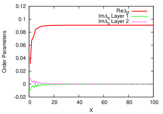
Figure 1: (Color online) Spatial variations of the SCOPs for $\delta=0.15$. Here $x$ is measured in units of lattice spacing $a$. Note that all OPs are nondimensional.

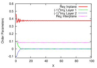
Figure 2: (Color online) Spatial variations of the bond OPs for $\delta=0.15$.

The results for other values of $\delta$ show qualitatively the same behavior; the absolute values of Im $\chi$ are larger (smaller) for smaller (larger) $\delta$, and the surface flux state persists to $\delta\sim 0.3$. In MF calculations for uniform systems, the type B flux phase arises for $\delta\lesssim 0.15$, and the transition to the type A state occurs as $\delta$ increases. The latter state persists to $\delta=\delta_{c}\sim 0.2$ in uniform systems.[17] On the contrary, in the present BdG calculation, only the type B phase occurs, and $\delta_{c}$ is much larger ($\delta_{c}\sim 0.3$) than that in the uniform case. This is because the incommensurate flux phase, which is not taken into account in the uniform case, may be possible in nonuniform cases, and the type B incommensurate flux state has free energy lower than that of the type A incommensurate state.

For larger $J_{\perp}$, $\chi^{\perp}_{j}$ may be a complex number.[16] However, $J_{\perp}$ in that case should be unrealistically large, and $\chi^{\perp}_{j}$ is real for the parameters appropriate for YBCO.

In BdG calculations, the type A flux phase may be obtained as a metastable state that has free energy higher than that of the type B state. In this state, Im$\Delta_{s}$ in two layers have the same sign, in contrast to the case of type B phase. This indicates that Im$\Delta_{s}$ is induced by Im $\chi$, and its sign is determined by the latter. In the type A state, the imaginary part of the interlayer pairing OP, Im$\Delta^{\perp}$, is finite. Since $\Delta^{\perp}$ has the same symmetry as the inplane $s$-wave SCOP, $\Delta_{s}^{(i)}$, there is a bilinear coupling term in Ginzburg-Landau free energy, $\gamma(\Delta_{s}^{(1)}+\Delta_{s}^{(2)})\Delta^{\perp}$, with $\gamma$ being a coupling coefficient. This induces Im$\Delta^{\perp}$ once Im$\Delta_{s}^{(i)}$ becomes finite. In the type B phase, however, $\Delta_{\perp}$ vanishes because $\Delta_{s}^{(1)}=-\Delta_{s}^{(2)}$.

Next we study the LDOS. The LDOS at the $j$ site of the layer 1 is given as

$$\begin{array}[]{rl}N_{1}(j,E)=&\displaystyle\frac{1}{N_{y}}\sum_{k,n}\Big{(}|u_{4j-3,n}(k)|^{2}\delta(E-E_{n}(k))\\ &+|u_{4j-2,n}(k)|^{2}\delta(E+E_{n}(k))\Big{)},\end{array}$$ (10)

and the LDOS for the layer 2 is obtained by replacing the subscripts, $(4j-3)\to(4j-1)$, $(4j-2)\to(4j)$. In numerical calculations we replace the $\delta$ function by a Lorentzian with the width $0.01J$. In Figs. 3-5, the LDOS at the surface and in the bulk are shown for $\delta=0.10$, $0.15$, and $0.20$. (The LDOS for the layer 1 and 2 are the same.) It is found that the splitting of peaks occurs in agreement with the experiment.[1] The height of the peaks become larger when $\delta$ gets smaller, while the peak splitting, $\Delta E$, changes only slightly in a nonmonotonic way; $\Delta E=0.0763J,0.0903J$, and $0.0777J$ for $\delta=0.10,0.15$, and $0.20$, respectively.

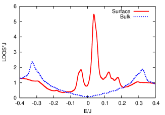
Figure 3: (Color online) LDOS at the surface and in the bulk for $\delta=0.10$.

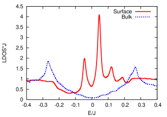
Figure 4: (Color online) LDOS at the surface and in the bulk for $\delta=0.15$.

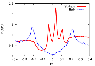
Figure 5: (Color online) LDOS at the surface and in the bulk for $\delta=0.20$.

In order to understand the physical origin of the peak splitting in this model, we show the LDOS at the surface of a state with only $d$-wave SC order, and that with a surface flux phase as well as bulk $d$-wave SC order (i.e., without $s$-wave SCOP) in Fig.6. Here the parameters are the same as those used in Fig.3. It is seen that the peak splitting occurs as long as the flux phase is present. This indicates that the flux-phase order, not the second SCOP Im$\Delta_{s}$, is the necessary ingredient for the peak splitting. We note that it is not possible to have a state with an $s$-wave SCOP without the flux phase in the present model. Next we show the LDOS of a state with bulk (metastable) flux-phase order (type B) in Fig.7. All SCOPs are set to be zero, and the parameters are the same as in Fig.3. The LDOS in the bulk has broad peaks, and one of the peaks shifts near to $E=0$ at the surface. By comparing Figs. 6 and 7 with Fig.3, we can see that the peak structure of the latter is mainly due to the flux phase, and the $d$-wave SC order also contributes to the behavior of the LDOS.

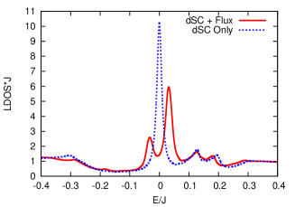
Figure 6: (Color online) LDOS at the surface of a state without $s$-wave SCOP for $\delta=0.10$.

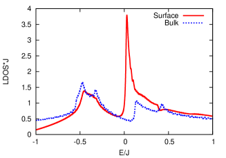
Figure 7: (Color online) LDOS at the surface and in the bulk for a flux phase with $\delta=0.10$. Here all SCOPs are set to be zero

4 Summary

We have studied the states near the (110) surface of high-$T_{C}$ cuprate YBCO that are described by the bilayer $t-J$ model. Near the surface, superconductivity is strongly suppressed, and the flux phase in which the directions of the flux in two layers are opposite may occur in a wide doping region. Then ${\cal T}$ symmetry is violated and the LDOS at the surface has split peaks consistent with experimental findings.[1] The spontaneous magnetic field that could arise near the surface with ${\cal T}$ violation will be very small, because the contributions from two layers essentially cancel out each other. These results may explain why no magnetic field is observed in some experiments for (110) surfaces of YBCO, for which the sign of ${\cal T}$ violation is detected.

The author thanks M. Hayashi and H. Yamase for useful discussions. This work was supported by JSPS KAKENHI Grant Number 24540392.

References

- [1] M. Covington, M. Aprili, E. Paraoanu, L. H. Greene, F. Xu, J. Zhu, and C. A. Mirkin, Phys. Rev. Lett. 79, 277 (1997).
- [2] J. Xia, E. Schemm, G. Deutscher, S. A. Kivelson, D. A. Bonn, W. N. Hardy, R. Liang, W. Siemons, G. Koster, M. M. Fejer, and A. Kapitulnik, Phys. Rev. Lett. 100, 127002 (2008).
- [3] H. Karapetyan, M. Hücker, G. D. Gu, J. M. Tranquada, M. M. Fejer, J. Xia, and A. Kapitulnik, Phys. Rev. Lett. 109, 147001 (2012).
- [4] H. Karapetyan, J. Xia, M. Hucker, G. D. Gu, J. M. Tranquada, M.M. Fejer, A. Kapitulnik, Phys. Rev. Lett. 112, 047003 (2014).
- [5] M. Fogelström, D. Rainer, and J. A. Sauls, Phys. Rev. Lett. 79, 281 (1997).
- [6] M. Matsumoto and H. Shiba, J. Phys. Soc. Jpn. 64, 3384 (1995).
- [7] M. Matsumoto and H. Shiba, J. Phys. Soc. Jpn. 64, 4867 (1995).
- [8] R. Carmi, E. Polturak, G. Koren, and A. Auerbach, Nature 404, 853 (2000).
- [9] H. Saadaoui, Z. Salman, T. Prokscha, A. Suter, H. Huhtinen, P. Paturi, and E. Morenzoni, Phys. Rev. B88, 180501(R) (2013).
- [10] K. Kuboki, J. Phys. Soc. Jpn. 83, 015003 (2014).
- [11] K. Kuboki, J. Phys. Soc. Jpn. 83, 054703 (2014).
- [12] I. Affleck and J. B. Marston, Phys. Rev. B37, 3774 (1988).
- [13] F. C. Zhang, Phys. Rev. Lett. 64, 974 (1990).
- [14] K. Hamada and D. Yoshioka, Phys. Rev. B67, 184503 (2003).
- [15] M. Bejas, A. Greco, and H. Yamase, Phys. Rev. B86, 224509 (2012).
- [16] H. Zhao and J. R. Engelbrecht, Phys. Rev. B 71, 054508 (2005).
- [17] K. Kuboki, J. Phys. Soc. Jpn. 83, 125001 (2014).
- [18] P. G. de Gennes, Superconductivity of Metals and Alloys (Addison-Wesley, Reading, MA, 1989).
- [19] For a review on the model, see M. Ogata and H. Fukuyama, Rep. Prog. Phys. 71, 036501 (2008).
- [20] O. K. Andersen, A. I. Lichtenstein, O. Jepsen, and F. Paulsen, J. Phys. Chem. Solids 56, 1573 (1995).
- [21] Z. Zou and P. W. Anderson, Phys. Rev. B37, 627 (1988).
- [22] P. A. Lee, N. Nagaosa, and X.-G. Wen, Rev. Mod. Phys. 78, 17 (2006).
- [23] G. Kotliar and J. Liu, Phys. Rev. B 38, 5142 (1988).
- [24] Y. Suzumura, Y. Hasegawa, and H. Fukuyama, J. Phys. Soc. Jpn. 57, 2768 (1988).
- [25] F. C. Zhang, C. Gros, T. M. Rice, and H. Shiba, Supercond. Sci. Technol. 1, 36 (1988).
- [26] K. Kuboki, J. Phys. Soc. Jpn. 68, 3150 (1999).
- [27] Y. Tanuma, Y. Tanaka, M. Ogata, and S. Kashiwaya, Phys. Rev. B 60, 9817 (1999).
- [28] J. X. Zhu and C. S. Ting, Phys. Rev. B 61, 1456 (2000).
- [29] K. Kuboki and H. Takahashi, Phys. Rev. B 70, 214524 (2004).
- [30] H. Yamase and W. Metzner, Phys. Rev. B73, 214517 (2006).