Describing many-body bosonic waveguide scattering with the truncated Wigner method

Abstract

We consider quasi-stationary scattering of interacting bosonic matter waves in one-dimensional waveguides, as they arise in guided atom lasers. We show how the truncated Wigner (tW) method, which corresponds to the semiclassical description of the bosonic many-body system on the level of the diagonal approximation, can be utilized in order to describe such many-body bosonic scattering processes. Special emphasis is put on the discretization of space at the exact quantum level, in order to properly implement the semiclassical approximation and the tW method, as well as on the discussion of the results to be obtained in the continuous limit.

I Introduction

The perspective to realize atomtronic devices MicO04PRL ; SeaO07PRA ; PepO09PRL as well as the exploration of transport features that are known from electronic mesoscopic systems BraO12S ; BraO13S have strongly stimulated the research on the dynamical properties of ultracold atoms in open systems. While fermionic atoms provide direct analogies with the electronic case BraO12S ; BraO13S ; BruBel12PRA ; KriO13PRL , the use of a bosonic atomic species brings along new aspects and challenges for the atomic transport problem GutGefMir12PRB ; Iva13EPJB , related, in particular, with the link between a mesoscopic Bose-Einstein condensate in a reservoir and the microscopic dynamics of an ensemble of few interacting atoms within a transistor-like device. A particularly promising configuration for the experimental study of these aspects is provided by the guided atom laser GueO06PRL ; CouO08EPL ; GatO11PRL in which atoms are coherently outcoupled from a trapped Bose-Einstein condensate into an optical waveguide. A coherent atomic beam can thereby be created and injected onto engineered optical scattering geometries. This would allow one to study bosonic many-body scattering at well-defined incident energy.

A theoretical modeling of such waveguide scattering processes within guided atom lasers faces the challenge of dealing with an open system in a many-body context, potentially involving a very large number of atoms in total. Exact diagonalization methods therefore quickly encounter limitations when describing such processes. The Gross-Pitaevskii approximation, on the other hand, which has been used in a number of studies on guided atom laser processes LebPav01PRA ; Car01PRA ; PauRicSch05PRL ; PauO05PRA ; PauO07PRA , is granted to work in the mean-field limit of large atom densities and vanishing atom-atom interaction strengths LieSeiYng00PRA . It is, however, known to break down in the presence of significantly strong interaction effects ErnPauSch10PRA .

The truncated Wigner (tW) method GarZol ; SteO98PRA ; SinLobCas02JPB ; Pol10AP appears to be a reasonable compromise in this context. According to common understanding, this method essentially consists in representing the time evolution of a bosonic many-body quantum state by classical fields evolving according to a Gross-Pitaevskii equation, whose initial values are chosen such that they properly sample the initial quantum state under consideration. They thereby provide a stochastic sampling of the approximated time evolution of the many-body Wigner function defined in the phase space of the bosonic field. The tW method has been successfully applied in a number of contexts involving dynamical processes of ultracold bosonic atoms. This includes, most recently, scattering of atom laser beams within one-dimensional Bose-Hubbard systems DujArgSch15PRA . In this latter transport context, the tW method was shown to yield quantitative predictions for the average transmitted current that were shown to be in good agreement with complementary matrix-product state calculations in the regime of moderate on-site interaction strenghts DujArgSch15PRA .

While it is possible to formulate the tW method in a functional manner OpaDru13JMP , its practical implementation is most conveniently achieved by means of a discrete basis of the single-particle Hilbert space. This is straightforward to accomplish for dynamical process that are effectively taking place within spatially confined regions. In that case, periodic boundary conditions can, e.g., be imposed at a sufficiently large distance from the quantum many-body wave packet to be studied, giving thereby rise to an effective discretization in momentum space. This is, however, not a viable option for studying quasi-stationary scattering processes which are generally characterized by an infinite spatial extension. We therefore propose to discretize the position space in order to implement the tW method in this context, as was effectively done in Ref. DujArgSch15PRA A primary purpose of this paper is to introduce this discretization procedure in some detail and discuss its validity in the continuous limit, both from an analytical and from a numerical point of view.

Moreover, we present in this paper an unconventional derivation of the tW method in the framework of the semiclassical van Vleck-Gutzwiller theory Gut . This allows us to identify the tW method with the diagonal semiclassical approximation in the bosonic field-theoretical context, and, as shown in Ref. EngO14PRL , to quantitatively account for interference effects beyond tW. We note that the tW method can also be derived through other approaches such as Wigner-Moyal expansions SteO98PRA ; SinLobCas02JPB ; Pol10AP , quasiclasical corrections to the effective action Pol03PRA , and the so-called semiclassical approximation in the context of the Keldysh approach Kam . In those approaches, however, quantum corrections are perturbatively incorporated on top of a classical background given by the propagation of phase space distributions along classical trajectories that are accounted for in an independent (i.e. incoherent) manner. Interference effects involving different trajectories are essentially non-perturbative and require special resummation techniques that are justified only in the presence of small parameters, (typically the strength of interactions or the size of quantum fluctuations). While the van Vleck-Gutzwiller theory yields exactly the same (tW) approximation to leading (classical) order as the other approaches mentioned above, its key asset resides in the fact that it can readily incorporate quantum interference in a non-perturbative manner and describe, e.g., coherent backscattering in the Fock space of many-body systems EngO14PRL . This is our primary long-term motivation to advertise this approach in this article.

Our paper is organized as follows: In Section II we shall discuss in some detail the spatial discretization procedure of one-dimensional waveguide scattering configurations. Section III is devoted to deriving the tW method in the framework of the van Vleck-Gutzwiller theory. We shall then argue in Section IV.1 that the tW approach can be reformulated in terms of a stochastic Gross-Pitaevskii equation whose noisy components exhibit well-defined statistical characteristics in the continuous limit. These findings are confirmed by numerical results on transport through a symmetric double barrier potential, as we show in Section IV.2: Both the average total current of atoms and its incoherent part tend to finite values in the continuous limit.

II Discretization of space

We consider a many-body scattering process of a coherent atomic matter-wave beam within a waveguide. This matter-wave beam is supposed to be created by a coherent outcoupling process from a trapped Bose-Einstein condensate, as is commonly done in guided atom lasers GueO06PRL ; CouO08EPL ; GatO11PRL . If we assume that only the transverse ground mode of the waveguide is populated, we can describe this system by the many-body Hamiltonian

$$\hat{H} = \int_{-\infty}^{\infty}\hat{\psi}^{\dagger}(x)\left(-\frac{\hbar^{2}}{2m}\frac{\partial^{2}}{\partial x^{2}}+V(x)\right)\hat{\psi}(x)dx$$ (1)

$$+\frac{1}{2}\int_{-\infty}^{\infty}g(x)\hat{\psi}^{\dagger}(x)\hat{\psi}^{\dagger}(x)\hat{\psi}(x)\hat{\psi}(x)dx$$

$$+\int_{-\infty}^{\infty}\kappa(x)\left(\hat{\psi}^{\dagger}(x)\hat{b}+\hat{b}^{\dagger}\hat{\psi}(x)\right)dx+\mu\hat{b}^{\dagger}\hat{b}$$

where $\hat{\psi}^{\dagger}(x)$ and $\hat{\psi}(x)$ respectively represent the creation and annihilation operators of a bosonic particle at the longitudinal position $x$ within the waveguide. $m$ is the mass of the atoms, $V(x)$ describes a scattering potential (given, e.g., by a sequence of barriers) within the waveguide, and $g(x)$ is the spatially dependent one-dimensional interaction strength of the atoms in the waveguide. It is approximately given by $g(x)\simeq 2\hbar\omega_{\perp}(x)a_{s}(x)$ Ols98PRL where $\omega_{\perp}$ is the transverse confinement frequency of the waveguide and $a_{s}$ is the (generally very small) s-wave scattering length of the atomic species under consideration. Both $\omega_{\perp}$ and $a_{s}$ can depend on the position in the waveguide, the former through a spatial variation of the transverse confinement, and the latter through a spatially dependent Feshbach tuning.

The trap is modeled by a single one-particle state with energy $\mu$ whose associated creation an annihilation operators are given by $\hat{b}^{\dagger}$ and $\hat{b}$. Trapped atoms are outcoupled to the waveguide through the spatially dependent (real) coupling strength $\kappa(x)$, which, e.g., in Ref. GueO06PRL would model the effect of a radiofrequency field that flips the spin of the atoms. We shall in the following assume a macroscopically large initial population $N\to\infty$ of the atoms in the trap in combination with a very small outcoupling strength $\kappa\to 0$, such that the trapped condensate is not appreciably affected by the outcoupling process on finite evolution times. The time evolution of the system can then be effectively described by the equation

$$i\hbar\frac{\partial}{\partial t}\hat{\psi}(x,t) = \left(-\frac{\hbar^{2}}{2m}\frac{\partial^{2}}{\partial x^{2}}+V(x)-\mu\right)\hat{\psi}(x,t)+\kappa(x)\hat{b}e^{-i\mu t/\hbar}$$ (2)

$$+g(x)\hat{\psi}^{\dagger}(x,t)\hat{\psi}(x,t)\hat{\psi}(x,t)$$

for the time-dependent field operator $\hat{\psi}(x,t)$ describing atoms in the waveguide.

In order to implement the tW method for this many-body scattering problem, we first need to introduce a discretization procedure of this spatially continuous quantum field equation. As pointed out above, such a discretization cannot be defined in momentum or energy space (e.g. through the introduction of periodic boundary conditions at $x=\pm L$ for some large $L\to\infty$) as this would not be compatible with the formation of a quasi-stationary scattering state. We therefore propose to discretize the position space, namely through the introduction of a high-energy cutoff in momentum space at $p=\pm\pi\hbar/\delta$ for some effective spatial grid size $\delta\to 0$. Correspondingly, we also modify the Hamiltonian of the free kinetic energy close to the high-energy cutoff, such that it reads

$$\hat{H}_{0}=E_{\delta}\int_{-\infty}^{\infty}\hat{\psi}^{\dagger}(x)\left(1-\cos(\delta\hat{p}/\hbar)\right)\hat{\psi}(x)dx$$ (3)

with $E_{\delta}=\hbar^{2}/(m\delta^{2})$ and $\hat{p}=-i\hbar\partial/\partial x$. This Hamiltonian is still diagonalized in the eigenbasis of the normalized waves $\tilde{\phi}_{k}(x)=\exp(ikx)/\sqrt{2\pi}$ satisfying $\int_{-\infty}^{\infty}\tilde{\phi}_{k}^{*}(x)\tilde{\phi}_{k^{\prime}}(x)dx=\delta(k-k^{\prime})$. Their associated eigenvalues now read $E_{k}=E_{\delta}(1-\cos k\delta)$ close to the cutoff while they are still approximately given by $E_{k}\simeq\hbar^{2}k^{2}/(2m)$ for $k\delta\ll 1$.

In close analogy with the theory of spatially periodic systems, we now introduce an effective Wannier basis through the spatially localized functions

$$\phi_{l}(x) = \sqrt{\frac{\delta}{2\pi}}\int_{-\pi/\delta}^{\pi/\delta}\tilde{\phi}_{k}(x)e^{-ilk\delta}dk$$ (4)

$$= \frac{1}{\sqrt{\delta}}\mathrm{sinc}\left(\frac{\pi}{\delta}(x-l\delta)\right)$$ (5)

for integer $l\in\mathbb{Z}$, with $\mathrm{sinc}(x)\equiv\sin(x)/x$, which can effectively be seen as Fourier series coefficients of the waves $\tilde{\phi}_{k}$. They therefore satisfy $\int_{-\infty}^{\infty}\phi_{l}^{*}(x)\phi_{l^{\prime}}(x)dx=\delta_{ll^{\prime}}$ and thereby form an orthogonal basis set that spans the restricted Hilbert space obtained after the introduction of the momentum cutoff. Defining the corresponding creation and annihilation operators $\hat{\psi}_{l}^{\dagger}$, $\hat{\psi}_{l}$ such that we have $\hat{\psi}(x)=\sum_{l=-\infty}^{\infty}\phi_{l}(x)\hat{\psi}_{l}$, we can now reformulate the free kinetic Hamiltonian (3) such that it reads

$$\hat{H}_{0}=\frac{1}{2}E_{\delta}\sum_{l=-\infty}^{\infty}\left(2\hat{\psi}_{l}^{\dagger}\hat{\psi}_{l}-\hat{\psi}_{l+1}^{\dagger}\hat{\psi}_{l}-\hat{\psi}_{l}^{\dagger}\hat{\psi}_{l+1}\right)\,.$$ (6)

This expression is identical to the one that would be obtained from a finite-difference approximation of the kinetic energy in the waveguide.

Altogether, we thereby obtain in the limit $\delta\to 0$ the effective Bose-Hubbard Hamiltonian

$$\hat{H} = \sum_{l=-\infty}^{\infty}\left[(E_{\delta}-\mu+V_{l})\hat{\psi}_{l}^{\dagger}\hat{\psi}_{l}-\frac{E_{\delta}}{2}\left(\hat{\psi}_{l+1}^{\dagger}\hat{\psi}_{l}+\hat{\psi}_{l}^{\dagger}\hat{\psi}_{l+1}\right)\right.$$ (7)

$$\left.+\frac{g_{l}}{2}\hat{\psi}_{l}^{\dagger}\hat{\psi}_{l}^{\dagger}\hat{\psi}_{l}\hat{\psi}_{l}+\kappa_{l}\left(\hat{\psi}_{l}^{\dagger}\hat{b}+\hat{b}^{\dagger}\hat{\psi}_{l}\right)\right]$$

where we introduce the definitions $V_{l}\equiv V(l\delta)$, $g_{l}\equiv g(l\delta)/\delta$, and $\kappa_{l}\equiv\sqrt{\delta}\kappa(l\delta)$, and where, for the sake of convenience, we redefine in Eq. (7) the zero of the energy scale such that it coincides with the energy of trapped atoms. The time evolution of the discrete field operator $\hat{\psi}_{l}$ is then given by

$$i\hbar\frac{\partial}{\partial t}\hat{\psi}_{l}(t) = (E_{\delta}-\mu+V_{l})\hat{\psi}_{l}(t)-\frac{E_{\delta}}{2}\left(\hat{\psi}_{l-1}(t)+\hat{\psi}_{l+1}(t)\right)$$ (8)

$$+g_{l}\hat{\psi}_{l}^{\dagger}(t)\hat{\psi}_{l}(t)\hat{\psi}_{l}(t)+\kappa_{l}\hat{b}\,.$$

III Semiclassical derivation of the truncated Wigner method

Having accomplished the discretization of the exact quantum description, a semiclassical approach can be used in the regime of large particle numbers $N\gg 1$, which does not resort to the numerical solution of the operator-valued equations (8). This approach has three levels of approximation. The first level is the purely classical limit consisting of the propagation of the (discretized) Gross-Pitaevskii equation that is obtained from Eq. (8) by the substitution $\hat{\psi}_{l}(t)\mapsto\psi_{l}(t)$ and $\hat{\psi}_{l}^{\dagger}(t)\mapsto\psi_{l}^{*}(t)$ where the latter classical fields are canonically conjugated variables. In a second step, a finite initial phase-space distribution of the quantum many-body Wigner function is accounted for. This phase-space distribution can contain non-classical correlations which is, however, not the case in our present problem. Finally, a full-fledged semiclassical approximation is obtained by coherently adding amplitudes associated with classical trajectories, in order to address quantum interference effects SimStr14PRA . The second stage in this hierarchy of levels of approximation is the tW method. Here we derive this method in an unconventional manner which is based on a semiclassical approximation of the Feynman propagator of our effective Bose-Hubbard system (7) in terms of a coherent sum over solutions of the mean-field equations.

The notion of the term ”semiclassical” in our approach is conceptually different from its meaning in the context of the Moyal-Wigner expansion used in quantum optics SteO98PRA ; SinLobCas02JPB ; Pol10AP , the quantum corrections to the effective action of Ref. Pol03PRA , and the quasiclassical corrections within the Keldysh approach Kam . In those approaches, the classical limit is identified in terms of the transport equations of probability distributions in phase space (the so-called classical field in the Keldysh language Kam ), while quantum corrections are systematically incorporated as perturbation series around this classical background. Although interference effects, with their charateristic non-perturbative dependence on $\hbar$, can be obtained within those frameworks by special resummation techniques, these techniques are in principle not suitable to tackle classically chaotic situations where all relevant physical forces governing the dynamics of the system under consideration are of the same order and no small parameter can be identified.

The semiclassical van Vleck-Gutzwiller approach, on the other hand, is particularly powerful precisely in this chaotic regime where it allows one to predict universal interference effects. Its key feature is that it approximates the quantum time evolution of the system by a semiclassical superposition of amplitudes and therefore explicitly accounts for quantum mechanical interference through coherent double sums over classical paths. By working with amplitudes instead of probabilities, we can explicitely identify tW with the assumption that pairs of different classical solutions have uncorrelated actions. Going beyond this so-called diagonal approximation and taking into account systematic off-diagonal contributions, the semiclassical approach has been used to predict interference effects beyond both tW and its quasiclassical corrections in good agreeement with numerical simulations EngO14PRL ; EngUrbRic14xxx .

Following Ref. EngO14PRL , we begin with the time evolution of an arbitrary many body state, $|\Psi(t)\rangle=\hat{U}(t)|\Psi(0)\rangle$, governed by the time evolution operator $\hat{U}(t)=\exp(-it\hat{H}/\hbar)$ associated with the Hamiltonian (7). Our Hilbert space

$${\cal H}=\mathrm{span}\{|{\mathbb{n}}\rangle\equiv|\ldots,n_{-1},n_{0},n_{1},\ldots\rangle,n_{l}\in\mathbb{N}_{0}\}$$ (9)

is spanned by the Fock states associated with the site basis, where the discretized field operators act in the usual manner, namely by raising or lowering the number of particles in a given site:

$$\hat{\psi}_{l}^{\dagger}|\ldots,n_{l},\ldots\rangle = \sqrt{n_{l}+1}|\ldots,n_{l}+1,\ldots\rangle\,,$$ (10)

$$\hat{\psi}_{l}|\ldots,n_{l},\ldots\rangle = \sqrt{n_{l}}|\ldots,n_{l}-1,\ldots\rangle\,.$$ (11)

The starting point of our approach is to use of a different basis for ${\cal H}$, which is the formal equivalent of the position representation used in the usual derivation of the Feynman propagator in first-quantized systems. This new basis $|{\mathbb{q}}\rangle$ is given by the common eigenstates of the commuting set of hermitian operators $\hat{q}_{l}=\sqrt{\hbar/2}(\hat{\psi}_{l}+\hat{\psi}_{l}^{\dagger})$ which are known in quantum optics as quadratures. Using the defining property $\hat{q}_{l}|{\mathbb{q}}\rangle=q_{l}|{\mathbb{q}}\rangle$, the orthonormality and completness relations $\langle{\mathbb{q}}|{\mathbb{q}}^{\prime}\rangle=\delta({\mathbb{q}}-{\mathbb{q}}^{\prime})$ and $\int d{\mathbb{q}}|{\mathbb{q}}\rangle\langle{\mathbb{q}}|=\hat{1}$ of the quadrature basis follow directly.

Having at hand a complete basis with continuous states, a path integral representation of the time evolution operator can be obtained in the usual way. Contrary to the usual kinetic-plus-potential Hamiltonian in the first-quantized case, the use of the eigenstates $|{\mathbb{p}}\rangle$ of the momentum quadratures $\hat{p}_{l}=-i\sqrt{\hbar/2}(\hat{\psi}_{l}-\hat{\psi}_{l}^{\dagger})$ is not only useful but essential to get the amplitude $K({\mathbb{q}}^{\rm f},{\mathbb{q}}^{\rm i},t)\equiv\langle{\mathbb{q}}^{\rm f}|\hat{U}(t)|{\mathbb{q}}^{\rm i}\rangle$ of the propagation from an initial to a final quadrature state

$$K({\mathbb{q}}^{\rm f},{\mathbb{q}}^{\rm i},t)=\int{\cal D}[{\mathbb{q}}(s),{\mathbb{p}}(s)]{\rm e}^{iR[{\mathbb{q}}(s),{\mathbb{p}}(s)]/\hbar}$$ (12)

in the form of an integral over paths ${\mathbb{q}}(s),{\mathbb{p}}(s)$ satisfying the boundary (shooting) conditions ${\mathbb{q}}(s=0)={\mathbb{q}}^{\rm i}$ and ${\mathbb{q}}(s=t)={\mathbb{q}}^{\rm f}$. Here, the action functional is given in its Hamiltonian form,

$$R[{\mathbb{q}}(s),{\mathbb{p}}(s)]=\int_{0}^{t}ds[\dot{{\mathbb{q}}}(s)\cdot{\mathbb{p}}(s)-H^{\rm cl}({\mathbb{q}}(s),{\mathbb{p}}(s))]$$ (13)

where the classical Hamiltonian $H^{\rm cl}$ is obtained from the quantum one by the substitutions $\hat{\psi}_{l}\mapsto\psi_{l}$ and $\hat{\psi}_{l}^{\dagger}\mapsto\psi_{l}^{*}$ with $\psi_{l}\equiv(q_{l}+ip_{l})/\sqrt{2\hbar}$. Properly taking care of the Weyl ordering of operators, which yields the replacement $\hat{\psi}_{l}\hat{\psi}_{l}^{\dagger}+\hat{\psi}_{l}^{\dagger}\hat{\psi}_{l}\mapsto 2\psi_{l}^{*}\psi_{l}$, we then obtain from Eq. (7) the classical Gross-Pitaevskii-type Hamiltonian

$$H^{\rm cl} = \sum_{l=-\infty}^{\infty}\left[(E_{\delta}-\mu+V_{l})\psi_{l}^{*}\psi_{l}-\frac{E_{\delta}}{2}\left(\psi_{l+1}^{*}\psi_{l}+\psi_{l}^{*}\psi_{l+1}\right)\right.$$ (14)

$$\left.+\frac{g_{l}}{2}\psi_{l}^{*}\psi_{l}(\psi_{l}^{*}\psi_{l}-2)+\kappa_{l}\left(\psi_{l}^{*}b+b^{*}\psi_{l}\right)\right]$$

up to constant terms that are not important.

We now continue with a stationary phase analysis of the path integral, following Gutzwiller’s pionering work in the 60’s and 70’s Gut . This programme was accomplished in Ref. EngO14PRL . It yields as final result the propagator

$$K({\mathbb{q}}^{\rm f},{\mathbb{q}}^{\rm i},t)\simeq\sum_{\gamma}\left|{\rm det}\frac{\partial^{2}}{\partial{\mathbb{q}}^{\rm i}\partial{\mathbb{q}}^{\rm f}}\frac{R_{\gamma}({\mathbb{q}}^{\rm f},{\mathbb{q}}^{\rm i},t)}{2\pi\hbar}\right|^{1/2}{\rm e}^{iR_{\gamma}({\mathbb{q}}^{\rm f},{\mathbb{q}}^{\rm i},t)/\hbar}$$ (15)

as a sum over all solutions of the classical shooting problem (up to an extra phase $i\mu_{\gamma}\pi/4$ involving the Maslov index $\mu_{\gamma}$, which is not important in the following).

The time evolution of the expectation value $\langle\hat{A}\rangle_{t}\equiv\langle\Psi(t)|A(\hat{\mathbb{q}},\hat{\mathbb{p}})|\Psi(t)\rangle$ of a properly (Weyl) ordered operator $\hat{A}=A(\hat{\mathbb{q}},\hat{\mathbb{p}})$ is given by

$$\langle\hat{A}\rangle_{t} = \int d{\mathbb{q}}^{\rm f}d{\mathbb{q}}^{\rm i}d{\mathbb{q}^{\prime}}^{\rm i}\langle{\mathbb{q}^{\prime}}^{\rm i}|\Psi(0)\rangle\langle\Psi(0)|{\mathbb{q}}^{\rm i}\rangle$$ (16)

$$\times K({\mathbb{q}}^{\rm f},{\mathbb{q}}^{\rm i},t)^{*}A({\mathbb{q}}^{\rm f},-i\hbar\partial/\partial{\mathbb{q}}^{\rm f})K({\mathbb{q}}^{\rm f},{\mathbb{q}^{\prime}}^{\rm i},t).$$

Our goal is to obtain a semiclassical approximation for this expression. As first step, we substitute the semiclassical propagator (15) in Eq. (16). At this level of approximation, we only assume that a typical action in Eq. (13) is significantly larger than $\hbar$. In that limit, for any smooth functions $F(x),G(x),H(x)$ we have

$$F\left(-i\hbar\frac{\partial}{\partial{\mathbb{q}}}\right)G({\mathbb{q}}){\rm e}^{\frac{iH({\mathbb{q}})}{\hbar}}=F\left(\frac{\partial H({\mathbb{q}})}{\partial{\mathbb{q}}}\right)G({\mathbb{q}}){\rm e}^{\frac{iH({\mathbb{q}})}{\hbar}}+{\cal O}(\hbar).$$ (17)

Using $\partial R_{\gamma}({\mathbb{q}}^{\rm f},{\mathbb{q}^{\prime}}^{\rm i},t)/\partial{\mathbb{q}}^{\rm f}={\mathbb{p}}^{\rm f}_{\gamma}({\mathbb{q}}^{\rm f},{\mathbb{q}}^{\rm i},t)$, we obtain then

$$A({\mathbb{q}}^{\rm f},-i\hbar\partial/\partial{\mathbb{q}}^{\rm f})K({\mathbb{q}}^{\rm f},{\mathbb{q}^{\prime}}^{\rm i},t)$$ (18)

$$\simeq \sum_{\gamma}A({\mathbb{q}}^{\rm f},{\mathbb{p}}_{\gamma}^{\rm f})\left|{\rm det}\frac{\partial^{2}}{\partial{\mathbb{q}}^{\rm i}\partial{\mathbb{q}}^{\rm f}}\frac{R_{\gamma}({\mathbb{q}}^{\rm f},{\mathbb{q}}^{\rm i},t)}{2\pi\hbar}\right|^{1/2}{\rm e}^{iR_{\gamma}({\mathbb{q}}^{\rm f},{\mathbb{q}}^{\rm i},t)/\hbar}.$$

This then yields a double sum over classical trajectories in Eq. (16). It is remarkably accurate even for moderate values of the classical actions and for arbitrary large times, and it sucessfully describes interference phenomena through the coherent sum over the oscillatory amplitudes that are associated with each trajectory.

In a further approximation, one makes use of the fact that the double sum over paths contains a large number of terms that effectively cancel each other in the presence of an average over initial and final positions as in Eq. (16). Only pairs of trajectories with similar actions yield nonvanishing contributions due to phase cancellations, which gives rise to incoherent sums of slowly oscillatory terms with non-zero average. This is the essence of the diagonal approximation, the standard tool to obtain leading, classical-like, contributions from coherent double sums representing semiclassical amplitudes. In the present context, the diagonal approximation is implemented by pairing $\gamma({\mathbb{q}}^{\rm f},{\mathbb{q}}^{\rm i},t)$ and $\gamma({\mathbb{q}}^{\rm f},{\mathbb{q}^{\prime}}^{\rm i},t)$ for which ${\mathbb{q}}^{\rm i}\simeq{\mathbb{q}^{\prime}}^{\rm i}$. In the semiclassical limit, all smooth terms in the propagator are then evaluated at ${\mathbb{q}}=({\mathbb{q}}^{\rm i}+{\mathbb{q}^{\prime}}^{\rm i})/2$, while the actions are expanded up to first order in ${\mathbb{q}}^{\rm i}-{\mathbb{q}^{\prime}}^{\rm i}$ according to $R_{\gamma}({\mathbb{q}}^{\rm f},{\mathbb{q}}^{\rm i},t)-R_{\gamma}({\mathbb{q}}^{\rm f},{\mathbb{q}^{\prime}}^{\rm i},t)\simeq-{\mathbb{p}}_{\gamma}^{\rm i}({\mathbb{q}}^{\rm f},{\mathbb{q}},t)\cdot({\mathbb{q}}^{\rm i}-{\mathbb{q}^{\prime}}^{\rm i})$.

The double sums are then transformed into a single sum yielding the diagonal approximation for $\langle\hat{A}\rangle_{t}$ as

$$\langle\hat{A}\rangle_{t}^{\rm d} = \int d{\mathbb{q}}^{\rm f}d{\mathbb{q}}^{\rm i}d{\mathbb{q}^{\prime}}^{\rm i}\langle{\mathbb{q}^{\prime}}^{\rm i}|\Psi(0)\rangle\langle\Psi(0)|{\mathbb{q}}^{\rm i}\rangle\sum_{\gamma}A[{\mathbb{q}}^{\rm f},{\mathbb{p}}_{\gamma}^{\rm f}({\mathbb{q}}^{\rm f},{\mathbb{q}},t)]$$ (19)

$$\times \left|{\rm det}\frac{\partial^{2}}{\partial{\mathbb{q}}\partial{\mathbb{q}}^{\rm f}}\frac{R_{\gamma}({\mathbb{q}}^{\rm f},{\mathbb{q}},t)}{2\pi\hbar}\right|{\rm e}^{-i{\mathbb{p}}_{\gamma}^{\rm i}({\mathbb{q}}^{\rm f},{\mathbb{q}},t)\cdot({\mathbb{q}}^{\rm i}-{\mathbb{q}^{\prime}}^{\rm i})/\hbar}.$$

This expression can be further simplified by noticing that $\partial^{2}R_{\gamma}({\mathbb{q}}^{\rm f},{\mathbb{q}},t)/\partial{\mathbb{q}}\partial{\mathbb{q}}^{\rm f}=-\partial{\mathbb{p}}^{\rm i}_{\gamma}({\mathbb{q}}^{\rm f},{\mathbb{q}},t)/\partial{\mathbb{q}}^{\rm f}$ is the Jacobian matrix of the transformation ${\mathbb{q}}^{\rm f}\to{\mathbb{p}}^{\rm i}$, as these variables are functionally dependent through the solutions ${\mathbb{q}}^{\rm f}={\mathbb{q}}^{\rm f}({\mathbb{q}},{\mathbb{p}}^{\rm i},t)$, ${\mathbb{p}}^{\rm f}={\mathbb{p}}^{\rm f}({\mathbb{q}},{\mathbb{p}}^{\rm i},t)$ of the classical equations of motion. We can then change the integration over final coordinates by an integration over initial momenta. Together with the substitution $({\mathbb{q}}^{\rm i},{\mathbb{q}^{\prime}}^{\rm i})\mapsto({\mathbb{q}},{\mathbb{x}})$ with ${\mathbb{q}}=({\mathbb{q}}^{\rm i}+{\mathbb{q}^{\prime}}^{\rm i})/2$ and ${\mathbb{x}}={\mathbb{q}}^{\rm i}-{\mathbb{q}^{\prime}}^{\rm i}$ (and with the replacement ${\mathbb{p}}^{\rm i}\equiv{\mathbb{p}}$), this finally yields

$$\langle\hat{A}\rangle_{t}^{\rm d}=\int d{\mathbb{q}}d{\mathbb{p}}A[{\mathbb{q}}^{\rm f}({\mathbb{q}},{\mathbb{p}},t),{\mathbb{p}}^{\rm f}({\mathbb{q}},{\mathbb{p}},t)]W_{\Psi(0)}({\mathbb{q}},{\mathbb{p}}),$$ (20)

where we introduce the Wigner function associated with the state $|\Phi\rangle$ through

$$W_{\Phi}({\mathbb{q}},{\mathbb{p}})=\left(\prod_{l}\int\frac{dx_{l}}{2\pi\hbar}\right){\rm e}^{-i{\mathbb{p}}\cdot{\mathbb{x}}/\hbar}\langle{\mathbb{q}}+{\mathbb{x}}/2|\Phi\rangle\langle\Phi|{\mathbb{q}}-{\mathbb{x}}/2\rangle$$ (21)

with the product $\prod_{l}$ going over all single-particle sites rem_exact . It is possible to reformulate Eq. (20) as

$$\langle\hat{A}\rangle_{t}^{\rm d}=\int d{\mathbb{q}}d{\mathbb{p}}A({\mathbb{q}},{\mathbb{p}})W_{\Psi(0)}({\mathbb{q}},{\mathbb{p}},t)$$ (22)

where $W_{\Psi(0)}({\mathbb{q}},{\mathbb{p}},t)$ is the time-dependent Wigner function which evolves according to the well-known truncated Wigner equation. This demonstrates that the tW method is obtained by neglecting off-diagonal terms in the semiclassical calculation of time-dependent expectation values of quantum observables.

For the waveguide scattering configuration under consideration, the classical field equations to be numerically integrated in the framework of the tW method are derived from Eq. (14) and read

$$i\hbar\frac{\partial}{\partial t}\psi_{l}(t) = (E_{\delta}-\mu+V_{l})\psi_{l}(t)-\frac{E_{\delta}}{2}\left(\psi_{l-1}(t)+\psi_{l+1}(t)\right)$$ (23)

$$+g_{l}\left(|\psi_{l}(t)|^{2}-1\right)\psi_{l}(t)+\sqrt{N}\kappa_{l}\,.$$

Here we represent, in the limit of a large number of atoms $N\to\infty$, the Bose-Einstein condensate in the trap by a coherent state with the amplitude $\sqrt{N}$ and with vanishing relative uncertainty in its amplitude and phase. The initial quantum state in the waveguide, on the other hand, is a vacuum state that has to be correctly sampled in the framework of the truncated Wigner method. More specifically, the initial field amplitudes in the discretized waveguide have to be chosen as $\psi_{l}(0)=(A_{l}+iB_{l})/2$ where $A_{l}$ and $B_{l}$ are independent Gaussian random variables with zero mean and unit variance. As a consequence, each site $l$ of the grid representing the empty waveguide has initially the average classical density

$$\overline{|\psi_{l}(0)|^{2}}=1/2$$ (24)

where the overline denotes the tW average over the random variables. This pseudo-density of half a particle per grid point is to be subtracted when calculating the average atomic density $\rho(x,t)=\langle\hat{\psi}^{\dagger}(x,t)\hat{\psi}(x,t)\rangle$ using the tW method: this average density is evaluated as

$$\rho(x=l\delta,t)=\frac{1}{\delta}\left(\overline{|\psi_{l}(t)|^{2}}-1/2\right)\,.$$ (25)

The current $j(x,t)=\mathrm{Re}[\langle\hat{\psi}^{\dagger}(x,t)\hat{p}\hat{\psi}(x,t)\rangle]/m$, on the other hand, is not articifially affected by the vacuum fluctuations; it is evaluated as

$$j(x=l\delta,t)=\frac{\hbar}{2im\delta^{2}}\left(\overline{\psi_{l}^{*}(t)\psi_{l+1}(t)-\psi_{l+1}^{*}(t)\psi_{l}(t)}\right)\,.$$ (26)

For both the density and the current we can define coherent components according to

$$\rho^{\rm coh}(l\delta,t) = \frac{1}{\delta}\left|\overline{\psi_{l}(t)}\right|^{2}\,,$$ (27)

$$j^{\rm coh}(l\delta,t) = \frac{\hbar}{2im\delta^{2}}\left(\overline{\psi_{l}^{*}(t)}\,\overline{\psi_{l+1}(t)}-\overline{\psi_{l+1}^{*}(t)}\,\overline{\psi_{l}(t)}\right)\,,$$ (28)

which result from a direct tW average of the complex amplitudes $\psi_{l}$. They would correspond to the mean-field predictions obtained by the classical Gross-Pitaevskii approach in the limit of large densities and vanishing atom-atom interaction strength. The associated incoherent components are defined through

$$\rho^{\rm incoh}(l\delta,t) = \rho(l\delta,t)-\rho^{\rm coh}(l\delta,t)\,,$$ (29)

$$j^{\rm incoh}(l\delta,t) = j(l\delta,t)-j^{\rm coh}(l\delta,t)\,.$$ (30)

They approximately characterize the amount of quantum depletion in the waveguide.

IV The continuous limit

IV.1 Quantum noise

The tW method is certified to be valid in the semiclassical regime where the average population per single-particle state is large compared to unity. However, this condition is no longer met in the continuous limit of vanishing grid spacing $\delta\to 0$. Indeed, assuming that the scattering process under consideration gives rise to a well-defined average atom density $\rho(x,t)$ in the waveguide, the corresponding discrete mean-field amplitudes would essentially be given by $\psi_{l}(t)\simeq\sqrt{\delta\rho(l\delta,t)}$. In the limit $\delta\to 0$ they would thereby become negligibly small as compared to the vacuum fluctuations which still feature half a (pseudo-)particle per grid point according to Eq. (24).

The purpose of this section is not to discuss the validity of the tW method in the continuous limit (which would obviously require the comparison of numerical results with a complementary, and genuinely quantum, method, such as exact diagonalization) but to argue that it yields consistent results in this limit. We shall, for this purpose, introduce a Bogoliubov decomposition of the tW amplitude according to $\psi_{l}(t)=\chi_{l}(t)+\varphi_{l}(t)$ where $\chi_{l}$ results from the unperturbed time evolution of the vacuum fluctuation according to

$$i\hbar\frac{\partial}{\partial t}\chi_{l}(t) = (E_{\delta}-\mu+V_{l})\chi_{l}(t)-\frac{E_{\delta}}{2}\left(\chi_{l-1}(t)+\chi_{l+1}(t)\right)$$ (31)

$$+g_{l}\left(|\chi_{l}(t)|^{2}-1\right)\chi_{l}(t)$$

with the initial condition $\chi_{l}(0)=\psi_{l}(0)$. This equation will not change the characteristics of the vacuum fluctuations in the course of time evolution as it obviously corresponds to the truncated Wigner modeling of an empty waveguide. Through Eqs. (23) and (31), $\varphi_{l}\equiv\psi_{l}-\chi_{l}$ then evolves according to

$$i\hbar\frac{\partial}{\partial t}\varphi_{l}(t) = (E_{\delta}-\mu+V_{l})\varphi_{l}(t)-\frac{E_{\delta}}{2}\left(\varphi_{l-1}(t)+\varphi_{l+1}(t)\right)$$ (32)

$$+g_{l}|\varphi_{l}(t)|^{2}\varphi_{l}(t)+\sqrt{N}\kappa_{l}$$

$$+g_{l}\left[(2|\chi_{l}(t)|^{2}-1)\varphi_{l}(t)+\chi_{l}^{2}(t)\varphi_{l}^{*}(t)\right]$$

$$+g_{l}\left[(2\chi_{l}(t)|\varphi_{l}(t)|^{2}+\chi_{l}^{*}(t)\varphi_{l}^{2}(t)\right]\,,$$

which effectively corresponds to a stochastic Gross-Pitaevskii equation. Indeed, the first two lines of Eq. (32) describe the mean-field Gross-Pitaveskii modeling of the waveguide scattering process, with $\varphi_{l}(0)=0$ as initial condition in the waveguide. The other two lines contain quantum noise terms that randomly perturb the evolution of the coherent field $\varphi_{l}$ emitted by the outcoupling process from the trap.

It is instructive to quantitatively evaluate the characteristics of this quantum noise in the continuous limit $\delta\to 0$. In that limit, we can neglect the last line of Eq. (32) since this particular noise term is suppressed to the noise terms in the third line of Eq. (32) by a scaling factor $\sqrt{\delta}$ (noting that $g_{l}\sim 1/\delta$ and $\varphi_{l}\sim\sqrt{\delta}$ for $\delta\to 0$). We can, furthermore, analytically integrate Eq. (31) by neglecting the effect of $\mu$, $V_{l}$ and $g_{l}$ as compared to $E_{\delta}$ (and by using the fact that noise amplitudes $\chi_{l}$ on adjacent grid points are uncorrelated, in striking contrast to the coherent amplitudes $\varphi_{l}$). This yields

$$\chi_{l}(t)=\sum_{l^{\prime}=-\infty}^{\infty}\psi_{l}(0)i^{l-l^{\prime}}J_{l-l^{\prime}}(E_{\delta}t/\hbar)e^{-iE_{\delta}t/\hbar}$$ (33)

where $J_{l}$ denotes the Bessel function of the first kind of the order $l$. We thereby obtain the temporal correlation function of the quantum noise as

$$\overline{\chi_{l}^{*}(t)\chi_{l^{\prime}}(t^{\prime})}=\frac{1}{2}i^{l^{\prime}-l}J_{l^{\prime}-l}\left(E_{\delta}(t^{\prime}-t)/\hbar\right)e^{-iE_{\delta}(t^{\prime}-t)/\hbar}\,,$$ (34)

which reproduces Eq. (24) as special case for $t=t^{\prime}$.

The third line of Eq. (32) can then be rewritten as $\xi_{l}(t)\varphi_{l}(t)+\eta_{l}(t)\varphi_{l}^{*}(t)$ with the effective (real and complex) noise terms

$$\xi_{l}(t) = g_{l}(2|\chi_{l}(t)|^{2}-1)\,,$$ (35)

$$\eta_{l}(t) = g_{l}\chi_{l}^{2}(t)$$ (36)

that satisfy $\overline{\xi_{l}(t)}=\overline{\eta_{l}(t)}=\overline{\eta_{l}(t)\eta_{l^{\prime}}(t^{\prime})}=0$ as well as

$$\overline{\xi_{l}(t)\xi_{l^{\prime}}(t^{\prime})} = g_{l}g_{l^{\prime}}J_{l^{\prime}-l}^{2}\left(E_{\delta}(t^{\prime}-t)/\hbar\right)\,,$$ (37)

$$\overline{\eta_{l}^{*}(t)\eta_{l^{\prime}}(t^{\prime})} = (-1)^{l^{\prime}-l}e^{-2iE_{\delta}(t^{\prime}-t)/\hbar}\overline{\xi_{l}(t)\xi_{l^{\prime}}(t^{\prime})}\,.$$ (38)

Without entering into too much technical detail, we can observe that we are dealing here with continuous-time stochastic processes with zero mean value whose amplitudes scale as $g_{l}/\hbar$ and which vary on a characteristic time scale $\hbar/E_{\delta}$. This yields effective diffusion constants that scale as $(g_{l}/\hbar)^{2}(\hbar/E_{\delta})=mg^{2}(l\delta)/\hbar^{3}$ and are therefore finite in the continuous limit $\delta\to 0$.

Note that the replacement $|\psi_{l}|^{2}\to|\psi_{l}|^{2}-1$ in the translation of the nonlinear term from the Gross-Pitaevskii to the tW equation is crucially important for the above argument to hold. In colloquial terms, the effective potential $V^{\rm eff}_{l}=-g_{l}$ that is artificially introduced by this replacement exactly compensates for the enhanced repulsive interaction of the nonlinear wave with the vacuum fluctuations at positions where $g_{l}$ is particularly large.

IV.2 Numerical results

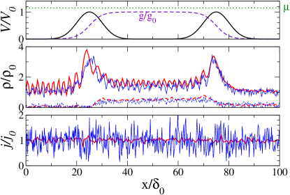
Figure 1: Density and current profiles of the scattering state in the near-resonant transport configuration for two different grid spacings $\delta=0.5\delta_{0}$ (thick red lines) and $\delta=0.2\delta_{0}$ (thin blue lines). The upper panel shows the external potential $V(x)$ (solid black line) as well as the interaction strength $g(x)$ (violet dashed line) according to Eqs. (39) and (40), respectively. The green dotted line marks the level of the chemical potential. The middle panel shows the total densities (upper solid lines) and the incoherent parts of the density according to Eq. (29) (lower dashed lines), while the lower panel shows the total currents, respectively for $\delta=0.5\delta_{0}$ (thick red lines) and $\delta=0.2\delta_{0}$ (thin blue lines). These tW calculations were done using $10^{6}$ random realizations of the vacuum fluctuations.

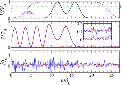
Figure 2: Same as Fig. 1 for the non-resonant transport configuration. Total and incoherent densities (middle panel) as well as total currents (lower panel) were computed for the grid spacings $\delta=0.2739\delta_{0}$ (thick red lines) and $\delta=0.1095\delta_{0}$ (thin blue lines), using again $10^{6}$ random realizations of the vacuum fluctuations.

Let us now verify these findings for the specific case of the transmission of a Bose-Einstein condensate through a symmetric double barrier potential. The latter is formed by a sequence of two Gaussian barriers, i.e.

$$V(x)=V_{0}\left(e^{-(x-x_{1})^{2}/(2\sigma^{2})}+e^{-(x-x_{2})^{2}/(2\sigma^{2})}\right)\,,$$ (39)

which are placed at the positions $x_{1}$ and $x_{2}$ and which have the same width $\sigma$. The spatial dependence of the one-dimensional interaction strength is chosen as

$$g(x)=g_{0}\left(\tanh\left[\frac{x-\tilde{x}_{1}}{\tilde{\sigma}}\right]-\tanh\left[\frac{x-\tilde{x}_{2}}{\tilde{\sigma}}\right]\right)\,.$$ (40)

For the sake of simplicity, we consider the coupling strength to the trap to be strongly localized in space, such that we can write $\sqrt{N}\kappa(x)=S_{0}\delta(x)$. This source emits a matter-wave beam whose chemical potential $\mu$ is tuned such that it is of the same order as the potential barrier height. In the absence of the scattering potential and the interaction, such a source would yield the homogeneous densities and currents

$$\rho_{0} = |S_{0}|^{2}m/(2\hbar^{2}\mu)\,,$$ (41)

$$j_{0} = \sqrt{2\mu/m}\rho_{0}\,.$$ (42)

We shall, in the following, consider two distinct transport scenarios: a near-resonant one with well-separated potential barriers, leading to nearly perfect transmission of the matter-wave beam, and a non-resonant one with overlapping barriers, leading to almost total reflection of the atoms. The former (near-resonant) configuration is obtained by choosing the parameters $x_{1}=\tilde{x}_{1}=25\delta_{0}$, $x_{2}=\tilde{x}_{2}=75\delta_{0}$, $\sigma=\tilde{\sigma}=5\delta_{0}$, $g_{0}=0.034V_{0}\delta_{0}$, $S_{0}=0.8V_{0}\sqrt{\delta_{0}}$, and $\mu=1.15V_{0}$. Here we introduce by $\delta_{0}=\hbar/\sqrt{mV_{0}}$ the characteristic length scale that corresponds to the barrier height $V_{0}$. For the latter (non-resonant) configuration, we choose $x_{1}=11.50\delta_{0}$, $x_{2}=15.88\delta_{0}$, $\sigma=1.095\delta_{0}$, $\tilde{x}_{1}=3.834\delta_{0}$, $\tilde{x}_{2}=24.1\delta_{0}$, $\tilde{\sigma}=1.643\delta_{0}$, $g_{0}=0.01826V_{0}\delta_{0}$, $S_{0}=1.974V_{0}\sqrt{\delta_{0}}$, and $\mu=0.727V_{0}$.

The practical numerical implementation of the tW method in this waveguide scattering problem is done in the same way as described in Ref. DujArgSch15PRA . In particular, we restrict the numerical representation of the waveguide to a finite spatial region ($0<x<100\delta_{0}$ in the near-resonant and $0<x<27.39\delta_{0}$ in the non-resonant case) in which the scattering potential and the interaction strength can be considered to be nonzero. Within the framework of the tW approach, the coupling to the two noninteracting “leads” on the left- and right-hand side gives then rise to a time-dependent quantum noise that enters into the scattering region DujArgSch15PRA . The decay of atoms to the leads, on the other hand, is modeled through smooth exterior complex scaling DujSaeSch14APB .

In the numerical practice, the source amplitude is slowly increased with time from zero to its maximal value $S_{0}$. Figure 1 shows the stationary density and current profiles that are numerically obtained after this ramping process in the near-resonant transport configuration, for two different choices for the numerical grid spacing $\delta$. We clearly see a nearly symmetric density profile, which is a signature of near-resonant transmission. The density maxima at the positions of the potential barriers as well as the slight enhancement of the density in the interacting region in between the barriers are explained by an effective decrease of the speed of the atoms due to energy conservation, which renders the atoms more likely to be detected there. As is indeed expected to occur in the presence of quasi-stationary scattering, the current profile, on the other hand, is fairly homogeneous within and outside the interacting region, apart from statistical fluctuations that arise from a finite Monte-Carlo sampling in the framework of the tW method.

Figure 2 shows the stationary density and current profiles in the non-resonant transport configuration, again for two different choices for the numerical grid spacing $\delta$. While the chosen chemical potential $\mu=0.727V_{0}$ lies rather close to a single-particle resonance of the double barrier potential, the presence of the atom-atom interaction gives rise to a significant shift of the effective resonance level to higher values of the chemical potential and thereby induces blocking of resonant transmission PauRicSch05PRL . Again, a fairly homogeneous current profile is obtained within and outside the interacting region.

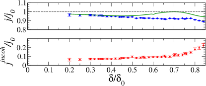
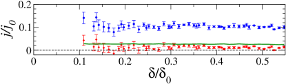
Figure 3: Total (blue circles) and incoherent transmissions (red diamonds) across the double barrier potential (39), obtained with the tW method for different values of the numerical grid spacing $\delta$ in the near-resonant (upper and middle panels) and the non-resonant transport configuration (lower panel) using the same parameters of the scattering system as for Figs. 1 and 2, respectively. The green solid lines show the results of a purely classical Gross-Pitaevskii calculation according to Ref. PauRicSch05PRL . The total and incoherent currents are calculated according to Eqs. (26) and (30), respectively, where we perform an additional average over the numerical grid points of the system (which then defines the depicted error bars). In both transport configurations, the total and the incoherent transmission tend to finite values in the limit of vanishing grid spacing $\delta\to 0$ rem_effort .

Figure 3 shows how the total and incoherent transmissions across the double barrier potential scale with the grid spacing $\delta$. We calculated for this purpose the average total current $j$ and the incoherent current $j^{\rm incoh}$ according to Eqs. (26) and (30), respectively, and performed an additional average over the numerical grid points of the system, in order to reduce the size of the statistical fluctuations. Clearly, we see that both the total and the incoherent transmission tend to finite values in the limit of vanishing grid spacing $\delta\to 0$, both for the near-resonant and the non-resonant transport configuration. This numerical observation confirms that the tW method is expected to yield consistent results in the continuous limit.

V Conclusion

In summary, we investigated the feasibility of the tW approach for the description of quasi-stationary scattering processes with interacting Bose-Einstein condensates in one-dimensional waveguides. While a discretization of position space is most conveniently introduced in order to apply the method in practice, we showed that consistent results are to be obtained in the continuous limit of vanishing grid spacing. This finding provides promising perspectives for the applicability of the tW method in the context of bosonic waveguide scattering processes. Indeed, judging from Ref. DujArgSch15PRA we expect that the tW method will yield reliable predictions in the presence of weak interaction strengths, similarly as for the Hartree-Fock-Bogoliubov method ErnPauSch10PRA or the Bogoliubov back-reaction method VarAng01PRL ; TikAngVar07PRA . It certainly breaks down in the presence of very strong interactions where genuinely quantum many-body approaches based on the density matrix renormalization group (DMRG) and the matrix-product state (MPS) method Whi92PRL ; Vid03PRL ; Vid04PRL ; VerPorCir04PRL ; DalO04JSM as well as on the Gutzwiller ansatz (see, e.g., Ref. Zak05PRA ) are more appropriate to describe the dynamics of the system.

We furthermore presented a semiclassical derivation of the tW approach in the framework of the van Vleck-Gutzwiller theory, which essentially relates this approach to the diagonal semiclassical approximation. This latter framework opens possibilities for a wider application of the tW method in the context of moderately interacting systems that exhibit chaotic classical dynamics. Indeed, while the conventional implementation of the tW method is not expected to yield reliable predictions for long evolution times that exceed the Ehrenfest time of such a chaotic system, average transport observables, which are obtained, e.g., in the presence of disorder, are nevertheless expected to be correctly reproduced by this approach provided we can safely assume classical ergodicity (and account for systematic quantum interference effects such as coherent backscattering in Fock space EngO14PRL ). This new semiclassical perspective of the tW approach will also form a useful basis for the development of a truly semiclassical van Vleck-Gutzwiller (or Herman-Kluk) approach that is able to capture interference effects beyond the diagonal approximation EngO14PRL ; SimStr14PRA ; EngUrbRic14xxx .

- (1) A. Micheli, A. J. Daley, D. Jaksch, and P. Zoller Phys. Rev. Lett. 93, 140408 (2004).
- (2) B. T. Seaman, M. Krämer, D. Z. Anderson, and M. J. Holland Phys. Rev. A 75, 023615 (2007).
- (3) R. A. Pepino, J. Cooper, D. Z. Anderson, and M. J. Holland Phys. Rev. Lett. 103, 140405 (2009).
- (4) J. P. Brantut, J. Meineke, D. Stadler, S. Krinner, and T. Esslinger Science 337, 1069 (2012).
- (5) J. P. Brantut, C. Grenier, J. Meineke, D. Stadler, S. Krinner, C. Kollath, T. Esslinger, and A. Georges Science 342, 713 (2013).
- (6) M. Bruderer and W. Belzig Phys. Rev. A 85, 013623 (2012).
- (7) L. H. Kristinsdóttir, O. Karlström, J. Bjerlin, J. C. Cremon, P. Schlagheck, A. Wacker, and S. M. Reimann Phys. Rev. Lett. 110, 085303 (2013).
- (8) D. B. Gutman, Y. Gefen, and A. D. Mirlin Phys. Rev. B 85, 125102 (2012).
- (9) A. Ivanov, G. Kordas, A. Komnik, and S. Wimberger Eur. Phys. J. B 86, 345 (2013).
- (10) W. Guerin, J. F. Riou, J. P. Gaebler, V. Josse, P. Bouyer, and A. Aspect Phys. Rev. Lett. 97, 200402 (2006).
- (11) A. Couvert, M. Jeppesen, T. Kawalec, G. Reinaudi, R. Mathevet, and D. Guéry-Odelin EPL 83, 50001 (2008).
- (12) G. L. Gattobigio, A. Couvert, B. Georgeot, and D. Guéry-Odelin Phys. Rev. Lett. 107, 254104 (2011).
- (13) P. Leboeuf and N. Pavloff Phys. Rev. A 64, 033602 (2001).
- (14) I. Carusotto Phys. Rev. A 63, 023610 (2001).
- (15) T. Paul, K. Richter, and P. Schlagheck Phys. Rev. Lett. 94, 020404 (2005).
- (16) T. Paul, P. Leboeuf, N. Pavloff, K. Richter, and P. Schlagheck Phys. Rev. A 72, 063621 (2005).
- (17) T. Paul, M. Hartung, K. Richter, and P. Schlagheck Phys. Rev. A 76, 063605 (2007).
- (18) E. H. Lieb, R. Seiringer, and J. Yngvason Phys. Rev. A 61, 043602 (2000).
- (19) T. Ernst, T. Paul, and P. Schlagheck Phys. Rev. A 81, 013631 (2010).
- (20) C. Gardiner and P. Zoller, Quantum Noise, 3rd edition (Springer, Berlin, 2004).
- (21) M. J. Steel, M. K. Olsen, L. I. Plimak, P. D. Drummond, S. M. Tan, M. J. Collett, D. F. Walls, and R. Graham Phys. Rev. A 58, 4824 (1998).
- (22) A. Sinatra, C. Lobo, and Y. Castin J. Phys. B: At. Mol. Opt. Phys. 35, 3599 (2002).
- (23) A. Polkovnikov Ann. Phys. 325, 1790 (2010).
- (24) J. Dujardin, A. Argüelles, and P. Schlagheck Phys. Rev. A 91, 033614 (2015).
- (25) B. Opanchuk and P. D. Drummond J. Math. Phys. 54, 042107 (2013).
- (26) M. C. Gutzwiller, Chaos in Classical and Quantum Mechanics (Springer, New York, 1990).
- (27) T. Engl, J. Dujardin, A. Argüelles, P. Schlagheck, K. Richter, and J. D. Urbina Phys. Rev. Lett. 112, 140403 (2014).
- (28) A. Polkovnikov Phys. Rev. A 68, 053604 (2003).
- (29) A. Kamenev, Field Theory of Non-Equilibrium Systems (Cambridge University Press, Cambridge, 2011).
- (30) M. Olshanii Phys. Rev. Lett. 81(5), 938 (1998).
- (31) L. Simon and W. T. Strunz Phys. Rev. A 89, 052112 (2014).
- (32) T. Engl, J. D. Urbina, and K. Richter arXiv:1409.5684 (2014).
- (33) For the exact quantum mechanical equivalent of Eq. (20), would have to be replaced by the Wigner transform of the associated time-dependent operator which is unavailable in practice.
- (34) J. Dujardin, A. Saenz, and P. Schlagheck Appl. Phys. B 117, 765 (2014).
- (35) Note that the numerical effort that is necessary to compute the tW averages of the total and incoherent currents with good statistical convergence increases dramatically with decreasing grid spacing. We therefore do not show transmission data for grid spacings in the near-resonant and in the non-resonant case.
- (36) A. Vardi and J. R. Anglin Phys. Rev. Lett. 86, 568 (2001).
- (37) I. Tikhonenkov, J. R. Anglin, , and A. Vardi Phys. Rev. A 75 75, 013613 (2007).
- (38) S. R. White Phys. Rev. Lett. 69, 2863 (1992).
- (39) G. Vidal Phys. Rev. Lett. 91(October), 147902 (2003).
- (40) G. Vidal Phys. Rev. Lett. 93, 040502 (2004).
- (41) F. Verstraete, D. Porras, and J. I. Cirac Phys. Rev. Lett. 93(November), 227205 (2004).
- (42) A. J. Daley, C. Kollath, U. Schollwöck, and G. Vidal J. Stat. Mech. p. P04005 (2004).
- (43) J. Zakrzewski Phys. Rev. A 71, 043601 (2005).