Radio Emission from Weak Spherical Shocks in the Outskirts of Galaxy Clusters

1 INTRODUCTION

Cosmological hydrodynamic simulations have shown that shock waves may form due to supersonic flow motions in the baryonic intracluster medium (ICM) during the formation of the large scale structure in the Universe (e.g., Ryu et al., 2003; Kang et al., 2007; Vazza et al., 2009; Skillman et al., 2011). The time evolution of the spatial distribution of such shocks in numerical simulations (e.g., Vazza et al., 2012) indicates that shock surfaces behave like spherical bubbles blowing out from the cluster center, when major episodes of mergers or infalls from adjacent filaments occur Ṡhock surfaces seem to last only for a fraction of a dynamical time scale of clusters, i.e., $\sim 0.1t_{\rm dyn}\sim 100$ Myr. This implies that some cosmological shock waves are associated with merger induced outflows, and that spherical shock bubbles are likely to expand into the cluster outskirts with a decreasing density profile.

Observational evidence for shock bubbles can be found at the so-called “radio relics” detected in the outskirts of galaxy cluster, which are interpreted as synchrotron emitting structures containing relativistic electrons accelerated at weak ICM shocks ($M_{s}\sim 2-4$) (e.g., van Weeren et al., 2010, 2011; Nuza et al., 2012; Feretti et al., 2012; Brunetti & Jones, 2014). Some radio relics, for instance, the “Sausage relic” in galaxy cluster CIZA J2242.8+5301 and the “Toothbrush” relic in galaxy cluster 1RXS J0603.3+4214, have thin arc-like shapes of $\sim 50$ kpc in width and $\sim 1-2$ Mpc in length (van Weeren et al., 2010, 2012). They could be represented by a ribbon-like structure on a spherical shell projected onto the sky plane (e.g., van Weeren et al., 2010; Kang et al., 2012).

As shown in Fig. 1, the viewing depth of a relic shock structure can be parameterized by the extension angle $2\psi$, while the physical width of the postshock shell of radiating electrons is mainly determined by the advection length, $\Delta l_{\rm adv}(\gamma_{e})\approx u_{2}\cdot\rm{min}[t_{\rm age},t_{\rm rad}(\gamma_{e})]$, where $u_{2}$ is the flow speed behind the shock and $t_{\rm rad}(\gamma_{e})$ is the radiative cooling time scale for electrons with Lorentz factor, $\gamma_{e}$. It remains largely unknown how such a ribbon-like structure can be formed by the spherical outflows in galaxy clusters. We note, however, a recent study by Shimwell et al. (2015) who suggested that the uniform arc-like shape of some radio relics may trace the underlying region of pre-existing seed electrons remaining from an old radio lobe.

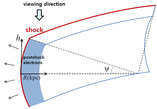
Figure 1: Schematic diagram showing a spherical shock surface (red) and the postshock electron distribution behind the shock adopted in this study. The shock surface is modeled as a Mpc-long ribbon on the spherical surface whose viewing depth can be defined by the extension angle $2\psi$. The depth of the postshock electron distribution behind the shock is determined by the advection length, $\Delta l_{\rm adv}\approx u_{2}\cdot t_{\rm age}$, for low energy electrons or the cooling length, $\Delta l_{\rm cool}(\gamma_{e})\approx u_{2}\cdot t_{rad}(\gamma_{e})$ for high energy electrons. The radio emissivity from CR electrons, $j_{\nu}(d)$ is calculated using the DSA simulation results in Paper I (where $d$ is the distance from the shock). The surface brightness is calculated by integrated $j_{\nu}(d)$ over the path along the line of sight (see Eq. [1]). If viewed from the top as indicated here, the projected image will have an arc-like shape similar to the Sausage relic in CIZA J2242.8+5301 (van Weeren et al., 2010).

According to diffusive shock acceleration (DSA) theory, cosmic-ray (CR) particles can be generated via Fermi 1st order process at collisionless shocks (Bell, 1978; Drury, 1983; Malkov & Drury, 2001). The test-particle DSA theory predicts that the CR energy spectrum at the shock position has a power-law energy spectrum, $N(E)\propto E^{-s}$, where $s=(\sigma+2)/(\sigma-1)$ and $\sigma=\rho_{2}/\rho_{1}$ is the shock compression ratio. Hereafter, we use the subscripts ‘1’ and ‘2’ to denote the conditions upstream and downstream of shock, respectively. Then the synchrotron radiation spectrum due to CR electrons at the shock location has a power-law form of $j_{\nu}(x_{s})\propto\nu^{-\alpha_{\rm inj}}$, where $\alpha_{\rm inj}=(s-1)/2$ is the injection index. Moreover, the volume-integrated synchrotron spectrum downstream of a planar shock becomes a simple power-law of $J_{\nu}\propto\nu^{-A_{\nu}}$ with $A_{\nu}=\alpha_{\rm inj}+0.5$ above a break frequency, since electrons cool via synchrotron and inverse-Compton (iC) losses behind the shock (e.g., Kang, 2011). Such spectral characteristics are commonly used to infer the shock properties (i.e., Mach number) of observed radio relic shocks (e.g., van Weeren et al., 2010; Stroe et al., 2014)

In Kang (2015) (Paper I), we calculated the electron acceleration at spherical shocks similar to Sedov-Taylor blast waves with $M_{s}\sim 2.5-4.5$, which expand into a hot uniform ICM. We found that the electron energy spectrum at the shock location has reached the steady state defined by the instantaneous shock parameters. So the spatially resolved, synchrotron radiation spectra at the shock could be described properly by the test-particle DSA predictions for planar shocks. However, the volume integrated spectra of both electrons and radiation evolve differently from those of planar shocks and exhibit some nonlinear signatures, depending on the time-dependent evolution of the shock parameters. For instance, the shock compression ratio $\sigma$ and the injection flux of CR electrons decrease in time, as the spherical shock expands and slows down, resulting in some curvatures in both electron and radiation spectra.

Magnetic fields play key roles in DSA at collisionless shocks and control the synchrotron cooling and emission of relativistic electrons. Observed magnetic field strength is found to decrease from $\sim 1-10~{}{\mu\rm G}$ in the core region to $\sim 0.1-1~{}{\mu\rm G}$ in the periphery of clusters (Feretti et al., 2012). On the other hand, it is well established that magnetic fields can be amplified via resonant and non-resonant instabilities induced by CR protons streaming upstream of strong shocks (Bell, 1978; Lucek & Bell, 2000; Bell, 2004). Recently, Caprioli & Spitkovsky (2014) has shown that the magnetic field amplification (MFA) factor scales with the Alfvénic Mach number, $M_{A}$, and the CR proton acceleration efficiency as $\langle\delta B/B\rangle^{2}\sim$ $3M_{A}(P_{\rm cr,2}/\rho_{1}u_{s}^{2})$. Here $\delta B$ is the turbulent magnetic fields perpendicular to the mean background magnetic fields, $\rho_{1}$ is the upstream gas density, and $P_{\rm cr,2}$ is the downstream CR pressure. For typical cluster shocks with $3\lesssim M_{s}\lesssim 5$ and $M_{A}\sim 10$ (Ryu et al., 2003), the MFA factor due to the streaming stabilities is expected be rather small but not negligible, $\langle\delta B/B\rangle^{2}\sim 0.3-1.5$. However, it has not yet been fully understood how magnetic fields may be amplified in both upstream and downstream of a weak shock in high beta ICM plasmas with $\beta_{p}=P_{g}/P_{B}\sim 100$.

Therefore, in Paper I, we considered several models with decaying postshock magnetic fields, in which the downstream magnetic field, $B_{d}(r)$, decreases behind the shock with a scale height of 100-150 kpc. We found that the impacts of different $B_{d}(r)$ profiles on the spatial distribution of the electron energy spectrum, $N_{e}(r,\gamma_{e})$, is not substantial, because iC scattering off cosmic background photons provides the baseline cooling rate. Any variations in $N_{e}(r,\gamma_{e})$ is smoothed out in the spatial distribution of the synchrotron emissivity, $j_{\nu}(r)$, because electrons in a broad range of $\gamma_{e}$ contribute to $j_{\nu}$ at a given frequency. We note, however, that the $B^{2}$ dependence of the synchrotron emissivity ($j_{\nu}\propto N_{e}B^{2}$) can become significant in some cases. Moreover, any nonlinear features due to the spatial variations of $N_{e}(r,\gamma_{e})$ and $B_{d}(r)$ are mostly averaged out, leaving only subtle signatures in the volume integrated spectrum, $J_{\nu}$.

For the case with a constant background density (e.g., MF1-3 model in Paper 1), the shock speed decreases approximately as $u_{s}\propto t^{-3/5}$. In fact, it has not been examined, through cosmological hydrodynamic simulations, whether these shock bubbles would accelerate or decelerate as they propagate into the cluster outskirts with a decreasing density profile. In this study, we have performed additional DSA simulations, in which the initial Sedov blast wave propagates into the background medium with $\rho_{u}\propto r^{-n}$, where $r$ is the radial distance from the cluster center and $n=2-4$. This effectively mimics a blast wave that expands into a constant-density core surrounded by an isothermal halo with a decreasing pressure profile. In these new runs, the spherical shock decelerates much slowly, compared to $u_{s}\propto t^{-3/5}$, and the nonlinear effects due to the deceleration of the shock speed are expected to be reduced from what we observed in the uniform density models considered in Paper I.

Here we also have calculated the projected surface brightness, $I_{\nu}$, which depend on the three dimensional structure of the shock surfaces and the viewing direction. Because of the curvature in the model shock structure, synchrotron emissions from downstream electrons with different ages contribute to the surface brightness along a given line-of-sight (i.e., projection effects). So the observed spatial profile of $I_{\nu}(R)$ is calculated by assuming the geometrical configuration described in Fig. 1. Note that this model with a ribbon-like shock surface gave rise to radio flux profiles, $S_{\nu}(R)$, that were consistent with those of the the Sausage relic in CIZA J2242.8+5301 and the double relics in ZwCl0008.8+5215 (e.g., van Weeren et al., 2010, 2011; Kang et al., 2012).

In paper I, we demonstrated that the spectral index of the volume-integrated spectral index increases gradually from $A_{\nu}=\alpha_{\rm inj}$ to $A_{\nu}=\alpha_{\rm inj}+0.5$ over a broad frequency range, $\sim(0.1-10)\nu_{\rm br}$, where the break frequency is $\nu_{\rm br}\sim 0.5$ GHz at the shock age of about 50 Myr for the postshock magnetic fields $\sim 7~{}{\mu\rm G}$ (see Eq. [5]). Here we have explored whether such a transition can explain the broken power-law spectra observed in the radio relic in A2256 (Trasatti et al., 2014).

In the next section we describe the numerical calculations. The DSA simulation results of blast wave models with different postshock magnetic field profiles and with different background density profiles will be discussed in Section 3. A brief summary will be given in Section 4.

2 Numerical Calculations

In order to calculate DSA of CR electrons at spherical shocks, we have solved the time-dependent diffusion-convection equation for the pitch-angle-averaged phase space distribution function for CR electrons, $f_{e}(r,p,t)$, in the one-dimensional spherically symmetric geometry (Skilling, 1975). The test-particle version of CRASH (Cosmic-Ray Amr SHock) code in a comoving spherical grid was used (Kang & Jones, 2006). The details of the simulation set-up can be found in Paper 1.

For the initial conditions, we adopt a Sedov-Taylor similarity solution propagating into a uniform ICM with the following parameters: the ICM density, $n_{H,1}=10^{-3}~{}{\rm cm^{-3}}$, the ICM temperature, $T_{1}=5\times 10^{7}$K, the initial shock radius, $r_{s,i}=0.78{\rm Mpc}$, and the initial shock speed, $u_{s,i}=4.5\times 10^{3}~{}{\rm km~{}s^{-1}}$ with the sonic Mach number, $M_{s,i}=4.3$ at the onset of the simulation. The shock parameters change in time as the spherical shock expands out, depending on the upstream conditions in the cluster outskirts. For iC cooling, a redshift $z=0.2$ is chosen as a reference epoch, so $B_{\rm rad}=3.24~{}{\mu\rm G}\cdot(1+z)^{2}=4.7~{}{\mu\rm G}$.

The synchrotron emissivity, $j_{\nu}(r)$, at each shell is calculated (in units of ${\rm erg~{}cm^{-3}~{}s^{-1}~{}Hz^{-1}~{}str^{-1}}$), using the electron distribution function, $f_{e}(r,p,t)$, and the magnetic field profile, $B(r,t)$, from the DSA simulations. Then the radio intensity or surface brightness, $I_{\nu}\ ({\rm erg~{}cm^{-2}~{}s^{-1}~{}Hz^{-1}~{}str^{-1}})$, is calculated by integrating $j_{\nu}$ along the path length, $h$, as shown in Fig. 1:

$$I_{\nu}(R)=2\int_{0}^{h_{\rm max}}j_{\nu}(d)d{\it h}.$$ (1)

Here $R$ is the distance behind the projected shock edge in the plane of the sky and $d=r_{s}-r$ is the distance of a shell behind the shock, where $(r_{s}-d)^{2}=(r_{s}-R)^{2}+h^{2}$. The extension angle $\psi=10^{\circ}$ is assumed in this study.

The volume integrated emissivity, $J_{\nu}=\int j_{\nu}(r)dV$, is calculated by integrating $j_{\nu}$ over the downstream volume defined in Fig. 1.

The spectral indexes of $j_{\nu}(d)$, $J_{\nu}$, and $I_{\nu}(R)$ are defined as follows:

$$\alpha_{\nu_{i}-\nu_{i+1}}(d)=-{{d\ln j_{\nu}(d)}\over{d\ln\nu}},$$ (2)

$$A_{\nu_{i}-\nu_{i+1}}=-{{d\ln J_{\nu}}\over{d\ln\nu}},$$ (3)

$$B_{\nu_{i}-\nu_{i+1}}(R)=-{{d\ln I_{\nu}(R)}\over{d\ln\nu}},$$ (4)

estimated between $\nu_{i}$ and $\nu_{i+1}$. We chose the following three frequencies at the source, $\nu_{1}=240$ MHz, $\nu_{2}=600$ MHz, $\nu_{3}=1.4$ GHz in Figs. 2 and 4. Then the redshifted frequency for objects at a redshift $z$ is $\nu_{\rm obs,i}=\nu_{i}/(1+z)$.

Table 1.  Model Parameters

Model	$\rho_{u}(r)$	$B_{d}(r)$
MF1a	$\rho_{u}=\rho_{0}$	$B_{d}=7\mu$G
MF2	$\rho_{u}=\rho_{0}$	$B_{d}\propto\rho(r)$
MF3	$\rho_{u}=\rho_{0}$	$B_{d}\propto\sqrt{P(r)}$
BD1a	$\rho_{u}=\rho_{0}$	$B_{d}=7\mu$G
BD2	$\rho_{u}\propto r^{-2}$	$B_{d}=7\mu$G
BD2b	$\rho_{u}\propto r^{-2}$	$B_{d}\propto\sqrt{P(r)}$
BD3	$\rho_{u}\propto r^{-4}$	$B_{d}=7\mu$G
BD3b	$\rho_{u}\propto r^{-4}$	$B_{d}\propto\sqrt{P(r)}$

^a In fact MF1 and BD1 models are identical.

3 DSA SIMULATION RESULTS

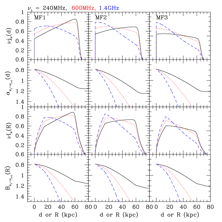
Figure 2: Spherical shock models with three different magnetic field profiles: MF1, MF2, and MF3. The results are shown at $t_{\rm age}=47$ Myr, when $r_{s}=0.96$Mpc, $u_{s}=3.4\times 10^{3}~{}{\rm km~{}s^{-1}}$ and $M_{s}=3.2$. In the upper two rows, spatial distributions of the synchrotron emissivity, $\nu_{i}j_{\nu_{i}}(r)$, and its spectral indexes, $\alpha_{\nu_{i}-\nu_{i+1}(r)}$ are plotted as a function of the postshock distance $d$ from the shock surface. In the lower two rows, the intensity $\nu_{i}I_{\nu_{i}}(R)$ and its spectral indexes, $B_{\nu_{i}-\nu_{i+1}}(R)$ are plotted as a function of the projected distance $R$ from the shock. The frequency is $\nu_{i}=$ 240 MHz (black solid line), 600 MHz (red dotted), 1.4 GHz (blue dashed), and 3 GHz for $i=1$, 2, 3, and 4. The downstream volume of radio-emitting electrons is assumed to have the same shape as the one illustrated in Fig. 1 with the extension angle $\psi=10^{\circ}$. Note that $j_{\nu}$ and $I_{\nu}$ are plotted in arbitrary units.

3.1 Shocks with Different Magnetic Field Profiles

As in the previous study of Kang et al. (2012), we adopt the postshock magnetic field strength $B_{2}\sim 7~{}{\mu\rm G}$ in order to explain the observed width of the Sausage relic ($\Delta l\sim 50$ kpc), while the preshock magnetic field strength is chosen to be $B_{1}\sim 2-3~{}{\mu\rm G}$. Since $B_{1}$ cannot be constrained directly from observations, it is adjusted so that $B_{2}$ becomes about 7 $~{}{\mu\rm G}$ after considering MFA or compression of the perpendicular components of magnetic fields across the shock.

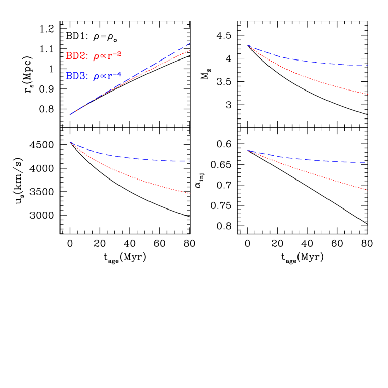
Figure 3: Evolution of spherical shock models with different background density profile, BD1 (black solid lines), BD2 (red dotted), and BD3 (blue dashed): shock radius, $R_{s}$, shock speed, $u_{s}$, sonic Mach number, $M_{s}$, and the DSA spectral index at the shock, $\alpha_{\rm inj}$.

We consider several models whose characteristics are summarized in Table 1. As described in Paper I, we adopt the following downstream magnetic field profile, $B_{d}(r)$ in MF models, in which the upstream density and temperature are uniform:

MF1: $B_{1}=2~{}{\mu\rm G}$ & $B_{2}=7~{}{\mu\rm G}$.

MF2: $B_{1}=3~{}{\mu\rm G}$, $B_{2}=B_{1}\sqrt{1/3+2\sigma^{2}/3}$,

& $B_{d}(r)=B_{2}\cdot(P(r)/P_{2})^{1/2}$ for $r<r_{s}$.

MF3: $B_{1}=3~{}{\mu\rm G}$, $B_{2}=B_{1}\sqrt{1/3+2\sigma^{2}/3}$,

& $B_{d}(r)=B_{2}\cdot(\rho(r)/\rho_{2})$ for $r<r_{s}$.

In Fig. 2 we compare these models at the shock age of 47 Myr. Note the evolution of the shock (i.e., $r_{s}(t)\propto t^{2/5}$ and $u_{s}(t)\propto t^{-3/5}$) is identical in the three models. Synchrotron emissivity scales with the electron energy spectrum and the magnetic field strength as $j_{\nu}\propto N_{e}(\gamma_{e})B^{2}$. Of course, the evolution of $N_{e}(\gamma_{e})$ in each MF model also depends on the assumed profile of $B_{d}(r)$ through DSA and synchrotron cooling. In MF1 model where $B_{d}(r)=B_{2}$, the spatial distribution of $j_{\nu}(d)$ at 240 MHz (black solid line) reveals dramatically the shock deceleration effects. It increases downstream behind the shock because of higher shock compression and higher electron injection flux at earlier time. On the other hand, $j_{\nu}(d)$ at 1.4 GHz (blue dashed line) decreases downstream behind the shock due to the fast synchrotron/iC cooling of high energy electrons.

The downstream increase of $j_{\nu}(d)$ at low frequencies is softened in the models with decaying postshock magnetic fields because of $B^{2}$ dependence of the synchrotron emissivity. In MF3 model, in which the downstream magnetic field decreases with the gas density behind the shocks, the spatial distributions of $j_{\nu}(d)$ at all three frequencies decrease downstream. Thus the downstream distribution of $j_{\nu}(d)$ depends on the shock speed evolution, $u_{s}(t)$ and the postshock $B_{d}(r)$ as well as the chosen frequency. In Paper I, we indicated, rather hastily, that signatures imprinted on synchrotron emission, $j_{\nu}(r)$, and its volume integrated spectrum, $J_{\nu}$, due to different postshock magnetic field profiles could be too subtle to detect. The main reason for this discrepancy is that we examined $\log j_{\nu}(r)$ in Paper I (see Fig. 6 there), while $\nu j_{\nu}(d)$ is plotted in Fig. 2.

As can be seen in the lower two rows of panels in Fig. 2, the surface brightness profiles, $I_{\nu}(R)$, are affected by the projection effects as well as the evolution of $u_{s}(t)$ and the spatial variation of $B_{d}(r)$. For instance, the gradual increase of $I_{\nu}$ just behind the shock up to $R_{\rm inf}<15$ kpc is due to the increase of the path length, and its inflection point, $R_{\rm inf}=r_{s}(1-\cos\psi)$, depends on the value of $\psi$. Beyond the inflection point, the path length decreases but $j_{\nu}(d)$ may increase or decrease depending on $u_{s}(t)$ and $B_{d}(r)$, resulting in a wide range of spatial profiles of $I_{\nu}(R)$.

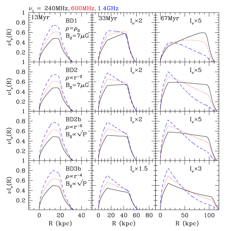
Figure 4: Spherical shock models with different background density and magnetic field profiles: BD1 (MF1), BD2, BD2b, and BD3b (from top to bottom panels). See Table 1 for the model parameters. Spatial distributions of the intensity $\nu I_{\nu}$ are shown at three shock ages, $t_{1}=13$ Myr, $t_{2}=33$ Myr, and $t_{3}=67$ Myr. The frequency is $\nu_{1}=240$ MHz (black solid line), $\nu_{2}=600$ MHz (red dotted), and $\nu_{1}=1.4$ GHz (blue dashed). The downstream volume of radio-emitting electrons is assumed to have the same shape as the one illustrated in Fig. 1 with the extension angle $\psi=10^{\circ}$. The intensity, $\nu I_{\nu}\cdot X$, is plotted in an arbitrary unit, where the numerical factor, $1\leq X\leq 5$, is adopted in order to plot the quantities in the linear scale.

Fig. 2 also demonstrate that the spectral indexes, $\alpha_{\nu_{i}-\nu_{i+1}}(d)$ and $B_{\nu_{i}-\nu_{i+1}}(R)$, at all three frequencies decrease behind the shock and do not show significant variations among the different MF models other than faster steepening of both indexes for a more rapid decay of $B_{d}(r)$.

In summary, at Sedov-Taylor type spherical shocks decelerating with $u_{s}\propto t^{-3/5}$, the distribution function, $N_{e}(r,\gamma_{e})$, of low energy electrons increases downstream behind the shock. As a result, the spatial distributions of the radio emissivity, $j_{\nu}(d)$, and the surface brightness, $I_{\nu}(R)$, at low radio frequencies ($<1$ GHz) could depend significantly on the postshock magnetic field profile. At high radio frequencies, such dependence becomes relatively weaker, because the postshock width of high energy electrons is much narrower and so the magnetic field profile far downstream has less influence on synchrotron emission. On the other hand, the spectral indexes, $\alpha_{\nu}$ and $B_{\nu}$, are relatively insensitive to those variations.

3.2 Shocks with Different Background Density Profile

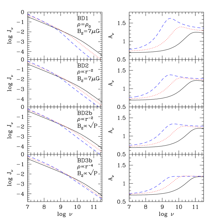
Figure 5: Same models shown as in Fig. 4. Volume integrated emissivity, $J_{\nu}$, and its spectral index, $A_{\nu}$, are shown at three different shock age, $t_{1}=13$ Myr (black solid lines), $t_{2}=33$ Myr (red dotted lines), and $t_{3}=67$ Myr (blue dashed lines).

In BD models, we assume that the initial blast wave propagates into an isothermal halo with a different density profile ($r>r_{s,i}$):

BD1: $\rho_{u}(r)=\rho_{0}$.

BD2: $\rho_{u}(r)=\rho_{0}\cdot({r/r_{s,i}})^{-2}$.

BD3: $\rho_{u}(r)=\rho_{0}\cdot({r/r_{s,i}})^{-4}$.

Again the upstream temperature ($T_{1}=5\times 10^{7}$ K) is uniform, and $B_{1}=2~{}{\mu\rm G}$ & $B_{2}=7~{}{\mu\rm G}$ for these models. In fact MF1 and BD1 models are identical. We also consider BD2b and BD3b models, in which the downstream magnetic field profile is the same as MF2, i.e., $B_{d}(r)\propto\sqrt{P(r)}$.

In the so-call beta model for the gas distribution for isothermal ICM, $\rho(r)\propto r^{-3\beta}$ in the outskirts of galaxy clusters (Sarazin, 1988). So BD2 model corresponds to the beta model with $\beta\approx 2/3$, which is consistent with typical X-ray brightness profile of observed X-ray clusters. Recall that in our simulations the spherical blast wave into a uniform ICM is adopted for the initial conditions. So we are effectively considering a spherical blast wave that propagates into a constant-density core (i.e., $\rho=\rho_{0}$ for $r<r_{s,i}$) surrounded by a isothermal halo with $\rho\propto r^{-n}$ (for $r>r_{s,i}$).

With the different background density (or gas pressure) profile, the shock speed evolves differently as it expands outward. Fig. 3 shows how the shock radius, $r_{s}(t)$, shock speed, $u_{s}(t)$, the sonic Mach number, $M_{s}(t)$, and the DSA spectral index at the shock position, $\alpha_{\rm inj}=3/[2(\sigma-1)]$, varies in time in BD models. As expected, the shock decelerates much slowly if the background pressure declines outward as in BD2 and BD3 models. In fact, the shock speed is almost constant in BD3 model. Hence these BD models allow us to explore the dependence of radio spectral properties for a wide range of the time evolution of the shock speed.

Fig. 4 compares the surface brightness profile, $I_{\nu}(R)$, at $\nu_{1}=240$ MHz (black solid lines), $\nu_{2}=600$ MHz (red dotted), and $\nu_{3}=1.4$ GHz (blue dashed) in the models with different $\rho_{u}$ and $B_{d}$. In BD1 model, the shock parameters are: $R_{s}=0.83$Mpc, $u_{s}=4.1\times 10^{3}~{}{\rm km~{}s^{-1}}$ and $M_{s}=3.9$ at $t_{1}=13$ Myr; $R_{s}=0.91$Mpc, $u_{s}=3.6\times 10^{3}~{}{\rm km~{}s^{-1}}$ and $M_{s}=3.4$ at $t_{2}=33$ Myr; $R_{s}=1.0$Mpc, $u_{s}=3.1\times 10^{3}~{}{\rm km~{}s^{-1}}$ and $M_{s}=2.9$ at $t_{3}=67$ Myr. Again, we can see that the surface brightness profile of $I_{\nu}(R)$ depends on the evolution of $u_{s}(t)$ and the spatial profile of $B_{d}(r)$.

The width of the radio structure, $\Delta l_{\rm adv}\sim t_{\rm age}u_{s}/\sigma$, increases with the shock age, while the amplitude of the surface brightness decreases in time (from left to right in Fig. 4). For high frequencies ($>1$ GHz), however, the width asymptotes to the cooling length, $\Delta l_{\rm cool}\sim t_{\rm rad}(\gamma_{e})u_{s}/\sigma$. So the postshock magnetic field strength can be obtained through $t_{\rm rad}(\gamma_{e})$ from high frequency observations. At low frequencies ($<1$ GHz) the surface brightness is affected by the evolution of $u_{s}(t)$ and the spatial variation of $B_{d}(r)$ as well as the projection effects, resulting in a wide range of spatial profiles of $I_{\nu}(R)$. This suggests that, if the radio surface brightness can be spatially resolved at several radio frequencies over $\sim(0.1-10)$ GHz, we may extract the time evolution of $u_{s}(t)$ as well as the shock age from low frequency observations. So it would be useful to compare multi-frequency radio observations with the intensity modeling that accounts for both shock evolution and projection effects.

The comparison of $I_{\nu}$ of MF1 (BD1) and MF2 models (see Fig. 2) demonstrates that the decaying postshock magnetic field could lessen the shock deceleration signatures in the surface brightness profile. If we compare $I_{\nu}$ of BD2 and BD2b models in Fig. 4, on the other hand, the difference in their profiles is much smaller than that between MF1 and MF2 models. This is because the the shock deceleration effects and the ensuing downstream increase of $N_{e}(r,\gamma_{e})$ are relatively milder in BD2 and BD2b models.

Next Fig. 5 compares the volume integrated spectrum, $J_{\nu}$, and its spectral index, $A_{\nu}$, at three different shock ages, $t_{\rm age}=$ 13 Myr (black solid), 33 Myr (red dotted), and 67 Myr (blue dashed) for the same set of models shown in Fig. 4.

For the test-particle power-law at planar shocks, the radio index $A_{\nu}$ is the same as $\alpha_{\rm inj}$ for $\nu<\nu_{\rm br}$, where

$$\nu_{\rm br}\approx 0.44{\rm GHz}\left({t_{\rm age}\over{50\rm Myr}}\right)^{-2}\left({B_{e,2}\over{8.4~{}{\mu\rm G}}}\right)^{-4}\left({B_{2}\over{7~{}{\mu\rm G}}}\right)$$ (5)

at the source. For $\nu>\nu_{\rm br}$, $A_{\nu}$ is expected to steepen to $\alpha_{\rm inj}+0.5$ due to synchrotron/iC cooling of electrons. Note that the smallest possible index is $\alpha_{\rm inj}=0.5$ at strong shocks, so $A_{\nu}=\alpha_{\rm inj}+0.5\geq 1.0$ above the break frequency. Also note that the observed (redshifted) break frequency corresponds to $\nu_{\rm br,obs}=\nu_{\rm br}/(1+z)$. If the shock age is $t_{\rm age}\sim 67$ Myr and $B_{2}\sim 7~{}{\mu\rm G}$, the observed break frequency becomes about 120 MHz for objects at $z=0.2$.

As can be seen in Fig. 5, however, the transition from $\alpha_{\rm inj}$ to $\alpha_{\rm inj}+0.5$ occurs gradually over about two orders of magnitude in frequency range. If the shock is 30-70 Myr old for the shock parameters considered here, the volume-integrated radio spectrum is expected to steepen gradually from 100 MHz to 10 GHz, instead of a sharp broken power-law with the break frequency at $\nu_{\rm br,obs}$. Such gradual steepening may explain why the volume-integrated radio spectrum of some relics was interpreted as a broken power-law with $A_{\nu}<1.0$ at low frequencies.

According to a recent observation of the relic in A2256, for example, the observed spectral index is $A_{351}^{1369}\approx 0.85$ between 351 and 1369 MHz and increases to $A_{1369}^{10450}\approx 1.0$ between 1369 and 10450 MHz (Trasatti et al., 2014). We estimated similar indexes for our $J_{\nu}$ between 355 and 1413 MHz, and between 1413 MHz and 10 GHz, using the DSA simulation results. In BD2b model, for example, at $t_{\rm age}=33$ Myr (red dotted line in Fig. 5), these spectral indexes are $A_{355}^{1413}\approx 0.85$ and $A_{1413}^{10000}\approx 1.07$. In BD3b model, again at $t_{\rm age}=33$ Myr, they are $A_{355}^{1413}\approx 0.83$ and $A_{1413}^{10000}\approx 1.03$. So if the shock age or the electron acceleration duration is about 30 Myr, relatively young compared to the dynamical time scale of typical clusters, the curved radio spectrum around 1 GHz can be explained by DSA at cluster shocks.

In the case of BD3b model, the spectral index behaves very similarly to that of a plane shock case (see Fig. 4 of Paper 1), since the shock speed is more or less constant in time. Departures from the predictions for the test-particle planar shock are the most severe in BD1 (MF1) model, while it becomes relatively milder in BD2 and BD3 models with decreasing halo density.

As shown in Paper I, any variations in the spatial distributions of $f_{e}(r)$ and $B_{d}(r)$ are smoothed in the volume integrated quantities such as $J_{\nu}$. So signatures imprinted on the volume-integrated emission due to different $B_{d}(r)$ (e.g., between BD2 and BD2b models) would be too subtle to detect.

4 SUMMARY

We have performed time-dependent DSA simulations for cosmic-ray (CR) electrons at decelerating spherical shocks with parameters relevant for weak cluster shocks: $u_{s}\approx(3.0-4.5)\times 10^{3}~{}{\rm km~{}s^{-1}}$ and $M_{s}\approx 3.0-4.3$. Several models with different postshock magnetic field profiles (MF1-3) and different upstream gas density profiles (BD1-3) were considered as summarized in Table 1. Using the synchrotron emissivity, $j_{\nu}(r)$, calculated from the CR electron energy spectra at these model shocks, the radio surface brightness profile, $I_{\nu}(R)$, and the volume integrated spectrum, $J_{\nu}$, were estimated by assuming a ribbon-like shock structure described in Fig. 1.

At low frequencies ($<1$ GHz) the surface brightness is affected by the evolution of $u_{s}(t)$ and the spatial variation of $B_{d}(r)$ as well as the projection effects , resulting in a wide range of spatial profiles of $I_{\nu}(R)$ (see Figs. 2 and 4). At high frequencies ($>1$ GHz), such dependences become relatively weaker, because the postshock width of high energy electrons is much narrower and so the magnetic field profile far downstream has less influence on synchrotron emission.

For low frequency observations, the width of radio relics increases with the shock age as $\Delta l_{\rm adv}\sim t_{\rm age}u_{s}/\sigma$, while it asymptotes to the cooling length, $\Delta l_{\rm cool}\sim t_{\rm rad}(\gamma_{e})u_{s}/\sigma$, for high frequencies. If the surface brightness can be spatially resolved at multi-frequency observations over $\sim(0.1-10)$ GHz, we may extract significant information about the time evolution of $u_{s}(t)$, the shock age, $t_{\rm age}$, and the postshock magnetic field strength, $B_{d}(r)$, through the detail modeling of DSA and projection effects. On the contrary, the spectral index of $I_{\nu}(R)$ behaves rather similarly in all the models considered here.

If the postshock magnetic field strength is about $7~{}{\mu\rm G}$, at the shock age of $\sim 30$ Myr, the volume-integrated radio spectrum has a break frequency, $\nu_{\rm br}\sim 1$ GHz, and steepens gradually with the spectral index from $\alpha_{\rm inj}$ to $\alpha_{\rm inj}+0.5$ over the frequency range of 0.1-10 GHz (see Fig. 5). Thus we suggest that such a curved spectrum could explain the observed spectrum of the relic in cluster A2256 (Trasatti et al., 2014).