Cascading Bandits: Learning to Rank in the Cascade Model

Abstract

A search engine usually outputs a list of $K$ web pages. The user examines this list, from the first web page to the last, and chooses the first attractive page. This model of user behavior is known as the cascade model. In this paper, we propose cascading bandits, a learning variant of the cascade model where the objective is to identify $K$ most attractive items. We formulate our problem as a stochastic combinatorial partial monitoring problem. We propose two algorithms for solving it, ${\tt CascadeUCB1}$ and ${\tt CascadeKL\mathchar 45\relax UCB}$. We also prove gap-dependent upper bounds on the regret of these algorithms and derive a lower bound on the regret in cascading bandits. The lower bound matches the upper bound of ${\tt CascadeKL\mathchar 45\relax UCB}$ up to a logarithmic factor. We experiment with our algorithms on several problems. The algorithms perform surprisingly well even when our modeling assumptions are violated.

1 Introduction

The cascade model is a popular model of user behavior in web search (Craswell et al., 2008). In this model, the user is recommended a list of $K$ items, such as web pages. The user examines the recommended list from the first item to the last, and selects the first attractive item. In web search, this is manifested as a click. The items before the first attractive item are not attractive, because the user examines these items but does not click on them. The items after the first attractive item are unobserved, because the user never examines these items. The optimal list, the list of $K$ items that maximizes the probability that the user finds an attractive item, are $K$ most attractive items. The cascade model is simple but effective in explaining the so-called position bias in historical click data (Craswell et al., 2008). Therefore, it is a reasonable model of user behavior.

In this paper, we propose an online learning variant of the cascade model, which we refer to as cascading bandits. In this model, the learning agent does not know the attraction probabilities of items. At time $t$, the agent recommends to the user a list of $K$ items out of $L$ items and then observes the index of the item that the user clicks. If the user clicks on an item, the agent receives a reward of one. The goal of the agent is to maximize its total reward, or equivalently to minimize its cumulative regret with respect to the list of $K$ most attractive items. Our learning problem can be viewed as a bandit problem where the reward of the agent is a part of its feedback. But the feedback is richer than the reward. Specifically, the agent knows that the items before the first attractive item are not attractive.

We make five contributions. First, we formulate a learning variant of the cascade model as a stochastic combinatorial partial monitoring problem. Second, we propose two algorithms for solving it, ${\tt CascadeUCB1}$ and ${\tt CascadeKL\mathchar 45\relax UCB}$. ${\tt CascadeUCB1}$ is motivated by ${\tt CombUCB1}$, a computationally and sample efficient algorithm for stochastic combinatorial semi-bandits (Gai et al., 2012; Kveton et al., 2015). ${\tt CascadeKL\mathchar 45\relax UCB}$ is motivated by ${\tt KL\mathchar 45\relax UCB}$ and we expect it to perform better when the attraction probabilities of items are low (Garivier & Cappe, 2011). This setting is common in the problems of our interest, such as web search. Third, we prove gap-dependent upper bounds on the regret of our algorithms. Fourth, we derive a lower bound on the regret in cascading bandits. This bound matches the upper bound of ${\tt CascadeKL\mathchar 45\relax UCB}$ up to a logarithmic factor. Finally, we experiment with our algorithms on several problems. They perform well even when our modeling assumptions are not satisfied.

Our paper is organized as follows. In Section 2, we review the cascade model. In Section 3, we introduce our learning problem and propose two UCB-like algorithms for solving it. In Section 4, we derive gap-dependent upper bounds on the regret of ${\tt CascadeUCB1}$ and ${\tt CascadeKL\mathchar 45\relax UCB}$. In addition, we prove a lower bound and discuss how it relates to our upper bounds. We experiment with our learning algorithms in Section 5. In Section 6, we review related work. We conclude in Section 7.

2 Background

Web pages in a search engine can be ranked automatically by fitting a model of user behavior in web search from historical click data (Radlinski & Joachims, 2005; Agichtein et al., 2006). The user is typically assumed to scan a list of $K$ web pages $A=(a_{1},\dots,a_{K})$, which we call items. The items belong to some ground set $E=\left\{1,\dots,L\right\}$, such as the set of all web pages. Many models of user behavior in web search exist (Becker et al., 2007; Craswell et al., 2008; Richardson et al., 2007). Each of them explains the clicks of the user differently. We focus on the cascade model.

The cascade model is a popular model of user behavior in web search (Craswell et al., 2008). In this model, the user scans a list of $K$ items $A=(a_{1},\dots,a_{K})\in\Pi_{K}(E)$ from the first item $a_{1}$ to the last $a_{K}$, where $\Pi_{K}(E)$ is the set of all $K$-permutations of set $E$. The model is parameterized by attraction probabilities $\bar{w}\in[0,1]^{E}$. After the user examines item $a_{k}$, the item attracts the user with probability $\bar{w}(a_{k})$, independently of the other items. If the user is attracted by item $a_{k}$, the user clicks on it and does not examine the remaining items. If the user is not attracted by item $a_{k}$, the user examines item $a_{k+1}$. It is easy to see that the probability that item $a_{k}$ is examined is $\prod_{i=1}^{k-1}(1-\bar{w}(a_{i}))$, and that the probability that at least one item in $A$ is attractive is $1-\prod_{i=1}^{K}(1-\bar{w}({a_{i}}))$. This objective is maximized by $K$ most attractive items.

The cascade model assumes that the user clicks on at most one item. In practice, the user may click on multiple items. The cascade model cannot explain this pattern. Therefore, the model was extended in several directions, for instance to take into account multiple clicks and the persistence of users (Chapelle & Zhang, 2009; Guo et al., 2009a, b). The extended models explain click data better than the cascade model. Nevertheless, the cascade model is still very attractive, because it is simpler and can be reasonably fit to click data. Therefore, as a first step towards understanding more complex models, we study an online variant of the cascade model in this work.

3 Cascading Bandits

We propose a learning variant of the cascade model (Section 3.1) and two computationally-efficient algorithms for solving it (Section 3.2). To simplify exposition, all random variables are written in bold.

3.1 Setting

We refer to our learning problem as a generalized cascading bandit. Formally, we represent the problem by a tuple $B=(E,P,K)$, where $E=\left\{1,\dots,L\right\}$ is a ground set of $L$ items, $P$ is a probability distribution over a unit hypercube $\left\{0,1\right\}^{E}$, and $K\leq L$ is the number of recommended items. We call the bandit generalized because the form of the distribution $P$ has not been specified yet.

Let $(\mathbf{w}_{t})_{t=1}^{n}$ be an i.i.d. sequence of $n$ weights drawn from $P$, where $\mathbf{w}_{t}\in\left\{0,1\right\}^{E}$ and $\mathbf{w}_{t}(e)$ is the preference of the user for item $e$ at time $t$. That is, $\mathbf{w}_{t}(e)=1$ if and only if item $e$ attracts the user at time $t$. The learning agent interacts with our problem as follows. At time $t$, the agent recommends a list of $K$ items $\mathbf{A}_{t}=(\mathbf{a}^{t}_{1},\dots,\mathbf{a}^{t}_{K})\in\Pi_{K}(E)$. The list is computed from the observations of the agent up to time $t$. The user examines the list, from the first item $\mathbf{a}^{t}_{1}$ to the last $\mathbf{a}^{t}_{K}$, and clicks on the first attractive item. If the user is not attracted by any item, the user does not click on any item. Then time increases to $t+1$.

The reward of the agent at time $t$ can be written in several forms. For instance, as $\max_{k}\mathbf{w}_{t}(\mathbf{a}^{t}_{k})$, at least one item in list $\mathbf{A}_{t}$ is attractive; or as $f(\mathbf{A}_{t},\mathbf{w}_{t})$, where:

$$f(A,w)=1-\prod_{k=1}^{K}(1-w(a_{k}))\,,$$

$A=(a_{1},\dots,a_{K})\in\Pi_{K}(E)$, and $w\in\left\{0,1\right\}^{E}$. This later algebraic form is particularly useful in our proofs.

The agent at time $t$ receives feedback:

$$\mathbf{C}_{t}=\operatorname*{arg\,min\,}\left\{1\leq k\leq K:\mathbf{w}_{t}(\mathbf{a}^{t}_{k})=1\right\}\,,$$

where we assume that $\operatorname*{arg\,min\,}\emptyset=\infty$. The feedback $\mathbf{C}_{t}$ is the click of the user. If $\mathbf{C}_{t}\leq K$, the user clicks on item $\mathbf{C}_{t}$. If $\mathbf{C}_{t}=\infty$, the user does not click on any item. Since the user clicks on the first attractive item in the list, we can determine the observed weights of all recommended items at time $t$ from $\mathbf{C}_{t}$. In particular, note that:

$$\mathbf{w}_{t}(\mathbf{a}^{t}_{k})=\mathds{1}\!\left\{\mathbf{C}_{t}=k\right\}\quad k=1,\dots,\min\left\{\mathbf{C}_{t},K\right\}\,.$$ (1)

We say that item $e$ is observed at time $t$ if $e=\mathbf{a}^{t}_{k}$ for some $1\leq k\leq\min\left\{\mathbf{C}_{t},K\right\}$.

In the cascade model (Section 2), the weights of the items in the ground set $E$ are distributed independently. We also make this assumption.

Assumption 1.

The weights $w$ are distributed as:

$$P(w)=\prod_{e\in E}P_{e}(w(e))\,,$$

where $P_{e}$ is a Bernoulli distribution with mean $\bar{w}(e)$.

Under this assumption, we refer to our learning problem as a cascading bandit. In this new problem, the weight of any item at time $t$ is drawn independently of the weights of the other items at that, or any other, time. This assumption has profound consequences and leads to a particularly efficient learning algorithm in Section 3.2. More specifically, under our assumption, the expected reward for list $A\in\Pi_{K}(E)$, the probability that at least one item in $A$ is attractive, can be expressed as $\mathbb{E}\left[f(A,\mathbf{w})\right]=f(A,\bar{w})$, and depends only on the attraction probabilities of individual items in $A$.

The agent’s policy is evaluated by its expected cumulative regret:

$$R(n)=\mathbb{E}\left[\sum_{t=1}^{n}R(\mathbf{A}_{t},\mathbf{w}_{t})\right]\,,$$

where $R(\mathbf{A}_{t},\mathbf{w}_{t})=f(A^{\ast},\mathbf{w}_{t})-f(\mathbf{A}_{t},\mathbf{w}_{t})$ is the instantaneous stochastic regret of the agent at time $t$ and:

$$A^{\ast}=\operatorname*{arg\,max\,}_{A\in\Pi_{K}(E)}f(A,\bar{w})$$

is the optimal list of items, the list that maximized the reward at any time $t$. Since $f$ is invariant to the permutation of $A$, there exist at least $K!$ optimal lists. For simplicity of exposition, we assume that the optimal solution, as a set, is unique.

3.2 Algorithms

We propose two algorithms for solving cascading bandits, ${\tt CascadeUCB1}$ and ${\tt CascadeKL\mathchar 45\relax UCB}$. ${\tt CascadeUCB1}$ is motivated by ${\tt UCB1}$ (Auer et al., 2002) and ${\tt CascadeKL\mathchar 45\relax UCB}$ is motivated by ${\tt KL\mathchar 45\relax UCB}$ (Garivier & Cappe, 2011).

The pseudocode of both algorithms is in Algorithm 1. The algorithms are similar and differ only in how they estimate the upper confidence bound (UCB) $\mathbf{U}_{t}(e)$ on the attraction probability of item $e$ at time $t$. After that, they recommend a list of $K$ items with largest UCBs:

$$\mathbf{A}_{t}=\operatorname*{arg\,max\,}_{A\in\Pi_{K}(E)}f(A,\mathbf{U}_{t})\,.$$ (2)

Note that $\mathbf{A}_{t}$ is determined only up to a permutation of the items in it. The payoff is not affected by this ordering. But the observations are. For now, we leave the order of items unspecified and return to it later in our discussions. After the user provides feedback $\mathbf{C}_{t}$, the algorithms update their estimates of the attraction probabilities $\bar{w}(e)$ based on (1), for all $e=\mathbf{a}^{t}_{k}$ where $k\leq\mathbf{C}_{t}$.

Algorithm 1 UCB-like algorithm for cascading bandits.

  // Initialization

  Observe $\mathbf{w}_{0}\sim P$

  $\forall e\in E:\mathbf{T}_{0}(e)\leftarrow 1$

  $\forall e\in E:\hat{\mathbf{w}}_{1}(e)\leftarrow\mathbf{w}_{0}(e)$

  

  for all $t=1,\dots,n$ do

     Compute UCBs $\mathbf{U}_{t}(e)$ (Section 3.2)

     

     // Recommend a list of $K$ items and get feedback

     Let $\mathbf{a}^{t}_{1},\dots,\mathbf{a}^{t}_{K}$ be $K$ items with largest UCBs

     $\mathbf{A}_{t}\leftarrow(\mathbf{a}^{t}_{1},\dots,\mathbf{a}^{t}_{K})$

     Observe click $\mathbf{C}_{t}\in\left\{1,\dots,K,\infty\right\}$

     

     // Update statistics

     $\forall e\in E:\mathbf{T}_{t}(e)\leftarrow\mathbf{T}_{t-1}(e)$

     for all $k=1,\dots,\min\left\{\mathbf{C}_{t},K\right\}$ do

        $e\leftarrow\mathbf{a}^{t}_{k}$

        $\mathbf{T}_{t}(e)\leftarrow\mathbf{T}_{t}(e)+1$

        $\displaystyle\hat{\mathbf{w}}_{\mathbf{T}_{t}(e)}(e)\leftarrow\frac{\mathbf{T}_{t-1}(e)\hat{\mathbf{w}}_{\mathbf{T}_{t-1}(e)}(e)+\mathds{1}\!\left\{\mathbf{C}_{t}=k\right\}}{\mathbf{T}_{t}(e)}$

The UCBs are computed as follows. In ${\tt CascadeUCB1}$, the UCB on the attraction probability of item $e$ at time $t$ is:

$$\mathbf{U}_{t}(e)=\hat{\mathbf{w}}_{\mathbf{T}_{t-1}(e)}(e)+c_{t-1,\mathbf{T}_{t-1}(e)}\,,$$

where $\hat{\mathbf{w}}_{s}(e)$ is the average of $s$ observed weights of item $e$, $\mathbf{T}_{t}(e)$ is the number of times that item $e$ is observed in $t$ steps, and:

$$c_{t,s}=\sqrt{(1.5\log t)/s}$$

is the radius of a confidence interval around $\hat{\mathbf{w}}_{s}(e)$ after $t$ steps such that $\bar{w}(e)\in[\hat{\mathbf{w}}_{s}(e)-c_{t,s},\hat{\mathbf{w}}_{s}(e)+c_{t,s}]$ holds with high probability. In ${\tt CascadeKL\mathchar 45\relax UCB}$, the UCB on the attraction probability of item $e$ at time $t$ is:

$$\mathbf{U}_{t}(e)=\max\{q\in[\hat{\mathbf{w}}_{\mathbf{T}_{t-1}(e)}(e),1]:$$

$$\quad\mathbf{T}_{t-1}(e)D_{\mathrm{KL}}(\hat{\mathbf{w}}_{\mathbf{T}_{t-1}(e)}(e)\,\|\,q)\leq\log t+3\log\log t\}\,,$$

where $D_{\mathrm{KL}}(p\,\|\,q)$ is the Kullback-Leibler (KL) divergence between two Bernoulli random variables with means $p$ and $q$. Since $D_{\mathrm{KL}}(p\,\|\,q)$ is an increasing function of $q$ for $q\geq p$, the above UCB can be computed efficiently.

3.3 Initialization

Both algorithms are initialized by one sample $\mathbf{w}_{0}$ from $P$. Such a sample can be generated in $O(L)$ steps, by recommending each item once as the first item in the list.

4 Analysis

Our analysis exploits the fact that our reward and feedback models are closely connected. More specifically, we show in Section 4.1 that the learning algorithm can suffer regret only if it recommends suboptimal items that are observed. Based on this result, we prove upper bounds on the $n$-step regret of ${\tt CascadeUCB1}$ and ${\tt CascadeKL\mathchar 45\relax UCB}$ (Section 4.2). We prove a lower bound on the regret in cascading bandits in Section 4.3. We discuss our results in Section 4.4.

4.1 Regret Decomposition

Without loss of generality, we assume that the items in the ground set $E$ are sorted in decreasing order of their attraction probabilities, $\bar{w}(1)\geq\ldots\geq\bar{w}(L)$. In this setting, the optimal solution is $A^{\ast}=(1,\dots,K)$, and contains the first $K$ items in $E$. We say that item $e$ is optimal if $1\leq e\leq K$. Similarly, we say that item $e$ is suboptimal if $K<e\leq L$. The gap between the attraction probabilities of suboptimal item $e$ and optimal item $e^{\ast}$:

$$\Delta_{e,e^{\ast}}=\bar{w}(e^{\ast})-\bar{w}(e)$$ (3)

measures the hardness of discriminating the items. Whenever convenient, we view an ordered list of items as the set of items on that list.

Our main technical lemma is below. The lemma says that the expected value of the difference of the products of random variables can be written in a particularly useful form.

Lemma 1.

Let $A=(a_{1},\dots,a_{K})$ and $B=(b_{1},\dots,b_{K})$ be any two lists of $K$ items from $\Pi_{K}(E)$ such that $a_{i}=b_{j}$ only if $i=j$. Let $\mathbf{w}\sim P$ in 1. Then:

$$\mathbb{E}\left[\prod_{k=1}^{K}\mathbf{w}(a_{k})-\prod_{k=1}^{K}\mathbf{w}(b_{k})\right]=\sum_{k=1}^{K}\mathbb{E}\left[\prod_{i=1}^{k-1}\mathbf{w}(a_{i})\right]\times{}$$

$$\quad\mathbb{E}\left[\mathbf{w}(a_{k})-\mathbf{w}(b_{k})\right]\left(\prod_{j=k+1}^{K}\mathbb{E}\left[\mathbf{w}(b_{j})\right]\right)\,.$$

Proof.

The claim is proved in Appendix B.  

Let:

$$\mathcal{H}_{t}=(\mathbf{A}_{1},\mathbf{C}_{1},\dots,\mathbf{A}_{t-1},\mathbf{C}_{t-1},\mathbf{A}_{t})$$ (4)

be the history of the learning agent up to choosing $\mathbf{A}_{t}$, the first $t-1$ observations and $t$ actions. Let $\mathbb{E}_{t}\left[\cdot\right]=\mathbb{E}\left[\cdot\,\middle|\,\mathcal{H}_{t}\right]$ be the conditional expectation given history $\mathcal{H}_{t}$. We bound $\mathbb{E}_{t}\left[R(\mathbf{A}_{t},\mathbf{w}_{t})\right]$, the expected regret conditioned on history $\mathcal{H}_{t}$, as follows.

Theorem 1.

For any item $e$ and optimal item $e^{\ast}$, let:

$$G_{e,e^{\ast},t} =\{\exists 1\leq k\leq K\text{ s.t. }\mathbf{a}^{t}_{k}=e,\ \pi_{t}(k)=e^{\ast},$$ (5)

$$\phantom{{}=\{}\mathbf{w}_{t}(\mathbf{a}^{t}_{1})=\ldots=\mathbf{w}_{t}(\mathbf{a}^{t}_{k-1})=0\}$$

be the event that item $e$ is chosen instead of item $e^{\ast}$ at time $t$, and that item $e$ is observed. Then there exists a permutation $\pi_{t}$ of optimal items $\left\{1,\dots,K\right\}$, which is a deterministic function of $\mathcal{H}_{t}$, such that $\mathbf{U}_{t}(\mathbf{a}^{t}_{k})\geq\mathbf{U}_{t}(\pi_{t}(k))$ for all $k$. Moreover:

$$\mathbb{E}_{t}\left[R(\mathbf{A}_{t},\mathbf{w}_{t})\right] \leq\sum_{e=K+1}^{L}\sum_{e^{\ast}=1}^{K}\Delta_{e,e^{\ast}}\mathbb{E}_{t}\left[\mathds{1}\!\left\{G_{e,e^{\ast},t}\right\}\right]$$

$$\mathbb{E}_{t}\left[R(\mathbf{A}_{t},\mathbf{w}_{t})\right] \geq\alpha\sum_{e=K+1}^{L}\sum_{e^{\ast}=1}^{K}\Delta_{e,e^{\ast}}\,\mathbb{E}_{t}\left[\mathds{1}\!\left\{G_{e,e^{\ast},t}\right\}\right]\,,$$

where $\alpha=(1-\bar{w}(1))^{K-1}$ and $\bar{w}(1)$ is the attraction probability of the most attractive item.

Proof.

We define $\pi_{t}$ as follows. For any $k$, if the $k$-th item in $\mathbf{A}_{t}$ is optimal, we place this item at position $k$, $\pi_{t}(k)=\mathbf{a}^{t}_{k}$. The remaining optimal items are positioned arbitrarily. Since $A^{\ast}$ is optimal with respect to $\bar{w}$, $\bar{w}(\mathbf{a}^{t}_{k})\leq\bar{w}(\pi_{t}(k))$ for all $k$. Similarly, since $\mathbf{A}_{t}$ is optimal with respect to $\mathbf{U}_{t}$, $\mathbf{U}_{t}(\mathbf{a}^{t}_{k})\geq\mathbf{U}_{t}(\pi_{t}(k))$ for all $k$. Therefore, $\pi_{t}$ is the desired permutation.

The permutation $\pi_{t}$ reorders the optimal items in a convenient way. Since time $t$ is fixed, let $\mathbf{a}^{\ast}_{k}=\pi_{t}(k)$. Then:

$$\mathbb{E}_{t}\left[R(\mathbf{A}_{t},\mathbf{w}_{t})\right]=$$

$$\quad\mathbb{E}_{t}\left[\prod_{k=1}^{K}(1-\mathbf{w}_{t}(\mathbf{a}^{t}_{k}))-\prod_{k=1}^{K}(1-\mathbf{w}_{t}(\mathbf{a}^{\ast}_{k}))\right]\,.$$

Now we exploit the fact that the entries of $\mathbf{w}_{t}$ are independent of each other given $\mathcal{H}_{t}$. By Lemma 1, we can rewrite the right-hand side of the above equation as:

$$\sum_{k=1}^{K}\mathbb{E}_{t}\left[\prod_{i=1}^{k-1}(1-\mathbf{w}_{t}(\mathbf{a}^{t}_{i}))\right]\mathbb{E}_{t}\left[\mathbf{w}_{t}(\mathbf{a}^{\ast}_{k})-\mathbf{w}_{t}(\mathbf{a}^{t}_{k})\right]\times{}$$

$$\quad\left(\prod_{j=k+1}^{K}\mathbb{E}_{t}\left[1-\mathbf{w}_{t}(\mathbf{a}^{\ast}_{j})\right]\right)\,.$$

Note that $\mathbb{E}_{t}\left[\mathbf{w}_{t}(\mathbf{a}^{\ast}_{k})-\mathbf{w}_{t}(\mathbf{a}^{t}_{k})\right]=\Delta_{\mathbf{a}^{t}_{k},\mathbf{a}^{\ast}_{k}}$. Furthermore, $\prod_{i=1}^{k-1}(1-\mathbf{w}_{t}(\mathbf{a}^{t}_{i}))=\mathds{1}\!\left\{G_{\mathbf{a}^{t}_{k},\mathbf{a}^{\ast}_{k},t}\right\}$ by conditioning on $\mathcal{H}_{t}$. Therefore, we get that $\mathbb{E}_{t}\left[R(\mathbf{A}_{t},\mathbf{w}_{t})\right]$ is equal to:

$$\sum_{k=1}^{K}\Delta_{\mathbf{a}^{t}_{k},\mathbf{a}^{\ast}_{k}}\mathbb{E}_{t}\left[\mathds{1}\!\left\{G_{\mathbf{a}^{t}_{k},\mathbf{a}^{\ast}_{k},t}\right\}\right]\prod_{j=k+1}^{K}\mathbb{E}_{t}\left[1-\mathbf{w}_{t}(\mathbf{a}^{\ast}_{j})\right]\,.$$

By definition of $\pi_{t}$, $\Delta_{\mathbf{a}^{t}_{k},\mathbf{a}^{\ast}_{k}}=0$ when item $\mathbf{a}^{t}_{k}$ is optimal. In addition, $1-\bar{w}(1)\leq\mathbb{E}_{t}\left[1-\mathbf{w}_{t}(\mathbf{a}^{\ast}_{j})\right]\leq 1$ for any optimal $\mathbf{a}^{\ast}_{j}$. Our upper and lower bounds on $\mathbb{E}_{t}\left[R(\mathbf{A}_{t},\mathbf{w}_{t})\right]$ follow from these observations.  

4.2 Upper Bounds

In this section, we derive two upper bounds on the $n$-step regret of ${\tt CascadeUCB1}$ and ${\tt CascadeKL\mathchar 45\relax UCB}$.

Theorem 2.

The expected $n$-step regret of ${\tt CascadeUCB1}$ is bounded as:

$$R(n)\leq\sum_{e=K+1}^{L}\frac{12}{\Delta_{e,K}}\log n+\frac{\pi^{2}}{3}L\,.$$

Proof.

The complete proof is in Section A.1. The proof has four main steps. First, we bound the regret of the event that $\bar{w}(e)$ is outside of the high-probability confidence interval around $\hat{\mathbf{w}}_{\mathbf{T}_{t-1}(e)}(e)$ for at least one item $e$. Second, we decompose the regret at time $t$ and apply Theorem 1 to bound it from above. Third, we bound the number of times that each suboptimal item is chosen in $n$ steps. Fourth, we peel off an extra factor of $K$ in our upper bound based on Kveton et al. (2014a). Finally, we sum up the regret of all suboptimal items.  

Theorem 3.

For any $\varepsilon>0$, the expected $n$-step regret of ${\tt CascadeKL\mathchar 45\relax UCB}$ is bounded as:

$$R(n) \leq\sum_{e=K+1}^{L}\frac{(1+\varepsilon)\Delta_{e,K}(1+\log(1/\Delta_{e,K}))}{D_{\mathrm{KL}}(\bar{w}(e)\,\|\,\bar{w}(K))}\times{}$$

$$\qquad\qquad\ (\log n+3\log\log n)+C\,,$$

where $C=KL\frac{C_{2}(\varepsilon)}{n^{\beta(\varepsilon)}}+7K\log\log n$, and the constants $C_{2}(\varepsilon)$ and $\beta(\varepsilon)$ are defined in Garivier & Cappe (2011).

Proof.

The complete proof is in Section A.2. The proof has four main steps. First, we bound the regret of the event that $\bar{w}(e)>\mathbf{U}_{t}(e)$ for at least one optimal item $e$. Second, we decompose the regret at time $t$ and apply Theorem 1 to bound it from above. Third, we bound the number of times that each suboptimal item is chosen in $n$ steps. Fourth, we derive a new peeling argument for ${\tt KL\mathchar 45\relax UCB}$ (Lemma 2) and eliminate an extra factor of $K$ in our upper bound. Finally, we sum up the regret of all suboptimal items.  

4.3 Lower Bound

Our lower bound is derived on the following problem. The ground set contains $L$ items $E=\left\{1,\dots,L\right\}$. The distribution $P$ is a product of $L$ Bernoulli distributions $P_{e}$, each of which is parameterized by:

$$\bar{w}(e)=\begin{cases}p&e\leq K\\ p-\Delta&\text{otherwise}\,,\end{cases}$$ (6)

where $\Delta\in(0,p)$ is the gap between any optimal and suboptimal items. We refer to the resulting bandit problem as $B_{\mathrm{LB}}(L,K,p,\Delta)$; and parameterize it by $L$, $K$, $p$, and $\Delta$.

Our lower bound holds for consistent algorithms. We say that the algorithm is consistent if for any cascading bandit, any suboptimal list $A$, and any $\alpha>0$, $\mathbb{E}\left[\mathbf{T}_{n}(A)\right]=o(n^{\alpha})$, where $\mathbf{T}_{n}(A)$ is the number of times that list $A$ is recommended in $n$ steps. Note that the restriction to the consistent algorithms is without loss of generality. The reason is that any inconsistent algorithm must suffer polynomial regret on some instance of cascading bandits, and therefore cannot achieve logarithmic regret on every instance of our problem, similarly to ${\tt CascadeUCB1}$ and ${\tt CascadeKL\mathchar 45\relax UCB}$.

Theorem 4.

For any cascading bandit $B_{\mathrm{LB}}$, the regret of any consistent algorithm is bounded from below as:

$$\liminf_{n\to\infty}\frac{R(n)}{\log n}\geq\frac{(L-K)\Delta(1-p)^{K-1}}{D_{\mathrm{KL}}(p-\Delta\,\|\,p)}\,.$$

Proof.

By Theorem 1, the expected regret at time $t$ conditioned on history $\mathcal{H}_{t}$ is bounded from below as:

$$\mathbb{E}_{t}\left[R(\mathbf{A}_{t},\mathbf{w}_{t})\right]\geq\Delta(1-p)^{K-1}\!\!\!\!\sum_{e=K+1}^{L}\sum_{e^{\ast}=1}^{K}\!\mathbb{E}\left[\mathds{1}\!\left\{G_{e,e^{\ast},t}\right\}\right]\,.$$

Based on this result, the $n$-step regret is bounded as:

$$R(n) \geq\Delta(1-p)^{K-1}\sum_{e=K+1}^{L}\mathbb{E}\left[\sum_{t=1}^{n}\sum_{e^{\ast}=1}^{K}\mathds{1}\!\left\{G_{e,e^{\ast},t}\right\}\right]$$

$$=\Delta(1-p)^{K-1}\sum_{e=K+1}^{L}\mathbb{E}\left[\mathbf{T}_{n}(e)\right]\,,$$

where the last step is based on the fact that the observation counter of item $e$ increases if and only if event $G_{e,e^{\ast},t}$ happens. By the work of Lai & Robbins (1985), we have that for any suboptimal item $e$:

$$\liminf_{n\to\infty}\frac{\mathbb{E}\left[\mathbf{T}_{n}(e)\right]}{\log n}\geq\frac{1}{D_{\mathrm{KL}}(p-\Delta\,\|\,p)}\,.$$

Otherwise, the learning algorithm is unable to distinguish instances of our problem where item $e$ is optimal, and thus is not consistent. Finally, we chain all inequalities and get:

$$\liminf_{n\to\infty}\frac{R(n)}{\log n}\geq\frac{(L-K)\Delta(1-p)^{K-1}}{D_{\mathrm{KL}}(p-\Delta\,\|\,p)}\,.$$

This concludes our proof.  

Our lower bound is practical when no optimal item is very attractive, $p<1/K$. In this case, the learning agent must learn $K$ sufficiently attractive items to identify the optimal solution. This lower bound is not practical when $p$ is close to $1$, because it becomes exponentially small. In this case, other lower bounds would be more practical. For instance, consider a problem with $L$ items where item $1$ is attractive with probability one and all other items are attractive with probability zero. The optimal list of $K$ items in this problem can be found in $L/(2K)$ steps in expectation.

4.4 Discussion

We prove two gap-dependent upper bounds on the $n$-step regret of ${\tt CascadeUCB1}$ (Theorem 2) and ${\tt CascadeKL\mathchar 45\relax UCB}$ (Theorem 3). The bounds are $O(\log n)$, linear in the number of items $L$, and they improve as the number of recommended items $K$ increases. The bounds do not depend on the order of recommended items. This is due to the nature of our proofs, where we count events that ignore the positions of the items. We would like to extend our analysis in this direction in future work.

We discuss the tightness of our upper bounds on problem $B_{\mathrm{LB}}(L,K,p,\Delta)$ in Section 4.3 where we set $p=1/K$. In this problem, Theorem 4 yields an asymptotic lower bound of:

$$\textstyle\Omega\left((L-K)\frac{\Delta}{D_{\mathrm{KL}}(p-\Delta\,\|\,p)}\log n\right)$$ (7)

since $(1-1/K)^{K-1}\geq 1/e$ for $K>1$. The $n$-step regret of ${\tt CascadeUCB1}$ is bounded by Theorem 2 as:

$$\textstyle O\left((L-K)\frac{1}{\Delta}\log n\right)$$

$$\textstyle\ =O\left((L-K)\frac{\Delta}{\Delta^{2}}\log n\right)$$

$$\textstyle\ =O\left((L-K)\frac{\Delta}{p(1-p)D_{\mathrm{KL}}(p-\Delta\,\|\,p)}\log n\right)$$

$$\textstyle\ =O\left(K(L-K)\frac{\Delta}{D_{\mathrm{KL}}(p-\Delta\,\|\,p)}\log n\right)\,,$$ (8)

where the second equality is by $D_{\mathrm{KL}}(p-\Delta\,\|\,p)\!\leq\!\frac{\Delta^{2}}{p(1-p)}$. The $n$-step regret of ${\tt CascadeKL\mathchar 45\relax UCB}$ is bounded by Theorem 3 as:

$$\textstyle O\left((L-K)\frac{\Delta(1+\log(1/\Delta))}{D_{\mathrm{KL}}(p-\Delta\,\|\,p)}\log n\right)$$ (9)

and matches the lower bound in (7) up to $\log(1/\Delta)$. Note that the upper bound of ${\tt CascadeKL\mathchar 45\relax UCB}$ (9) is below that of ${\tt CascadeUCB1}$ (8) when $\log(1/\Delta)=O(K)$, or equivalently when $\Delta=\Omega(e^{-K})$. It is an open problem whether the factor of $\log(1/\Delta)$ in (9) can be eliminated.

5 Experiments

$L$	$K$	$\Delta$	${\tt CascadeUCB1}$	${\tt CascadeKL\mathchar 45\relax UCB}$
16	2	0.15	$1290.1\pm 11.3$	$357.9\pm 5.5\phantom{0}$
16	4	0.15	$986.8\pm 10.8$	$275.1\pm 5.8\phantom{0}$
16	8	0.15	$574.8\pm 7.9\phantom{0}$	$149.1\pm 3.2\phantom{0}$
32	2	0.15	$2695.9\pm 19.8$	$761.2\pm 10.4$
32	4	0.15	$2256.8\pm 12.8$	$633.2\pm 7.0\phantom{0}$
32	8	0.15	$1581.0\pm 20.3$	$435.4\pm 5.7\phantom{0}$
16	2	0.075	$2077.0\pm 32.9$	$766.0\pm 18.0$
16	4	0.075	$1520.4\pm 23.4$	$538.5\pm 12.5$
16	8	0.075	$725.4\pm 12.0$	$321.0\pm 16.3$

Table 1: The $n$-step regret of ${\tt CascadeUCB1}$ and ${\tt CascadeKL\mathchar 45\relax UCB}$ in $n=10^{5}$ steps. The list $\mathbf{A}_{t}$ is ordered from the largest UCB to the smallest. All results are averaged over $20$ runs.

We conduct four experiments. In Section 5.1, we validate that the regret of our algorithms scales as suggested by our upper bounds (Section 4.2). In Section 5.2, we experiment with recommending items $\mathbf{A}_{t}$ in the opposite order, in increasing order of their UCBs. In Section 5.3, we show that ${\tt CascadeKL\mathchar 45\relax UCB}$ performs robustly even when our modeling assumptions are violated. In Section 5.4, we compare ${\tt CascadeKL\mathchar 45\relax UCB}$ to ranked bandits.

5.1 Regret Bounds

In the first experiment, we validate the qualitative behavior of our upper bounds (Section 4.2). We experiment with the class of problems $B_{\mathrm{LB}}(L,K,p,\Delta)$ in Section 4.3. We set $p=0.2$; and vary $L$, $K$, and $\Delta$. The attraction probability $p$ is set such that it is close to $1/K$ for the maximum value of $K$ in our experiments. Our upper bounds are reasonably tight in this setting (Section 4.4), and we expect the regret of our methods to scale accordingly. We recommend items $\mathbf{A}_{t}$ in decreasing order of their UCBs. This order is motivated by the problem of web search, where higher ranked items are typically more attractive. We run ${\tt CascadeUCB1}$ and ${\tt CascadeKL\mathchar 45\relax UCB}$ for $n=10^{5}$ steps.

Our results are reported in Table 1. We observe four major trends. First, the regret doubles when the number of items $L$ doubles. Second, the regret decreases when the number of recommended items $K$ increases. These trends are consistent with the fact that our upper bounds are $O(L-K)$. Third, the regret increases when $\Delta$ decreases. Finally, note that ${\tt CascadeKL\mathchar 45\relax UCB}$ outperforms ${\tt CascadeUCB1}$. This result is not particularly surprising. ${\tt KL\mathchar 45\relax UCB}$ is known to outperform ${\tt UCB1}$ when the expected payoffs of arms are low (Garivier & Cappe, 2011), because its confidence intervals get tighter as the Bernoulli parameters get closer to $0$ or $1$.

5.2 Worst-of-Best First Item Ordering

$L$	$K$	$\Delta$	${\tt CascadeUCB1}$	${\tt CascadeKL\mathchar 45\relax UCB}$
16	2	0.15	$1160.2\pm 11.7$	$333.3\pm 6.1\phantom{0}$
16	4	0.15	$660.0\pm 8.3\phantom{0}$	$209.4\pm 4.4\phantom{0}$
16	8	0.15	$181.4\pm 3.9\phantom{0}$	$60.4\pm 2.0\phantom{0}$
32	2	0.15	$2471.6\pm 14.1$	$716.0\pm 7.5\phantom{0}$
32	4	0.15	$1615.3\pm 14.5$	$482.3\pm 6.7\phantom{0}$
32	8	0.15	$595.0\pm 7.8\phantom{0}$	$201.9\pm 5.8\phantom{0}$
16	2	0.075	$1989.8\pm 31.4$	$785.8\pm 12.2$
16	4	0.075	$1239.5\pm 16.2$	$484.2\pm 12.5$
16	8	0.075	$336.4\pm 10.3$	$139.7\pm 6.6\phantom{0}$

Table 2: The $n$-step regret of ${\tt CascadeUCB1}$ and ${\tt CascadeKL\mathchar 45\relax UCB}$ in $n=10^{5}$ steps. The list $\mathbf{A}_{t}$ is ordered from the smallest UCB to the largest. All results are averaged over $20$ runs.

In the second experiment, we recommend items $\mathbf{A}_{t}$ in increasing order of their UCBs. This choice is not very natural and may be even dangerous. In practice, the user could get annoyed if highly ranked items were not attractive. On the other hand, the user would provide a lot of feedback on low quality items, which could speed up learning. We note that the reward in our model does not depend on the order of recommended items (Section 3.2). Therefore, the items can be ordered arbitrarily, perhaps to maximize feedback. In any case, we find it important to study the effect of this counterintuitive ordering, at least to demonstrate the effect of our modeling assumptions.

The experimental setup is the same as in Section 5.1. Our results are reported in Table 2. When compared to Table 1, the regret of ${\tt CascadeUCB1}$ and ${\tt CascadeKL\mathchar 45\relax UCB}$ decreases for all settings of $K$, $L$, and $\Delta$; most prominently at large values of $K$. Our current analysis cannot explain this phenomenon and we leave it for future work.

5.3 Imperfect Model

The goal of this experiment is to evaluate ${\tt CascadeKL\mathchar 45\relax UCB}$ in the setting where our modeling assumptions are not satisfied, to test its potential beyond our model. We generate data from the dynamic Bayesian network (DBN) model of Chapelle & Zhang (2009), a popular extension of the cascade model which is parameterized by attraction probabilities $\rho\in[0,1]^{E}$, satisfaction probabilities $\nu\in[0,1]^{E}$, and the persistence of users $\gamma\in(0,1]$. In the DBN model, the user is recommended a list of $K$ items $A=(a_{1},\dots,a_{K})$ and examines it from the first recommended item $a_{1}$ to the last $a_{K}$. After the user examines item $a_{k}$, the item attracts the user with probability $\rho(a_{k})$. When the user is attracted by the item, the user clicks on it and is satisfied with probability $\nu(a_{k})$. If the user is satisfied, the user does not examine the remaining items. In any other case, the user examines item $a_{k+1}$ with probability $\gamma$. The reward is one if the user is satisfied with the list, and zero otherwise. Note that this is not observed. The regret is defined accordingly. The feedback are clicks of the user. Note that the user can click on multiple items.

The probability that at least one item in $A=(a_{1},\dots,a_{K})$ is satisfactory is:

$$\sum_{k=1}^{K}\gamma^{k-1}\bar{w}(a_{k})\prod_{i=1}^{k-1}(1-\bar{w}(a_{i}))\,,$$

where $\bar{w}(e)=\rho(e)\nu(e)$ is the probability that item $e$ satisfies the user after being examined. This objective is maximized by the list of $K$ items with largest weights $\bar{w}(e)$ that are ordered in decreasing order of their weights. Note that the order matters.

The above objective is similar to that in cascading bandits (Section 3). Therefore, it may seem that our learning algorithms (Section 3.2) can also learn the optimal solution to the DBN model. Unfortunately, this is not guaranteed. The reason is that not all clicks of the user are satisfactory. We illustrate this issue on a simple problem. Suppose that the user clicks on multiple items. Then only the last click can be satisfactory. But it does not have to be. For instance, it could have happened that the user was unsatisfied with the last click, and then scanned the recommended list until the end and left.

We experiment on the class of problems $B_{\mathrm{LB}}(L,K,p,\Delta)$ in Section 4.3 and modify it as follows. The ground set $E$ has $L=16$ items and $K=4$. The attraction probability of item $e$ is $\rho(e)=\bar{w}(e)$, where $\bar{w}(e)$ is given in (6). We set $\Delta=0.15$. The satisfaction probabilities $\nu(e)$ of all items are the same. We experiment with two settings of $\nu(e)$, $1$ and $0.7$; and with two settings of persistence $\gamma$, $1$ and $0.7$. We run ${\tt CascadeKL\mathchar 45\relax UCB}$ for $n=10^{5}$ steps and use the last click as an indicator that the user is satisfied with the item.

Our results are reported in Figure 1. We observe in all experiments that the regret of ${\tt CascadeKL\mathchar 45\relax UCB}$ flattens. This indicates that ${\tt CascadeKL\mathchar 45\relax UCB}$ learns the optimal solution to the DBN model. An intuitive explanation for this result is that the exact values of $\bar{w}(e)$ are not needed to perform well. Our current theory does not explain this phenomenon and we leave it for future work.

5.4 Ranked Bandits

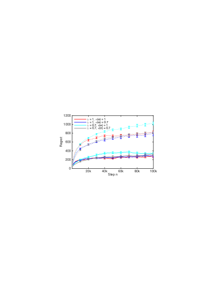
Figure 1: The $n$-step regret of ${\tt CascadeKL\mathchar 45\relax UCB}$ (solid lines) and ${\tt RankedKL\mathchar 45\relax UCB}$ (dotted lines) in the DBN model in Section 5.3.

In our final experiment, we compare ${\tt CascadeKL\mathchar 45\relax UCB}$ to a ranked bandit (Section 6) where the base bandit algorithm is ${\tt KL\mathchar 45\relax UCB}$. We refer to this method as ${\tt RankedKL\mathchar 45\relax UCB}$. The choice of the base algorithm is motivated by the following reasons. First, ${\tt KL\mathchar 45\relax UCB}$ is the best performing oracle in our experiments. Second, since both compared approaches use the same oracle, the difference in their regrets is likely due to their statistical efficiency, and not the oracle itself.

The experimental setup is the same as in Section 5.3. Our results are reported in Figure 1. We observe that the regret of ${\tt RankedKL\mathchar 45\relax UCB}$ is significantly larger than the regret of ${\tt CascadeKL\mathchar 45\relax UCB}$, about three times. The reason is that the regret in ranked bandits is $\Omega(K)$ (Section 6) and $K=4$ in this experiment. The regret of our algorithms is $O(L-K)$ (Section 4.4). Note that ${\tt CascadeKL\mathchar 45\relax UCB}$ is not guaranteed to be optimal in this experiment. Therefore, our results are encouraging and show that ${\tt CascadeKL\mathchar 45\relax UCB}$ could be a viable alternative to more established approaches.

6 Related Work

Ranked bandits are a popular approach in learning to rank (Radlinski et al., 2008) and they are closely related to our work. The key characteristic of ranked bandits is that each position in the recommended list is an independent bandit problem, which is solved by some base bandit algorithm. The solutions in ranked bandits are $(1-1/e)$ approximate and the regret is $\Omega(K)$ (Radlinski et al., 2008), where $K$ is the number of recommended items. Cascading bandits can be viewed as a form of ranked bandits where each recommended item attracts the user independently. We propose novel algorithms for this setting that can learn the optimal solution and whose regret decreases with $K$. We compare one of our algorithms to ranked bandits in Section 5.4.

Our learning problem is of a combinatorial nature, our objective is to learn $K$ most attractive items out of $L$. In this sense, our work is related to stochastic combinatorial bandits, which are often studied with linear rewards and semi-bandit feedback (Gai et al., 2012; Kveton et al., 2014a, b, 2015). The key differences in our work are that the reward function is non-linear in unknown parameters; and that the feedback is less than semi-bandit, only a subset of the recommended items is observed.

Our reward function is non-linear in unknown parameters. These types of problems have been studied before in various contexts. Filippi et al. (2010) proposed and analyzed a generalized linear bandit with bandit feedback. Chen et al. (2013) studied a variant of stochastic combinatorial semi-bandits whose reward function is a known monotone function of a linear function in unknown parameters. Le et al. (2014) studied a network optimization problem whose reward function is a non-linear function of observations.

Bartok et al. (2012) studied finite partial monitoring problems. This is a very general class of problems with finitely many actions, which are chosen by the learning agent; and finitely many outcomes, which are determined by the environment. The outcome is unobserved and must be inferred from the feedback of the environment. Cascading bandits can be viewed as finite partial monitoring problems where the actions are lists of $K$ items out of $L$ and the outcomes are the corners of a $L$-dimensional binary hypercube. Bartok et al. (2012) proposed an algorithm that can solve such problems. This algorithm is computationally inefficient in our problem because it needs to reason over all pairs of actions and stores vectors of length $2^{L}$. Bartok et al. (2012) also do not prove logarithmic distribution-dependent regret bounds as in our work.

Agrawal et al. (1989) studied a partial monitoring problem with non-linear rewards. In this problem, the environment draws a state from a distribution that depends on the action of the learning agent and an unknown parameter. The form of this dependency is known. The state of the environment is observed and determines reward. The reward is a known function of the state and action. Agrawal et al. (1989) also proposed an algorithm for their problem and proved a logarithmic distribution-dependent regret bound. Similarly to Bartok et al. (2012), this algorithm is computationally inefficient in our setting.

Lin et al. (2014) studied partial monitoring in combinatorial bandits. The setting of this work is different from ours. Lin et al. (2014) assume that the feedback is a linear function of the weights of the items that is indexed by actions. Our feedback is a non-linear function of the weights of the items.

Mannor & Shamir (2011) and Caron et al. (2012) studied an opposite setting to ours, where the learning agent observes a superset of chosen items. Chen et al. (2014) studied this problem in stochastic combinatorial semi-bandits.

7 Conclusions

In this paper, we propose a learning variant of the cascade model (Craswell et al., 2008), a popular model of user behavior in web search. We propose two algorithms for solving it, ${\tt CascadeUCB1}$ and ${\tt CascadeKL\mathchar 45\relax UCB}$, and prove gap-dependent upper bounds on their regret. Our analysis addresses two main challenges of our problem, a non-linear reward function and limited feedback. We evaluate our algorithms on several problems and show that they perform well even when our modeling assumptions are violated.

We leave open several questions of interest. For instance, we show in Section 5.3 that ${\tt CascadeKL\mathchar 45\relax UCB}$ can learn the optimal solution to the DBN model. This indicates that the DBN model is learnable in the bandit setting and we leave this for future work. Note that the regret in cascading bandits is $\Omega(L)$ (Section 4.3). Therefore, our learning framework is not practical when the number of items $L$ is large. Similarly to Slivkins et al. (2013), we plan to address this issue by embedding the items in some feature space, along the lines of Wen et al. (2015). Finally, we want to generalize our results to more complex problems, such as learning routing paths in computer networks where the connections fail with unknown probabilities.

From the theoretical point of view, we would like to close the gap between our upper and lower bounds. In addition, we want to derive gap-free bounds. Finally, we would like to refine our analysis so that it explains that the reverse ordering of recommended items yields smaller regret.

Appendix A Proofs of Main Theorems

A.1 Proof of Theorem 2

Let $\mathbf{R}_{t}=R(\mathbf{A}_{t},\mathbf{w}_{t})$ be the regret of the learning algorithm at time $t$, where $\mathbf{A}_{t}$ is the recommended list at time $t$ and $\mathbf{w}_{t}$ are the weights of items at time $t$. Let $\mathcal{E}_{t}=\left\{\exists e\in E\text{ s.t. }\left|\bar{w}(e)-\hat{\mathbf{w}}_{\mathbf{T}_{t-1}(e)}(e)\right|\geq c_{t-1,\mathbf{T}_{t-1}(e)}\right\}$ be the event that $\bar{w}(e)$ is not in the high-probability confidence interval around $\hat{\mathbf{w}}_{\mathbf{T}_{t-1}(e)}(e)$ for some $e$ at time $t$; and let $\overline{\mathcal{E}}_{t}$ be the complement of $\mathcal{E}_{t}$, $\bar{w}(e)$ is in the high-probability confidence interval around $\hat{\mathbf{w}}_{\mathbf{T}_{t-1}(e)}(e)$ for all $e$ at time $t$. Then we can decompose the regret of ${\tt CascadeUCB1}$ as:

$$R(n)=\mathbb{E}\left[\sum_{t=1}^{n}\mathds{1}\!\left\{\mathcal{E}_{t}\right\}\mathbf{R}_{t}\right]+\mathbb{E}\left[\sum_{t=1}^{n}\mathds{1}\!\left\{\overline{\mathcal{E}}_{t}\right\}\mathbf{R}_{t}\right]\,.$$ (10)

Now we bound both terms in the above regret decomposition.

The first term in (10) is small because all of our confidence intervals hold with high probability. In particular, Hoeffding’s inequality (Boucheron et al., 2013, Theorem 2.8) yields that for any $e$, $s$, and $t$:

$$P(\left|\bar{w}(e)-\hat{\mathbf{w}}_{s}(e)\right|\geq c_{t,s})\leq 2\exp[-3\log t]\,,$$

and therefore:

$$\mathbb{E}\left[\sum_{t=1}^{n}\mathds{1}\!\left\{\mathcal{E}_{t}\right\}\right]\leq\sum_{e\in E}\sum_{t=1}^{n}\sum_{s=1}^{t}P(\left|\bar{w}(e)-\hat{\mathbf{w}}_{s}(e)\right|\geq c_{t,s})\leq 2\sum_{e\in E}\sum_{t=1}^{n}\sum_{s=1}^{t}\exp[-3\log t]\leq 2\sum_{e\in E}\sum_{t=1}^{n}t^{-2}\leq\frac{\pi^{2}}{3}L\,.$$

Since $\mathbf{R}_{t}\leq 1$, $\mathbb{E}\left[\sum_{t=1}^{n}\mathds{1}\!\left\{\mathcal{E}_{t}\right\}\mathbf{R}_{t}\right]\leq\frac{\pi^{2}}{3}L$.

Recall that $\mathbb{E}_{t}\left[\cdot\right]=\mathbb{E}\left[\cdot\,\middle|\,\mathcal{H}_{t}\right]$, where $\mathcal{H}_{t}$ is the history of the learning agent up to choosing $\mathbf{A}_{t}$, the first $t-1$ observations and $t$ actions (4). Based on this definition, we rewrite the second term in (10) as:

$$\mathbb{E}\left[\sum_{t=1}^{n}\mathds{1}\!\left\{\overline{\mathcal{E}}_{t}\right\}\mathbf{R}_{t}\right]\stackrel{{\scriptstyle\text{(a)}}}{{=}}\sum_{t=1}^{n}\mathbb{E}\left[\mathds{1}\!\left\{\overline{\mathcal{E}}_{t}\right\}\mathbb{E}_{t}\left[\mathbf{R}_{t}\right]\right]\stackrel{{\scriptstyle\text{(b)}}}{{\leq}}\sum_{e=K+1}^{L}\mathbb{E}\left[\sum_{e^{\ast}=1}^{K}\sum_{t=1}^{n}\Delta_{e,e^{\ast}}\mathds{1}\!\left\{\overline{\mathcal{E}}_{t},G_{e,e^{\ast},t}\right\}\right]\,,$$

where equality (a) is due to the tower rule and that $\mathds{1}\!\left\{\overline{\mathcal{E}}_{t}\right\}$ is only a function of $\mathcal{H}_{t}$, and inequality (b) is due to the upper bound in Theorem 1.

Now we bound $\sum_{e^{\ast}=1}^{K}\sum_{t=1}^{n}\Delta_{e,e^{\ast}}\mathds{1}\!\left\{\overline{\mathcal{E}}_{t},G_{e,e^{\ast},t}\right\}$ for any suboptimal item $e$. Select any optimal item $e^{\ast}$. When event $\overline{\mathcal{E}}_{t}$ happens, $\left|\bar{w}(e)-\hat{\mathbf{w}}_{\mathbf{T}_{t-1}(e)}(e)\right|<c_{t-1,\mathbf{T}_{t-1}(e)}$. Moreover, when event $G_{e,e^{\ast},t}$ happens, $\mathbf{U}_{t}(e)\geq\mathbf{U}_{t}(e^{\ast})$ by Theorem 1. Therefore, when both $G_{e,e^{\ast},t}$ and $\overline{\mathcal{E}}_{t}$ happen:

$$\bar{w}(e)+2c_{t-1,\mathbf{T}_{t-1}(e)}\geq\mathbf{U}_{t}(e)\geq\mathbf{U}_{t}(e^{\ast})\geq\bar{w}(e^{\ast})\,,$$

which implies:

$$2c_{t-1,\mathbf{T}_{t-1}(e)}\geq\Delta_{e,e^{\ast}}\,.$$

Together with $c_{n,\mathbf{T}_{t-1}(e)}\geq c_{t-1,\mathbf{T}_{t-1}(e)}$, this implies $\mathbf{T}_{t-1}(e)\leq\tau_{e,e^{\ast}}$, where $\tau_{e,e^{\ast}}=\frac{6}{\Delta_{e,e^{\ast}}^{2}}\log n$. Therefore:

$$\sum_{e^{\ast}=1}^{K}\sum_{t=1}^{n}\Delta_{e,e^{\ast}}\mathds{1}\!\left\{\overline{\mathcal{E}}_{t},G_{e,e^{\ast},t}\right\}\leq\sum_{e^{\ast}=1}^{K}\Delta_{e,e^{\ast}}\sum_{t=1}^{n}\mathds{1}\!\left\{\mathbf{T}_{t-1}(e)\leq\tau_{e,e^{\ast}},\ G_{e,e^{\ast},t}\right\}\,.$$ (11)

Let:

$$\mathbf{M}_{e,e^{\ast}}=\sum_{t=1}^{n}\mathds{1}\!\left\{\mathbf{T}_{t-1}(e)\leq\tau_{e,e^{\ast}},\ G_{e,e^{\ast},t}\right\}$$

be the inner sum in (11). Now note that (i) the counter $\mathbf{T}_{t-1}(e)$ of item $e$ increases by one when the event $G_{e,e^{\ast},t}$ happens for any optimal item $e^{\ast}$, (ii) the event $G_{e,e^{\ast},t}$ happens for at most one optimal $e^{\ast}$ at any time $t$; and (iii) $\tau_{e,1}\leq\ldots\leq\tau_{e,K}$. Based on these facts, it follows that $\mathbf{M}_{e,e^{\ast}}\leq\tau_{e,e^{\ast}}$, and moreover $\sum_{e^{\ast}=1}^{K}\mathbf{M}_{e,e^{\ast}}\leq\tau_{e,K}$. Therefore, the right-hand side of (11) can be bounded from above by:

$$\max\left\{\sum_{e^{\ast}=1}^{K}\Delta_{e,e^{\ast}}m_{e,e^{\ast}}:0\leq m_{e,e^{\ast}}\leq\tau_{e,e^{\ast}},\ \sum_{e^{\ast}=1}^{K}m_{e,e^{\ast}}\leq\tau_{e,K}\right\}\,.$$

Since the gaps are decreasing, $\Delta_{e,1}\geq\ldots\geq\Delta_{e,K}$, the solution to the above problem is $m_{e,1}^{\ast}=\tau_{e,1}$, $m_{e,2}^{\ast}=\tau_{e,2}-\tau_{e,1}$, $\dots$, $m_{e,K}^{\ast}=\tau_{e,K}-\tau_{e,K-1}$. Therefore, the value of (11) is bounded from above by:

$$\left[\Delta_{e,1}\frac{1}{\Delta_{e,1}^{2}}+\sum_{e^{\ast}=2}^{K}\Delta_{e,e^{\ast}}\left(\frac{1}{\Delta_{e,e^{\ast}}^{2}}-\frac{1}{\Delta_{e,e^{\ast}-1}^{2}}\right)\right]6\log n\,.$$

By Lemma 3 of Kveton et al. (2014a), the above term is bounded by $\frac{12}{\Delta_{e,K}}\log n$. Finally, we chain all inequalities and sum over all suboptimal items $e$.

A.2 Proof of Theorem 3

Let $\mathbf{R}_{t}=R(\mathbf{A}_{t},\mathbf{w}_{t})$ be the regret of the learning algorithm at time $t$, where $\mathbf{A}_{t}$ is the recommended list at time $t$ and $\mathbf{w}_{t}$ are the weights of items at time $t$. Let $\mathcal{E}_{t}=\left\{\exists 1\leq e\leq K\text{ s.t. }\bar{w}(e)>\mathbf{U}_{t}(e)\right\}$ be the event that the attraction probability of at least one optimal item is above its upper confidence bound at time $t$. Let $\overline{\mathcal{E}}_{t}$ be the complement of event $\mathcal{E}_{t}$. Then we can decompose the regret of ${\tt CascadeKL\mathchar 45\relax UCB}$ as:

$$R(n)=\mathbb{E}\left[\sum_{t=1}^{n}\mathds{1}\!\left\{\mathcal{E}_{t}\right\}\mathbf{R}_{t}\right]+\mathbb{E}\left[\sum_{t=1}^{n}\mathds{1}\!\left\{\overline{\mathcal{E}}_{t}\right\}\mathbf{R}_{t}\right]\,.$$ (12)

By Theorems 2 and 10 of Garivier & Cappe (2011), thanks to the choice of the upper confidence bound $\mathbf{U}_{t}$, the first term in (12) is bounded as $\mathbb{E}\left[\sum_{t=1}^{n}\mathds{1}\!\left\{\mathcal{E}_{t}\right\}\mathbf{R}_{t}\right]\leq 7K\log\log n$. As in the proof of Theorem 2, we rewrite the second term as:

$$\mathbb{E}\left[\sum_{t=1}^{n}\mathds{1}\!\left\{\overline{\mathcal{E}}_{t}\right\}\mathbf{R}_{t}\right]=\sum_{t=1}^{n}\mathbb{E}\left[\mathds{1}\!\left\{\overline{\mathcal{E}}_{t}\right\}\mathbb{E}_{t}\left[\mathbf{R}_{t}\right]\right]\leq\sum_{e=K+1}^{L}\mathbb{E}\left[\sum_{e^{\ast}=1}^{K}\sum_{t=1}^{n}\Delta_{e,e^{\ast}}\mathds{1}\!\left\{\overline{\mathcal{E}}_{t},G_{e,e^{\ast},t}\right\}\right]\,.$$

Now note that for any suboptimal item $e$ and $\tau_{e,e^{\ast}}>0$:

$$\mathbb{E}\left[\sum_{e^{\ast}=1}^{K}\sum_{t=1}^{n}\Delta_{e,e^{\ast}}\mathds{1}\!\left\{\overline{\mathcal{E}}_{t},G_{e,e^{\ast},t}\right\}\right] \leq\mathbb{E}\left[\sum_{e^{\ast}=1}^{K}\sum_{t=1}^{n}\Delta_{e,e^{\ast}}\mathds{1}\!\left\{\mathbf{T}_{t-1}(e)\leq\tau_{e,e^{\ast}},\ G_{e,e^{\ast},t}\right\}\right]+{}$$ (13)

$$\phantom{{}={}}\sum_{e^{\ast}=1}^{K}\Delta_{e,e^{\ast}}\mathbb{E}\left[\sum_{t=1}^{n}\mathds{1}\!\left\{\mathbf{T}_{t-1}(e)>\tau_{e,e^{\ast}},\ \overline{\mathcal{E}}_{t},\ G_{e,e^{\ast},t}\right\}\right]\,.$$

Let:

$$\tau_{e,e^{\ast}}=\frac{1+\varepsilon}{D_{\mathrm{KL}}(\bar{w}(e)\,\|\,\bar{w}(e^{\ast}))}(\log n+3\log\log n)\,.$$

Then by the same argument as in Theorem 2 and Lemma 8 of Garivier & Cappe (2011):

$$\mathbb{E}\left[\sum_{t=1}^{n}\mathds{1}\!\left\{\mathbf{T}_{t-1}(e)>\tau_{e,e^{\ast}},\ \overline{\mathcal{E}}_{t},\ G_{e,e^{\ast},t}\right\}\right]\leq\frac{C_{2}(\varepsilon)}{n^{\beta(\varepsilon)}}$$

holds for any suboptimal $e$ and optimal $e^{\ast}$. So the second term in (13) is bounded from above by $K\frac{C_{2}(\varepsilon)}{n^{\beta(\varepsilon)}}$. Now we bound the first term in (13). By the same argument as in the proof of Theorem 2:

$$\sum_{e^{\ast}=1}^{K}\sum_{t=1}^{n}\Delta_{e,e^{\ast}}\mathds{1}\!\left\{\mathbf{T}_{t-1}(e)\leq\tau_{e,e^{\ast}},\ G_{e,e^{\ast},t}\right\}\leq$$

$$\quad\left[\frac{\Delta_{e,1}}{D_{\mathrm{KL}}(\bar{w}(e)\,\|\,\bar{w}(1))}+\sum_{e^{\ast}=2}^{K}\Delta_{e,e^{\ast}}\left(\frac{1}{D_{\mathrm{KL}}(\bar{w}(e)\,\|\,\bar{w}(e^{\ast}))}-\frac{1}{D_{\mathrm{KL}}(\bar{w}(e)\,\|\,\bar{w}(e^{\ast}-1))}\right)\right](1+\varepsilon)(\log n+3\log\log n)$$

holds for any suboptimal item $e$. By Lemma 2, the leading constant is bounded as:

$$\frac{\Delta_{e,1}}{D_{\mathrm{KL}}(\bar{w}(e)\,\|\,\bar{w}(1))}+\sum_{e^{\ast}=2}^{K}\Delta_{e,e^{\ast}}\left(\frac{1}{D_{\mathrm{KL}}(\bar{w}(e)\,\|\,\bar{w}(e^{\ast}))}-\frac{1}{D_{\mathrm{KL}}(\bar{w}(e)\,\|\,\bar{w}(e^{\ast}-1))}\right)\leq\frac{\Delta_{e,K}(1+\log(1/\Delta_{e,K}))}{D_{\mathrm{KL}}(\bar{w}(e)\,\|\,\bar{w}(K))}\,.$$

Finally, we chain all inequalities and sum over all suboptimal items $e$.

Appendix B Technical Lemmas

Lemma 1.

Let $A=(a_{1},\dots,a_{K})$ and $B=(b_{1},\dots,b_{K})$ be any two lists of $K$ items from $\Pi_{K}(E)$ such that $a_{i}=b_{j}$ only if $i=j$. Let $\mathbf{w}\sim P$ in 1. Then:

$$\mathbb{E}\left[\prod_{k=1}^{K}\mathbf{w}(a_{k})-\prod_{k=1}^{K}\mathbf{w}(b_{k})\right]=\sum_{k=1}^{K}\mathbb{E}\left[\prod_{i=1}^{k-1}\mathbf{w}(a_{i})\right]\mathbb{E}\left[\mathbf{w}(a_{k})-\mathbf{w}(b_{k})\right]\left(\prod_{j=k+1}^{K}\mathbb{E}\left[\mathbf{w}(b_{j})\right]\right)\,.$$

Proof.

First, we prove that:

$$\prod_{k=1}^{K}w(a_{k})-\prod_{k=1}^{K}w(b_{k})=\sum_{k=1}^{K}\left(\prod_{i=1}^{k-1}w(a_{i})\right)(w(a_{k})-w(b_{k}))\left(\prod_{j=k+1}^{K}w(b_{j})\right)$$

holds for any $w\in\left\{0,1\right\}^{L}$. The proof is by induction on $K$. The claim holds obviously for $K=1$. Now suppose that the claim holds for any $A,B\in\Pi_{K-1}(E)$. Let $A,B\in\Pi_{K}(E)$. Then:

$$\prod_{k=1}^{K}w(a_{k})-\prod_{k=1}^{K}w(b_{k}) =\prod_{k=1}^{K}w(a_{k})-w(b_{K})\prod_{k=1}^{K-1}w(a_{k})+w(b_{K})\prod_{k=1}^{K-1}w(a_{k})-\prod_{k=1}^{K}w(b_{k})$$

$$=(w(a_{K})-w(b_{K}))\prod_{k=1}^{K-1}w(a_{k})+w(b_{K})\left[\prod_{k=1}^{K-1}w(a_{k})-\prod_{k=1}^{K-1}w(b_{k})\right]$$

$$=(w(a_{K})-w(b_{K}))\prod_{k=1}^{K-1}w(a_{k})+\sum_{k=1}^{K-1}\left(\prod_{i=1}^{k-1}w(a_{i})\right)(w(a_{k})-w(b_{k}))\left(\prod_{j=k+1}^{K}w(b_{j})\right)$$

$$=\sum_{k=1}^{K}\left(\prod_{i=1}^{k-1}w(a_{i})\right)(w(a_{k})-w(b_{k}))\left(\prod_{j=k+1}^{K}w(b_{j})\right)\,.$$

The third equality is by our induction hypothesis. Finally, note that $\mathbf{w}$ is drawn from a factored distribution. Therefore, we can decompose the expectation of the product as a product of expectations, and our claim follows.  

Lemma 2.

Let $p_{1}\geq\ldots\geq p_{K}>p$ be $K+1$ probabilities and $\Delta_{k}=p_{k}-p$ for $1\leq k\leq K$. Then:

$$\frac{\Delta_{1}}{D_{\mathrm{KL}}(p\,\|\,p_{1})}+\sum_{k=2}^{K}\Delta_{k}\left(\frac{1}{D_{\mathrm{KL}}(p\,\|\,p_{k})}-\frac{1}{D_{\mathrm{KL}}(p\,\|\,p_{k-1})}\right)\leq\frac{\Delta_{K}(1+\log(1/\Delta_{K}))}{D_{\mathrm{KL}}(p\,\|\,p_{K})}\,.$$

Proof.

First, we note that:

$$\frac{\Delta_{1}}{D_{\mathrm{KL}}(p\,\|\,p_{1})}+\sum_{k=2}^{K}\Delta_{k}\left(\frac{1}{D_{\mathrm{KL}}(p\,\|\,p_{k})}-\frac{1}{D_{\mathrm{KL}}(p\,\|\,p_{k-1})}\right)=\sum_{k=1}^{K-1}\frac{\Delta_{k}-\Delta_{k+1}}{D_{\mathrm{KL}}(p\,\|\,p_{k})}+\frac{\Delta_{K}}{D_{\mathrm{KL}}(p\,\|\,p_{K})}\,.$$

The summation over $k$ can be bounded from above by a definite integral:

$$\sum_{k=1}^{K-1}\frac{\Delta_{k}-\Delta_{k+1}}{D_{\mathrm{KL}}(p\,\|\,p_{k})}=\sum_{k=1}^{K-1}\frac{\Delta_{k}-\Delta_{k+1}}{D_{\mathrm{KL}}(p\,\|\,p+\Delta_{k})}\leq\int_{\Delta_{K}}^{\Delta_{1}}\frac{1}{D_{\mathrm{KL}}(p\,\|\,p+x)}\,\mathrm{d}x\leq\int_{\Delta_{K}}^{1}\frac{1}{D_{\mathrm{KL}}(p\,\|\,p+x)}\,\mathrm{d}x\,,$$

where the first inequality follows from the fact that $1/D_{\mathrm{KL}}(p\,\|\,p+x)$ decreases on $x\geq 0$. To the best of our knowledge, the integral of $1/D_{\mathrm{KL}}(p\,\|\,p+x)$ over $x$ does not have a simple analytic solution. Therefore, we integrate an upper bound on $1/D_{\mathrm{KL}}(p\,\|\,p+x)$ which does. In particular, note that for any $x\geq\Delta_{K}$:

$$D_{\mathrm{KL}}(p\,\|\,p+x)\geq\frac{D_{\mathrm{KL}}(p\,\|\,p+\Delta_{K})}{\Delta_{K}}x=\frac{D_{\mathrm{KL}}(p\,\|\,p_{K})}{\Delta_{K}}x$$

because $D_{\mathrm{KL}}(p\,\|\,p+x)$ is convex, increasing in $x\geq 0$, and its minimum is attained at $x=0$. Therefore:

$$\int_{\Delta_{K}}^{1}\frac{1}{D_{\mathrm{KL}}(p\,\|\,p+x)}\,\mathrm{d}x\leq\frac{\Delta_{K}}{D_{\mathrm{KL}}(p\,\|\,p_{K})}\int_{\Delta_{K}}^{1}\frac{1}{x}\,\mathrm{d}x=\frac{\Delta_{K}}{D_{\mathrm{KL}}(p\,\|\,p_{K})}\log(1/\Delta_{K})\,.$$

Finally, we chain all inequalities and get the final result.

References

- Agichtein et al. (2006) Agichtein, Eugene, Brill, Eric, and Dumais, Susan. Improving web search ranking by incorporating user behavior information. In Proceedings of the 29th Annual International ACM SIGIR Conference, pp. 19–26, 2006.
- Agrawal et al. (1989) Agrawal, Rajeev, Teneketzis, Demosthenis, and Anantharam, Venkatachalam. Asymptotically efficient adaptive allocation schemes for controlled i.i.d. processes: Finite parameter space. IEEE Transactions on Automatic Control, 34(3):258–267, 1989.
- Auer et al. (2002) Auer, Peter, Cesa-Bianchi, Nicolo, and Fischer, Paul. Finite-time analysis of the multiarmed bandit problem. Machine Learning, 47:235–256, 2002.
- Bartok et al. (2012) Bartok, Gabor, Zolghadr, Navid, and Szepesvari, Csaba. An adaptive algorithm for finite stochastic partial monitoring. In Proceedings of the 29th International Conference on Machine Learning, 2012.
- Becker et al. (2007) Becker, Hila, Meek, Christopher, and Chickering, David Maxwell. Modeling contextual factors of click rates. In Proceedings of the 22nd AAAI Conference on Artificial Intelligence, pp. 1310–1315, 2007.
- Boucheron et al. (2013) Boucheron, Stephane, Lugosi, Gabor, and Massart, Pascal. Concentration Inequalities: A Nonasymptotic Theory of Independence. Oxford University Press, 2013.
- Caron et al. (2012) Caron, Stephane, Kveton, Branislav, Lelarge, Marc, and Bhagat, Smriti. Leveraging side observations in stochastic bandits. In Proceedings of the 28th Conference on Uncertainty in Artificial Intelligence, pp. 142–151, 2012.
- Chapelle & Zhang (2009) Chapelle, Olivier and Zhang, Ya. A dynamic bayesian network click model for web search ranking. In Proceedings of the 18th International Conference on World Wide Web, pp. 1–10, 2009.
- Chen et al. (2013) Chen, Wei, Wang, Yajun, and Yuan, Yang. Combinatorial multi-armed bandit: General framework, results and applications. In Proceedings of the 30th International Conference on Machine Learning, pp. 151–159, 2013.
- Chen et al. (2014) Chen, Wei, Wang, Yajun, and Yuan, Yang. Combinatorial multi-armed bandit and its extension to probabilistically triggered arms. CoRR, abs/1407.8339, 2014.
- Craswell et al. (2008) Craswell, Nick, Zoeter, Onno, Taylor, Michael, and Ramsey, Bill. An experimental comparison of click position-bias models. In Proceedings of the 1st ACM International Conference on Web Search and Data Mining, pp. 87–94, 2008.
- Filippi et al. (2010) Filippi, Sarah, Cappe, Olivier, Garivier, Aurelien, and Szepesvari, Csaba. Parametric bandits: The generalized linear case. In Advances in Neural Information Processing Systems 23, pp. 586–594, 2010.
- Gai et al. (2012) Gai, Yi, Krishnamachari, Bhaskar, and Jain, Rahul. Combinatorial network optimization with unknown variables: Multi-armed bandits with linear rewards and individual observations. IEEE/ACM Transactions on Networking, 20(5):1466–1478, 2012.
- Garivier & Cappe (2011) Garivier, Aurelien and Cappe, Olivier. The KL-UCB algorithm for bounded stochastic bandits and beyond. In Proceeding of the 24th Annual Conference on Learning Theory, pp. 359–376, 2011.
- Guo et al. (2009a) Guo, Fan, Liu, Chao, Kannan, Anitha, Minka, Tom, Taylor, Michael, Wang, Yi Min, and Faloutsos, Christos. Click chain model in web search. In Proceedings of the 18th International Conference on World Wide Web, pp. 11–20, 2009a.
- Guo et al. (2009b) Guo, Fan, Liu, Chao, and Wang, Yi Min. Efficient multiple-click models in web search. In Proceedings of the 2nd ACM International Conference on Web Search and Data Mining, pp. 124–131, 2009b.
- Kveton et al. (2014a) Kveton, Branislav, Wen, Zheng, Ashkan, Azin, Eydgahi, Hoda, and Eriksson, Brian. Matroid bandits: Fast combinatorial optimization with learning. In Proceedings of the 30th Conference on Uncertainty in Artificial Intelligence, pp. 420–429, 2014a.
- Kveton et al. (2014b) Kveton, Branislav, Wen, Zheng, Ashkan, Azin, and Valko, Michal. Learning to act greedily: Polymatroid semi-bandits. CoRR, abs/1405.7752, 2014b.
- Kveton et al. (2015) Kveton, Branislav, Wen, Zheng, Ashkan, Azin, and Szepesvari, Csaba. Tight regret bounds for stochastic combinatorial semi-bandits. In Proceedings of the 18th International Conference on Artificial Intelligence and Statistics, 2015.
- Lai & Robbins (1985) Lai, T. L. and Robbins, Herbert. Asymptotically efficient adaptive allocation rules. Advances in Applied Mathematics, 6(1):4–22, 1985.
- Le et al. (2014) Le, Thanh, Szepesvari, Csaba, and Zheng, Rong. Sequential learning for multi-channel wireless network monitoring with channel switching costs. IEEE Transactions on Signal Processing, 62(22):5919–5929, 2014.
- Lin et al. (2014) Lin, Tian, Abrahao, Bruno, Kleinberg, Robert, Lui, John, and Chen, Wei. Combinatorial partial monitoring game with linear feedback and its applications. In Proceedings of the 31st International Conference on Machine Learning, pp. 901–909, 2014.
- Mannor & Shamir (2011) Mannor, Shie and Shamir, Ohad. From bandits to experts: On the value of side-observations. In Advances in Neural Information Processing Systems 24, pp. 684–692, 2011.
- Radlinski & Joachims (2005) Radlinski, Filip and Joachims, Thorsten. Query chains: Learning to rank from implicit feedback. In Proceedings of the 11th ACM SIGKDD International Conference on Knowledge Discovery and Data Mining, pp. 239–248, 2005.
- Radlinski et al. (2008) Radlinski, Filip, Kleinberg, Robert, and Joachims, Thorsten. Learning diverse rankings with multi-armed bandits. In Proceedings of the 25th International Conference on Machine Learning, pp. 784–791, 2008.
- Richardson et al. (2007) Richardson, Matthew, Dominowska, Ewa, and Ragno, Robert. Predicting clicks: Estimating the click-through rate for new ads. In Proceedings of the 16th International Conference on World Wide Web, pp. 521–530, 2007.
- Slivkins et al. (2013) Slivkins, Aleksandrs, Radlinski, Filip, and Gollapudi, Sreenivas. Ranked bandits in metric spaces: Learning diverse rankings over large document collections. Journal of Machine Learning Research, 14(1):399–436, 2013.
- Wen et al. (2015) Wen, Zheng, Kveton, Branislav, and Ashkan, Azin. Efficient learning in large-scale combinatorial semi-bandits. In Proceedings of the 32nd International Conference on Machine Learning, 2015.