Numerical Study of the Longitudinally Asymmetric Distribution of Solar Energetic Particles in the Heliosphere

Abstract

Solar energetic particles (SEPs) affect the solar-terrestrial space environment and become a very important aspect in space weather research. In this work, we numerically investigate the transport processes of SEPs in three-dimensional interplanetary magnetic field, with an emphasis on the longitudinal distribution of SEPs in the heliosphere. We confirm our previous finding that there exists an east-west longitudinal asymmetry in the SEP intensities, i.e., with the same longitude separations between the solar source centers and the magnetic footpoint of the observer, the fluxes of SEP events originating from solar sources located on the eastern side of the nominal magnetic footpoint of the observer are systematically larger than those of the SEP events originating from sources located on the western side. We discuss the formation mechanism of this phenomenon, and conclude that the longitudinally asymmetric distribution of SEPs results from the east-west azimuthal asymmetry in the topology of the heliospheric magnetic field as well as the effects of perpendicular diffusion on the transport of SEPs in the heliosphere. Our results will be valuable to understanding Sun-Earth relations and useful for space weather forecasting.

1 Introduction

Solar energetic particles (SEPs), which are charged energetic particles occasionally emitted by the Sun, risk the health of astronauts working in space and damage electronic components on satellites, so they have become a very important aspect affecting solar-terrestrial space environment and space weather. Theoretically, SEPs observed in the interplanetary magnetic field provide fundamental information regarding the acceleration mechanisms and transport processes of charged energetic particles. Therefore, the subject has become a focus of astrophysics, space physics, and plasma physics.

Through several decades of investigations in the community with spacecraft observations and theoretical modeling, significant progresses have been achieved toward a better understanding of the transport processes of SEPs. As a pioneering work, Parker (1965) provided a diffusion equation to investigate the modulation of galactic cosmic rays and the transport of SEPs. It is very difficult to analytically solve the multidimensional transport equation; consequently, numerical calculations are usually adopted (e.g., Ng & Wong, 1979; Ruffolo, 1991; Zhang et al., 2009; He & Qin, 2011; He et al., 2011; Giacalone & Jokipii, 2012). Jokipii (1966) proposed the well-known and classical quasi-linear theory (QLT) to describe the diffusion of charged particles in a turbulent magnetic field. The theoretical investigations and observational analyses based on SEP events measured by the Helios spacecraft suggested some nonlinear effects near $90^{\circ}$ pitch angle in the particle pitch-angle distributions (e.g., Hasselmann & Wibberenz, 1968, 1970; Beeck & Wibberenz, 1986; Beeck et al., 1987). Schlickeiser (2002) laid complete physical foundations and presented profound mathematical techniques for cosmic ray transport research. Matthaeus et al. (2003) provided a nonlinear guiding center (NLGC) theory for charged particles’ perpendicular diffusion to account for the numerical simulation results of test particles. Shalchi et al. (2004) presented analytical forms for the results from the NLGC theory. Zank et al. (2000) and Li et al. (2003) provided a dynamical time-dependent model of charged particle acceleration at a propagating and evolving interplanetary shock.

Recently, Zhang et al. (2009) presented a model calculation of SEP propagation in a three-dimensional interplanetary magnetic field with the effect of magnetic turbulence. He et al. (2011) investigated the effects of particle source characteristics on SEP observations at 1 AU and found that the perpendicular diffusion has a very important influence on the propagation of SEPs in the heliosphere, particularly when a spacecraft is not directly connected to the acceleration regions either on the Sun or near the CME-driven shocks by the interplanetary magnetic field lines; in such cases, the earliest arriving particles can be seen propagating toward the Sun, having scattered backward at large distances. He & Wan (2012a) presented a direct method to quickly and explicitly determine the spatially dependent parallel and radial mean free paths of SEPs with adiabatic focusing. Furthermore, He & Wan (2012b) provided a direct approach to explicitly investigate the spatially dependent perpendicular mean free path of SEPs in a turbulent and spatially varying magnetic field. They reported that for physical conditions representative of the solar wind and the magnetic turbulence, the ratio $\lambda_{\perp}/\lambda_{\parallel}$ of the perpendicular to the parallel mean free path remains in the range $0.01-0.20$; however, when the turbulence strength $\delta B/B$ is sufficiently large, the ratio $\lambda_{\perp}/\lambda_{\parallel}$ would approach or exceed unity.

Observationally, Cane et al. (1988) investigated time profiles of 235 intense proton events to document the longitude-dependent profiles. Reames (1999) presented some observational evidences of longitudinal effects on the transport processes of SEPs. They found that the interplanetary spiral magnetic field causes an asymmetry in the intensity time profiles of SEP events originating from eastern and western longitudes on the solar disk. As we know, SEPs are usually produced by solar flares or/and related to coronal mass ejections (CMEs) (e.g., Reames, 1999). Recently, Dresing et al. (2012) investigated in detail the large longitudinal spread of SEPs during the 17 January 2010 solar event and suggested with observational evidence that the wide longitudinal spread of particles is mainly due to perpendicular diffusion in the interplanetary medium.

In He et al. (2011), the authors found that with the same separation in heliographic longitude between the magnetic footpoint of the observer and the solar sources, the SEPs associated with the sources located east are detected earlier with larger fluxes than those associated with the sources located west. This interesting phenomenon was called the “east-west azimuthal asymmetry of SEPs” by He et al. (2011). The simulation results in Giacalone & Jokipii (2012) also showed similar asymmetric features of SEP distribution. In this paper, we focus on the so-called east-west azimuthal asymmetry of SEPs in view of numerical investigations. There are several previous works studying the longitudinal dependence of SEP intensities (e.g., Cane et al., 1988; Reames, 1999). Basically, however, these previous studies only analyzed the effects of heliographic longitude of particle sources on the intensity profiles of SEP events. In our simulations, we mainly investigate the relatively longitudinal distribution of SEP intensities in the heliosphere, and find the longitudinally asymmetric distribution phenomenon. With the same longitude separations between the solar source centers and the magnetic field line footpoint of the observer, the fluxes of SEP events originating from solar sources located on the eastern side of the nominal magnetic footpoint of observer are systematically larger than those of the SEP events originating from sources located on the western side. We conclude that the longitudinally asymmetric distribution of SEPs results from the east-west azimuthal asymmetry in the geometry of the heliospheric magnetic field as well as the effects of perpendicular diffusion on the transport processes of SEPs in the heliosphere. Our results will be valuable for understanding solar-terrestrial relations and useful in space weather forecasting. Some investigation results related with the statistical and numerical studies on the longitudinally asymmetric distribution of SEPs were reported in the 33rd International Cosmic Ray Conference (He & Wan, 2013a).

This paper is organized as follows. Firstly, in Section 2, we present a five-dimensional focussed transport model containing most of the usually used transport mechanisms. The simulation method for numerically solving the focussed transport equation is also provided in this section. In Section 3, the simulation results of the relatively longitudinal distribution of SEPs will be presented. We present some implications of our simulation results in Section 4 and a discussion on the formation mechanism in Section 5. A summary of our results will be provided in Section 6.

2 Numerical Model and Method

In our model, the five-dimensional focussed transport equation that governs the gyrophase-averaged distribution function $f(\textbf{x},\mu,p,t)$ of SEPs can be written as (e.g., Schlickeiser, 2002; Zhang et al., 2009; He et al., 2011; Qin et al., 2011)

$$\frac{\partial f}{\partial t}+\mu v\frac{\partial f}{\partial z}+{\bf V}^{sw}\cdot\nabla f+\frac{dp}{dt}\frac{\partial f}{\partial p}+\frac{d\mu}{dt}\frac{\partial f}{\partial\mu}$$

$$-\frac{\partial}{\partial\mu}\left(D_{\mu\mu}\frac{\partial f}{\partial\mu}\right)-\frac{\partial}{\partial x}\bigg{(}\kappa_{xx}\frac{\partial f}{\partial x}\bigg{)}-\frac{\partial}{\partial y}\left(\kappa_{yy}\frac{\partial f}{\partial y}\right)=Q({\bf x},p,t),$$ (1)

where x is particle’s position, $z$ is the coordinate along the magnetic field spiral, $p$ is particle’s momentum, $\mu$ is the pitch-angle cosine of particle, $t$ is time, $v$ is the particle velocity, $\textbf{V}^{sw}$ is the solar wind speed, and $Q$ is the source term. In the transport model, we directly input a source of accelerated particles as a product of either a solar flare or the CME-driven shock. We focus on the high-energy SEPs accelerated and released into the system near the Sun. The particle injection can be seen as a point source in the radial direction. For observations far out near 1 AU or larger radial distances, this assumption is particularly valid and is commonly used in the study of SEP transport (e.g., Zhang et al., 2009). The particle momentum change term $dp/dt$ in Equation (1) due to the adiabatic cooling effect can be written as (Skilling, 1971)

$$\frac{dp}{dt}=-p\left[\frac{1-\mu^{2}}{2}\left(\frac{\partial V^{sw}_{x}}{\partial x}+\frac{\partial V^{sw}_{y}}{\partial y}\right)+\mu^{2}\frac{\partial V^{sw}_{z}}{\partial z}\right].$$ (2)

In addition, $d\mu/dt$, which includes the magnetic focusing effect and the divergence of the solar wind flows effect, can be expressed as (e.g., Roelof, 1969; Isenberg, 1997; Kóta & Jokipii, 1997)

$$\frac{d\mu}{dt} = \frac{1-\mu^{2}}{2}\left[-\frac{v}{B}\frac{\partial B}{\partial z}+\mu\left(\frac{\partial V^{sw}_{x}}{\partial x}+\frac{\partial V^{sw}_{y}}{\partial y}-2\frac{\partial V^{sw}_{z}}{\partial z}\right)\right]$$ (3)

$$= \frac{1-\mu^{2}}{2}\left[\frac{v}{L}+\mu\left(\frac{\partial V^{sw}_{x}}{\partial x}+\frac{\partial V^{sw}_{y}}{\partial y}-2\frac{\partial V^{sw}_{z}}{\partial z}\right)\right],$$

where $B$ is the background interplanetary magnetic field with direction z, and the magnetic focusing length $L$ is defined as $L=(\textbf{z}\cdot\bigtriangledown\ln B)^{-1}$. Therefore, the adiabatic cooling effect and the divergence of the solar wind flows effect generated by the solar wind velocity components, expressed as Equations (2) and (3), respectively, have been included in our model. The interplanetary magnetic field in the inner heliosphere is too strong and the particle energies in typical SEP events are not high enough, so in this work we neglect the particle drift in the nonuniform magnetic field (Zhang et al., 2009).

Under the diffusion approximation for a nearly isotropic pitch-angle distribution, the parallel mean free path $\lambda_{\parallel}$ can be written as (Jokipii, 1966; Hasselmann & Wibberenz, 1968; Earl, 1974; He & Schlickeiser, 2014)

$$\lambda_{\parallel}=\frac{3v}{8}\int_{-1}^{+1}\frac{(1-\mu^{2})^{2}}{D_{\mu\mu}}d\mu.$$ (4)

Accordingly, the radial mean free path can be defined as

$$\lambda_{r}=\lambda_{\parallel}\cos^{2}\psi,$$ (5)

where $\psi$ is the angle between the local magnetic field direction and the radial direction. In Equation (5), $\cos^{2}\psi$ can be written as (Ng & Gleeson, 1971; He & Wan, 2012a)

$$\cos^{2}\psi=(V^{sw})^{2}/\left((V^{sw})^{2}+\Omega^{2}r^{2}\sin^{2}\theta\right),$$ (6)

where $V^{sw}$ is the solar wind speed, $\Omega$ is the angular rotation velocity of the Sun, and $r$ and $\theta$ are the coordinates of the heliocentric spherical coordinate system $(r,\theta,\phi)$, namely, $r$ is the heliocentric radial distance, and $\theta$ is the colatitude, which is measured from the rotation axis of the Sun.

We use a form of the pitch-angle diffusion coefficient as (e.g., Beeck & Wibberenz, 1986; He et al., 2011)

$$D_{\mu\mu}^{r}=D_{\mu\mu}/\cos^{2}\psi=D_{0}vR^{-1/3}\left(|\mu|^{q-1}+h\right)(1-\mu^{2}),$$ (7)

where $D_{0}$ is a constant indicating the magnetic turbulence strength and $R$ is the particle rigidity. The constant $h$ is needed to simulate the particles’ ability to scatter through $\mu=0$. In order to simulate the nonlinear effect to cause large $D_{\mu\mu}$ at $\mu=0$, we use a relatively large value of $h=0.2$. The constant $q$ is related to the power spectrum of the magnetic field turbulence in the inertial range, chosen to be $5/3$ in the model. Additionally, we assume that the two perpendicular diffusion coefficients, $\lambda_{x}$ and $\lambda_{y}$, are the same and independent of $\mu$. According to the observational determinations and theoretical investigations of the mean free paths in previous works (see He & Wan, 2013b, and references therein), we typically use the radial mean free path $\lambda_{r}=0.3$ AU (corresponding to the parallel mean free path $\lambda_{\parallel}=0.67$ AU at 1 AU) and the perpendicular mean free paths $\lambda_{x}=\lambda_{y}=0.006$ AU. Actually, altering the values of the parameters in the model will not qualitatively change the simulation results, i.e., the longitudinally asymmetric distribution of the SEP fluxes, which will be discussed later.

In order to numerically solve the focused transport equation (1), we utilize the time-backward Markov stochastic process method (e.g., Zhang, 1999). This approach could deal conveniently with an expanded source energy spectrum. When using the time-backward stochastic process method, we trace SEPs back to the initial time, and only those particles in the source region at the initial time contribute to the statistics. The five time-backward stochastic differential equations transformed from the focused transport equation (1) can be described as follows:

$$dX = \sqrt{2\kappa_{xx}}dW_{x}(s)-V_{x}^{sw}ds$$

$$dY = \sqrt{2\kappa_{yy}}dW_{y}(s)-V_{y}^{sw}ds$$

$$dZ = -(\mu V+V_{z}^{sw})ds$$

$$d\mu = \sqrt{2D_{\mu\mu}}dW_{\mu}(s)$$

$$-\frac{1-\mu^{2}}{2}\left[\frac{V}{L}+\mu\left(\frac{\partial V_{x}^{sw}}{\partial x}+\frac{\partial V_{y}^{sw}}{\partial y}-2\frac{\partial V_{z}^{sw}}{\partial z}\right)\right]ds$$

$$+\left(\frac{\partial D_{\mu\mu}}{\partial\mu}+\frac{2D_{\mu\mu}}{M+\mu}\right)ds$$

$$dP = P\left[\frac{1-\mu^{2}}{2}\left(\frac{\partial V_{x}^{sw}}{\partial x}+\frac{\partial V_{y}^{sw}}{\partial y}\right)+\mu^{2}\frac{\partial V_{z}^{sw}}{\partial z}\right]ds,$$ (8)

where $(X,Y,Z)$ is the pseudo-position, $V$ is the pseudo-velocity, $P$ is the pseudo-momentum, and $W_{x}(t)$, $W_{y}(t)$, and $W_{\mu}(t)$ are Wiener processes. In our simulations, the Parker interplanetary magnetic field B is set so that its magnitude at $1AU$ is $5nT$, and the solar wind speed is typically set as $V^{sw}=400~{}km~{}s^{-1}$.

The source term $Q$ in Equation (1) with a power-law spectrum $\gamma$ is assumed as (Reid, 1964)

$$Q(z<0.05AU,E_{k},\theta,\phi,t)=\frac{C}{t}\frac{E_{k}^{-\gamma}}{p^{2}}\exp\left(-\frac{\tau_{c}}{t}-\frac{t}{\tau_{L}}\right)\xi(\theta,\phi),$$ (9)

where $\xi(\theta,\phi)$ is a function of the heliographic latitude $\theta$ and longitude $\phi$ that describes the spatial distribution of SEP source strength, $E_{k}$ is the kinetic energy of the source particles, and $\tau_{c}$ and $\tau_{L}$ denote the rise and decay timescales of source release profile, respectively. Although the injection form in Equation (9) is originally based on an assumption of lateral diffusion in the corona, it can be used as a short pulse of source particle injection, especially when the shock is near the Sun. Typically, the values of $\tau_{c}$ and $\tau_{L}$ are a few hours, which are much shorter than the timescale to reach the maximum flux or the decay phase of SEP events (Zhang et al., 2009). Therefore, $\tau_{c}$ and $\tau_{L}$ only affect the flux profiles at the beginning, but not the long-term when $t\gg\tau_{L}$. In this work, we typically set $\gamma=3$, $\tau_{c}=0.1$ days and $\tau_{L}=0.25$ days. As we know, typical sizes of SEP sources (flares or CMEs) are tens of degrees wide in heliographic latitude and longitude (e.g., Hundhausen, 1993; Maia et al., 2001; Wang et al., 2006). It is not easy to find out the exact sizes of SEP sources; in the simulations, we set SEP sources at $r=0.05AU$ with limited coverage of $30^{\circ}$ in latitude and longitude. Furthermore, we assume a uniform spatial distribution in the source regions. In addition, an outer absorptive boundary of pseudoparticles is set at $r=50AU$.

To obtain the SEP flux for each case, we simulate $6\times 10^{7}$ pseudoparticles on a super-computer cluster with message passing interface. Generally, the unit of omnidirectional flux is used as $cm^{-2}-sr^{-1}-s^{-1}-MeV^{-1}$; in this work, however, we use an arbitrary unit for convenience in plotting figures.

3 Numerical Results

For each particle energy investigated, we simulate 18 cases corresponding to different source locations to show the effect of solar source location on the SEP flux observed in the interplanetary space. All the solar particle sources have the same coverage, i.e., $30^{\circ}$ in latitude and longitude, but their centers are located at various heliographic longitudes in the solar equator or at $90^{\circ}$ colatitude. Specifically, the longitude separations between the centers of the 18 solar sources and the magnetic footpoint of the observer are set to be the following values: $0^{\circ}$, $20^{\circ}$ west, $20^{\circ}$ east, $40^{\circ}$ west, $40^{\circ}$ east, $\ldots$, $160^{\circ}$ west, $160^{\circ}$ east, $180^{\circ}$ east. All the other conditions and parameters, such as the source particle intensity, solar wind speed, turbulent magnetic field, etc., are the same for each case. In the simulations, we typically investigate $20$ MeV, $50$ MeV, and $100$ MeV protons detected at 1 AU, $90^{\circ}$ colatitude.

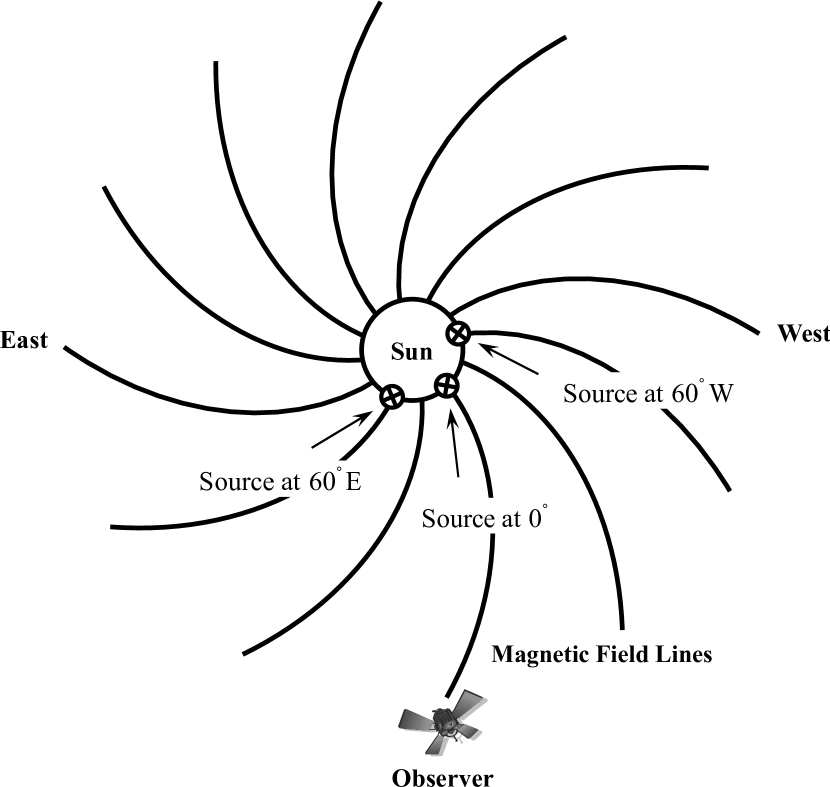
Figure 1: Diagram to illustrate the longitudinal locations of the particle sources in the solar equator relative to the magnetic footpoint of the observer, which is also located at $90^{\circ}$ colatitude. The center of the middle solar source is connected directly to the spacecraft by the interplanetary magnetic field line, whereas the centers of the solar sources on the left and right are $60^{\circ}$ east and $60^{\circ}$ west, respectively, away from the magnetic footpoint of the observer.

A diagram, i.e., Figure 1, serving as an example, is presented to illustrate the longitudinal locations of the particle sources on the solar surface relative to the magnetic footpoint of the observer, which is located at $90^{\circ}$ colatitude. In the scenario of the diagram, we can see that the center of the middle source on the Sun is connected directly to the spacecraft by interplanetary magnetic field line, whereas the centers of the solar sources on the left and right are $60^{\circ}$ east and $60^{\circ}$ west, respectively, away from the magnetic footpoint of the observer.

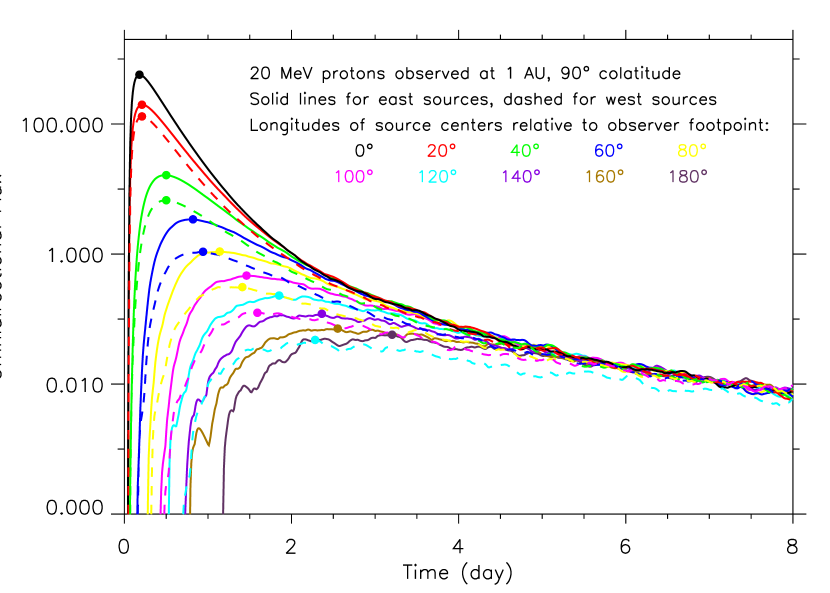
Figure 2: Flux-time profiles of the $20$ MeV SEPs originating from the different solar sources with different longitudinal locations relative to the magnetic footpoint of the observer at 1 AU, $90^{\circ}$ colatitude. With the same longitude separations between the magnetic field footpoint of the observer and solar sources, the SEP fluxes from solar sources located on the eastern side of the observer footpoint are larger than those from solar sources located on the western side. In addition, the SEP reservoir phenomenon is reproduced.

Figure 2 shows the flux-time profiles of the $20$ MeV SEPs originating from the different solar sources with different longitudinal locations relative to the magnetic footpoint of the observer at 1 AU, $90^{\circ}$ colatitude. In Figure 2, the solid and dashed lines denote the SEP omnidirectional fluxes originating from the east and west solar sources, respectively. The different colors of the curves represent different longitudinal distances between the magnetic footpoint of the observer and the solar sources. The $0^{\circ}$ relatively longitudinal distance denotes the case where the nominal magnetic footpoint of the observer and the solar source center locate at the same heliographic longitude. As we can see, the SEP flux in this case is the largest among all the cases investigated. This means that when the observer in the interplanetary space is nearly directly connected to the solar source by heliospheric magnetic field lines, the SEP flux is larger than that otherwise. However, a careful investigation based on our numerical simulations indicates that the maximum SEP flux shifts from the location of best magnetic connection and toward the east SEP sources with centers on relative longitudes $\sim-0.7^{\circ}-\sim-1.5^{\circ}$. We note that the shift extents depend on the ratio $\lambda_{\perp}/\lambda_{\parallel}$ of the perpendicular to the parallel mean free paths, the geometry of the magnetic spiral, the energy of SEPs, the coverage of the SEP sources, and the particle spatial distribution in the sources. In Figure 2, we can also see that the farther the magnetic field footpoint of the observer is away from the solar source, the smaller is the SEP flux observed and also the later the SEP event arrives at the observer’s position (see also He et al., 2011). Moreover, with the same longitude separations between the magnetic field footpoint of the observer and solar sources, the SEP fluxes from solar sources located on the eastern side of the observer footpoint are larger than those from solar sources located on the western side, and the times of onsets and maximum fluxes of SEP events from east sources are earlier than those from west sources. In other words, there exists an east-west longitudinally asymmetric distribution of SEPs in the heliosphere. In addition, we can obviously observe that in the decay phase the flux profiles of all the SEP cases have almost the same decay rate, which is called the SEP reservoir phenomenon in spacecraft observations. Therefore, our numerical simulations with a series of different SEP cases almost covering $360^{\circ}$ in heliographic longitude successfully reproduce the so-called SEP reservoir. The SEP reservoirs are observed by spacecraft at both low and high heliolatitudes, and by spacecraft at very different heliolongitudes and radial distances. In our simulations with perpendicular diffusion, we reproduce various SEP reservoirs (some results not shown here) at different heliospheric locations (longitude, latitude, and radial distance) without invoking the hypothesis of a reflecting boundary or diffusion barrier. Actually, it is difficult to imagine such an “overwhelming” reflecting boundary or diffusion barrier covering all the longitudes, all the latitudes, and even all the radial distances. Therefore, the perpendicular diffusion should be the dominant, if not the only, physical mechanism responsible for the formation of the SEP reservoirs.

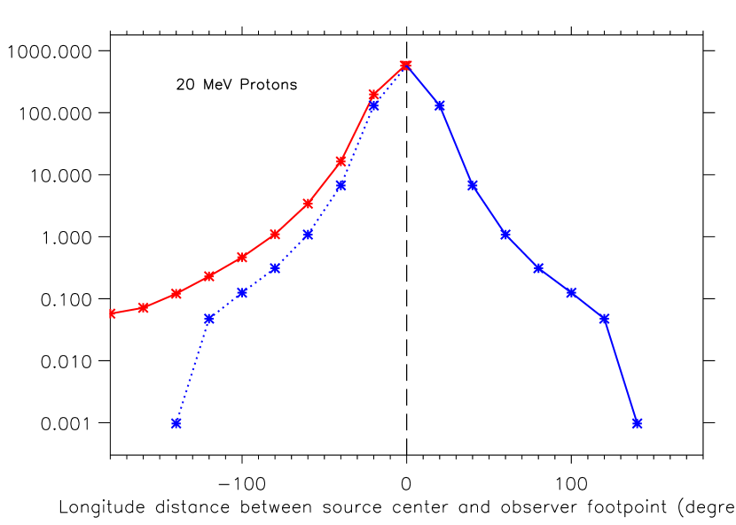
Figure 3: Flux maxima (peak fluxes) of the $20$ MeV SEPs originating from the different solar sources with different longitudinal locations relative to the magnetic footpoint of the observer at 1 AU, $90^{\circ}$ colatitude. With the same longitude separations between the solar source centers and the magnetic footpoint of the observer, the flux maxima of the SEP events originating from solar sources located on the eastern (left) side of the observer footpoint are systematically larger than those of the SEP events originating from sources located on the western (right) side.

The circles with different colors on the flux profiles in Figure 2 denote the peak fluxes of the corresponding SEP cases. We extract the information of the peak fluxes and the relevant longitudinal distances in the SEP cases investigated from Figure 2, and present it separately. In Figure 3, we show the peak fluxes of the $20$ MeV SEPs originating from the different solar sources with different longitudinal locations relative to the magnetic footpoint of the observer at 1 AU, $90^{\circ}$ colatitude. The X-axis in Figure 3 is the relatively longitudinal distance $\phi_{r}$ between the solar source center and the magnetic footpoint of the observer. The vertical dashed line in the middle of Figure 3 denotes the $0^{\circ}$ relatively longitudinal distance, where the nominal magnetic footpoint of the observer and the solar source center locate at the same heliographic longitude. As we can see, the peak flux in the SEP case with about $0^{\circ}$ relatively longitudinal distance is the largest among the cases investigated. This means that when the observer in the interplanetary space is nearly directly connected to the solar source by heliospheric magnetic field lines, the SEP peak flux is larger than that otherwise. However, a careful investigation indicates that the maximum SEP peak flux shifts from the place of best connection and toward the east SEP sources with centers on relative longitudes $\sim-0.7^{\circ}-\sim-1.5^{\circ}$. We connect the peak fluxes of SEPs in the simulated cases on the left-hand and right-hand halves with the red and blue curves, respectively. It can obviously be seen from Figure 3 that the farther the solar source center is away from the magnetic footpoint of the observer, the smaller is the peak flux of SEPs observed. We further mirror the peak fluxes of SEPs on the right-hand half to the left-hand half with a blue dotted curve. We can obviously observe that with the same longitude separations between the solar source centers and the magnetic footpoint of the observer, the peak fluxes of SEP events originating from solar sources located on the eastern side of the observer footpoint are systematically larger than those of the SEP events originating from sources located on the western side. Therefore, our relatively complete model calculation of SEP propagation with the effect of perpendicular diffusion shows that there exists an east-west asymmetry in the SEP intensities.

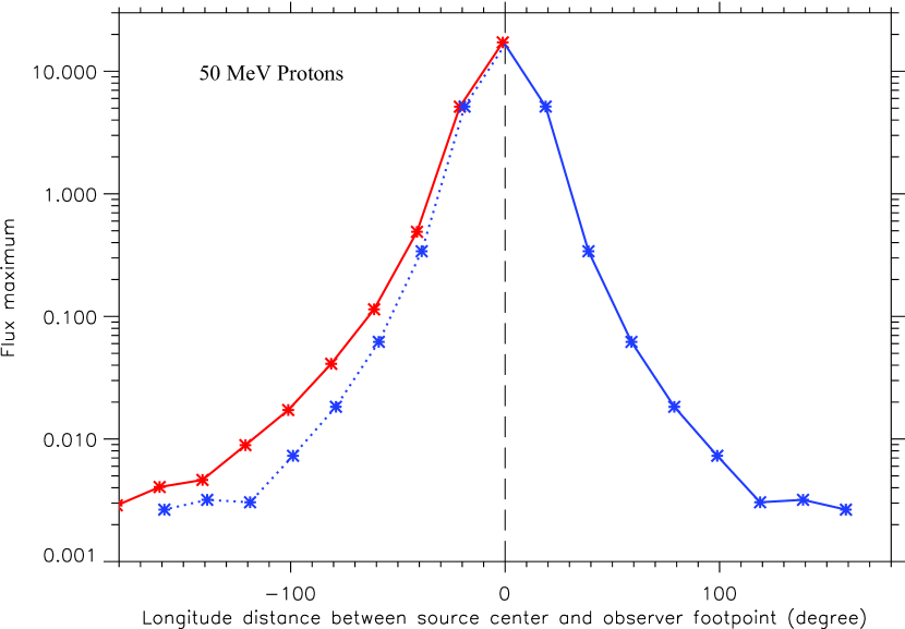
Figure 4: Flux maxima (peak fluxes) of the $50$ MeV SEPs originating from the different solar sources with different longitudinal locations relative to the magnetic footpoint of the observer at 1 AU, $90^{\circ}$ colatitude. With the same longitude separations between the solar source centers and the magnetic footpoint of the observer, the flux maxima of the SEP events originating from solar sources located on the eastern (left) side of the observer footpoint are systematically larger than those of the SEP events originating from sources located on the western (right) side.

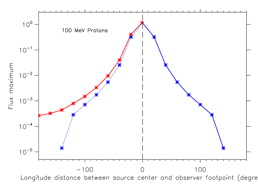
Figure 5: Flux maxima (peak fluxes) of the $100$ MeV SEPs originating from the different solar sources with different longitudinal locations relative to the magnetic footpoint of the observer at 1 AU, $90^{\circ}$ colatitude. With the same longitude separations between the solar source centers and the magnetic footpoint of the observer, the flux maxima of the SEP events originating from solar sources located on the eastern (left) side of the observer footpoint are systematically larger than those of the SEP events originating from sources located on the western (right) side.

Figure 4 shows the peak fluxes of the $50$ MeV SEPs originating from the different solar sources with different longitudinal distances relative to the magnetic footpoint of the observer at 1 AU, $90^{\circ}$ colatitude. As in Figure 3, we can also clearly observe that with the same longitudinal distances between the solar source centers and the magnetic footpoint of the observer, the peak fluxes of the SEP events originating from solar sources located on the eastern side of the observer footpoint are systematically larger than those of the SEP events originating from sources located on the western side. Therefore, the numerical simulation of the transport process of $50$ MeV SEPs also shows that there exists an east-west longitudinally asymmetric distribution of SEPs in the heliosphere. We note that the subtle difference between Figure 3 and Figure 4 results from the interplay of diffusion coefficients $\kappa_{\perp}$ and $\kappa_{\parallel}$ as well as the weak statistics of SEP fluxes in the cases with long longitudinal distances between the solar sources and the magnetic footpoint of the observer. Figure 5 shows the peak fluxes of the $100$ MeV SEPs originating from the different solar sources with different longitudinal distances relative to the magnetic footpoint of the observer at 1 AU, $90^{\circ}$ colatitude. It can also evidently be seen that with the same longitudinal distances between the solar source centers and the magnetic footpoint of the observer, the peak fluxes of the SEP events originating from solar sources located on the eastern side of the observer footpoint are systematically larger than those of the SEP events originating from sources located on the western side.

4 Implications of Simulation Results

Generally, an SEP event with a higher peak flux will reveal a larger intensity relative to other events through the entire evolution process (see Figure 2 and the results in He et al. (2011)). In general, the probability of the SEP events being observed by spacecraft near Earth’s orbit depends on the intensities of the particles in the events. An intense SEP event with high flux will experience relatively weak influences from interplanetary structures (such as magnetic cloud, heliospheric current sheet, corotating interaction region, etc.) during the propagation process in the heliosphere. However, the not so intense SEP events with small fluxes will be significantly affected by the interplanetary structures and then to weaken or even dissipate before entering Earth’s orbit. For example, numerous observations have shown that a magnetic cloud can considerably affect the propagation conditions of SEPs and low-energy cosmic rays, which is commonly observed as a decrease in the fluxes of the energetic particles (e.g., Blanco et al., 2013). Consequently, intense SEP events would have a larger probability of reaching Earth and being observed by spacecraft at 1 AU; whereas the relatively weak SEP events would have a lower probability to arrive at Earth and to be recorded by spacecraft.

As shown in the simulation results above, the SEP events originating from solar sources located on the eastern side of the magnetic footpoint of the observer reveal larger fluxes than those originating from solar sources located on the western side. Therefore, the SEP events originating from solar sources located at eastern relative longitudes would have a higher probability to reach Earth and to be observed by spacecraft near 1 AU. On the contrary, the SEP events from solar sources on the west side relative to the magnetic footpoint of observer will be more easily influenced by the interplanetary medium and structures, and then to weaken or even dissipate during their propagation processes. As a result, the spacecraft at 1 AU would have a larger probability to miss the SEP events originating from solar sources located at western relative longitudes.

5 Discussion

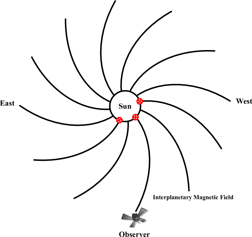
Figure 6: Sketch to show the east-west azimuthal asymmetry in the topology of the Parker interplanetary magnetic field. Due to the effects of the perpendicular diffusion and the azimuthally asymmetric geometry of the interplanetary magnetic field, with the same longitudinal distances between the solar sources and the magnetic footpoint of the observer, the SEPs originating from sources located on the eastern side of the observer footpoint are easier and more frequent than those from sources located on the western side to arrive at the observer in the interplanetary space.

Generally, as viewed from above the north pole of the Sun, the Parker spiral magnetic field lines originating from the solar surface would meander clockwise to somewhere in the interplanetary space with more eastern longitudes than their footpoints on the solar surface. This scenario can be seen in Figure 6. As we can see, there is an east-west azimuthal asymmetry in the topology of the Parker interplanetary magnetic field. According to the theoretical and observational investigations (e.g., Matthaeus et al., 2003; Bieber et al., 2004; He & Wan, 2012b), for physical conditions representative of the solar wind, the perpendicular diffusion coefficient would be a few percent of the parallel diffusion coefficient in magnitude. In general, SEPs would mainly transport along the average interplanetary magnetic field after they were produced from the surface of the Sun or a CME-driven shock. Therefore, when the observer is nearly directly connected to the solar source by the interplanetary magnetic field lines, the omnidirectional flux and peak flux of SEPs are larger than those in the cases where the observer is not connected directly to the solar sources. In general, the farther the solar source center is away from the magnetic footpoint of the observer, the smaller are the omnidirectional flux and peak flux of SEPs observed. In addition to the parallel diffusion, the SEPs will experience perpendicular diffusion to cross the heliospheric magnetic field lines during their transport processes in the interplanetary space. This is why the SEP events can be observed by a spacecraft that is not directly connected to the acceleration regions. In the limit of a point source release of SEPs and no perpendicular diffusion, the particles would also transport in longitude as a result of the field line rotating with the Sun. However, as Giacalone & Jokipii (2012) pointed out, in this case, the intensity profile of the event observed near 1 AU would be a spike of SEPs only seen when the field line containing the particles crosses the observer and would be zero for all other times, which is inconsistent with the usually observed shape of intensity profile of SEPs. A careful investigation based on our numerical simulations indicates that the maximum SEP flux shifts from the location of best magnetic connection and toward the east SEP sources with centers on relative longitudes $\sim-0.7^{\circ}-\sim-1.5^{\circ}$. Note that the shift extents depend on the ratio $\lambda_{\perp}/\lambda_{\parallel}$, the geometry of the magnetic spiral, the energy of SEPs, the coverage of the SEP sources, and the particle spatial distribution in the sources.

Due to the effects of the perpendicular diffusion and the azimuthally asymmetric geometry of the heliospheric magnetic field, with the same longitudinal distances between the solar sources and the magnetic footpoint of the observer, the SEPs originating from sources located on the eastern side of the observer footpoint are easier and more frequent than those from sources located on the western side to arrive at the observer in the interplanetary space. Consequently, with the same longitudinal distances between the solar sources and the observer footpoint, the fluxes of the SEP events associated with the solar sources located east are systematically larger than those of the SEP events associated with the sources located west. Accordingly, the peak intensities of the SEP events originating from solar sources located on the eastern side of the observer footpoint are also larger than those of the SEP events originating from sources located on the western side. Therefore, we propose that the longitudinally asymmetric distribution of SEPs results from the east-west azimuthal asymmetry in the topology of the Parker interplanetary magnetic field as well as the effects of perpendicular diffusion on the transport processes of SEPs in the heliosphere. Furthermore, the interplay between the perpendicular diffusion ($\lambda_{\perp}$) and the parallel diffusion ($\lambda_{\parallel}$) plays a very important role in determining the azimuthal asymmetry extents of the SEP distribution in the interplanetary space.

6 Summary and Conclusions

In the previous work of He et al. (2011), the authors reported and predicted that with the same longitude separation between the magnetic footpoint of observer and the solar sources, the SEPs produced and released from the sources located east are detected earlier with larger fluxes than those associated with the sources located west. This interesting phenomenon was called the “east-west azimuthal asymmetry of SEPs” by He et al. (2011). The figures in Giacalone & Jokipii (2012) using Parker’s equation also displayed east-west asymmetry in the SEP distribution. In this work, we systematically study the longitudinally asymmetric distribution of SEPs in view of numerical investigations. We carry out a series of relatively complete model calculations of SEP propagation with perpendicular diffusion in a three-dimensional interplanetary magnetic field. Our simulation results show that with the same longitude separation between the solar sources and the magnetic footpoint of the observer, the flux of SEPs released from the solar source located east is systematically higher than that of SEPs originating from the source located west. We conclude that the longitudinally asymmetric distribution of SEPs results from the east-west azimuthal asymmetry in the topology of the Parker interplanetary magnetic field as well as the effects of perpendicular diffusion on the transport processes of SEPs in the heliosphere. The interplay between the perpendicular diffusion ($\lambda_{\perp}$) and the parallel diffusion ($\lambda_{\parallel}$) plays an important role in determining the extents of the azimuthal asymmetry of the SEP distribution in the heliosphere.

In general, the probabilities of the SEP events being observed by spacecraft in the interplanetary space are proportional to the particle flux intensities in the events. Consequently, the SEP events originating from solar sources located at the eastern relative longitudes would be detected and recorded with somewhat higher probabilities by the observer near 1 AU. Therefore, the results presented in this work will be valuable for understanding the solar-terrestrial relations and useful in space weather forecasting.

References

- Beeck & Wibberenz (1986) Beeck, J., & Wibberenz, G. 1986, ApJ, 311, 437
- Beeck et al. (1987) Beeck, J., Mason, G. M., Hamilton, D. C., et al. 1987, ApJ, 322, 1052
- Bieber et al. (2004) Bieber, J. W., Matthaeus, W. H., Shalchi, A., & Qin, G. 2004, Geophys. Res. Lett., 31, L10805
- Blanco et al. (2013) Blanco, J. J., Hidalgo, M. A., Gómez-Herrero, R., et al. 2013, A&A, 556, A146
- Cane et al. (1988) Cane, H. V., Reames, D. V., & von Rosenvinge, T. T. 1988, J. Geophys. Res., 93, 9555
- Dresing et al. (2012) Dresing, N., Gómez-Herrero, R., Klassen, A., Heber, B., Kartavykh, Y., & Dröge, W. 2012, Sol. Phys., 281, 281
- Earl (1974) Earl, J. A. 1974, ApJ, 193, 231
- Giacalone & Jokipii (2012) Giacalone, J., & Jokipii, J. R. 2012, ApJ, 751, L33
- Hasselmann & Wibberenz (1968) Hasselmann, K., & Wibberenz, G. 1968, Z. Geophys., 34, 353
- Hasselmann & Wibberenz (1970) Hasselmann, K., & Wibberenz, G. 1970, ApJ, 162, 1049
- He & Qin (2011) He, H.-Q., & Qin, G. 2011, ApJ, 730, 46
- He et al. (2011) He, H.-Q., Qin, G., & Zhang, M. 2011, ApJ, 734, 74
- He & Wan (2012a) He, H.-Q., & Wan, W. 2012a, ApJ, 747, 38
- He & Wan (2012b) He, H.-Q., & Wan, W. 2012b, ApJS, 203, 19
- He & Wan (2013a) He, H.-Q., & Wan, W. 2013a, in Proceedings of the 33rd International Cosmic Ray Conference, ID 0267, Rio de Janeiro (Brazil), July 2-9, 2013
- He & Wan (2013b) He, H.-Q., & Wan, W. 2013b, A&A, 557, A57
- He & Schlickeiser (2014) He, H.-Q., & Schlickeiser, R. 2014, ApJ, 792, 85
- Hundhausen (1993) Hundhausen, A. J. 1993, J. Geophys. Res., 98, 13177
- Isenberg (1997) Isenberg, P. A. 1997, J. Geophys. Res., 102, 4719
- Jokipii (1966) Jokipii, J. R. 1966, ApJ, 146, 480
- Kóta & Jokipii (1997) Kóta, J., & Jokipii, J. R. 1997, in Proc. 25th ICRC, 1, 213
- Li et al. (2003) Li, G., Zank, G. P., & Rice, W. K. M. 2003, J. Geophys. Res., 108, 1082
- Maia et al. (2001) Maia, D., Pick, M., Hawkins III, S. E., Fomichev, V. V., & , K. 2001, Sol. Phys., 204, 199
- Matthaeus et al. (2003) Matthaeus, W. H., Qin, G., Bieber, J. W., & Zank, G. P. 2003, ApJ, 590, L53
- Ng & Gleeson (1971) Ng, C. K., & Gleeson, L. J. 1971, Sol. Phys., 20, 166
- Ng & Wong (1979) Ng, C. K., & Wong, K. Y. 1979, in Proc. 16th ICRC, 5, 252
- Parker (1965) Parker, E. N. 1965, Planet. Space Sci., 13, 9
- Qin et al. (2011) Qin, G., He, H.-Q., & Zhang, M. 2011, ApJ, 738, 28
- Reames (1999) Reames, D. V. 1999, Space Sci. Rev., 90, 413
- Reid (1964) Reid, G. C. 1964, J. Geophys. Res., 69, 2659
- Roelof (1969) Roelof, E. C. 1969, in Lectures in High Energy Astrophysics, ed. H. Ogelmann & J. R. Wayland (NASA SP-199; Washington, DC: NASA), 111
- Ruffolo (1991) Ruffolo, D. 1991, ApJ, 382, 688
- Schlickeiser (2002) Schlickeiser, R. 2002, Cosmic Ray Astrophysics (Berlin: Springer)
- Shalchi et al. (2004) Shalchi, A., Bieber, J. W., & Matthaeus, W. H. 2004, ApJ, 604, 675
- Skilling (1971) Skilling, J. 1971, ApJ, 170, 265
- Wang et al. (2006) Wang, Y.-M., Pick, M., & Mason, G. M. 2006, ApJ, 639, 495
- Zank et al. (2000) Zank, G. P., Rice, W. K. M., & Wu, C. C. 2000, J. Geophys. Res., 105, 25079
- Zhang (1999) Zhang, M. 1999, ApJ, 513, 409
- Zhang et al. (2009) Zhang, M., Qin, G., & Rassoul, H. 2009, ApJ, 692, 109